45
Mobile Communications Systems Problems Luis M. Correia February 2015

Mobile
Communications
Systems
Problems
Luis M. Correia
February 2015
2
STATISTICAL DISTRIBUTIONS IN TELECOMMUNICATIONS
Questions
1. Prove that, for any statistical distribution, one has:
222 xxx
2. Calculate the parameters of the Uniform Distribution.
3. Consider a random variable with Normal Distribution, zero mean, and mean square value
of 9. Calculate α, such that |x| < α, with a probability of: i) 90 %; ii) 99 %; iii) 99.99 %.
4. Find the PDF of the Log-Normal Distribution, taking the Normal Distribution as a starting
point, taking the transformation of random variables:
pz(z) = px[x(z)] |dx/dz|
5. Verify that, when x ~ x0, the PDF of the Rice Distribution can be approximated by:
a) Rayleigh Distribution, for 22
0 Rxx ;
b) Normal Distribution, for 22
0 Rxx .
Suggestion: consider the following approximations for the modified Bessel function:
1,π2
e
1,eI
2
0u
u
uu u
u
6. Consider an electric field magnitude described by the Rayleigh Distribution. Find the PDF
of the new distribution when the electric field magnitude is expressed in dBµV/m.
7. Find the PDF of the power density, when the electric field magnitude is described by the
Rayleigh Distribution.
8. Calculate the probability of signal magnitude, described by the Rayleigh Distribution, to be
within an interval of ±3 dB relative to its root mean square value.

3
9. Estimate the probability of a signal magnitude, described by the Rice Distribution, to be
within an interval of ±3 dB relative to the magnitude of the direct component, when:
i) KR = 0 dB; ii) KR = 7.5 dB; iii) KR = 13 dB.
10. The CDF of the 50-90 % deviation of the path loss measured in a certain area is shown in
the figure below, using a Normal scale. The straight line represents the best fit for the
measures in the interval [5, 95] %. Calculate, in dB, from the figure, the path loss average,
standard deviation, and mean square values.

4
STATISTICAL DISTRIBUTIONS IN TELECOMMUNICATIONS
Solutions
3.
Prob [%] 90 99 99.99
α 4.937 7.731 11.673
6.
22 2
2exp2exp
1
EE m
L
LmLp
EEE , E = E[dBµV/m] , L = 20/ln(10)
7. SS
SSp e
1
8. 47.12 %
9.
KR [dB] 0 7.5 13
Prob [%] 50. 78. 95.5
10. dB24.4 L , dB36.1L , dB83.192 L
5
PROPAGATION MODELS
Questions
1. Establish the expressions given below, from the corresponding ones in linear units.
a) Pr [dBW] = -32.44 + Pt [dBW] + Gt [dBi] + Gr [dBi] - 20 log(d[km]) - 20 log(f[MHz])
b) Er [dBµV/m] = 74.77 + Pt [dBW] + Gt [dBi] - 20 log(d[km])
c) Pr [dBm] = -77.21 + Er [dBµV/m] + Gr [dBi] - 20 log(f[MHz])
2. Establish the expression for the path loss, in dB, as a function of the electric field
magnitude, when the BS has a half wavelength dipole fed by 1 kW.
3. Show that, in the Flat Earth approximation, although the electric field magnitude is
proportional to frequency, the open-circuit voltage at a receiving half wavelength dipole is
independent of frequency.
4. Calculate the minimum distance for which the approximate expression for the electric field
magnitude on Flat Earth is valid, under f = 450, 900, 1800 MHz, hr = 1.8, 3.0 m, and
ht = 50, 100, 200 m. Comment on the application of this expression for the calculation of
coverage by a BS on a 10 km radius.
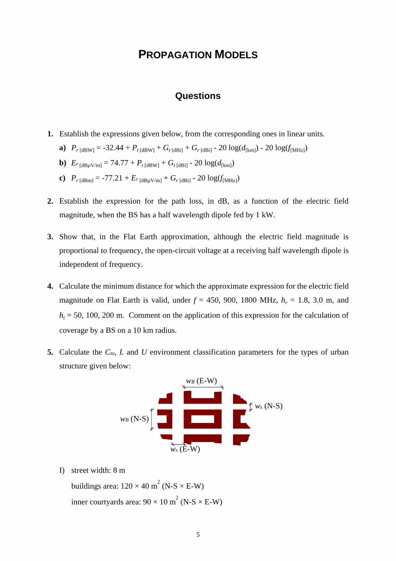
5. Calculate the Cto, L and U environment classification parameters for the types of urban
structure given below:
I) street width: 8 m
buildings area: 120 × 40 m2 (N-S × E-W)
inner courtyards area: 90 × 10 m2 (N-S × E-W)
ws (E-W)
ws (N-S)
wB (N-S)
wB (E-W)
6
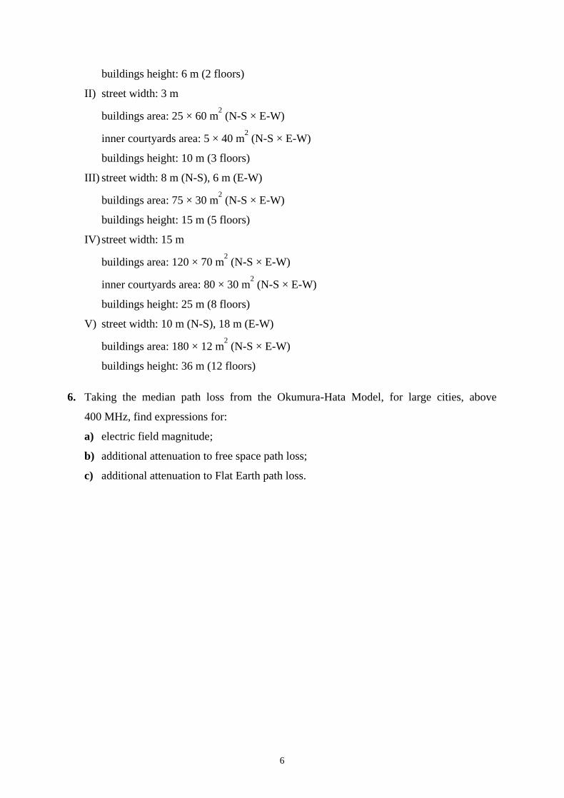
buildings height: 6 m (2 floors)
II) street width: 3 m
buildings area: 25 × 60 m2 (N-S × E-W)
inner courtyards area: 5 × 40 m2 (N-S × E-W)
buildings height: 10 m (3 floors)
III) street width: 8 m (N-S), 6 m (E-W)
buildings area: 75 × 30 m2 (N-S × E-W)
buildings height: 15 m (5 floors)
IV) street width: 15 m
buildings area: 120 × 70 m2 (N-S × E-W)
inner courtyards area: 80 × 30 m2 (N-S × E-W)
buildings height: 25 m (8 floors)
V) street width: 10 m (N-S), 18 m (E-W)
buildings area: 180 × 12 m2 (N-S × E-W)
buildings height: 36 m (12 floors)
6. Taking the median path loss from the Okumura-Hata Model, for large cities, above
400 MHz, find expressions for:
a) electric field magnitude;
b) additional attenuation to free space path loss;
c) additional attenuation to Flat Earth path loss.
7
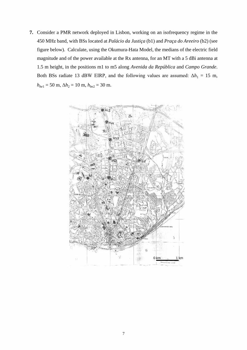
7. Consider a PMR network deployed in Lisbon, working on an isofrequency regime in the
450 MHz band, with BSs located at Palácio da Justiça (b1) and Praça do Areeiro (b2) (see
figure below). Calculate, using the Okumura-Hata Model, the medians of the electric field
magnitude and of the power available at the Rx antenna, for an MT with a 5 dBi antenna at
1.5 m height, in the positions m1 to m5 along Avenida da República and Campo Grande.
Both BSs radiate 13 dBW EIRP, and the following values are assumed: Δh1 = 15 m,
hbe1 = 50 m, Δh2 = 10 m, hbe2 = 30 m.
0 km 1 km
8
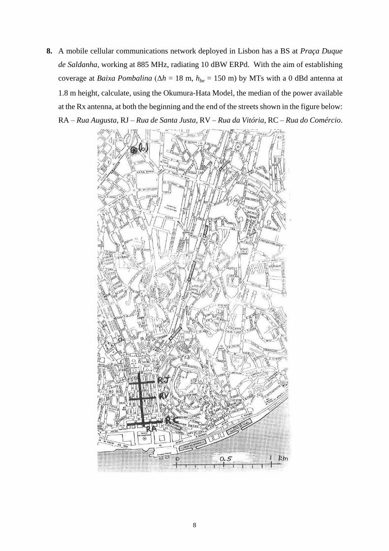
8. A mobile cellular communications network deployed in Lisbon has a BS at Praça Duque
de Saldanha, working at 885 MHz, radiating 10 dBW ERPd. With the aim of establishing
coverage at Baixa Pombalina (Δh = 18 m, hbe = 150 m) by MTs with a 0 dBd antenna at
1.8 m height, calculate, using the Okumura-Hata Model, the median of the power available
at the Rx antenna, at both the beginning and the end of the streets shown in the figure below:
RA – Rua Augusta, RJ – Rua de Santa Justa, RV – Rua da Vitória, RC – Rua do Comércio.

9
9. Consider a PMR network, with a BS on the top of Parque de Monsanto (designated by (b)
in the figure below), radiating 14 dBW EIRP at 421 MHz. Use the Okumura-Hata Model,
in order to calculate the median of the power available at the Rx antenna, for MTs with a
7 dBi antenna at 2.5 m height, in the areas of Almada, Barreiro, Montijo and Alcochete,
where one can take hbe = 250 m, and neglect Δh.
10. Calculate the coverage ranges for the below specified system, for 50, 90 and 99 % of the
locations, using the Okumura-Hata Model in urban, suburban, and rural environments:
f = 900 MHz
Pb = 25 W, Gb = 5 dBi, hbe = 50 m
Pm min = -100 dBm, Gm = 2 dBi, hm = 1.8 m
11. A GSM BS is located at Boca do Inferno (Cascais), radiating 16 dBW ERPd at 900 MHz,
the antenna being 50 m above see level. Calculate the maximum distance within which an
MT in a yacht can communicate, with a 0 dBd antenna 2 m above see level, assuming an
Rx sensitivity of -85 dBm. Use both the Flat Earth and the Okumura-Hata Models, and
comment on the results.

10
12. The BS of a PMR network, working at 450 MHz, has the following characteristics:
Pb = 10 dBW; Gb = 2 dBi; hb = 30 m. Calculate, using the Okumura-Hata Model, the
electric field magnitude and the power available at the Rx antenna, for an MT with a 2 dBi
antenna at 1.5 m height, at a distance of 20 km in an urban environment, for 1, 10, 50, 90,
and 99 % of the locations.
13. A mobile cellular communications network, working at 850 MHz, has the antenna of a BS,
with a 5 dBd gain fed with 17 dBW, at a height of 40 m above the average terrain level.
Using the Okumura-Hata Model, calculate the percentage of locations covered at 35 km
away from the BS, in a rural environment, by MTs with a 0 dBd antenna at 1.8 m height,
and an Rx sensitivity of -90 dBm. Recalculate the value for MTs with 5 dBd antennas, and
compare the results.
14. Find, for the Ikegami Model, considering the MT at the street centre, taking |Γ| = -6 dB,
expressions for:
a) path loss;
b) additional attenuation to free space path loss.
15. Calculate, for the Ikegami Model, taking |Γ| = -6 dB, the difference in electric field
magnitude (in dB) between the axes of the two lanes of a street (take ws/4 and 3ws/4,
ws being the street width). Comment on the results.
16. Using the Ikegami Model, calculate the path loss at the centre of the streets associated to
the various types of urban structure shown in Question 5, when the network operates at
900 MHz. Consider that: waves propagate perpendicular to streets’ axes; MTs’ are 5 km
away from the BS, with antennas 1.8 m above ground; the BS antenna is slightly higher
than roof tops; building walls reflect -6 dB.
17. Find an expression for the additional attenuation to free space path loss, for the Walfisch-
Bertoni Model, with the explicit dependence on frequency (in MHz) and distance (in km),
under the following conditions: building heights are much larger that MTs’; MTs are at the
street centre; street widths are equal to building heights.

11
18. Calculate, for the Walfisch-Bertoni Model, taking street widths equal to building heights,
and considering that building heights are much larger that MTs’, the difference in electric
field magnitude (in dB) between the axes of the two lanes of a street (take ws/4 and 3ws/4,
ws being the street width). Comment on the results.
19. Using the Walfisch-Bertoni Model, calculate the path loss at the centre of the streets
associated to the various types of urban structure shown in Question 5, when the network
operates at 900 MHz. Consider that: waves propagate perpendicular to streets’ axes; MTs’
are 5 km away from the BS, with antennas 1.8 m above ground; the BS antenna is 50 m
above ground. Compare the results with those obtained from the Ikegami Model (Question
16).
20. Using the COST231-Walfisch-Ikegami Model, calculate the path loss at the centre of the
streets associated to the various types of urban structure shown in Question 5, when the
network operates at 900 MHz. Consider that: waves propagate perpendicular to streets’
axes; MTs’ are 5 km away from the BS, with antennas 1.8 m above ground; the BS antenna
is 50 m above ground; type I is an urban area, while all others are dense urban ones.
Compare the results with those obtained from the Ikegami and Walfisch-Bertoni Models
(Questions 16 and 19).
21. Consider the following system:
f = 900 MHz
PbGb = 20 dBW, hbe = 150 m
Pm min = -100 dBm, Gm = 2 dBi, hm = 1.8 m
Using the Okumura-Hata Model in urban environments (small cities over flat terrain),
calculate the percentage of:
a) locations served 20 km away from the BS;
b) locations served 20 km away from the BS, but when Pm min = -80 dBm;
c) locations served within a radius of 20 km away from the BS.
12
PROPAGATION MODELS
Solutions
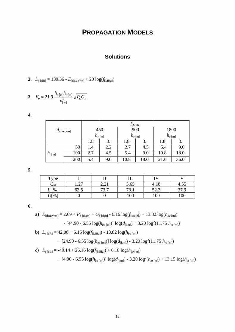
2. Lp [dB] = 139.36 - E[dBµV/m] + 20 log(f[MHz])
3.
EE
REGP
d
hhV
2
m
mm
0 9.21
4.
f[MHz]
dmin [km] 450
hr [m]
900
hr [m]
1800
hr [m]
1.8 3. 1.8 3. 1.8 3.
50 1.4 2.2 2.7 4.5 5.4 9.0
ht [m] 100 2.7 4.5 5.4 9.0 10.8 18.0
200 5.4 9.0 10.8 18.0 21.6 36.0
5.
Type I II III IV V
Cto 1.27 2.21 3.65 4.18 4.55
L [%] 63.5 73.7 73.1 52.3 37.9
U[%] 0 0 100 100 100
6.
a) E[dBµV/m] = 2.69 + Pb [dBm] + Gb [dBi] - 6.16 log(f[MHz]) + 13.82 log(hbe [m])
- [44.90 - 6.55 log(hbe [m])] log(d[km]) + 3.20 log2(11.75 hm [m])
b) Ls [dB] = 42.08 + 6.16 log(f[MHz]) - 13.82 log(hbe [m])
+ [24.90 - 6.55 log(hbe [m])] log(d[km]) - 3.20 log2(11.75 hm [m])
c) Ls [dB] = -49.14 + 26.16 log(f[MHz]) + 6.18 log(hbe [m])
+ [4.90 - 6.55 log(hbe [m])] log(d[km]) - 3.20 log2(hm [m]) + 13.15 log(hm [m])

13
7.
Location m1 m2 m3 m4 m5
E[dBµV/m] b1 57.79 53.94 48.38 44.35 41.68
b2 48.52 50.71 47.53 42.66 39.53
Pm [dBm] b1 -67.48 -71.33 -76.89 -80.92 -83.59
b2 -76.75 -74.56 -77.74 -82.61 -85.74
8.
Location beginning end
RA -75.7 -78.4
RJ -89.3
Pm [dBm] RV -89.7
RC -90.7
9.
Location Almada Barreiro Montijo Alcochete
Pm [dBm] -48.4 -55.4 -66.2 -60.6
10.
d[km] Environment
urban suburban rural
50 6.9 13.5 48.0*
Prob. [%] 90 2.9 5.5 19.4
99 1.4 2.6 9.3
* - out of range.
11.
OHM
FEMd
,1.38
,1.24kmmax
12.
Prob. [%] 1 10 50 90 99
Pm [dBm] -98.5 -108.3 -120.4 -132.4 -142.2
Em [dBµV/m] 29.8 19.9 7.9 -4.1 -13.9
13. 42.3 % @ 0 dBd, 61.5 % @ 5 dBd
14.
a) Lp [dB] = 24.25 + 30 log(f[MHz]) + 20 log(d[km]) - 10 log(ws[m]) + 20 log(HB [m] - hm [m])
+ 10 log[sin(φ)]
b) Ls [dB] = -8.19 + 10 log(f[MHz]) - 10 log(ws[m]) + 20 log(HB [m] - hm [m]) + 10 log[sin(φ)]
14
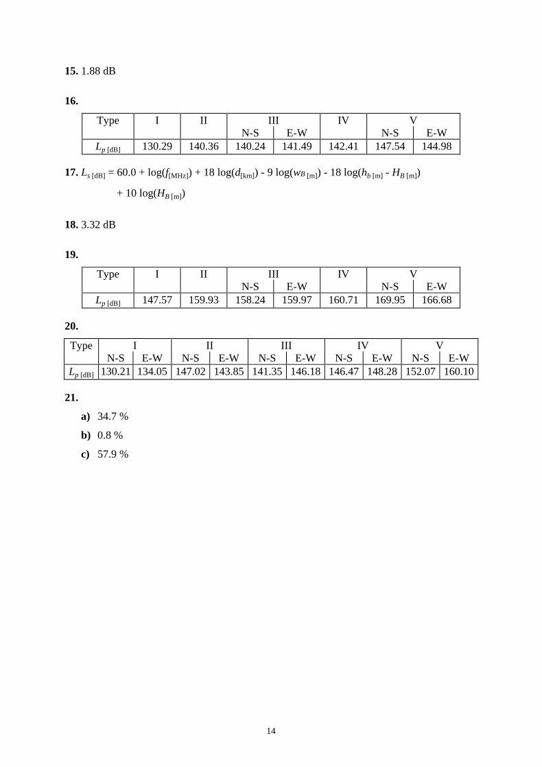
15. 1.88 dB
16.
Type I II III IV V
N-S E-W N-S E-W
Lp [dB] 130.29 140.36 140.24 141.49 142.41 147.54 144.98
17. Ls [dB] = 60.0 + log(f[MHz]) + 18 log(d[km]) - 9 log(wB [m]) - 18 log(hb [m] - HB [m])
+ 10 log(HB [m])
18. 3.32 dB
19.
Type I II III IV V
N-S E-W N-S E-W
Lp [dB] 147.57 159.93 158.24 159.97 160.71 169.95 166.68
20.
Type I II III IV V
N-S E-W N-S E-W N-S E-W N-S E-W N-S E-W
Lp [dB] 130.21 134.05 147.02 143.85 141.35 146.18 146.47 148.28 152.07 160.10
21.
a) 34.7 %
b) 0.8 %
c) 57.9 %
15
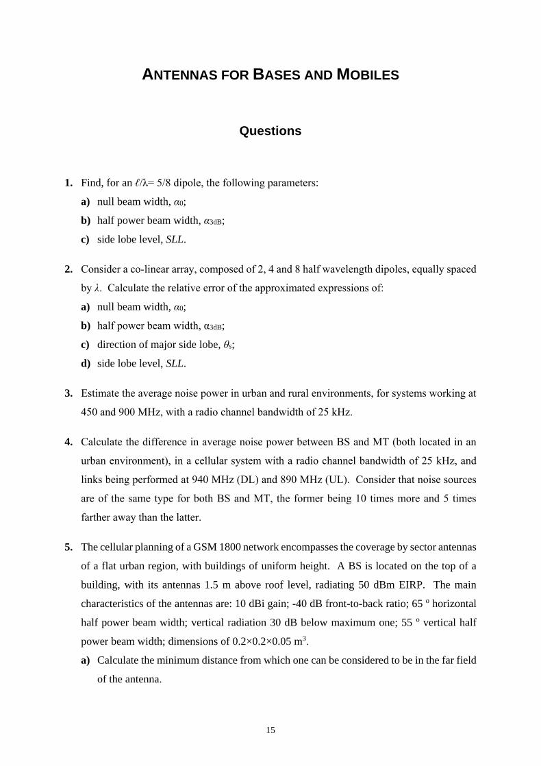
ANTENNAS FOR BASES AND MOBILES
Questions
1. Find, for an ℓ/λ= 5/8 dipole, the following parameters:
a) null beam width, α0;
b) half power beam width, α3dB;
c) side lobe level, SLL.
2. Consider a co-linear array, composed of 2, 4 and 8 half wavelength dipoles, equally spaced
by λ. Calculate the relative error of the approximated expressions of:
a) null beam width, α0;
b) half power beam width, α3dB;
c) direction of major side lobe, θs;
d) side lobe level, SLL.
3. Estimate the average noise power in urban and rural environments, for systems working at
450 and 900 MHz, with a radio channel bandwidth of 25 kHz.
4. Calculate the difference in average noise power between BS and MT (both located in an
urban environment), in a cellular system with a radio channel bandwidth of 25 kHz, and
links being performed at 940 MHz (DL) and 890 MHz (UL). Consider that noise sources
are of the same type for both BS and MT, the former being 10 times more and 5 times
farther away than the latter.
5. The cellular planning of a GSM 1800 network encompasses the coverage by sector antennas
of a flat urban region, with buildings of uniform height. A BS is located on the top of a
building, with its antennas 1.5 m above roof level, radiating 50 dBm EIRP. The main
characteristics of the antennas are: 10 dBi gain; -40 dB front-to-back ratio; 65 o horizontal
half power beam width; vertical radiation 30 dB below maximum one; 55 o vertical half
power beam width; dimensions of 0.2×0.2×0.05 m3.
a) Calculate the minimum distance from which one can be considered to be in the far field
of the antenna.
16
b) Estimate the power density of the electromagnetic radiation to which people are
exposed, under the most unfavourable conditions, in the floor just below the antennas.
c) Estimate the power density of the electromagnetic radiation to which people are
exposed, under the most unfavourable conditions, 10 m away on a balcony of the
building located on the other side of the street.
d) Estimate the distance where the exposure reference level is verified, on the two ways of
the direction of maximum radiation of the antenna.
17
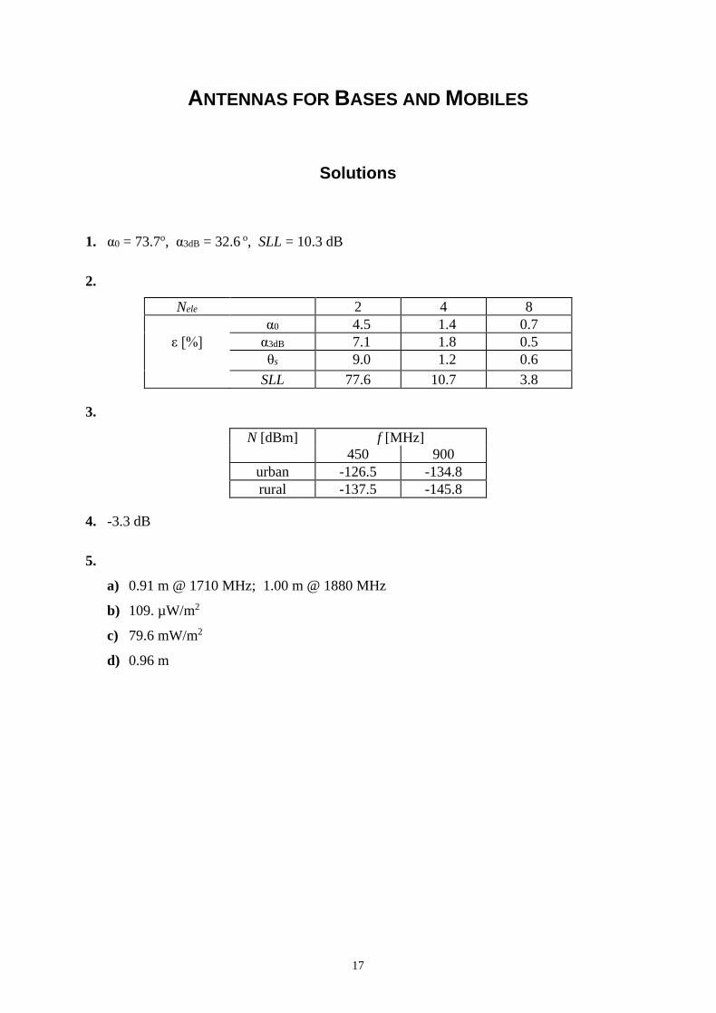
ANTENNAS FOR BASES AND MOBILES
Solutions
1. α0 = 73.7o, α3dB = 32.6 o, SLL = 10.3 dB
2.
Nele 2 4 8
α0 4.5 1.4 0.7
ε [%] α3dB 7.1 1.8 0.5
θs 9.0 1.2 0.6
SLL 77.6 10.7 3.8
3.
N [dBm] f [MHz]
450 900
urban -126.5 -134.8
rural -137.5 -145.8
4. -3.3 dB
5.
a) 0.91 m @ 1710 MHz; 1.00 m @ 1880 MHz
b) 109. µW/m2
c) 79.6 mW/m2
d) 0.96 m
18
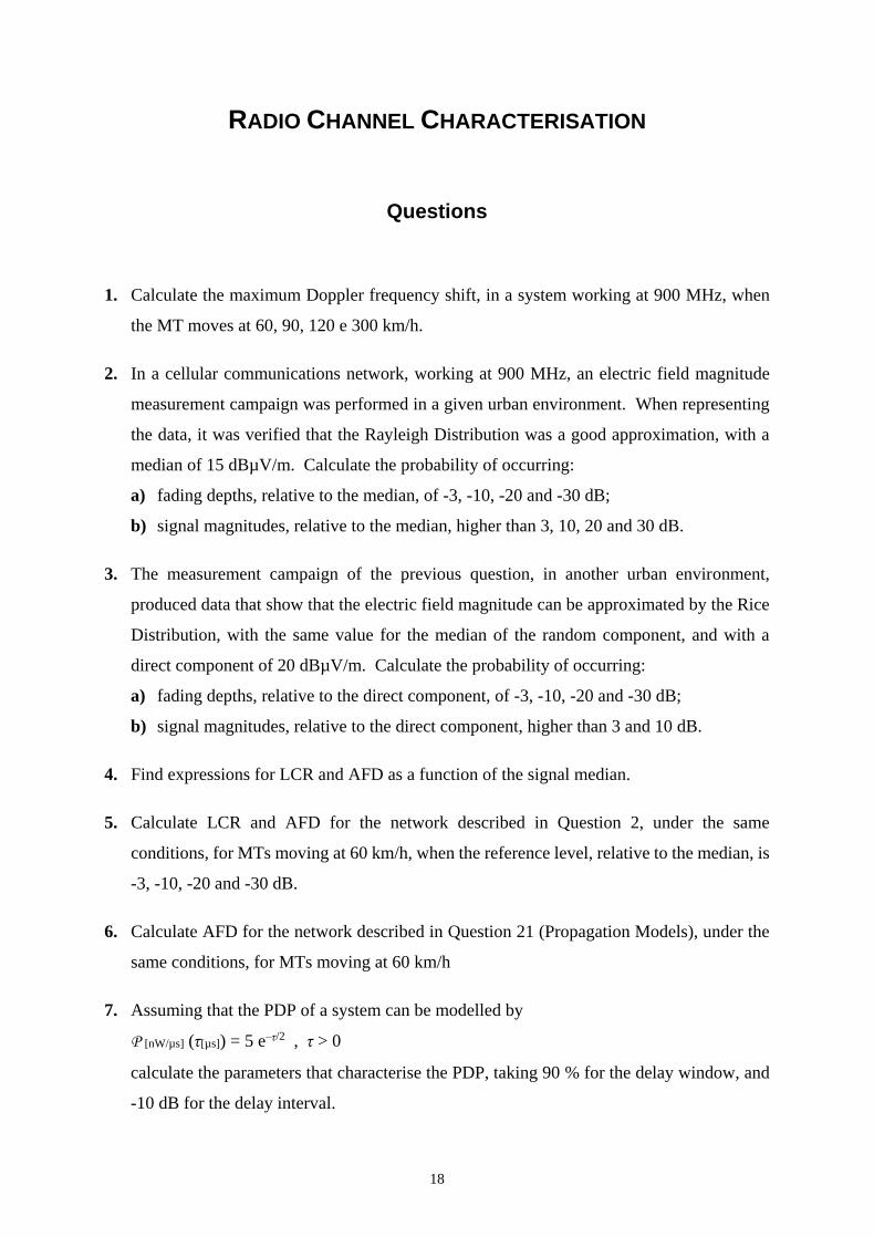
RADIO CHANNEL CHARACTERISATION
Questions
1. Calculate the maximum Doppler frequency shift, in a system working at 900 MHz, when
the MT moves at 60, 90, 120 e 300 km/h.
2. In a cellular communications network, working at 900 MHz, an electric field magnitude
measurement campaign was performed in a given urban environment. When representing
the data, it was verified that the Rayleigh Distribution was a good approximation, with a
median of 15 dBµV/m. Calculate the probability of occurring:
a) fading depths, relative to the median, of -3, -10, -20 and -30 dB;
b) signal magnitudes, relative to the median, higher than 3, 10, 20 and 30 dB.
3. The measurement campaign of the previous question, in another urban environment,
produced data that show that the electric field magnitude can be approximated by the Rice
Distribution, with the same value for the median of the random component, and with a
direct component of 20 dBµV/m. Calculate the probability of occurring:
a) fading depths, relative to the direct component, of -3, -10, -20 and -30 dB;
b) signal magnitudes, relative to the direct component, higher than 3 and 10 dB.
4. Find expressions for LCR and AFD as a function of the signal median.
5. Calculate LCR and AFD for the network described in Question 2, under the same
conditions, for MTs moving at 60 km/h, when the reference level, relative to the median, is
-3, -10, -20 and -30 dB.
6. Calculate AFD for the network described in Question 21 (Propagation Models), under the
same conditions, for MTs moving at 60 km/h
7. Assuming that the PDP of a system can be modelled by
P [nW/µs] (τ[µs]) = 5 e–τ/2 , τ > 0
calculate the parameters that characterise the PDP, taking 90 % for the delay window, and
-10 dB for the delay interval.

19
8. Find an expression for the coherence bandwidth, when the correlation coefficient is 0.9,
and compare it with the one obtained for 0.5.
9. Consider a GSM 900 BS installed in an urban environment, where MTs move at 4 km/h,
receiving multipath waves on a horizontal plane, angularly described by a Uniform
Distribution in 2, and experiencing a delay spread of 3 µs. Analyse the possibility of using
order 2 diversity at the BS, in space, time, and frequency, in the entire bandwidth.
N.B.: J0(z0 n) = 0, z0 n = 2.405, 5.520, 8.654, 11.792, ...
10. A GSM 900 BS, installed in an urban environment, has two receiving antennas horizontally
spaced by 2 m, with their axis perpendicular to the axis of a street, which has a width of
10 m. Analyse the variation of the correlation coefficient, and of the corresponding
diversity gain, when MTs are between 50 and 500 m away from the BS.
11. Compare the outage probability and the SNR average value at the output of the combiner,
between PSC, TSC ( 0 T ) and EGC compared to MRC, for an order 2 diversity scheme,
when the SNR decision level is much lower than the mean value obtained without diversity.
N.B.: (M-1/2)! = (2M-1)!/2M
12. Calculate the outage probability of an order 2 PSC combiner, when the SNR decision level
equals a fourth of the mean value obtained without diversity, and compare it with the one
obtained without diversity.
13. Calculate the minimum order of an MRC combiner, leading to an outage probability, at
least, two orders of magnitude lower than the one obtained without diversity, for an SNR
decision level 10 dB below the mean value obtained without diversity.
14. Consider a noiseless channel, with an impulsive response given by
hc(t) = a0 δ(t-t0) + a1 δ(t-t1)
where a1 << a0 and t1 > t0. Calculate the coefficients of a corresponding order 3 equaliser,
and analyse the resulting error.
15. Find the equations that rule equalisers coefficients, as a function of the characteristics a
noiseless channel, in the ZF case.
20
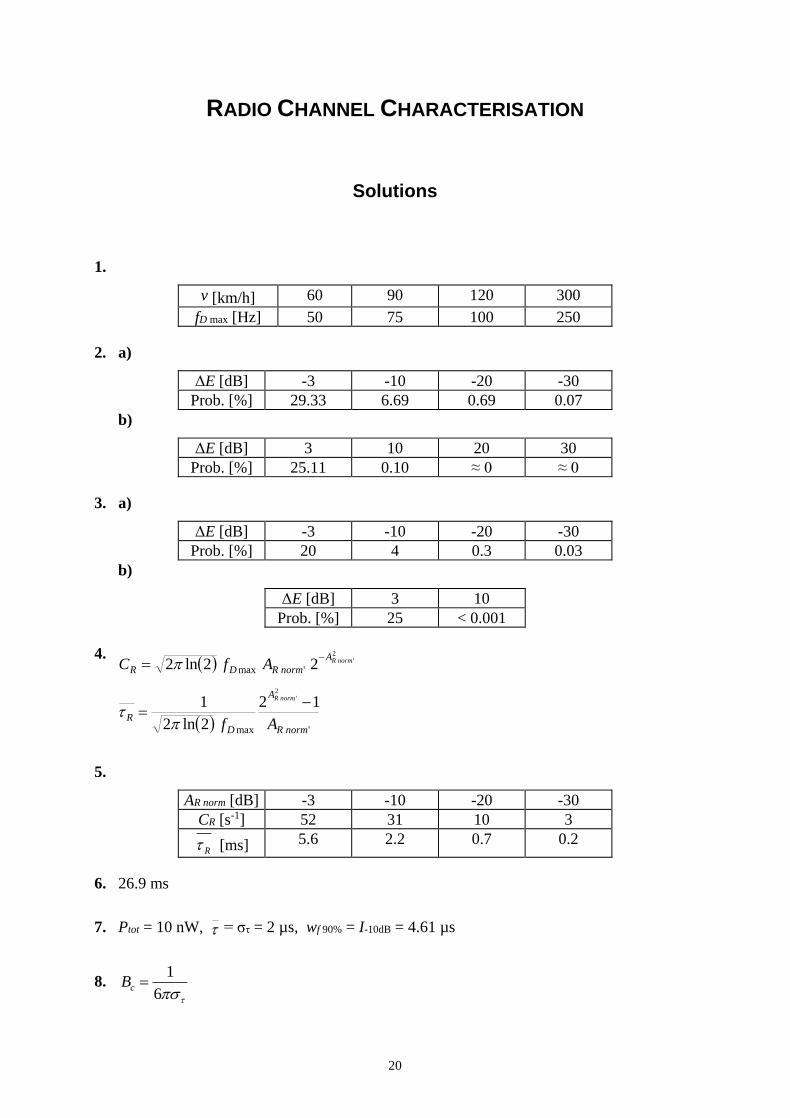
RADIO CHANNEL CHARACTERISATION
Solutions
1.
v [km/h] 60 90 120 300
fD max [Hz] 50 75 100 250
2. a)
ΔE [dB] -3 -10 -20 -30
Prob. [%] 29.33 6.69 0.69 0.07
b)
ΔE [dB] 3 10 20 30
Prob. [%] 25.11 0.10 ≈ 0 ≈ 0
3. a)
ΔE [dB] -3 -10 -20 -30
Prob. [%] 20 4 0.3 0.03
b)
ΔE [dB] 3 10
Prob. [%] 25 < 0.001
4.
2'22ln2 'max
normRA
normRDR AfC
'max
12
2ln2
12
'
normR
A
D
RAf
normR
5.
AR norm [dB] -3 -10 -20 -30
CR [s-1] 52 31 10 3
R [ms] 5.6 2.2 0.7 0.2
6. 26.9 ms
7. Ptot = 10 nW, = στ = 2 µs, wf 90% = I-10dB = 4.61 µs
8. 6
1cB
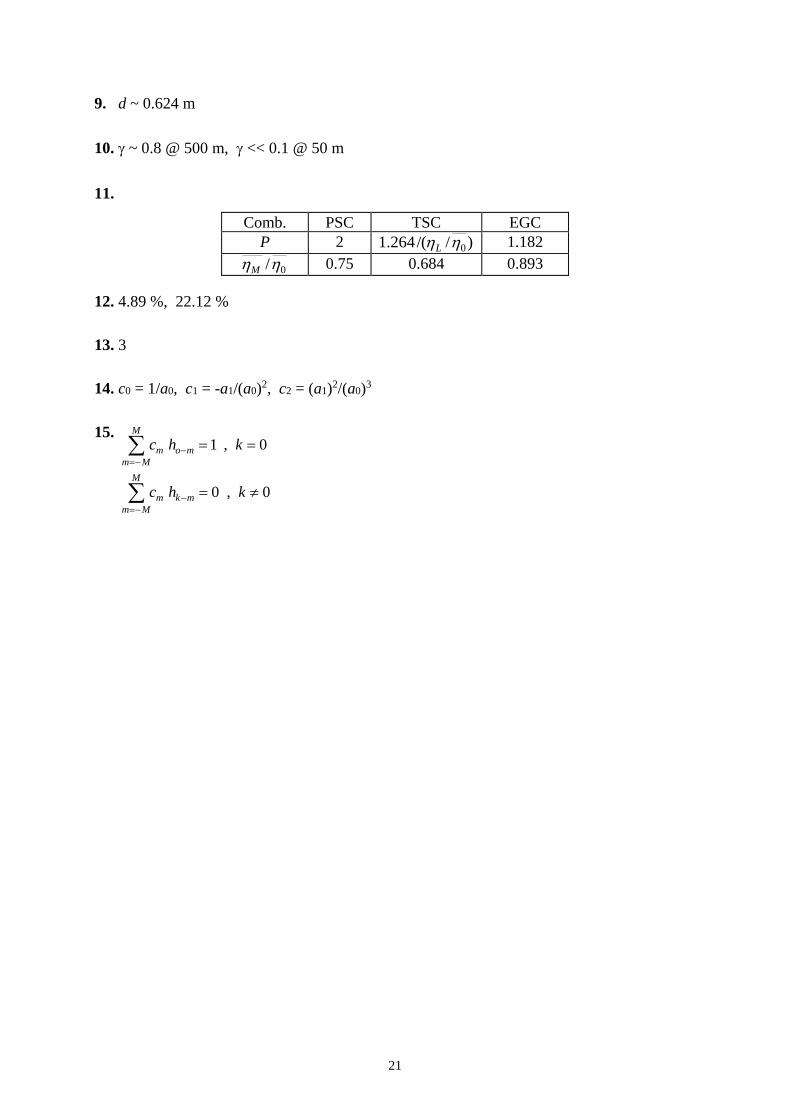
21
9. d ~ 0.624 m
10. ~ 0.8 @ 500 m, << 0.1 @ 50 m
11.
Comb. PSC TSC EGC
P 2 )//(264.1 0L
1.182
0/M
0.75 0.684 0.893
12. 4.89 %, 22.12 %
13. 3
14. c0 = 1/a0, c1 = -a1/(a0)2, c2 = (a1)2/(a0)3
15.
0,0
0,1
khc
khc
M
Mm
mkm
M
Mm
mom
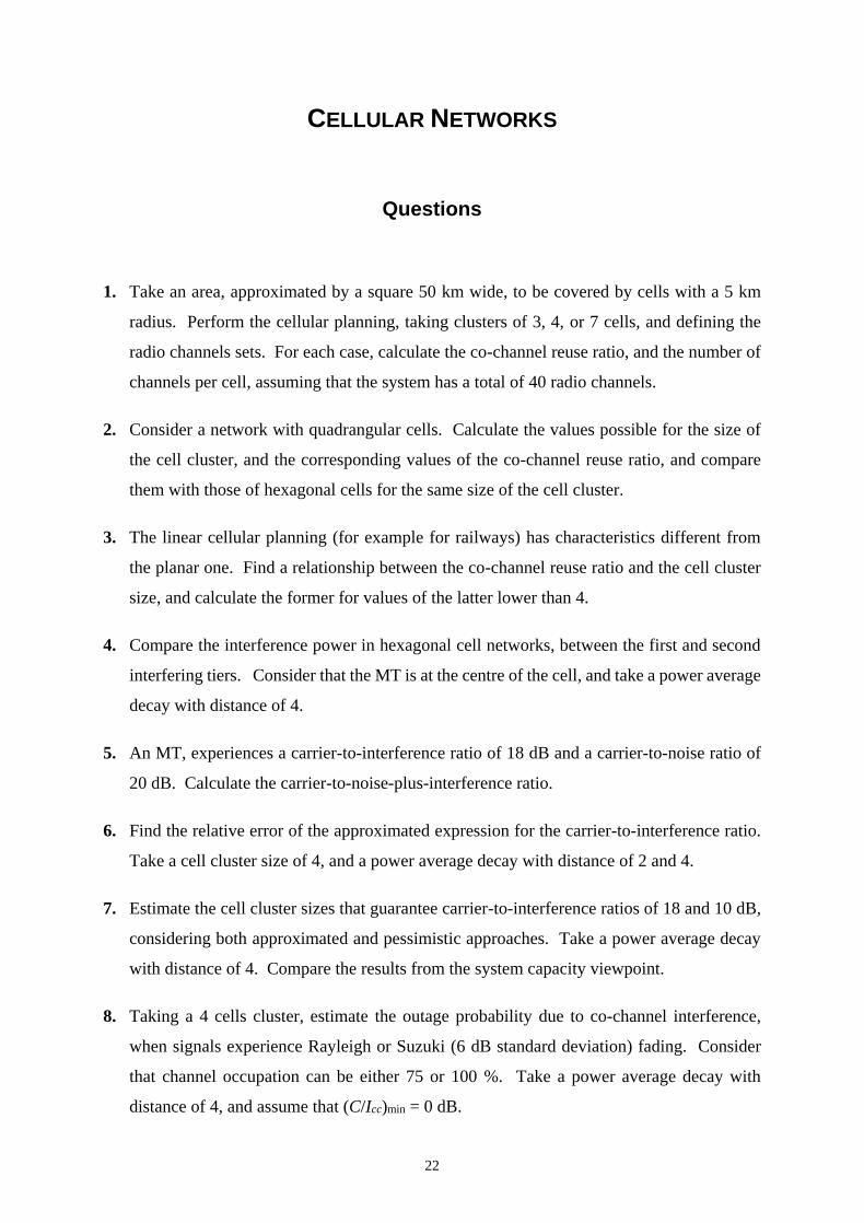
22
CELLULAR NETWORKS
Questions
1. Take an area, approximated by a square 50 km wide, to be covered by cells with a 5 km
radius. Perform the cellular planning, taking clusters of 3, 4, or 7 cells, and defining the
radio channels sets. For each case, calculate the co-channel reuse ratio, and the number of
channels per cell, assuming that the system has a total of 40 radio channels.
2. Consider a network with quadrangular cells. Calculate the values possible for the size of
the cell cluster, and the corresponding values of the co-channel reuse ratio, and compare
them with those of hexagonal cells for the same size of the cell cluster.
3. The linear cellular planning (for example for railways) has characteristics different from
the planar one. Find a relationship between the co-channel reuse ratio and the cell cluster
size, and calculate the former for values of the latter lower than 4.
4. Compare the interference power in hexagonal cell networks, between the first and second
interfering tiers. Consider that the MT is at the centre of the cell, and take a power average
decay with distance of 4.
5. An MT, experiences a carrier-to-interference ratio of 18 dB and a carrier-to-noise ratio of
20 dB. Calculate the carrier-to-noise-plus-interference ratio.
6. Find the relative error of the approximated expression for the carrier-to-interference ratio.
Take a cell cluster size of 4, and a power average decay with distance of 2 and 4.
7. Estimate the cell cluster sizes that guarantee carrier-to-interference ratios of 18 and 10 dB,
considering both approximated and pessimistic approaches. Take a power average decay
with distance of 4. Compare the results from the system capacity viewpoint.
8. Taking a 4 cells cluster, estimate the outage probability due to co-channel interference,
when signals experience Rayleigh or Suzuki (6 dB standard deviation) fading. Consider
that channel occupation can be either 75 or 100 %. Take a power average decay with
distance of 4, and assume that (C/Icc)min = 0 dB.

23
9. Calculate the gain in carrier-to-interference ratio from a tri-sector network to a non-sector
one, when using a 4 cells cluster, and taking a power average decay with distance of 4.
10. Consider a case of adjacent channel interference, where the interfering MT is closer to the
BS than the reference MT. Calculate the ratio between the distances of the two MTs to the
BS that leads to a difference in path loss equal to the filter isolation, when it has a
characteristic of 6, 12, and 24 dB/oct. Assume a power average decay with distance of 4,
and that radio channels separation is 6 times larger than the bandwidth.
11. Calculate the difference in path loss from two MTs 1 and 35 km away from the BS.
Consider power average decays with distance of 3 and 4. Comment on the results, from
the near-far interference viewpoint.
24
CELLULAR NETWORKS
Solutions
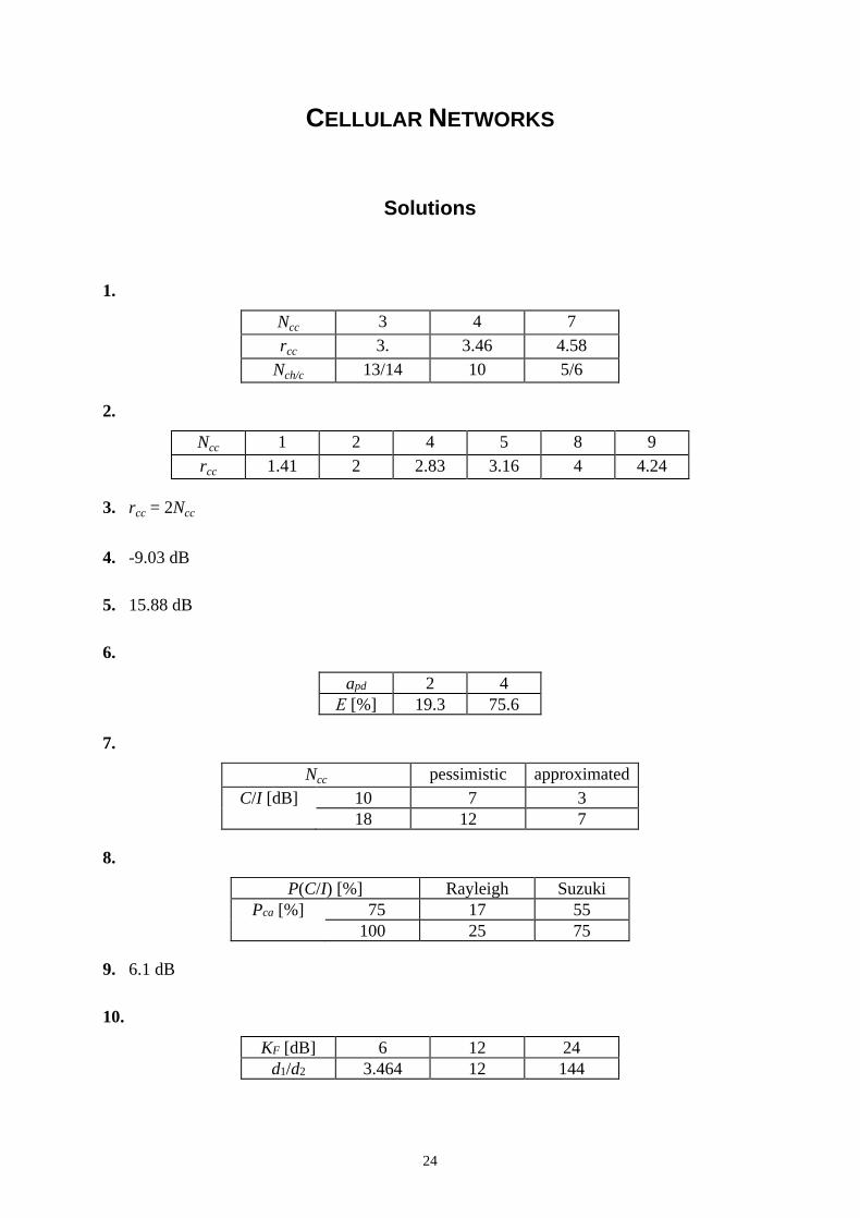
1.
Ncc 3 4 7
rcc 3. 3.46 4.58
Nch/c 13/14 10 5/6
2.
Ncc 1 2 4 5 8 9
rcc 1.41 2 2.83 3.16 4 4.24
3. rcc = 2Ncc
4. -9.03 dB
5. 15.88 dB
6.
apd 2 4
Ε [%] 19.3 75.6
7.
Ncc pessimistic approximated
C/I [dB] 10 7 3
18 12 7
8.
P(C/I) [%] Rayleigh Suzuki
Pca [%] 75 17 55
100 25 75
9. 6.1 dB
10.
KF [dB] 6 12 24
d1/d2 3.464 12 144

25
11.
apd 3 4
ΔLp [dB] 46.32 61.76

26
RADIO INTERFACE
Questions
1. Consider a UMTS user U1 to whom the code (1, 1, 1, 1) is allocated, receiving a signal
from another user U2 coded with (-1, 1, -1, 1). Is user U2 going to interfere with U1? Is
user U2 going to interfere with the other users in the cell?
2. Compare the GSM bit duration with the channel delay spread, in the two cases of the urban
environment, and comment on the result.
3. Analyse the capacity of the GSM 900 equaliser to compensate for the channel for MTs
moving at 4, 120 and 360 km/h, by comparing the time-slot duration with the coherence
time.
4. Calculate the distance corresponding to signal propagation during the guard time of a GSM
access burst, and compare with the nominal cell radius.
5. Take a MIMO system in which the number of transmitting and receiving antennas are equal,
and compare its maximum capacity with the equivalent SISO one.

27
RADIO INTERFACE
Solutions
1. No. Yes.
2.
Environment TU BU
Tbit/στ 3.767 1.459
3.
v [km/h] 4 120 360
Tc/TTS 90.590 3.020 1.007
4. 2.160
5. CMIMO = NT,R CSISO

28
MOBILITY AND TRAFFIC
Questions
1. Calculate the cell crossing rate and the handover ratio for cell radius of 1, 5, and 20 km,
assuming that MTs move at 4, 60, and 120 km/h, performing calls with an average duration
of 120 s.
2. Estimate the traffic offered to an urban micro-cell, with a 2 km radius, coming from vehicles
under the following conditions:
the cell is radially crossed by 2 motorways with 6 lanes, and 4 others with 4;
the average distance between cars, in a total jam situation, is 7 m;
the penetration ratio is 10 %;
the usage ratio is 50 %;
on average, each user makes 1 phone call per hour, with a 3 minutes duration.
3. A network with call blocking is under analysis, for an expected offered traffic of 50 Erl.
a) Calculate the number of traffic channels that allow the processing of the offered traffic
with a blocking of 2, 5 and 7 %.
b) Assuming that the network is designed for a blocking of 2 %, which would be the values
of the offered and transported traffic for a blocking of 5 and 7 %.
4. A PMR network with a 1.5 km radius cell, has 15 traffic channels with a waiting queue for
voice communications. On average, users make 1 phone call per hour, with a traffic of
0.029 Erl. Assuming that the delay probability is 5 %, calculate the user density (in
[user/km2]) that the network can process, and the probability that a call will wait more than
10 s.
5. In a PMR network with 20 traffic channels in a waiting queue for voice communications,
users make, on average, 2 calls per hour, with a 50 s duration. Assuming that the delay
probability is 3 %, calculate the number of users that can be processed, the average number
of calls in the waiting queue, and their average waiting time. Comment on the results.

29
6. Take a network for packet transmission, with 1 server of infinite capacity, in which packet
generation is described by the Poisson Distribution and duration by the Exponential one.
Find expressions for the average time that packets are in the system, and their average
number.
7. Take a network for packet transmission of the type M/M/1, in which packets arrive each
4 ms, having a 3 ms duration.
a) Calculate the average time that packets wait to be transmitted.
b) Calculate the average time that packets are in the system, and their average number.
c) Assuming that the average time that packets are in the system could be twice the one
previously calculated, what would be the corresponding percentage increase of the
packet arrival rate? Comment on the results.
8. An urban 1 km radius micro-cell covers a pedestrian area, where users (with speeds up to
4 km/h) make calls with a 90 s duration. After the installation in that area of a high speed
train railway (speeds up to 220 km/h), where passengers make calls with a 240 s duration,
the need for the deployment of a specific solution to cover the railway has to be analysed.
Calculate the handover probability for the two types of users, and comment on the results.
9. In an urban cell with a 2 km radius, users move with an average speed of 20 km/h, making
calls with a 100 s duration. Calculate the percentage of traffic due to handover.
10. A GSM network has a total of 60 radio channels. Compare the transported traffic, for a
2 % blocking, when cells have either an omnidirectional or a sector configuration, using in
both cases around 6 % of the physical channels for signalling and control.
11. A GSM 900 operator has a network with a total of 40 radio channels, and 20 km radius
cells in a rural area.
a) Compare the traffic transported by a BS, for a 1 % blocking, when either 1 or 2 physical
channels are taken for signalling and control. Do you consider this decision to be a
critical one in terms of QoS?
b) Compare, for the most unfavourable case of the previous question from the network
capacity viewpoint, the number of user processed by a BS, assuming that they make 1
call per hour with a 120 s duration.
c) Calculate the handover ratio under the conditions of maximum speed on a motorway.

30
12. Prove that:
a) the handover failure probability equals the blocking one, when no channels are reserved
for handover;
b) the handover failure probability is lower than the blocking one, when channels are
reserved for handover.

31
MOBILITY AND TRAFFIC
Solutions
1.
ηh [s-1] R [km]
1 5 20
4 8.17·10-4 1.63·10-4 4.08·10-5
v [km/h] 60 1.23·10-2 2.45·10-3 6.13·10-4
120 2.45·10-2 4.90·10-3 1.23·10-3
ξh R [km]
1 5 20
4 0.098 0.020 0.005
v [km/h] 60 1.470 0.294 0.074
120 2.940 0.588 0.147
2. 40 Erl
3. a)
PB [%] 2 5 7
NTCH 61 56 54
b)
PB [%] 5 7
T [Erl] 55.6 58.1
Ttrans [Erl] 52.82 54.03
4. 42.87 user/km2, 2.76 %
5. Nu = 457, del = 205.5 ms, delcallN = 0.052
6.
sa
ssys
1
,
sa
sasyspN
1
7. a) 9 ms
b) 12 ms, 3
c) 16.67 %
32
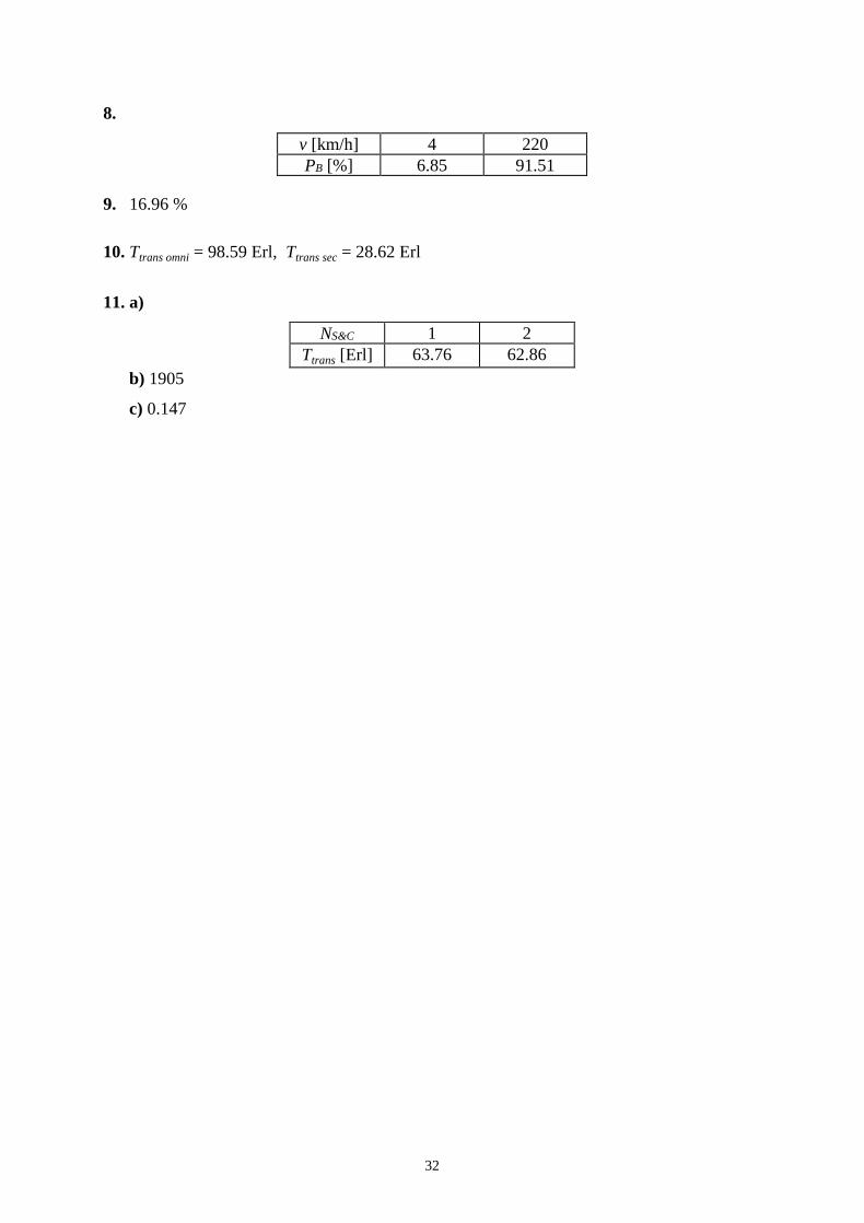
8.
v [km/h] 4 220
PB [%] 6.85 91.51
9. 16.96 %
10. Ttrans omni = 98.59 Erl, Ttrans sec = 28.62 Erl
11. a)
NS&C 1 2
Ttrans [Erl] 63.76 62.86
b) 1905
c) 0.147

33
CELLULAR DESIGN
Questions
1. Compare the receivers’ sensitivity between GSM and UMTS, for the voice service, under
the most favourable case, in UL and DL. Take, in UMTS, for UL, a maximum load factor
of 50 % and a receiver’s noise figure of 5 dB, and for DL, 70 % and 8 dB, respectively.
2. Find expressions for the UL and DL load factors in UMTS, when all users use the voice
service, and compare them.
3. Compare the pole capacities of UMTS (corresponding to load factors equal to 1) between
UL and DL, under the most favourable case and mono-service usage, by calculating the
number of users with either the voice or the 384 kb/s data services. Compare the obtained
values with the ones resulting from the maximum acceptable values for the load factors,
i.e., 50 and 70 %, respectively for UL and DL. Take 50 % for both the normalised inter-
cell interference and the code orthogonality factor.
34
CELLULAR DESIGN
Solutions
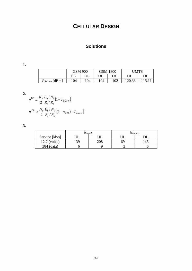
1.
GSM 900 GSM 1800 UMTS
UL DL UL DL UL DL
PRx min [dBm] -104 -104 -104 -102 -120.33 -115.11
2.
ninter
bc
buUL IRR
NEN 1
/
/
20
ninterCO
bc
buDL IRR
NEN 1
/
/
2
0
3.
Nu pole Nu max
Service [kb/s] UL UL UL DL
12.2 (voice) 139 208 69 145
384 (data) 6 9 3 6

35
LIST OF ACRONYMS
AFD Average Fade Duration
BS Base Station
CDF Cumulative Distribution Function
DL Downlink
EGC Equal Gain Combining
EIRP Effective Isotropic Radiated Power
ERPd Effective Radiated Power by half wavelength dipole
GSM Global System for Mobile Communications
LCR Level Crossing Rate
MRC Maximal Ratio Combining
MT Mobile Terminal
PDF Probability Density Function
PDP Power Delay Profile
PMR Private Mobile Radio
PSC Pure Selection Combining
QoS Quality of Service
Rx Receiver
SNR Signal-to-Noise Ratio
TSC Threshold Selection Combining
UL Uplink
UMTS Universal Mobile Telecommunications System
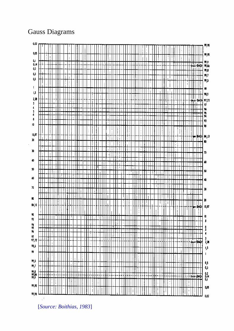
Gauss Diagrams
[Source: Boithias, 1983]

Suzuki CDF
[Fonte: ITU-R, Vol. V, Rep. 1007]
2/ xx
[Source: ITU-R, Vol. V, Rep. 1007]
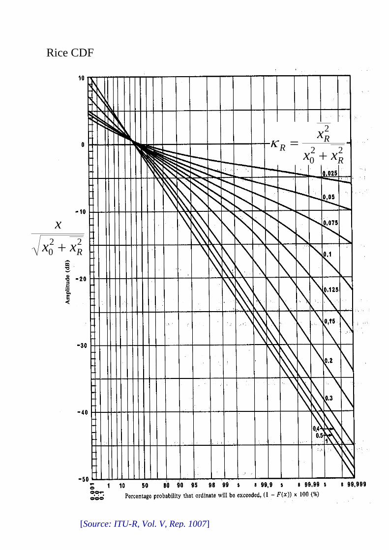
Rice CDF
220 Rxx
x
220
2
R
RR
xx
x
[Source: ITU-R, Vol. V, Rep. 1007]
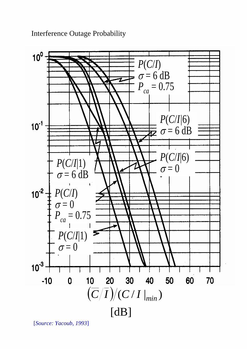
Interference Outage Probability
[dB]
)|/( minICIC
P(C/I) = 6 dBPca = 0.75
P(C/I|1) = 0
P(C/I|6) = 6 dB
P(C/I|6) = 0
P(C/I|1) = 6 dB
P(C/I) = 0Pca = 0.75
P(C/I) = 6 dBPca = 0.75
P(C/I|1) = 0
P(C/I|6) = 6 dB
P(C/I|6) = 0
P(C/I|1) = 6 dB
P(C/I) = 0Pca = 0.75
[Source: Yacoub, 1993]
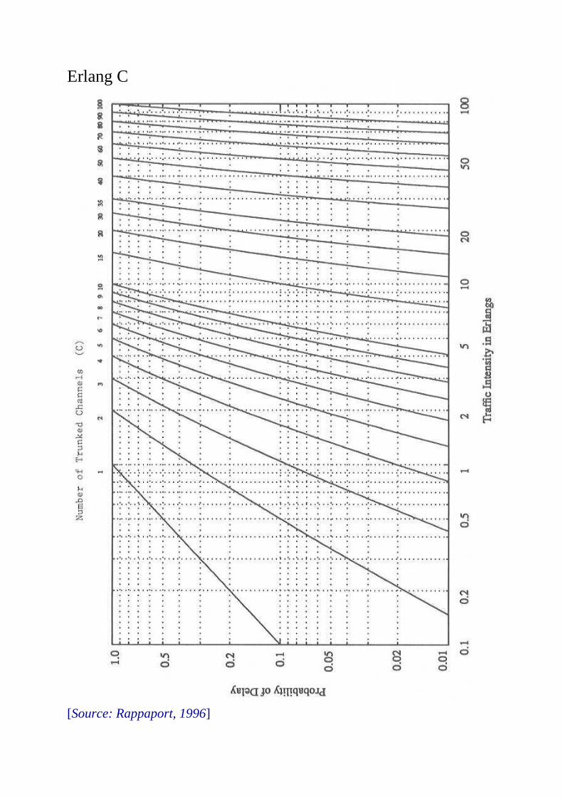
Erlang C
[Source: Rappaport, 1996]
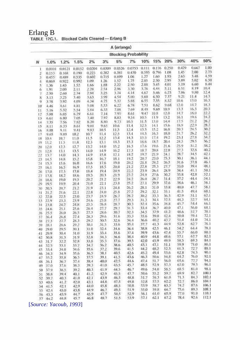
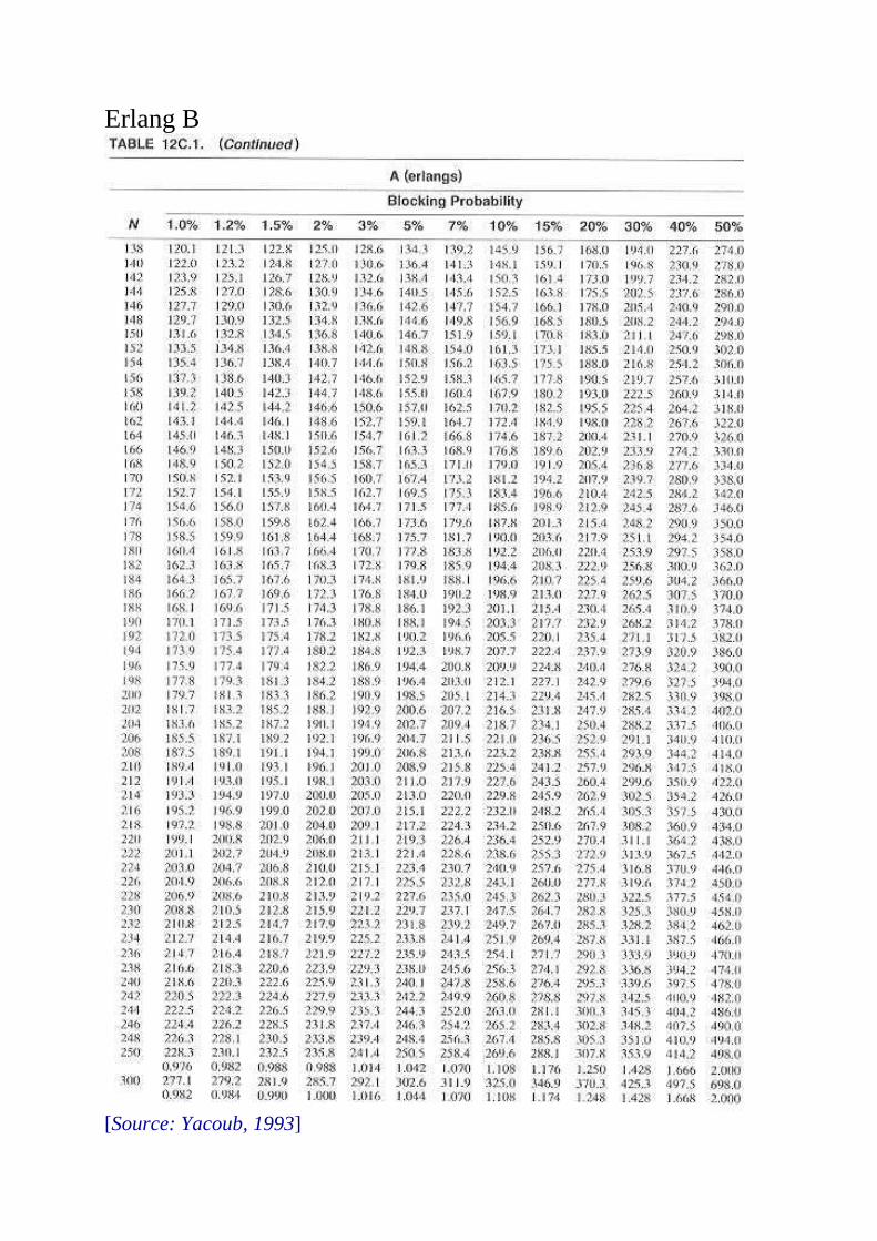
Erlang B
[Source: Yacoub, 1993]

Erlang B
[Source: Yacoub, 1993]
Erlang B
[Source: Yacoub, 1993]