A Basic Set of Homeostatic Controller Motifs T. Drengstig, † I. W. Jolma, ‡ X. Y. Ni, ‡ K. Thorsen, † X. M. Xu, ‡ and P. Ruoff ‡ * † Department of Electrical Engineering and Computer Science and ‡ Centre for Organelle Research, University of Stavanger, Stavanger, Norway ABSTRACT Adaptation and homeostasis are essential properties of all living systems. However, our knowledge about the reaction kinetic mechanisms leading to robust homeostatic behavior in the presence of environmental perturbations is still poor. Here, we describe, and provide physiological examples of, a set of two-component controller motifs that show robust homeostasis. This basic set of controller motifs, which can be considered as complete, divides into two operational work modes, termed as inflow and outflow control. We show how controller combinations within a cell can integrate uptake and metabolization of a homeostatic controlled species and how pathways can be activated and lead to the formation of alternative products, as observed, for example, in the change of fermentation products by microorganisms when the supply of the carbon source is altered. The antagonistic character of hormonal control systems can be understood by a combination of inflow and outflow controllers. INTRODUCTION Homeostasis is the concept that describes the coordinated physiological processes maintaining most of the steady states in organisms (1–3). Homeostasis does not necessarily imply a lack of change, but may include time-dependent behavior such as set-point changes or oscillatory responses (1,2). Alternative terminologies, such as predictive homeo- stasis (4,5), rheostasis (5,6), or allostasis (5,7), have been suggested to address these dynamic aspects of homeostatic control, and to emphasize the connection to adaptive and anticipatory functions of circadian rhythms together with the occurrence of orchestrated set-point changes. Common to all these homeostasis-related concepts is the presence of coordinated responses to maintain internal cellular and organismic stability (8). An important aspect of adaptive or homeostatic systems is their robustness (9–14), i.e., their ability to maintain functionality in the presence of various uncontrollable envi- ronmental disturbances. From a control-engineering per- spective, the concept of integral control leads to robust perfect adaptation (15). The use of integral control in homeostatic biological systems (16) was discussed by Saun- ders and colleagues (17,18) and its use in robust perfect adaptation of reaction kinetic networks has been demon- strated by Yi et al. (19) and others (20–23). We showed that the presence of zero-order kinetics in the degradation/ inhibition of the controller molecule in two-component negative feedback loops is a way to achieve integral control and robust homeostasis (21). As a continuation of our previous work (21), we present here, with physiological examples, a complete set of two-component homeostatic controller motifs and their division into inflow and outflow controllers. We identify parameters that influence the accu- racy of the controllers and determine how hierarchical homeostatic behaviors of combined controllers can lead to multiple steady-state levels corresponding to the different controllers’ set points. We show how controller combina- tions can integrate uptake and assimilation within a cell and may lead to pathway switching in terms of outflow con- trol, forming new products. Also, dysfunctional behavior, such as integral windup (15), has been found in single and combined controllers, and its possible biological signifi- cance in relation to disease is mentioned. COMPUTATIONAL METHODS Rate equations were solved numerically using MATLAB/SIMULINK and FORTRAN. For details, see the Supporting Material. To make notations simpler, concentrations of compounds are denoted by compound names without square brackets. Concentrations and rate constants are given in arbitrary units (a.u.) unless stated otherwise. RESULTS Basic set of homeostatic controller motifs The motifs we consider here consist of negative feedback loops with two species, A and E, both of which are being formed and turned over. In control theoretic terms, A is called the controlled variable, which is kept at a homeostatic level, whereas species E is the manipulated variable (MV). Fig. 1 a shows the (complete) set of eight two-component molecular representations of negative feedback loops between A and E (hereby called motifs or controllers). The systematic construction of the eight motifs is given in the Supporting Material. It should be noted that the negative feedback loops alone are not sufficient to provide homeostasis. Ni et al. (21) found that to achieve perturbation-independent homeostasis, the Submitted January 1, 2012, and accepted for publication September 25, 2012. *Correspondence: [email protected]Editor: Andre Levchenko. Ó 2012 by the Biophysical Society 0006-3495/12/11/2000/11 $2.00 http://dx.doi.org/10.1016/j.bpj.2012.09.033 2000 Biophysical Journal Volume 103 November 2012 2000–2010
Transcript
2000 Biophysical Journal Volume 103 November 2012 2000–2010
A Basic Set of Homeostatic Controller Motifs
T. Drengstig,† I. W. Jolma,‡ X. Y. Ni,‡ K. Thorsen,† X. M. Xu,‡ and P. Ruoff‡*†Department of Electrical Engineering and Computer Science and ‡Centre for Organelle Research, University of Stavanger,Stavanger, Norway
ABSTRACT Adaptation and homeostasis are essential properties of all living systems. However, our knowledge about thereaction kinetic mechanisms leading to robust homeostatic behavior in the presence of environmental perturbations is stillpoor. Here, we describe, and provide physiological examples of, a set of two-component controller motifs that show robusthomeostasis. This basic set of controller motifs, which can be considered as complete, divides into two operational work modes,termed as inflow and outflow control. We show how controller combinations within a cell can integrate uptake and metabolizationof a homeostatic controlled species and how pathways can be activated and lead to the formation of alternative products, asobserved, for example, in the change of fermentation products by microorganisms when the supply of the carbon source isaltered. The antagonistic character of hormonal control systems can be understood by a combination of inflow and outflowcontrollers.
INTRODUCTION
Homeostasis is the concept that describes the coordinatedphysiological processes maintaining most of the steadystates in organisms (1–3). Homeostasis does not necessarilyimply a lack of change, but may include time-dependentbehavior such as set-point changes or oscillatory responses(1,2). Alternative terminologies, such as predictive homeo-stasis (4,5), rheostasis (5,6), or allostasis (5,7), have beensuggested to address these dynamic aspects of homeostaticcontrol, and to emphasize the connection to adaptive andanticipatory functions of circadian rhythms together withthe occurrence of orchestrated set-point changes. Commonto all these homeostasis-related concepts is the presenceof coordinated responses to maintain internal cellular andorganismic stability (8).
An important aspect of adaptive or homeostatic systemsis their robustness (9–14), i.e., their ability to maintainfunctionality in the presence of various uncontrollable envi-ronmental disturbances. From a control-engineering per-spective, the concept of integral control leads to robustperfect adaptation (15). The use of integral control inhomeostatic biological systems (16) was discussed by Saun-ders and colleagues (17,18) and its use in robust perfectadaptation of reaction kinetic networks has been demon-strated by Yi et al. (19) and others (20–23). We showedthat the presence of zero-order kinetics in the degradation/inhibition of the controller molecule in two-componentnegative feedback loops is a way to achieve integral controland robust homeostasis (21). As a continuation of ourprevious work (21), we present here, with physiologicalexamples, a complete set of two-component homeostaticcontroller motifs and their division into inflow and outflow
Submitted January 1, 2012, and accepted for publication September 25,
controllers. We identify parameters that influence the accu-racy of the controllers and determine how hierarchicalhomeostatic behaviors of combined controllers can lead tomultiple steady-state levels corresponding to the differentcontrollers’ set points. We show how controller combina-tions can integrate uptake and assimilation within a celland may lead to pathway switching in terms of outflow con-trol, forming new products. Also, dysfunctional behavior,such as integral windup (15), has been found in single andcombined controllers, and its possible biological signifi-cance in relation to disease is mentioned.
COMPUTATIONAL METHODS
Rate equations were solved numerically using MATLAB/SIMULINK and
FORTRAN. For details, see the Supporting Material. To make notations
simpler, concentrations of compounds are denoted by compound names
without square brackets. Concentrations and rate constants are given in
arbitrary units (a.u.) unless stated otherwise.
RESULTS
Basic set of homeostatic controller motifs
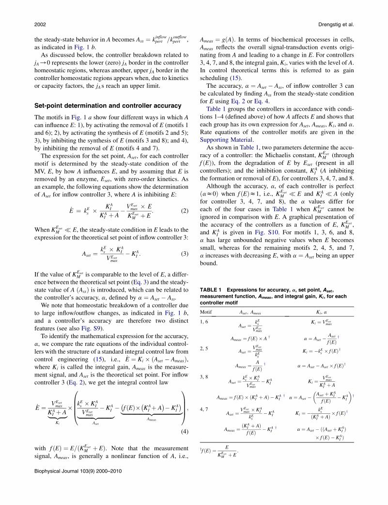
The motifs we consider here consist of negative feedbackloops with two species, A and E, both of which are beingformed and turned over. In control theoretic terms,A is calledthe controlled variable, which is kept at a homeostaticlevel, whereas species E is the manipulated variable (MV).Fig. 1 a shows the (complete) set of eight two-componentmolecular representations of negative feedback loopsbetween A and E (hereby called motifs or controllers). Thesystematic construction of the eight motifs is given in theSupporting Material.
It should be noted that the negative feedback loops aloneare not sufficient to provide homeostasis. Ni et al. (21) foundthat to achieve perturbation-independent homeostasis, the
steady state behavior of A foroivahebetatsydaetssrellortnocwolfnini A in outflow controllers
kpertinflow
kpertoutflow
Ass
0 5 10 15 20 25 30 35 40 45 50
05 10 15 20 25 30 35 40 45 50
1.0
0.8
0.6
1.0
0.4
0.2
a
b
FIGURE 1 A complete set of two-component homeostatic controller motifs. (a) The motifs fall into two operational classes termed inflow and outflow
controllers (for definition, see main text). Each motif is able to show robust homeostasis in Awhen the MV, E, is subject to removal by zero-order kinetics.
(b) Figures show the steady-state values of A for inflow and outflow controllers as a function of kinflowpert and koutflowpert , respectively, with Ainset ¼ Aout
set ¼ 1. Typi-
cally, the homeostatic behavior of all inflow controllers breaks down when inflow perturbations become dominant (Ass levels rise above Aset ; left), whereas
for outflow controllers, homeostasis breakdown is observed when outflow perturbations from A become dominant (Ass levels decrease below Aset ; right). At
these breakdowns, the compensatory flux, jA (Eq. 1), is zero, which defines the lower borders of the controller homeostatic regions.
Homeostatic Controller Motifs 2001
removal of E by zero-order kinetics (due to an enzyme, Eset)is a sufficient condition. We will show below that underthese zero-order kinetic conditions, integral control is oper-ational, where the level of E is proportional to the integratederror between A and set point Aset.
Four of themotifs in Fig. 1were published previously (21),and Yi et al. (19) gave the first example of motif 2 exhibitingrobust homeostasis by including zero-order removal of theMV, but without mentioning the importance of zero-orderkinetics in obtaining integral control. Here, we describefour additional motifs, which makes the set complete.
Closer inspection of the motifs shows that the set dividesequally into two operational classes recognized in ourprevious work (21) and termed inflow and outflow control-lers. However, inflow controllers are here redefined as main-taining homeostasis by adding A to the system from an
internal or environmental source, whereas outflow control-lers maintain homeostasis by removing A from the system.
The dynamics of A can be written as
_A ¼ kinflowpert � koutflowpert � A5 jA; (1)
where kinflowpert and koutflowpert are parameters related to uncon-trolled inflow/outflow perturbations, and jA is theE-mediatedcompensatory flux, which adds A to or removes it from thesystem by inflow or outflow controllers, respectively.
As emphasized previously (21), the homeostatic behaviorof inflow controllers breaks down when there are largeuncontrolled inflows, whereas outflow controllers lose theirhomeostatic behavior in the presence of large uncontrolledoutflows. At these breakdowns, the E-mediated compensa-tory fluxes ðjAÞ of added or removed A become zero, and
Biophysical Journal 103(9) 2000–2010
2002 Drengstig et al.
the steady-state behavior in A becomes Ass ¼ kinflowpert =koutflowpert ,as indicated in Fig. 1 b.
As discussed below, the controller breakdown related tojA/0 represents the lower (zero) jA border in the controllerhomeostatic regions, whereas another, upper jA border in thecontroller homeostatic regions appears when, due to kineticsor capacity factors, the jA s reach an upper limit.
Set-point determination and controller accuracy
The motifs in Fig. 1 a show four different ways in which Acan influence E: 1), by activating the removal of E (motifs 1and 6); 2), by activating the synthesis of E (motifs 2 and 5);3), by inhibiting the synthesis of E (motifs 3 and 8); and 4),by inhibiting the removal of E (motifs 4 and 7).
The expression for the set point, Aset, for each controllermotif is determined by the steady-state condition of theMV, E, by how A influences E, and by assuming that E isremoved by an enzyme, Eset, with zero-order kinetics. Asan example, the following equations show the determinationof Aset for inflow controller 3, where A is inhibiting E:
_E ¼ kEs � KAI
KAI þ A
� VEsetmax � E
KEsetM þ E
: (2)
When KEset
M � E, the steady-state condition in E leads to the
TABLE 1 Expressions for accuracy, a, set point, Aset ,
measurement function, Ameas , and integral gain, Ki , for each
controller motif
Motif Aset; Ameas Ki, a
1, 6Aset ¼ kEs
VEsetmax
Ki ¼ VEsetmax
Ameas ¼ f ðEÞ � A y a ¼ Aset � Aset
f ðEÞy
2, 5 Aset ¼ VEsetmax
kEsKi ¼ �kEs � f ðEÞy
Ameas ¼ A
f ðEÞy
a ¼ Aset � Aset � f ðEÞy
3, 8Aset ¼ kEs � KA
I
VEsetmax
� KAI Ki ¼ VEset
max
KAI þ A
Ameas ¼ f ðEÞ � ðKAI þ AÞ � KA
Iy
a ¼ Aset ��Aset þ KA
I
f ðEÞ � KAI
�y
4, 7Aset ¼ VEset
max � KAI
kEs� KA
I Ki ¼ � kEsðKA
I þ AÞ � f ðEÞy
Ameas ¼ ðKAI þ AÞf ðEÞ � KA
Iy a ¼ Aset � ððAset þ KA
I Þ� f ðEÞ � KA
I Þyf ðEÞ ¼ E
KEset
M þ E.
expression for the theoretical set point of inflow controller 3:
Aset ¼ kEs � KAI
VEsetmax
� KAI : (3)
If the value of KEset
M is comparable to the level of E, a differ-ence between the theoretical set point (Eq. 3) and the steady-state value of A ðAssÞ is introduced, which can be related tothe controller’s accuracy, a, defined by a ¼ Aset � Ass.
We note that homeostatic breakdown of a controller dueto large inflow/outflow changes, as indicated in Fig. 1 b,and a controller’s accuracy are therefore two distinctfeatures (see also Fig. S9).
To identify the mathematical expression for the accuracy,a, we compare the rate equations of the individual control-lers with the structure of a standard integral control law fromcontrol engineering (15), i.e., _E ¼ Ki � ðAset � AmeasÞ,where Ki is called the integral gain, Ameas is the measure-ment signal, and Aset is the theoretical set point. For inflowcontroller 3 (Eq. 2), we get the integral control law
M þ EÞ. Note that the measurementsignal, Ameas, is generally a nonlinear function of A, i.e.,
Biophysical Journal 103(9) 2000–2010
Ameas ¼ gðAÞ. In terms of biochemical processes in cells,Ameas reflects the overall signal-transduction events origi-nating from A and leading to a change in E. For controllers3, 4, 7, and 8, the integral gain, Ki, varies with the level of A.In control theoretical terms this is referred to as gainscheduling (15).
The accuracy, a ¼ Aset � Ass, of inflow controller 3 canbe calculated by finding Ass from the steady-state conditionfor E using Eq. 2 or Eq. 4.
Table 1 groups the controllers in accordance with condi-tions 1–4 (defined above) of how A affects E and shows thateach group has its own expression for Aset, Ameas, Ki, and a.Rate equations of the controller motifs are given in theSupporting Material.
As shown in Table 1, two parameters determine the accu-racy of a controller: the Michaelis constant, KEset
M (throughf ðEÞ), from the degradation of E by Eset (present in allcontrollers); and the inhibition constant, KA
I (A inhibitingthe formation or removal of E), for controllers 3, 4, 7, and 8.
Although the accuracy, a, of each controller is perfectðaz0Þ when f ðEÞz1, i.e., KEset
M � E and KAI � A (only
for controller 3, 4, 7, and 8), the a values differ foreach of the four cases in Table 1 when KEset
M cannot beignored in comparison with E. A graphical presentation ofthe accuracy of the controllers as a function of E, KEset
M ,and KA
I is given in Fig. S10. For motifs 1, 3, 6, and 8,a has large unbounded negative values when E becomessmall, whereas for the remaining motifs 2, 4, 5, and 7,a increases with decreasing E, with a ¼ Aset being an upperbound.
Homeostatic Controller Motifs 2003
Performance of individual controllers
We considered the question of what factors will influencethe homeostatic regions when controllers have the sameaccuracies and set points.
If no restrictions are made on the concentrations in E andon the inflow/outflow compensatory fluxes, jA, all eightcontrollers show identical regions of homeostasis, onlylimited by the lower jA flux border of the controllers, as indi-cated in Fig. 1 b. However, differences in controller perfor-mances occur when the compensatory fluxes, jA, becomelimited due to either different capacities of the differentcontrollers to generate E or differences in the kinetics ofthe E-induced jA fluxes.
To illustrate the influence of jA limitation on homeostaticperformance, we chose for each controller a set pointof 2.0 a.u. and a maximum compensating flux of jA;max ¼10 a.u. To achieve this, the VEtr
max parameters for controllers1, 3, 5, and 7 were chosen such that jA;max ¼ 10 is obtainedat a maximum level of Emax ¼ 20, whereas for the E-inhib-iting controllers, jA;max ¼ 10 is obtained when E/0. Notethat the E-activated fluxes, jA, in controllers 1, 3, 5, and 7are first-order with respect to E, whereas the jA fluxes dueto E inhibition (controllers 2, 4, 6, and 8) show saturationkinetics, i.e., jA ¼ jA;max � KE
I =ðKEI þ EÞ (see derivation
of jA in the Supporting Material, Eq. S12). As will beshown below, these differences between E-activating and
kpertkpert
kpert
24
6
12345671.41.61.82
2.22.42.62.8
Ass
24
6
1234567
5
10
15
20 Ess
Ess
24
6
1234567
2
4
6
8
10
j A,ss
j A,ss
246810
1
2
3
As
246810
5
10
15
20
Ess
Ess
246810
2
4
6
8
j A
Assin,1
in,2
in,1
in,2
in,1
in,2
o
out,6
out,5
o
a
c
e
b
d
f
10
kpert
kpertkpert
kpertkpert
kpert
E-inhibiting jA kinetics will lead to different controllerperformance.
When comparing Ass levels between controllers, wefound that all E-activating controllers (1, 3, 5, and 7)behaved practically identically, as did all E-inhibitingcontrollers (2, 4, 6, and 8). However, when comparingE-inhibiting controllers with E-activating controllers, theE-inhibiting controllers performed less well at low KE
I
values than did the E-activating controllers. As an example,Fig. 2 shows the steady-state values of A, E, and jA forcontrollers 1 and 2 and controllers 5 and 6. E-activatingcontrollers 1 and 5 (Fig. 2, red) can maintain their homeo-static steady states in A as long as jA< jA;max. OncejA/jA;max ¼ 10 the upper border of the homeostatic regionis reached and homeostasis breaks down. For low KE
I values,the jA fluxes of E-inhibiting controllers 2 and 6 (Fig. 2, blue)are not large enough to compensate for the applied outflowperturbation, and their homeostatic performance is poorcompared to the E-activating controllers. However, at largerKEI and jA;max values, the performance of the E-inhibiting
controllers can match the performance of the E-activatingcontrollers.
On the other hand, when the first-order kinetics withrespect to E in the E-activating controllers is replaced bysaturation kinetics, i.e., jA ¼ jA;max � E=ðKE
a þ EÞ, then, asfor the E-inhibiting controllers (Fig. 2), the homeostaticperformance is dependent on the value of KE
a and is limited
kpert
510
1520
s
Ass
510
1520
510
1520
,ss
j A,ss
ut,5
out,6
ut,6
out,5
kpert
kpertFIGURE 2 Controller comparisons. (a, c, and e)
Behaviors of E-activating and E-inhibiting inflow
controllers 1 and 2 with respect to the steady-state
levels of A and E and the E-mediated inflow of A
and jA. Inflow controllers 3 and 4 show practically
identical behaviors (data not shown). (b, d, and f)
Behaviors of activating and inhibiting outflow
controllers 5 and 6 with respect to the steady-state
levels of A and E and the E-mediated outflow of A
and jA. Outflow controllers 7 and 8 show almost
identical behavior (data not shown). See also
Fig. S6 and Fig. S7 and the Supporting Material
description of how jA kinetics can influence
controller performance.
Biophysical Journal 103(9) 2000–2010
2004 Drengstig et al.
by the maximum compensatory flux jA;max (see SupportingMaterial for derivation of jA expression (Eq. S8) and details(Fig. S7)). Thus, the homeostatic performance of thecontrollers depends largely on the kinetics of the compensa-tory flux, jA, and its limits and not on the negative feedbackstructure of the controller motif.
Controllers’ hierarchical dominance
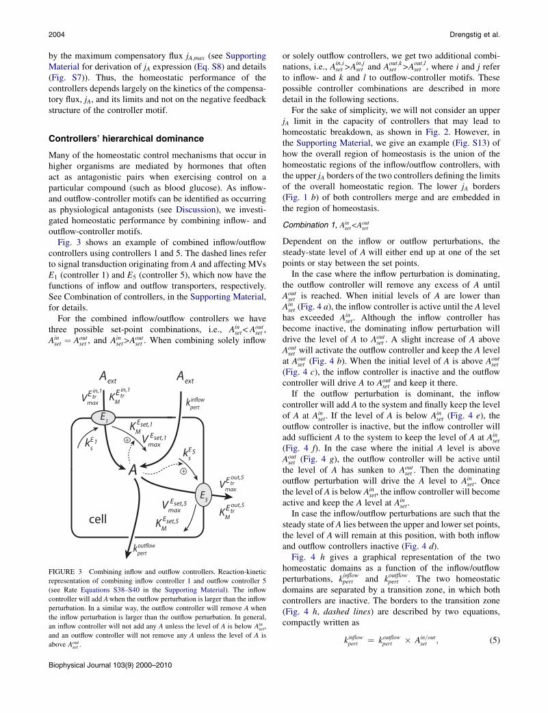
Many of the homeostatic control mechanisms that occur inhigher organisms are mediated by hormones that oftenact as antagonistic pairs when exercising control on aparticular compound (such as blood glucose). As inflow-and outflow-controller motifs can be identified as occurringas physiological antagonists (see Discussion), we investi-gated homeostatic performance by combining inflow- andoutflow-controller motifs.
Fig. 3 shows an example of combined inflow/outflowcontrollers using controllers 1 and 5. The dashed lines referto signal transduction originating from A and affecting MVsE1 (controller 1) and E5 (controller 5), which now have thefunctions of inflow and outflow transporters, respectively.See Combination of controllers, in the Supporting Material,for details.
For the combined inflow/outflow controllers we havethree possible set-point combinations, i.e., Ain
set< Aoutset ,
Ainset ¼ Aout
set , and Ainset>A
outset . When combining solely inflow
+
A
E1
+
ksE5
KM Eset,1
Vmax Eset,1ks
E1
Vmax Eset,5
KM Eset,5
kpert
kpert
E5
Vmax Etr
out,5
KM Etr
out,5
KM Etr
in,1
Vmax Etr
in,1
Aext Aext
cell
FIGURE 3 Combining inflow and outflow controllers. Reaction-kinetic
representation of combining inflow controller 1 and outflow controller 5
(see Rate Equations S38–S40 in the Supporting Material). The inflow
controller will add Awhen the outflow perturbation is larger than the inflow
perturbation. In a similar way, the outflow controller will remove A when
the inflow perturbation is larger than the outflow perturbation. In general,
an inflow controller will not add any A unless the level of A is below Ainset,
and an outflow controller will not remove any A unless the level of A is
above Aoutset .
Biophysical Journal 103(9) 2000–2010
or solely outflow controllers, we get two additional combi-nations, i.e., Ain;i
set >Ain;jset and Aout;k
set >Aout;lset , where i and j refer
to inflow- and k and l to outflow-controller motifs. Thesepossible controller combinations are described in moredetail in the following sections.
For the sake of simplicity, we will not consider an upperjA limit in the capacity of controllers that may lead tohomeostatic breakdown, as shown in Fig. 2. However, inthe Supporting Material, we give an example (Fig. S13) ofhow the overall region of homeostasis is the union of thehomeostatic regions of the inflow/outflow controllers, withthe upper jA borders of the two controllers defining the limitsof the overall homeostatic region. The lower jA borders(Fig. 1 b) of both controllers merge and are embedded inthe region of homeostasis.
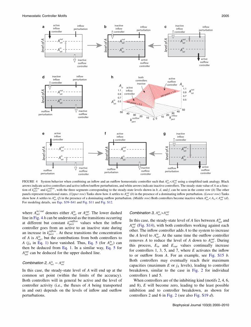
Combination 1, Ainset<A
outset
Dependent on the inflow or outflow perturbations, thesteady-state level of A will either end up at one of the setpoints or stay between the set points.
In the case where the inflow perturbation is dominating,the outflow controller will remove any excess of A untilAoutset is reached. When initial levels of A are lower than
Ainset (Fig. 4 a), the inflow controller is active until the A level
has exceeded Ainset. Although the inflow controller has
become inactive, the dominating inflow perturbation willdrive the level of A to Aout
set . A slight increase of A aboveAoutset will activate the outflow controller and keep the A level
at Aoutset (Fig. 4 b). When the initial level of A is above Aout
set
(Fig. 4 c), the inflow controller is inactive and the outflowcontroller will drive A to Aout
set and keep it there.If the outflow perturbation is dominant, the inflow
controller will add A to the system and finally keep the levelof A at Ain
set. If the level of A is below Ainset (Fig. 4 e), the
outflow controller is inactive, but the inflow controller willadd sufficient A to the system to keep the level of A at Ain
set
(Fig. 4 f). In the case where the initial A level is aboveAoutset (Fig. 4 g), the outflow controller will be active until
the level of A has sunken to Aoutset . Then the dominating
outflow perturbation will drive the A level to Ainset. Once
the level of A is below Ainset, the inflow controller will become
active and keep the A level at Ainset.
In case the inflow/outflow perturbations are such that thesteady state of A lies between the upper and lower set points,the level of A will remain at this position, with both inflowand outflow controllers inactive (Fig. 4 d).
Fig. 4 h gives a graphical representation of the twohomeostatic domains as a function of the inflow/outflowperturbations, kinflowpert and koutflowpert . The two homeostaticdomains are separated by a transition zone, in which bothcontrollers are inactive. The borders to the transition zone(Fig. 4 h, dashed lines) are described by two equations,compactly written as
kinflowpert ¼ koutflowpert � Ain=outset ; (5)
leve
l of A
inactive
controller
inactive
controller
leve
l of A
active
controller
inactive
controller
perturbation
leve
l of A
inactive
controller
active
controller
leve
l of A
inactive
controller
active
controller
0 10
20 30
40 50
0 10 20 30 40 50
0.5
0.7
0.9
1.1
0.5
0.7
0.9
1.1
kpertkpert
AssAss
active
controller
set-point = 1.0
set-point = 0.5
active
controller
both controllers
inactive
Aset
in
Aset
out
Aset
in
Aset
out
Aset
in
Aset
out
Aset
in
Aset
out
leve
l of A
active
controller
inactive
controller
leve
l of A
inactive
controller
active
controller
leve
l of A
active
controller
inactive
controller
Aset
in
Aset
out
Aset
in
Aset
out
Aset
in
Aset
out
Aset
in
Aset
out
perturbationperturbation
perturbation
perturbation perturbation perturbation
cba
d
e f g
h
perturbation
FIGURE 4 System behavior when combining an inflow and an outflow homeostatic controller such that Ainset<A
outset using a simplified tank analogy. Black
arrows indicate active controllers and active inflow/outflow perturbations, and white arrows indicate inactive controllers. The steady-state value of A as a func-
tion of kinflowpert and koutflowpert , with the three segments corresponding to the steady-state levels shown in b, d, and f, can be seen in the center row (h) The other
panels represent transitional states. (Upper row) Tanks show how A settles to Aoutset (b) in the presence of a dominating inflow perturbation. (Lower row) Tanks
show how A settles to Ainset (f) in the presence of a dominating outflow perturbation. (Middle row) Both controllers become inactive when Ain
set< Ass< Aoutset (d).
For modeling details, see Eqs. S39–S41 and Fig. S11 and Fig. S12.
Homeostatic Controller Motifs 2005
where Ain=outset denotes either Ain
set or Aoutset . The lower dashed
line in Fig. 4 h can be understood as the transitions occurringat different but constant koutflowpert values when the inflowcontroller goes from an active to an inactive state duringan increase in kinflowpert . At these transitions the concentrationof A is Ain
set, but the contributions from both controllers toA (jA in Eq. 1) have vanished. Thus, Eq. 5 (for Ain
set) canthen be deduced from Eq. 1. In a similar way, Eq. 5 forAoutset can be deduced for the upper dashed line.
Combination 2, Ainset ¼ Aout
set
In this case, the steady-state level of A will end up at thecommon set point (within the limits of the accuracy).Both controllers will in general be active and the level ofcontroller activity (i.e., the fluxes of A being transportedin and out) depends on the levels of inflow and outflowperturbations.
Combination 3, Ainset>A
outset
In this case, the steady-state level of A lies between Ainset and
Aoutset (Fig. S14), with both controllers working against each
other. The inflow controller adds A to the system to increasethe A level to Ain
set. At the same time the outflow controllerremoves A to reduce the level of A down to Aout
set . Duringthis process, Ein and Eout values continually increasefor controllers 1, 3, 5, and 7, where E activates the inflowto or outflow from A. For an example, see Fig. S15 b.Both controllers may eventually reach their maximumcapacities (maximum E or jA levels), leading to controllerbreakdown, similar to the case in Fig. 2 for individualcontrollers 1 and 5.
When controllers are of the inhibiting kind (motifs 2, 4, 6,and 8), E will become zero, leading to the least possibleinhibition and to controller breakdown, as shown forcontrollers 2 and 6 in Fig. 2 (see also Fig. S19 d).
Biophysical Journal 103(9) 2000–2010
2006 Drengstig et al.
Although for this combination no distinct set points canbe observed for different kinflowpert and koutflowpert values (seeFig. S14), the location of the A steady state between Ain
set
and Aoutset depends on the parameters of the individual
controllers. For example, when the dominance of theoutflow controller is very low (V
Eouttr
max is low relative toVEintr
max), then the inflow controller determines the steady stateof A (see Fig. S14 a). By successively increasing the V
Eouttr
max ofthe outflow controller, the steady state in A changes gradu-ally toward Aout
set , see Fig. S14 c.
Combination 4, Ain;iset >A
in;jset
Combining two inflow controllers, i and j (assuming a highuncontrolled outflow in A), controller i, with the higher setpoint, is active and determines the set point, whereascontroller j, with the lower set point, is inactive (Fig. S17).
Combination 5, Aout;kset >Aout;l
set
When combining two outflow controllers, k and l (assuminga high uncontrolled inflow in A), controller l, with the lowerset point, will dominate and determine the A value.Controller k, with the higher set point, is inactive, becausethe level of A is lower than Aout;k
set and there is no need forcontroller k to remove more A.
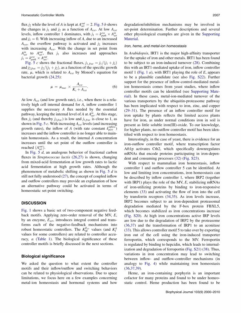
Activating pathways
Using Combination 1 between an inflow and an outflowcontroller, the activation of the outflow controller pathwayis observed when an (uncontrolled) inflow of A into a cell
+
uncontrolled
A
a
c
E5
E1
controlled
0
0.2
0.4
0.6
0.8
1
0 0.1 0.2 0.3 0.4
fract
ion
of c
arbo
n flu
xes
specific growth
mixed acid fermentation
d
+
j2
0
0.2
0.4
0.6
0.8
1
1
1.2
1.4
1.6
1.8
2
0 0.1 0.2 0.3 0.4 0.5 0.6 0.7 0.8
internal concentration of A, a.u.
fract
ion
of fl
uxes
j 1 and
j 2
specific growth rate µ, a.u
internal A
j2,frac
j1,frac
kpert
VmaxEtr
out
KMEtr
out
ksE5
KMEset,5
VmaxEset,5
ksE1
KMEtr
inVmax
Etrin
Aext
VmaxEset,1
KMEset,1
kpathess
j1
pathway
essentialpathway
b
0 10 20 30 400.5
0.6
0.7
0.8
0.9
1
1.1
1.2
1.3
0 10 20 30 40concentration o
j1
flux j 1
cell
Biophysical Journal 103(9) 2000–2010
becomes dominant. In Fig. 4 f, a sudden dominating inflowperturbation will lead to a change from inflow control tooutflow control (Fig. 4 b) via the transition zone (Fig. 4 d).In addition, a change (increase) in the steady-state concen-tration of A from Ain
set to Aoutset will be observed. In terms of
outflow control, two situations can be considered, one inwhich excess of A is transported out of the cell (excreted),as in Fig. 3, or one in which the excess of environmentallytaken up A (environmental concentration of A is denotedAext) is transformed into one or several products within thecell by an overflow pathway (with flux j2) (Fig. 5 a). InFig. 5 a, A can enter the cell by an uncontrolled (diffusion-like) first-order mechanism with flux kinflowpert � Aext and byinflow controller 1, where the manipulated variable E1 playsthe role of the transporter with set point Ain
set ¼ 1. The over-flow pathway is regulated by outflow-controller motif 5,where the manipulated variable E5 plays the role of anenzyme converting A into another product. The overflowpathway has a set point of Aout
set ¼ 2. In the absence of an
uncontrolled inflow of A (kinflowpert ¼ 0 in Fig. 5 a), the level
of A is determined by inflow controller 1 with Ainset ¼ 1,
and all A is directed into the essential pathway with fluxj1. Typically, for inflow controllers, transporter E1 willdeliver to the essential pathway only as much A as is needed(which may depend on environmental conditions). At theseconditions, the overflow pathway is shut off. However, whenan additional large inflow of A occurs, the concentration ofAwithin the cell increases until the set point of the outflowcontroller is exceeded. At that stage, the outflow controlleris activated and removes excess of A by enzyme E5 with
0.5 0.6 0.7 0.8
rate, h-1
lactic acid fermentation
50 60 70 8050 60 70 800
2
4
6
8
10
12
14
16
f Aext, a.u.
flux j 2
j2
FIGURE 5 Illustration of pathway activation
by a combination of inflow 1 and outflow 5 control-
lers. (a) Excess of A can be handled by a cell-
internal overflow pathway with flux j2. (b)
Induction of the overflow pathway when a large
inflow of A enters the cell, leading to an increase
in fluxes j1 and j2. Rate-constant values are given
in Activated pathways in the Supporting Material.
(c) Calculated fractional fluxes j1;frac and j2;fracfrom b together with the internal concentration of
A as a function of the specific growth rate, m. (d)
Experimentally observed shift of metabolic path-
ways in Streptococcus lactis from mixed-acid
production at low growth rates to lactic acid
production at high growth rates. Replotted from
Fig. 4 c of Molenaar et al. (27).
Homeostatic Controller Motifs 2007
flux j2 while the level of A is kept at Aoutset ¼ 2. Fig. 5 b shows
the changes in j1 and j2 as a function of Aext. At low Aext
and j2 ¼ 0. With increasing inflow of A, due to an increasedAext, the overflow pathway is activated and j2 increaseswith increasing Aext. With the change in set point fromAinset to Aout
set , flux j1 also increases and approachesj1 ¼ kesspath � Aout
set .Fig. 5 c shows the fractional fluxes, j1; frac ¼ j1=ðj1 þ j2Þ
and j2;frac ¼ j2=ðj1 þ j2Þ, as a function of the specific growthrate, m, which is related to Aext by Monod’s equation forbacterial growth (24,25):
m ¼ mmax � Aext
Ks þ Aext
: (6)
At low Aext (and low growth rate), i.e., when there is a rela-tively high cell internal demand for A, inflow controller 1supplies the necessary A flux needed by the essentialpathway, keeping the internal level of A at Ain
set. At this stage,flux j2 (and thereby j2;frac) is low and j1;frac is close to 1, asshown in Fig. 5 c. With increasing Aext levels (and increasinggrowth rates), the inflow of A (with rate constant kinflowpert )increases and the inflow controller is no longer able to main-tain homeostasis. As a result, the internal A concentrationincreases until the set point of the outflow controller isreached ðAout
set Þ.In Fig. 5 d, an analogous behavior of fractional carbon
fluxes in Streptococcus lactis (26,27) is shown, changingfrom mixed-acid fermentation at low growth rates to lacticacid fermentation at high growth rates. Although thephenomenon of metabolic shifting as shown in Fig. 5 d isstill not fully understood (27), the concept of coupled inflowand outflow controllers may provide an explanation of howan alternative pathway could be activated in terms ofhomeostatic set-point switching.
DISCUSSION
Fig. 1 shows a basic set of two-component negative feed-back motifs. Applying zero-order removal of the MV, E,by an enzyme, Eset, introduces integral control and trans-forms each of the negative-feedback mechanisms intorobust homeostatic controllers. The KEset
M values (and KAI
values for some controllers) are related to controller accu-racy, a (Table 1). The biological significance of thesecontroller motifs is briefly discussed in the next sections.
Biological significance
We asked the question to what extent the controllermotifs and their inflow/outflow and switching behaviorscan be related to physiological observations. Due to spacelimitations, we focus here on a few examples concerningmetal-ion homeostasis and hormonal systems and how
degradation/inhibition mechanisms may be involved inset-point determination. Further descriptions and severalother physiological examples are given in the SupportingMaterial.
Iron, heme, and metal-ion homeostasis
In Arabidopsis, IRT1 is the major high-affinity transporterfor the uptake of iron and other metals. IRT1 has been foundto be subject to an iron-induced turnover (28). Combiningthis with an IRT1-mediated uptake of iron, inflow controllermotif 1 (Fig. 1 a), with IRT1 playing the role of E, appearsto be a plausible candidate (see also Fig. S22). Furthersupport for the presence of inflow-control-mediated metal-ion homeostasis comes from yeast studies, where inflowcontroller motifs can be identified (see Supporting Mate-rial). In these cases, metal-ion-mediated turnover of thevarious transporters by the ubiquitin-proteasome pathwayhas been implicated with respect to iron, zinc, and copper(29–31). The presence of an inflow controller motif foriron uptake by plants reflects the limited access plantshave for iron, as under normal conditions iron in soil ispresent as little soluble iron(III)-oxide. To our knowledge,for higher plants, no outflow controller motif has been iden-tified with respect to iron homeostasis.
Interestingly, in the case of yeast, there is evidence for aniron-outflow controller motif, where transcription factorAft1p activates Cth2, which specifically downregulatesmRNAs that encode proteins participating in iron-depen-dent and consuming processes (32) (Fig. S23).
With respect to mammalian iron homeostasis, inflowcontroller 1 and outflow controller 5 can be identified. Atlow and limiting iron concentrations, iron homeostasis canbe described by inflow controller 1, where IRP2 (togetherwith IRP1) plays the role of the MV, E, stabilizing mRNAsof iron-utilizing proteins by binding to iron-responsiveelements (33) and activating the flow of iron into the cellby transferrin receptors (34,35). As iron levels increase,IRP2 becomes subject to an iron-dependent proteasomaldegradation mediated by the F-box protein FBXL5,which becomes stabilized as iron concentrations increase(Fig. S20). At high iron concentrations active IRP levelsare low due to the degradation of IRP2 by the proteasome(36,37) and the transformation of IRP1 to an aconitase(33). This allows controller motif 5 to take over by exportingiron out of the cell using the iron-induced transporterferroportin, which corresponds to the MV. Ferroportinis regulated by binding to hepcidin, which leads to internal-ization and degradation of ferroportin (Fig. S21) (38). Thus,variations in iron concentration may lead to switchingbetween inflow- and outflow-controller mechanisms (inanalogy to Fig. 4) while maintaining iron homeostasis(36,37,39).
Heme, an iron-containing porphyrin is an importantcofactor for many proteins and found to be under homeo-static control. Heme production has been found to be
Biophysical Journal 103(9) 2000–2010
2008 Drengstig et al.
inhibited by Rev-erba (a transcriptional repressor) by inhib-iting PGC-1, a key metabolic transcription factor (40). Toobtain homeostatic control of heme, heme could either acti-vate Rev-erba (Fig. 1 a, motif 2) or inhibit Rev-erba degra-dation/inhibition (Fig. 1 a, motif 4). Studies of a Drosophilahomolog of Rev-erba, E75, indicate that E75 binds to hemeand leads to an increase in E75 stability (41), suggesting thatinflow controller motif 4 is a possible candidate for thehomeostatic regulation of heme in flies and maybe inmammals (Fig. S25). Interestingly, besides regulatingheme homeostasis, Rev-erba is also implicated in the coor-dination of the mammalian circadian clock, acting there asan inhibitor of BMAL1 (42,43), as well as in glucosehomeostasis and energy metabolism (44), indicating a rela-tionship between homeostatic and circadian control.
Homeostasis by hormonal control
Hormones play an essential part in the homeostasis of ourbodies by controlling a variety of parameters such asiron, glucose, calcium, or potassium/sodium. Interestingly,hormonal control systems have an antagonistic organizationand come generally in pairs. There has been made the argu-ment that one (hormonal) controller would in principle besufficient for providing homeostasis and not two (18). So,why have two? Using the control of blood glucose by insulinand glucagon as examples, Saunders and colleagues haveinvestigated this question and provided a theory (‘integralrein control’) (18) of two antagonistic integral controllersthat allow to make the system stable against relatively largeperturbations in either direction. Studying various homeo-static systems controlled by hormones, it turns out that thetwo opposing hormonal controllers in ‘integral rein control’appear closely related to the inflow and outflow controllersshown in Fig. 1. For example, control of blood glucose byinsulin is closely related to outflow controller motif 5(Fig. S35), whereas the homeostatic behavior provided byglucagon is that of inflow controller motif 3 (Fig. S36).The homeostatic regulation of iron in mammals by inflowcontroller 1 (with respect to IRT’s) and outflow controller5 (with respect to ferroportin) was already discussed above.See the Supporting Material for additional descriptions ofhormone-regulated systems.
Controller limits
In most of our calculations, we assumed that controllerperformance was ideal, and not restricted by the controllercapacity. However, due to the nature of inflow and outflowcontrollers, breakdowns occur when individual inflow oroutflow controllers experience dominating inflow or outflowperturbations, respectively, as indicated in Fig. 1 b. Thistype of breakdown can be omitted when inflow and outflowcontrollers are combined in antagonistic pairs (Fig. 4). Inaddition, homeostatic control also breaks down when, for
Biophysical Journal 103(9) 2000–2010
example, the amount of the MV, i.e., E, becomes limiting(Fig. 2). This type of homeostasis breakdown is related toa controller overload.
Controller breakdown also occurs when the compensatingflux, jA, becomes saturated and independent of E, forexample, by a finite amount of an enzyme that catalyzesthe production of A. In this case, the error between the setpoint of the (measured) value of A becomes constant andone observes a steady increase in E without decreasing theerror (until saturation of Emay occur). This type of behavioris referred to as integral windup in control engineering.Integral windup can also be observed in controller Combi-nation 3, where the inflow and outflow controllers are ofthe E-activating type (controllers 1, 3, 5, 7). In this case,because Ain
set>Aoutset , both controllers remain active, as indi-
cated in Fig. S15 b. Because there is a constant errorbetween the actual value of A and the set points of thecontrollers in the case of both inflow and outflow control-lers, in principle, E will increase without limits.
Biological systems of course have capacity limits, forexample, on the amounts of proteins/enzymes produced.Thus, integral windup may represent a challenge withrespect to the capacity demands biological controllers cantolerate, and it may lead to disease. The occurrence andsignificance of integral windup in biological systems is littleexplored and we wish to return to this subject later. The Sup-porting Material gives a brief description of when integralwindup may occur in controller combinations under idealconditions and with no capacity limits.
Since its introduction by Cannon, the concept of homeo-stasis addressing fixed set points has undergone several crit-ical analyses (5,8). Set points were found to change, as in thecase of body temperature, for example, which varies ina circadian manner, whereas during pathogen attack it risesand causes fever. These and other observations led to theconcepts of predictive homeostasis (4) and rheostasis (6).In an approach to include anticipatory set-point changes,as well as controller overload, Sterling and Eyer introducedthe term allostasis (7,8). The controller motifs presentedhere, together with their breakdown by molecular mecha-nisms, may provide tools to further investigate conditionsrelated to the limits of homeostatic regulation (8).
CONCLUSIONS
We have presented a basic set of controller motifs that canshow robust homeostasis, but we have also identified severalcauses for controller breakdown. For some of these motifs,we have identified their presence in physiological situations,but the role of isolated motifs should be viewed critically, ashomeostatic controllers are embedded in interconnectednetworks from which new properties may emerge. Thecontroller motifs presented here can be regarded as basicbuilding blocks to provide homeostatic and adaptivebehaviors.
Homeostatic Controller Motifs 2009
SUPPORTING MATERIAL
Thirty-six figures, 53 rate equations, details of the computational methods,
and references (45–78) are available at http://www.biophysj.org/biophysj/
supplemental/S0006-3495(12)01074-0.
This research was financed in part by grants from the Norwegian Research
Council to I.W.J. (167087/V40) and to X.Y.N. (183085/S10).
REFERENCES
1. Cannon, W. B. 1939. The Wisdom of the Body, 2nd ed. Norton,New York.
2. Hughes, G. M. 1964. Homeostasis and Feedback Mechanisms.Academic Press, New York.
3. Langley, L. L., editor. 1973. Homeostasis. Origins of the Concept.Dowden, Hutchinson & Ross, Stroudsbourg, PA.
4. Moore-Ede, M. C. 1986. Physiology of the circadian timing system:predictive versus reactive homeostasis. Am. J. Physiol. 250:R737–R752.
5. Schulkin, J. 2004. Allostasis, Homeostasis and the Costs of Physiolog-ical Adaptation. Cambridge University Press, Cambridge, MA.
6. Mrosovsky, N. 1990. Rheostasis. The Physiology of Change. OxfordUniversity Press, New York.
7. Sterling, P., and J. Eyer. 1988. Allostasis: a new paradigm to explainarousal pathology. In Handbook of Life Stress, Cognition and Health.S. Fisher, and J. Reason, editors. John Wiley & Sons, New York.629–649.
8. Schulkin, J. 2004. Rethinking Homeostasis. Allostatic Regulation inPhysiology and Pathophysiology. MIT Press, Cambridge, MA.
9. Barkai, N., and S. Leibler. 1997. Robustness in simple biochemicalnetworks. Nature. 387:913–917.
10. Alon, U., M. G. Surette, ., S. Leibler. 1999. Robustness in bacterialchemotaxis. Nature. 397:168–171.
11. Carlson, J. M., and J. Doyle. 2002. Complexity and robustness. Proc.Natl. Acad. Sci. USA. 99 (Suppl 1):2538–2545.
12. Yang, Q., P. A. Lindahl, and J. J. Morgan. 2003. Dynamic responses ofprotein homeostatic regulatory mechanisms to perturbations fromsteady state. J. Theor. Biol. 222:407–423.
13. Stelling, J., U. Sauer, ., J. Doyle. 2004. Robustness of cellular func-tions. Cell. 118:675–685.
14. Kitano, H. 2007. Towards a theory of biological robustness. Mol. Syst.Biol. 3:137.
15. Wilkie, J., M. Johnson, and K. Reza. 2002. Control Engineering. AnIntroductory Course. Palgrave, New York.
16. Milsum, J. H. 1966. Biological Control Systems Analysis. McGraw-Hill, New York.
17. Koeslag, J. H., P. T. Saunders, and J. A. Wessels. 1997. Glucose homeo-stasis with infinite gain: further lessons from the Daisyworld parable?J. Endocrinol. 154:187–192.
18. Saunders, P. T., J. H. Koeslag, and J. A. Wessels. 1998. Integral reincontrol in physiology. J. Theor. Biol. 194:163–173.
19. Yi, T. M., Y. Huang, ., J. Doyle. 2000. Robust perfect adaptation inbacterial chemotaxis through integral feedback control. Proc. Natl.Acad. Sci. USA. 97:4649–4653.
20. El-Samad, H., J. P. Goff, and M. Khammash. 2002. Calcium homeo-stasis and parturient hypocalcemia: an integral feedback perspective.J. Theor. Biol. 214:17–29.
21. Ni, X. Y., T. Drengstig, and P. Ruoff. 2009. The control of thecontroller: molecular mechanisms for robust perfect adaptation andtemperature compensation. Biophys. J. 97:1244–1253.
22. Ma, W., A. Trusina, ., C. Tang. 2009. Defining network topologiesthat can achieve biochemical adaptation. Cell. 138:760–773.
23. Huang, Y., T. Drengstig, and P. Ruoff. 2012. Integrating fluctuatingnitrate uptake and assimilation to robust homeostasis. Plant CellEnviron. 35:917–928.
24. Monod, J. 1949. The growth of bacterial cultures. Annu. Rev. Micro-biol. 3:371–394.
25. Gaudy, Jr., A. F., A. Obayashi, and E. T. Gaudy. 1971. Control ofgrowth rate by initial substrate concentration at values below maximumrate. Appl. Microbiol. 22:1041–1047.
26. Thomas, T. D., D. C. Ellwood, and V. M. Longyear. 1979. Change fromhomo- to heterolactic fermentation by Streptococcus lactis resultingfrom glucose limitation in anaerobic chemostat cultures. J. Bacteriol.138:109–117.
27. Molenaar, D., R. van Berlo,., B. Teusink. 2009. Shifts in growth strat-egies reflect tradeoffs in cellular economics. Mol. Syst. Biol. 5:323.
28. Kerkeb, L., I. Mukherjee, ., E. L. Connolly. 2008. Iron-induced turn-over of the Arabidopsis IRON-REGULATED TRANSPORTER1metaltransporter requires lysine residues. Plant Physiol. 146:1964–1973.
29. Felice, M. R., I. De Domenico,., J. Kaplan. 2005. Post-transcriptionalregulation of the yeast high affinity iron transport system. J. Biol.Chem. 280:22181–22190.
30. Gitan, R. S., and D. J. Eide. 2000. Zinc-regulated ubiquitin conjugationsignals endocytosis of the yeast ZRT1 zinc transporter. Biochem. J.346:329–336.
31. Ooi, C. E., E. Rabinovich,., R. D. Klausner. 1996. Copper-dependentdegradation of the Saccharomyces cerevisiae plasma membrane coppertransporter Ctr1p in the apparent absence of endocytosis. EMBO J.15:3515–3523.
32. Puig, S., E. Askeland, and D. J. Thiele. 2005. Coordinated remodelingof cellular metabolism during iron deficiency through targeted mRNAdegradation. Cell. 120:99–110.
33. Rouault, T. A. 2006. The role of iron regulatory proteins in mammalianiron homeostasis and disease. Nat. Chem. Biol. 2:406–414.
34. Andrews, N. C., and P. J. Schmidt. 2007. Iron homeostasis. Annu. Rev.Physiol. 69:69–85.
35. Rouault, T. A. 2009. Cell biology. An ancient gauge for iron. Science.326:676–677.
36. Salahudeen, A. A., J. W. Thompson, ., R. K. Bruick. 2009. An E3ligase possessing an iron-responsive hemerythrin domain is a regulatorof iron homeostasis. Science. 326:722–726.
37. Vashisht, A. A., K. B. Zumbrennen, ., J. A. Wohlschlegel. 2009.Control of iron homeostasis by an iron-regulated ubiquitin ligase.Science. 326:718–721.
38. Nemeth, E., M. S. Tuttle, ., J. Kaplan. 2004. Hepcidin regulatescellular iron efflux by binding to ferroportin and inducing its internal-ization. Science. 306:2090–2093.
39. Hentze, M. W., M. U. Muckenthaler,., C. Camaschella. 2010. Two totango: regulation of mammalian iron metabolism. Cell. 142:24–38.
40. Wu, N., L. Yin,., M. A. Lazar. 2009. Negative feedback maintenanceof heme homeostasis by its receptor, Rev-erba. Genes Dev. 23:2201–2209.
41. Reinking, J., M. M. Lam, ., H. M. Krause. 2005. The Drosophilanuclear receptor e75 contains heme and is gas responsive. Cell.122:195–207.
42. Emery, P., and S. M. Reppert. 2004. A rhythmic Ror. Neuron. 43:443–446.
43. Yin, L., and M. A. Lazar. 2005. The orphan nuclear receptor Rev-erbarecruits the N-CoR/histone deacetylase 3 corepressor to regulate thecircadian Bmal1 gene. Mol. Endocrinol. 19:1452–1459.
44. Yin, L., N. Wu, ., M. A. Lazar. 2007. Rev-erba, a heme sensor thatcoordinates metabolic and circadian pathways. Science. 318:1786–1789.
45. Radhakrishnan, K., and A. C. Hindmarsh. 1993. Description and Use ofLSODE, the Livermore Solver for Ordinary Differential Equations.NASA Reference Publication 1327, Lawrence Livermore National
Laboratory Report UCRL-ID-113855. National Aeronautics and SpaceAdministration, Lewis Research Center, Cleveland, OH.
46. Briat, J.-F., C. Curie, and F. Gaymard. 2007. Iron utilization and metab-olism in plants. Curr. Opin. Plant Biol. 10:276–282.
47. Walker, E. L., and E. L. Connolly. 2008. Time to pump iron: iron-defi-ciency-signaling mechanisms of higher plants. Curr. Opin. Plant Biol.11:530–535.
48. Jeong, J., and M. L. Guerinot. 2009. Homing in on iron homeostasis inplants. Trends Plant Sci. 14:280–285.
49. Kaplan, C. D., and J. Kaplan. 2009. Iron acquisition and transcriptionalregulation. Chem. Rev. 109:4536–4552.
50. Yamaguchi-Iwai, Y., R. Stearman,., R. D. Klausner. 1996. Iron-regu-lated DNA binding by the AFT1 protein controls the iron regulon inyeast. EMBO J. 15:3377–3384.
51. Ueta, R., N. Fujiwara, ., Y. Yamaguchi-Iwai. 2007. Mechanismunderlying the iron-dependent nuclear export of the iron-responsivetranscription factor Aft1p in Saccharomyces cerevisiae. Mol. Biol.Cell. 18:2980–2990.
52. Masse, E., and M. Arguin. 2005. Ironing out the problem: new mech-anisms of iron homeostasis. Trends Biochem. Sci. 30:462–468.
53. Osorio, H., V. Martınez,., R. Quatrini. 2008. Microbial iron manage-ment mechanisms in extremely acidic environments: comparativegenomics evidence for diversity and versatility. BMCMicrobiol. 8:203.
54. Liu, J., A. Sitaram, and C. G. Burd. 2007. Regulation of copper-depen-dent endocytosis and vacuolar degradation of the yeast copper trans-porter, Ctr1p, by the Rsp5 ubiquitin ligase. Traffic. 8:1375–1384.
55. Wu, X., D. Sinani, ., J. Lee. 2009. Copper transport activity of yeastCtr1 is down-regulated via its C terminus in response to excess copper.J. Biol. Chem. 284:4112–4122.
56. Habener, J. F., B. Kemper, and J. T. Potts, Jr. 1975. Calcium-dependentintracellular degradation of parathyroid hormone: a possible mecha-nism for the regulation of hormone stores. Endocrinology. 97:431–441.
57. LeBoff, M. S., D. Shoback,., G. Leight. 1985. Regulation of parathy-roid hormone release and cytosolic calcium by extracellular calcium indispersed and cultured bovine and pathological human parathyroidcells. J. Clin. Invest. 75:49–57.
58. Russell, J., W. Zhao,., R. H. Angeletti. 1999. Ca2þ-induced increasesin steady-state concentrations of intracellular calcium are not requiredfor inhibition of parathyroid hormone secretion. Mol. Cell Biol. Res.Commun. 1:221–226.
59. Fujita, T., M. Fukase, ., C. Nakamoto. 1992. New actions ofparathyroid hormone through its degradation. J. Endocrinol. Invest.15(9, Suppl 6):121–127.
60. Schmitt, C. P., F. Schaefer, ., O. Mehls. 1996. Control of pulsatileand tonic parathyroid hormone secretion by ionized calcium. J. Clin.Endocrinol. Metab. 81:4236–4243.
61. Matsuda, M., T. A. Yamamoto, and M. Hirata. 2006. Ca2þ-dependentregulation of calcitonin gene expression by the transcriptional repressorDREAM. Endocrinology. 147:4608–4617.
62. Kantham, L., S. J. Quinn,., E. M. Brown. 2009. The calcium-sensingreceptor (CaSR) defends against hypercalcemia independently of
Biophysical Journal 103(9) 2000–2010
its regulation of parathyroid hormone secretion. Am. J. Physiol.Endocrinol. Metab. 297:E915–E923.
63. Baylin, S. B., A. L. Bailey, ., G. V. Foster. 1977. Degradation ofhuman calcitonin in human plasmas. Metabolism. 26:1345–1354.
64. Semenza, G. L. 2009. Regulation of oxygen homeostasis by hypoxia-inducible factor 1. Physiology (Bethesda). 24:97–106.
65. Semenza, G. L., and G. L. Wang. 1992. A nuclear factor induced byhypoxia via de novo protein synthesis binds to the human erythropoi-etin gene enhancer at a site required for transcriptional activation.Mol. Cell. Biol. 12:5447–5454.
66. Semenza, G. L. 2010. Oxygen homeostasis. Wiley Interdiscip. Rev.Syst. Biol. Med. 2:336–361.
67. Brand, U., J. C. Fletcher,., R. Simon. 2000. Dependence of stem cellfate in Arabidopsis on a feedback loop regulated by CLV3 activity.Science. 289:617–619.
68. Hohm, T., E. Zitzler, and R. Simon. 2010. A dynamic model for stemcell homeostasis and patterning in Arabidopsis meristems. PLoS ONE.5:e9189.
69. Gereben, B., A. M. Zavacki, ., A. C. Bianco. 2008. Cellular andmolecular basis of deiodinase-regulated thyroid hormone signaling.Endocr. Rev. 29:898–938.
70. Braverman, L. E., and U. R. DL, editors. 2004. Werner & Ingbar’s TheThyroid: A Fundamental and Clinical Text, 9th ed Lippincott Williams& Wilkins, Philadelphia.
71. Tanaka, K., T. Asami, ., S. Okamoto. 2005. Brassinosteroid homeo-stasis in Arabidopsis is ensured by feedback expressions of multiplegenes involved in its metabolism. Plant Physiol. 138:1117–1125.
72. He, J. X., J. M. Gendron, ., Z. Y. Wang. 2005. BZR1 is a transcrip-tional repressor with dual roles in brassinosteroid homeostasis andgrowth responses. Science. 307:1634–1638.
73. He, J. X., J. M. Gendron, ., Z. Y. Wang. 2002. The GSK3-like kinaseBIN2 phosphorylates and destabilizes BZR1, a positive regulator of thebrassinosteroid signaling pathway in Arabidopsis. Proc. Natl. Acad.Sci. USA. 99:10185–10190.
74. Duckworth, W. C., R. G. Bennett, and F. G. Hamel. 1998. Insulindegradation: progress and potential. Endocr. Rev. 19:608–624.
75. Gower, B. A., W. M. Granger, ., M. I. Goran. 2002. Contribution ofinsulin secretion and clearance to glucose-induced insulin concentra-tion in African-American and Caucasian children. J. Clin. Endocrinol.Metab. 87:2218–2224.
76. Kakiuchi, S., and H. H. Tomizawa. 1964. Properties of a glucagon-degrading enzyme of beef liver. J. Biol. Chem. 239:2160–2164.
77. Yamaguchi, N., K. Koyama,., J. Imanishi. 1995. A novel proteinase,glucagon-degrading enzyme, secreted by a human pancreatic cancercell line, HPC-YO. J. Biochem. 117:7–10.
78. Gromada, J., W. G. Ding, ., P. Rorsman. 1997. Multisite regulationof insulin secretion by cAMP-increasing agonists: evidence thatglucagon-like peptide 1 and glucagon act via distinct receptors.Pflugers Arch. 434:515–524.