Introduction Modeling and Pipeline Missing Data Expensive Data Comparing Models Conclusions A Bayesian Analysis of the Effect of Polyaromatic Hydrocarbons on Hormone Levels During the Human Menstrual Cycle Fletcher Christensen Department of Mathematics & Statistics University of New Mexico March 22, 2018
Transcript
Introduction Modeling and Pipeline Missing Data Expensive Data Comparing Models Conclusions
A Bayesian Analysis of the Effect of PolyaromaticHydrocarbons on Hormone Levels During the
Human Menstrual Cycle
Fletcher Christensen
Department of Mathematics & StatisticsUniversity of New Mexico
March 22, 2018
Introduction Modeling and Pipeline Missing Data Expensive Data Comparing Models Conclusions
Outline
Outline of Presentation
An Introduction to the Problem
Modeling and the Analysis Pipeline
Complication #1 – Missing Data
Complication #2 – Expensive Data
Complication #3 – Comparing Models
Conclusions and Discussion
Introduction Modeling and Pipeline Missing Data Expensive Data Comparing Models Conclusions
� Don’t Know Much Biology �
Hormones, Ovulation, and the Human Menstrual Cycle
Before we get started, it’ll be helpful to make sure everyone’son the same page biologically.
I’m going to assume everyone knows what ovulation and themenstrual cycle are.
Some terminology you might not be familiar with:
The follicular phase is the phase of the menstrual cycleleading up to ovulation. During this phase, one or moreovarian follicles release their eggs.
The luteal phase refers to the time after ovulation and beforethe start of menses. During this phase, the follicles thatreleased eggs develop into corpora lutea that decay at the endof the month if the egg is not fertilized.
Introduction Modeling and Pipeline Missing Data Expensive Data Comparing Models Conclusions
� Don’t Know Much Biology �
Luteinizing Hormone
One of the two hormones we will consider in this study isluteinizing hormone (LH), which controls when ovulationoccurs and the post-ovulatory conversion of a follicle into acorpus luteum.
The most distinctive feature of LH during the menstrual cycleis the “LH surge”, a spike in LH levels that marks thebeginning of ovulation and the transition from the follicular tothe luteal phase.
Daily monitoring of LH levels is a standard method used todetect ovulation.
Introduction Modeling and Pipeline Missing Data Expensive Data Comparing Models Conclusions
� Don’t Know Much Biology �
Luteinizing Hormone
Levels of luteinizing hormone throughout the menstrual cycle.1
1Haggstrom, 2014
Introduction Modeling and Pipeline Missing Data Expensive Data Comparing Models Conclusions
� Don’t Know Much Biology �
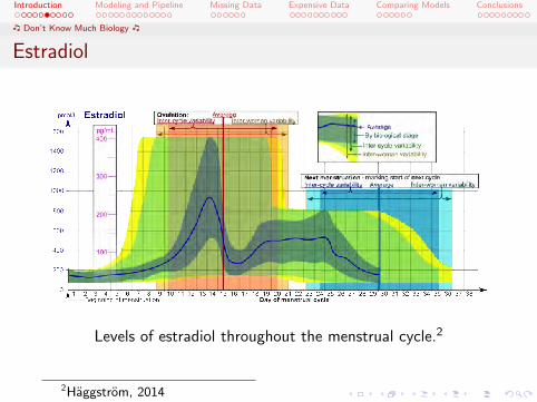
Estradiol
The other hormone we will consider is estrone 3-glucuronide(E13G), which is used as a marker for estradiol levels.
In the follicular phase, estradiol rises as the oocyte within afollicle matures into a viable egg. When estradiol levels risesufficiently, the hormone kicks off a chain of events that leadto the LH surge and ovulation.
In the luteal phase, estradiol (with progesterone) is critical tothe development of the endometrium, the lining of the uterusin which a fertilized egg would implant itself.
Introduction Modeling and Pipeline Missing Data Expensive Data Comparing Models Conclusions
� Don’t Know Much Biology �
Estradiol
Levels of estradiol throughout the menstrual cycle.2
2Haggstrom, 2014
Introduction Modeling and Pipeline Missing Data Expensive Data Comparing Models Conclusions
� Don’t Know Much Biology �
Polycyclic Aromatic Hydrocarbons – What They Are
Polycyclic aromatic hydrocarbons (PAHs) are organiccompounds containing only hydrogen and carbon in whichatoms are arranged in multiple connected rings.
PAHs can be considered a type of environmental pollutant.They are often produced through incomplete combustion oforganic matter (e.g. oil, coal, and tar).
We frequently encounter them through grilled meats, cigarettesmoke, engine exhaust, etc.
Introduction Modeling and Pipeline Missing Data Expensive Data Comparing Models Conclusions
� Don’t Know Much Biology �
Polycyclic Aromatic Hydrocarbons – What We Know
PAHs build up in the human body, and exposure levels can bemonitored by looking at PAH concentration in urine samplesand stool samples.
Epidemiologial studies have linked PAH exposure in utero withlow birth weight3, reduced immune function4, and impairedneurological development5.
Animal studies have shown that certain PAHs causesignificant follicular damage in female mice and rats6.
3Sram et al, 20054Winans et al, 20115Suades-Gonzalez et al, 20156Takizawa et al, 1984; Borman et al, 2000
Introduction Modeling and Pipeline Missing Data Expensive Data Comparing Models Conclusions
� Don’t Know Much Biology �
Polycyclic Aromatic Hydrocarbons – What We Use
Naphthalene
Fluorene
Phenanthrene
Pyrene
Introduction Modeling and Pipeline Missing Data Expensive Data Comparing Models Conclusions
� Don’t Know Much Biology �
Polycyclic Aromatic Hydrocarbons – Those Crazy Numbers
I’ll be talking about a lot of numbered PAH compounds, like2-hydroxyl naphthalene (2NAP) or 9-hydroxyl fluorene(9FLUO).
These are hydroxylated PAHs – PAHs that have had ahydroxyl group (-OH) added to them.
Hydroxylation is a detoxification process by which organismsbreak down organic compounds into compounds that are moreeasily excreted.
The numbering associated with these OH-PAHs refers to thebind point in the PAH where the hydroxyl group connects.
Introduction Modeling and Pipeline Missing Data Expensive Data Comparing Models Conclusions
Defining Our Objective
An Analysis Hierarchy
Data Exploration
_
Model Building
_
Model Validation
_
Prediction
Introduction Modeling and Pipeline Missing Data Expensive Data Comparing Models Conclusions
Defining Our Objective
Our Question of Interest
Research Question:
Do OH-PAHs have an effect on hormone levels and ovulationduring the human menstrual cycle?
Introduction Modeling and Pipeline Missing Data Expensive Data Comparing Models Conclusions
Defining Our Objective
Our Place in the Hierarchy
Data Exploration
_
Model Building
_
Model Validation
_
Prediction
Although previous work linkingPAH to fertility has been done inanimals, this is the first majorstudy examining the link inhumans.
We don’t really know what toexpect.
We want to establish whetherPAHs are important to this topicand begin looking at their role.
We’re not ready to validate amodel or predict outcomes.
Introduction Modeling and Pipeline Missing Data Expensive Data Comparing Models Conclusions
Key Modeling Concerns
Response Variables – General
Menstrual Cycle Length – What it says on the tin, this isjust how many days a woman’s menstrual cycle lasts. Weremove all cycles lasting longer than 35 days, which aregenerally anovulatory cycles and thus members of afundamentally different population than the ¡35 day cycles.
Follicular Phase Length – How many days pass betweenmenses and the LH surge. We need to detect an LH surge torecord this.
Ovulation Status – Whether ovulation occurred or not (asmeasured by whether we can detect an LH surge). This turnsout to be a complicated diagnostic testing problem because ofmissing data issues, and we won’t be considering it here.
Introduction Modeling and Pipeline Missing Data Expensive Data Comparing Models Conclusions
Key Modeling Concerns
Response Variables – LH-based
Average Follicular Phase LH Level – Recall that thehormone profile for LH during the menstrual cycle shows verylow baseline levels everywhere except at the LH surge. This isa measure of ground-state LH levels.
Highest Observed LH Level – When we believe a surgeoccurred, this is the highest LH level we recorded.
Peak Level at LH Surge – When we have complete data forthe days surrounding the surge, this is the level we observe atthe peak. (Peak LH and Highest LH are identical when bothare recorded; Peak LH has some missing values where HighestLH is recorded, though.
Introduction Modeling and Pipeline Missing Data Expensive Data Comparing Models Conclusions
Key Modeling Concerns
Response Variables – E13G-based
Average Follicular Phase E13G Level – This is the groundstate for estradiol observed early in the follicular phase.
Slope of Pre-Ovulatory E13G Rise – Recall that estradiolincreases as the follicles mature during the cycle, and thenafter a certain threshold is reached, this begins a chainreaction resulting in the LH surge. E13G Slope is the rate ofincrease in estradiol during this process.
Peri-ovulatiory E13G Level – Recall also that estradiol dropsoff again during the LH surge. This is a measure of estradiollevels at that time.
Introduction Modeling and Pipeline Missing Data Expensive Data Comparing Models Conclusions
Key Modeling Concerns
Predictors of Interest
We have a large group ofpredictors we can draw fromin this problem.
However, we’re onlyinterested in whether PAHshave an effect on hormonelevels.
We want to make the mosteffective use of ourpredictors in answering ourkey question.
Baseline covariates:
Race Stress EducationAge Caffeine IntakeBMI Alcohol ConsumptionWalking Minutes per WeekVigorous Activity per Week
PAH covariates:
2Fluo 3Fluo 9Fluo1Phen 2Phen 3Phen1Nap 2Nap 1Pyr
Introduction Modeling and Pipeline Missing Data Expensive Data Comparing Models Conclusions
Key Modeling Concerns
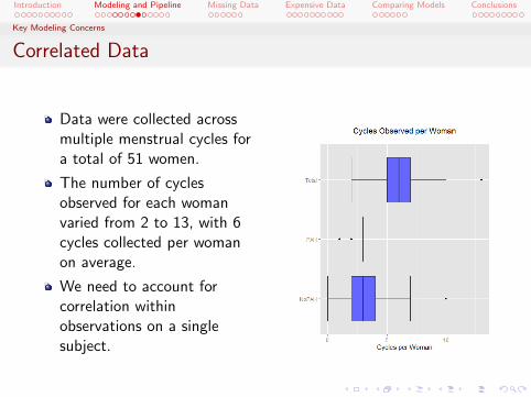
Correlated Data
Data were collected acrossmultiple menstrual cycles fora total of 51 women.
The number of cyclesobserved for each womanvaried from 2 to 13, with 6cycles collected per womanon average.
We need to account forcorrelation withinobservations on a singlesubject.
Introduction Modeling and Pipeline Missing Data Expensive Data Comparing Models Conclusions
Key Modeling Concerns
Bayesian vs. Frequentist
With complicated modeling situations, the Bayesian approachis often easier to construct and understand.
Construction – the missing data situations in our problemmake a Bayesian approach much more tractable here.
Understanding – as you’ll see in a second, the model we comeup with is pretty complicated. It’s a lot easier to keep track ofthe various parts of that model, and to make sure we’remaking reasonable assumptions about those parts, when weput everything into a Bayesian framework.
Introduction Modeling and Pipeline Missing Data Expensive Data Comparing Models Conclusions
The Setup
The Analysis Pipeline
Recall that our primary interest is in detecting whetherOH-PAHs have an effect on our response variables.
More than that, we’re interested in whether they have ameaningful effect—that is, do OH-PAHs tell us somethingabout our response variables that we can’t learn more easilywith other predictors?
We will consider two models for each endpoint:
1. A baseline model using only our non-PAH predictors.2. A final model using both non-PAH predictors and our OH-PAH
concentrations.
We will compare these two models to see which one is better.
Introduction Modeling and Pipeline Missing Data Expensive Data Comparing Models Conclusions
The Setup
The Model Structure
We begin with the basic linear mixed model:
Yij = Xijβ + Zijγi + εij .
In an easy setting, we’d assume something like:
εijiid∼ N(0, σ2), γi
iid∼ N(0, τ2).
We’ll have to do things a little differently to deal with missingdata—specifically, our εij ’s aren’t going to be identicallydistributed.
Introduction Modeling and Pipeline Missing Data Expensive Data Comparing Models Conclusions
The Setup
How We Get Our Models
We will use a backward stepwise procedure to get our models.
For the baseline model:
1. We use MCMC to fit a model with all non-PAH predictorsincluded.
2. For each β in the model, we calculate the proportion ofiterates that were above zero. Call this pβ .
3. We drop the covariate for which pβ is closest to 50%. If thecovariate is a factor variable, we consider only the pβ farthestfrom 0.5 among the β’s for all its levels.
4. We refit the model until all remaining covariates havepβ > 0.85 or pβ < 0.15 (i.e. until all remaining coefficients areconsistently positive or negative).
5. Covariates for Age and Race are forced into the model becausewe believe a priori that they are important to modeling ourresponse variables.
Introduction Modeling and Pipeline Missing Data Expensive Data Comparing Models Conclusions
The Setup
How We Get Our Models
We will use a backward stepwise procedure to get our models.
For the model including OH-PAH covariates:
1. Our initial model includes all the non-PAH predictors from thebaseline model, as well as all the OH-PAH predictors.
2. We conduct the same stepwise procedure using pβ , removingwhichever covariate has pβ closest to 50%.
3. Again, we refit the model after each covariate is removed untilall remaining covariates have pβ > 0.85 or pβ < 0.15.
4. We do allow the model to drop non-PAH covariates if theirpβ ’s fall back below the retention threshold after OH-PAHcovariates are included.
Introduction Modeling and Pipeline Missing Data Expensive Data Comparing Models Conclusions
The Problem
Traditional Missing Data – Predictors
Our study has a lot of self-report data on demographicpredictors that we’re interested in using.
Unsurprisingly, though, when you give a lot of surveys to a lotof people, some of them won’t complete every survey, or willprovide data that isn’t easy to categorize.
For BMI, Stress, Education, Caffeine Intake, and AlcoholConsumption, we are missing data for 1-3 women (out of atotal sample of k = 51).
We will assume these data are missing at random – that thereare no systematic differences between the women for whomthese data are missing and the women for whom these dataare present.
Thankfully, we have very little missing predictor data, so ouranalysis is probably robust to this assumption.
Introduction Modeling and Pipeline Missing Data Expensive Data Comparing Models Conclusions
The Problem
Traditional Missing Data – Responses
The missing data problem on our response variables is trickier.
Most of the responses we’re using are calculated from raw,daily data obtained by an electronic device that monitorshormone concentrations in urine. Again unsurprisingly, peoplediffer in their commitment to peeing on a stick every morningin the pursuit of science.
It is probably unreasonable to assume that there are noimportant differences between women for whom we have moreconsistent data and women for whom we lack consistentdata...
But we can still make the MAR assumption—that conditionalon what we know about these women through our model,there is no systematic differences between cycles where wehave consistent data and cycles where we don’t.
Introduction Modeling and Pipeline Missing Data Expensive Data Comparing Models Conclusions
Our Solution
Simple Bayesian Imputation
Missing data is a common complication in data analysis, butthe Bayesian approach makes dealing with it very easy.
On the next two slides, I’ll give two examples of WinBUGScode. The first is a complete data formulation; the second is amissing data formulation.
The change here is relatively minor—though it will have someknock-on effects on our ability to compare models down theroad.
Introduction Modeling and Pipeline Missing Data Expensive Data Comparing Models Conclusions
Our Solution
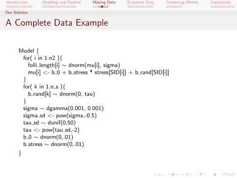
A Complete Data Example
Model {for( i in 1:n2 ){
folli length[i] ∼ dnorm(mu[i], sigma)mu[i] <- b 0 + b stress * stress[SID[i]] + b rand[SID[i]]}for( k in 1:n s ){
Introduction Modeling and Pipeline Missing Data Expensive Data Comparing Models Conclusions
Our Solution
In the BUGS setting, all we have to do is add statements toindicate that our covariate will be probabilistically modeledwith some given prior distribution.
Whenever data are available, the MCMC will use the actualdata for the variable.
When data aren’t available, the MCMC will impute thevariable automatically, given its role in the model.
In the example above, if information on Stress is missing, theMCMC will tend toward a weighted average of a brand termand a stress term according to their respective variances andthe stress coefficient.
If we think about what this means in terms of the model,that’s exactly what we want.
Introduction Modeling and Pipeline Missing Data Expensive Data Comparing Models Conclusions
The Problem
OH-PAH Data Costs Money
We’ve got a different type of missing data situation going onwith our OH-PAH predictors.
OH-PAH data are collected once per cycle for each woman,on the 10th day after menses.
OH-PAH concentrations are measured from a urine sample(collected independently of daily hormone measurements).
We pay the CA Dept. of Public Health’s EnvironmentalHealth Lab to calculate the OH-PAH concentrations based onthe urine samples we’ve collected.
Unfortunately, we run out of money to pay the lab before werun out of samples to test.
Introduction Modeling and Pipeline Missing Data Expensive Data Comparing Models Conclusions
The Problem
What We Can Access
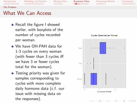
Recall the figure I showedearlier, with boxplots of thenumber of cycles recordedper woman.
We have OH-PAH data for1-3 cycles on every woman(with fewer than 3 cycles iffwe have 3 or fewer cyclestotal for the woman).
Testing priority was given forsamples corresponding tocycles with more completedaily hormone data (c.f. ourissue with missing data onthe responses).
Introduction Modeling and Pipeline Missing Data Expensive Data Comparing Models Conclusions
The Problem
How Does OH-PAH Missingness Affect Our Analysis
As always, we should worry about the MCAR/MAR/MNARassumptions. We have a process to choose which samples totest. Are samples we test likely to be structurally differentfrom samples we don’t test, conditional on the otherinformation we have?
It is likely that missingness in response data is related toindividual subjects – and this is important because it’s part ofour algorithm for choosing which OH-PAH samples to test.
It is unlikely that missingness is related to individual cycles,conditional on subject.
Since we are making sure to get 3 OH-PAH samples fromevery subject based on the cycles with her most completeresponse data, we should be able to make the MARassumption.
Introduction Modeling and Pipeline Missing Data Expensive Data Comparing Models Conclusions
The Problem
How Does OH-PAH Missingness Affect Our Analysis
We have another serious problem here, though. Rememberthat the whole point of our study is to identify whetherOH-PAH’s have an effect on hormones levels during, andcharacteristics of, the menstrual cycle.
We only have data on OH-PAH concentrations for a bit underhalf (48%) of cycles we studied.
Do we have to throw out half of our data because it doesn’ttalk about our research question, or is there something else wecan do?
Introduction Modeling and Pipeline Missing Data Expensive Data Comparing Models Conclusions
Our Solution
Shared-Parameter Modeling
Think about the role our classes of variables play here:
Response – For which we want to build a model.
OH-PAH Predictor – For which we want to determine whetherthey have a role in that model.
Non-PAH Predictor – For which we want to control, so wecan see whether the OH-PAH predictors’ role is practicallymeaningful.
Introduction Modeling and Pipeline Missing Data Expensive Data Comparing Models Conclusions
Our Solution
Shared-Parameter Modeling
We would like to use the information on the PAH-missingdata to help us understand the role the non-PAH covariatesplay in the model.
We can do this by assuming that we’re modeling the sameparameters when we have PAHs and when we don’t havePAHs.
Let’s take a look at what this means in terms of WinBUGScode:
Introduction Modeling and Pipeline Missing Data Expensive Data Comparing Models Conclusions
Our Solution
The PAH-Missing Model
Model {for( i in 1:n2 ){
folli length[i] ∼ dnorm(mu[i], sigma)mu[i] <- b 0 + b stress * stress[SID[i]] + b rand[SID[i]]}for( k in 1:n s ){
b rand[k] ∼ dnorm(0, tau)stress[k] ∼ dnorm(mu stress,sigma stress)}...
}
Introduction Modeling and Pipeline Missing Data Expensive Data Comparing Models Conclusions
Our Solution
The PAH-Included Model
Model {for( i in 1:n1 ){
folli length[i] ∼ dnorm(mu[i], sigma 1 )mu[i] <- b 0 + b stress * stress[SID[i]] + b rand[SID[i]]}for( i in (n1+1):n2 ){folli length[i] ∼ dnorm(mu[i], sigma 2)mu[i] <- b 0 + b stress * stress[SID[i]] + b rand[SID[i]] +
b pah[1] * Cr 1PYR[i] + b pah[2] * Cr 3FLUO}for( k in 1:n s ){
b rand[k] ∼ dnorm(0, tau)stress[k] ∼ dnorm(mu stress,sigma stress)}...
}
Introduction Modeling and Pipeline Missing Data Expensive Data Comparing Models Conclusions
Our Solution
What Are We Doing?
We fit a model without OH-PAHs on the PAH-missing data,and then we fit a second model on the PAH-included data.
These two models share parameters for the intercept and foreach non-PAH covariate.
These two models also share random effects terms, becausethe random effect value is subject-specific and subjects haveobservations in both models.
The error variance on the models is different, because weexpect that we are accounting for more response variability inthe PAH-included data.
Introduction Modeling and Pipeline Missing Data Expensive Data Comparing Models Conclusions
Our Solution
Places to Be Cautious
By structuring these two models with shared parameters, weassume that these parameters will be the same across models.
This is stricter than simply assuming the parameters should berelated between models, and involves a complicated set ofassumptions.
In particular, I worry about:
Whether the OH-PAH covariates have a biasing effect. Wedeal with this by standardizing the OH-PAH values so theyhave mean 0. (I think) we could also let the intercept term inthe two models differ.Whether there is collinearity between OH-PAH concentrationsand the non-PAH covariates. There is, which means that ourestimates of the non-PAH parameters in the PAH-includedmodel will probably shrink towards zero, relative to ourestimates from the PAH-missing model.
Introduction Modeling and Pipeline Missing Data Expensive Data Comparing Models Conclusions
The Problem
How We Select Our Models
Recall that we obtain our models through a pair of backwardstepwise procedures.
We choose to remove and retain covariates based on pβ, ameasure of the proportion of iterates from the posteriordistribution for β that fall below 0.
Selection by pβ is ad-hoc, and while it seems reasonable forthe stepwise procedure where we’re using it, we would preferto have additional criteria for evaluating the relative quality ofour models.
Introduction Modeling and Pipeline Missing Data Expensive Data Comparing Models Conclusions
The Problem
Traditional Model Selection Criteria
If we weren’t being Bayesians, we might choose something likeAIC with its ties to the Kullback-Leibler divergence.
As Bayesians, though, we have three traditional measures offit we might consider:
Bayes Factor (BF) – Analogous to a likelihood ratio; looks atthe ratio of the probability of the data arising under the twomodels being compared.Log Pseudo-marginal Likelihood (LPML) – Like the BayesFactor, but involves looking at how well the model fits thedata when that data point is not used in fitting the model;analogous to a leave-one-out approach to the BF.Deviance Information Criterion (DIC) – Computationally“easy”, a weighted measure of the difference between themean posterior (Bayesian) deviance under a model, and the(Bayesian) deviance evaluated at the posterior mean.
Introduction Modeling and Pipeline Missing Data Expensive Data Comparing Models Conclusions
The Problem
Different Types of DIC
In the original development of DIC7, the authors discuss theidea of focal parameters and suggest marginalizing outnon-focal parameters before computing the DIC.
This is difficult to do in practice. The great advantage of DICis its computability—but its computability relies on having thejoint distribution of all parameters in the model.
In the random effects and missing data settings, variants ofthe traditional DIC have been proposed8 to deal withmismatch between the focal parameters and the parametersactually modeled.
7Spiegelhalter et al, 20028Celeux et al, 2006
Introduction Modeling and Pipeline Missing Data Expensive Data Comparing Models Conclusions
The Problem
What WinBUGS Provides
WinBUGS calculates a DIC score automatically.
“This deviance is defined as -2 * log(likelihood): ’likelihood’ isdefined as p(y |θ), where y comprises all stochastic nodes givenvalues (i.e. data), and θ comprises the stochastic parents of y –’stochastic parents’ are the stochastic nodes upon which thedistribution of y depends, when collapsing over all logicalrelationships.”
Unfortunately, this is not the deviance we want. It treats boththe random effects and the parameters used to model ourmissing covariates as focal parameters.
Introduction Modeling and Pipeline Missing Data Expensive Data Comparing Models Conclusions
Our Solution
The Marginal DIC
We can get D(θ|Y ) directly in this problem, by using themultivariate normal distribution with covariance matrixcorresponding to the random effects model.
We ignore the effect of missing data on the DIC, because themissing data relates to the observed data but not the modelparameters themselves.
The current solution is computationally intensive (it takesabout 10m to calculate the DIC for each model), but it istractable, and it gives us the correct DIC.
Introduction Modeling and Pipeline Missing Data Expensive Data Comparing Models Conclusions
Some Interesting Results
Areas Where PAHs Seem Important
Basically everywhere.
We show a DIC reduction of 3 or more9 in our models forcycle length, follicular phase length, follicular LH level, highestobserved LH level, peak LH level, and slope of pre-ovulatoryestradiol rise.
Only models for follicular estradiol level and periovulatoryestradiol level don’t appear to show significant improvementwith the inclusion of OH-PAH concentrations.
9A difference 3 is suggested by Spiegelhalter et al (2002) as sufficientindication that one model is preferred to another.
Introduction Modeling and Pipeline Missing Data Expensive Data Comparing Models Conclusions
Some Interesting Results
Which PAHs Seem Important
Pyrene plays a role in cycle length, follicular phase length, andfollicular phase LH levels.
Fluorene is indicated in models for cycle length, follicularphase length, and surge LH levels.
Naphthalene appears in all LH models, as well as E13G Slope.
Phenanthrene appears in models for all response variablesexcept follicular phase length.
Introduction Modeling and Pipeline Missing Data Expensive Data Comparing Models Conclusions
Some Interesting Results
The Role of PAH Profiles
OH-PAH concentrations tend to be highly collinear, especiallyamong different isomers of the same compound.
Naphthalene is an exception to this – 1- and 2-naphthaleneare known to arise from exposure to different pollutants.
Because of collinearity, we model fluorene and phenanthrenewith both an “average concentration” term and terms for thedegree to which individual isomers deviate from the average.
We find that the profile of isomers being created appears justas influential as the overall concentration of the OH-PAHs.
Introduction Modeling and Pipeline Missing Data Expensive Data Comparing Models Conclusions
Some Interesting Results
From the Data Analysis
Plots of 1-naphthalene vs. highest observed LH for variousconcentrations of fluorene isomers.
Introduction Modeling and Pipeline Missing Data Expensive Data Comparing Models Conclusions
� Where Do We Go from Here? �
Revisiting the Analysis Hierarchy
Data Exploration
_
Model Building
_
Model Validation
_
Prediction
We’ve verified that PAHconcentrations are predictive ofhormone levels during the humanmenstrual cycle.
We’ve begun to examine possiblemodels of their action.
Further research should considerbiologic pathways through whichthey may act, and should seek toverify and expand upon the resultswe’ve found.
Introduction Modeling and Pipeline Missing Data Expensive Data Comparing Models Conclusions
� Where Do We Go from Here? �
The Ovulation Model Problem
I mentioned early on that we wanted to look at whetherovulation occurred as a response variable. It’s actually theresponse variable we’re most interested in studying with thesedata.
Unfortunately, the missing data issues described abovebecome even more complicated for ovulation, because MAR isno longer a valid assumption.
The problem we encounter is that our proxy for whetherovulation occurred is our detection of an LH surge. If we see asurge, we say ovulation occurred.
If we don’t see a surge, it may be because no surge occurred,or because we don’t have data for the 2-3 days during whichwe would observe heightened LH levels.
Introduction Modeling and Pipeline Missing Data Expensive Data Comparing Models Conclusions
� Where Do We Go from Here? �
The Ovulation Model Problem
What we end up with is a division of observations into threecategories:
(A) Observations where we know an LH surge occurred (i.e. wesaw a surge).
(B) Observations where we know no LH surge occurred (i.e. wehave complete data and can see nothing happened).
(C) Observations where we’re unsure whether a surge occurred.
The problem here is that our criteria for sorting observationsinto groups (A) and (B) aren’t equally stringent. We aremuch more likely to see a surge than to see enoughobservations to be certain no surge occurred.
Because our missingness mechanism is directly tied to whatwe want to predict, we need a different approach (e.g. thediagnostic testing paradigm).
Introduction Modeling and Pipeline Missing Data Expensive Data Comparing Models Conclusions
We’re almost done!
Bibliography
SM Borman, PJ Christian, IG Sipes, & PB Hoyer. (2000) “Ovotoxicity infemale Fischer rats and B6 mice induced by low-dose exposure to threepolycyclic aromatic hydrocarbons: Comparison through calculation of anovotoxic index.” Toxicology and Applied Pharmacology 167 191-198.
G Celeux, F Forbes, CP Robert, & DM Titterington. (2006) “Devianceinformation criteria for missing data models.” Bayesian Analysis 1,651-674.
M Haggstrom. (2014) “Reference ranges for estradiol, progesterone,luteinizing hormone and follicle-stimulating hormone during the menstrualcycle.” Wikiversity Journal of Medicine 1 (1).
RJ Sram, B Binkova, J Dejmek, & M Bobak. (2005) “Ambient airpollution and pregnancy outcomes: a review of the literature.”Environmental Health Perspectives 113, 375-382.
Introduction Modeling and Pipeline Missing Data Expensive Data Comparing Models Conclusions
We’re almost done!
Bibliography
E Suades-Gonzalez, M Gascon, M Guxens, & J Sunyer. (2015) “Airpollution and neuropsychological development: a review of the latestevidence.” Endocrinology 156, 3473-3482.
DJ Spiegelhalter, NG Best, BP Carlin, & A van der Linde. (2002)“Bayesian measures of model complexity and fit.” J.R. Statist. Soc. B64, 583-639.
K Takizawa, H Yagi, DM Jerina, & DR Mattison. (1984) “Murine straindifferences in ovotoxicity following intraovarian injection withbenzo(a)pyrene, (+)-(7R,8S)-oxide, (-)-(7R,8R)-dihydrodiol, or”(+)-(7R,8S)-diol-(9S,10R)-epoxide-2.” Cancer Research 44, 2571-2576.
B Winans, MC Humble, & BP Lawrence. (2011) “Environmentaltoxicants and the developing immune system: A missing link in the globalbattle against infectious disease?” Reproductive Toxicology 31, 327336.