A Bayesian Framework for Statistical Signal Processing and Knowledge Discovery in Proteomic Engineering

by

Gil Alterovitz

B.S., Electrical and Computer Engineering Carnegie Mellon University, 1998

S.M., Electrical Engineering and Computer Science

Massachusetts Institute of Technology, 2001

SUBMITTED TO THE HARVARD-MIT DIVISION OF HEALTH SCIENCES AND TECHNOLOGY IN PARTIAL FULFILLMENT OF THE REQUIREMENTS FOR THE

DEGREE OF

DOCTOR OF PHILOSOPHY IN ELECTRICAL AND BIOMEDICAL ENGINEERING AT THE

MASSACHUSETTS INSTITUTE OF TECHNOLOGY

June 2005

© 2005 Massachusetts Institute of Technology. All rights reserved.

Signature of Author………………………………………………………………………………………………

Harvard-MIT Division of Health Sciences and Technology June 1, 2005

Certified by……………………………………………………………………………………………………

Marco F. Ramoni, Ph.D. Assistant Professor

Harvard-MIT Division of Health Sciences and Technology Thesis Supervisor

Certified by……………………………………………………………………………………………………

Isaac S. Kohane, M.D., Ph.D. Lawerence J. Henderson Associate Professor

Harvard-MIT Division of Health Sciences and Technology Thesis Supervisor

Accepted by……………………………………………………………………………………………………

Martha L. Gray, Ph.D. Edward Hood Taplin Professor of Medical and Electrical Engineering

Co-Director, Harvard-MIT Division of Health Sciences and Technology

2

Dedicated to Samuel, Dalia, and Ron Alterovitz …

3

Table of Contents ABSTRACT .................................................................................................................................................................5

CHAPTER I: OVERVIEW.................................................................................................................................6 I.A. INTRODUCTION ......................................................... 6 I.B. OUTLINE ............................................................. 7

CHAPTER II: BACKGROUND ..........................................................................................................................9 II.A. PROTEOMICS OVERVIEW .................................................. 9 II.B. TECHNOLOGIES & AUTOMATION IN PROTEOMICS................................. 15 II.C. STATISTICAL AND MACHINE LEARNING METHODS................................ 33

CHAPTER III: BAYESIAN APPROACH .........................................................................................................34 III.A. GRAPHICAL MODELS ................................................... 34 III.B. BUILDING A BAYESIAN FOUNDATION ........................................ 35 III.C. FRAMEWORK ......................................................... 39

CHAPTER IV: BAYESIAN PROTEIN IDENTIFICATION...........................................................................41 IV.A. DISEASE PROFILE ANALYSIS............................................. 41 IV.B. STATISTICAL SIGNAL PROCESSING......................................... 51 IV.C. PROTEIN IDENTIFICATION VIA MASSOME OF PROTEIN INTERACTIONS ................. 62

CHAPTER V: CONCLUSION AND DISCUSSION .......................................................................................68 V.A. SUMMARY AND CONTRIBUTIONS .............................................. 68 V.B. IMPLICATIONS AND LIMITATIONS ........................................... 70 V.C. FUTURE WORK AND CONCLUSION ............................................. 71

CHAPTER VI: REFERENCES...........................................................................................................................73

CHAPTER VII: ACKNOWLEDGEMENTS......................................................................................................86

CHAPTER VIII: APPENDIX ..............................................................................................................................88 VIII.A. MATHEMATICAL NOTATION.............................................. 88 VIII.B. GLOSSARY ........................................................ 89

4

List of Figures FIGURE 1: NUMBER OF ENTRIES IN ENTREZ NUCLEOTIDE AND PROTEIN DATABASES ..............................................11 FIGURE 2: AUTOMATION, ROBOTICS, AND BIOMEDICAL ENGINEERING-RELATED PAPERS ARE GROWING AT A MUCH

FASTER RATE THAN THE PAPERS IN ALL FIELDS IN THE PUBMED DATABASE. ....................................................16 FIGURE 3: MASS SPECTROMETRY IS GROWING AT A MUCH FASTER RATE IN TERMS OF PAPERS COMPARED TO THE

GENERAL PUBMED DATABASE. ...........................................................................................................................21 FIGURE 4: SELDI-TOF MASS SPECTROMETRY SCHEMATIC ......................................................................................25 FIGURE 5. STEPS INVOLVED IN PRE-FILTERING AND TANDEM MASS SPECTROMETRY ...............................................26 FIGURE 6: CONDITIONAL PROBABILITY TABLES (CPT)................................................................................................37 FIGURE 7: NAÏVE BAYESIAN CLASSIFIER: DIRECTED GRAPH WITH CONDITIONAL INDEPENDENCE ASSUMPTION ..........38 FIGURE 8: CANONICAL BAYESIAN NETWORK 2: DIRECTED GRAPH WITH MARGINAL INDEPENDENCE ASSUMPTION ......38 FIGURE 9: HIERARCHICAL LEVELS OF ANALYSIS FOR THE BAYESIAN FRAMEWORK .....................................................40 FIGURE 10: SELDI MASS SPECTROMETRY DATA AXES .................................................................................................42 FIGURE 11: A SIMPLE BAYESIAN CLASSIFIER ...............................................................................................................43 FIGURE 12: PERFORMANCE ON DIFFERENT METRICS.....................................................................................................45 FIGURE 13: 8602.384 NODE NEIGHBORHOOD DEPENDENCIES .......................................................................................47 FIGURE 14: CONSTRUCTING A BAYESIAN NETWORK FROM PRELEUKEMIA PROTEOMIC DATA ......................................50 FIGURE 15: CONSTRUCTING A BAYESIAN NETWORK FROM OVARIAN CANCER PROTEOMIC DATA.................................51 FIGURE 16: OVERVIEW OF PROTEIN IDENTIFICATION ANALYSIS METHODOLOGY..........................................................52 FIGURE 17: MARKOV BLANKET OF SELECTED NODE (CIRCLED)....................................................................................54 FIGURE 18: ESTIMATION OF STANDARD DEVIATION PARAMETER VIA FULL WIDTH AT HALF MAXIMUM (FWHM)........56 FIGURE 19: MAPPING MASS SPECTROMETRY PEAKS TO PROTEIN IDENTIFICATIONS VIA NETWORK MAPPING................57 FIGURE 20: (A) PEAK FROM HIGH-RESOLUTION DATASET IN LOCAL PEAK ENVIRONMENT, (B) ISOLATED PEAK...........58 FIGURE 21: ESTIMATION FOR ΣM/Z (PLUS ERROR BARS)..................................................................................................58 FIGURE 22: ALL POTENTIAL ESTIMATED BIOMARKER PEAKS........................................................................................59 FIGURE 23: ONE ESTIMATED BIOMARKER PEAK............................................................................................................60 FIGURE 24: MARKOV BLANKET FOR 7755.61 M/Z NODE ...............................................................................................61 FIGURE 25: SUBNETWORK FROM PROTEOMIC TEST DATASET .......................................................................................62 FIGURE 26: SCHEMATIC OF AUTOMATED MASSOME DATABASE CREATION...................................................................64 FIGURE 27: SCHEMATIC OF MASSOME DATABASE USAGE FOR PROTEIN IDENTIFICATION..............................................65 FIGURE 28: 3-D VISUALIZATION OF A PORTION OF THE HUMAN MASSOME OF PROTEIN INTERACTIONS ........................66 FIGURE 29: VALIDATION OF INTERACTION PREDICTIVE ABILITY IN PRELEUKEMIA DATASET........................................67 FIGURE 30: PREDICTION EXAMPLE FOR OVARIAN CANCER DATASET ............................................................................67

5

A BAYESIAN FRAMEWORK FOR STATISTICAL SIGNAL PROCESSING AND KNOWLEDGE DISCOVERY IN PROTEOMIC ENGINEERING

By

GIL ALTEROVITZ

Submitted to the Harvard-MIT Division of Health Sciences and Technology on June 1, 2005 in partial fulfillment of the requirements for the Degree of Doctor of Philosophy

in Electrical and Biomedical Engineering

ABSTRACT

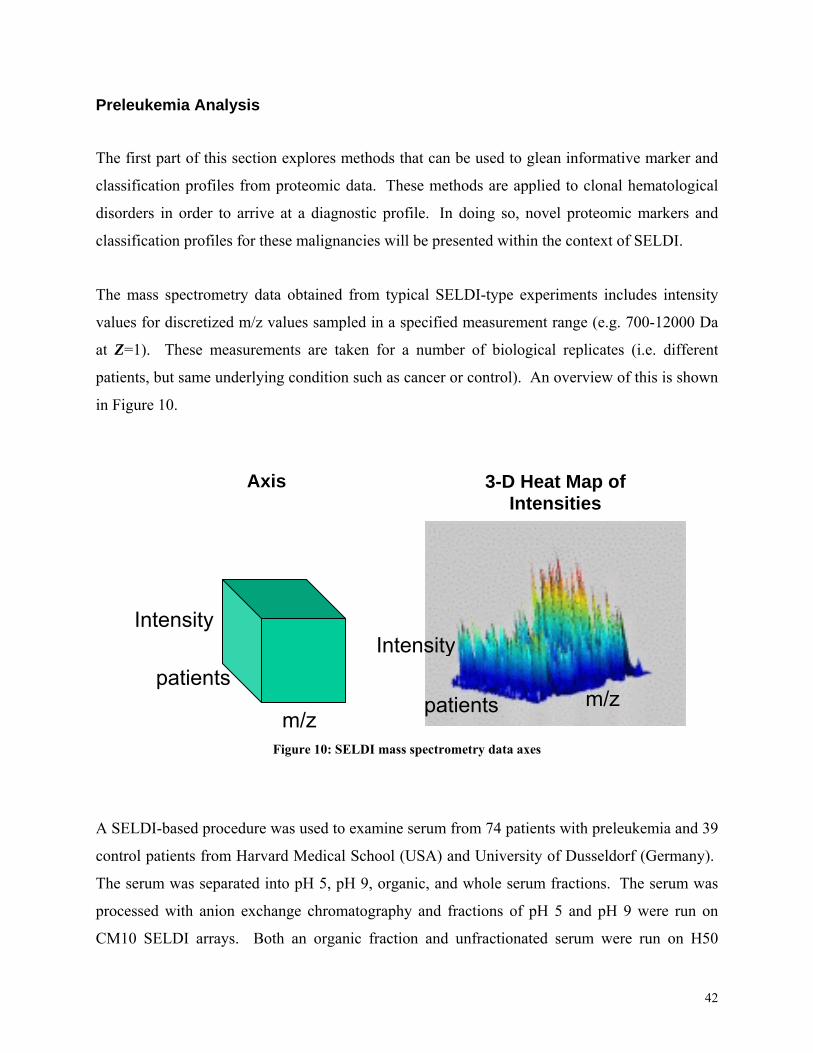
Proteomics has been revolutionized in the last couple of years through integration of new mass spectrometry technologies such as Surface-Enhanced Laser Desorption/Ionization (SELDI) mass spectrometry. As data is generated in an increasingly rapid and automated manner, novel and application-specific computational methods will be needed to deal with all of this information. This work seeks to develop a Bayesian framework in mass-based proteomics for protein identification. Using the Bayesian framework in a statistical signal processing manner, mass spectrometry data is filtered and analyzed in order to estimate protein identity. This is done by a multi-stage process which compares probabilistic networks generated from mass spectrometry-based data with a mass-based network of protein interactions. In addition, such models can provide insight on features of existing models by identifying relevant proteins. This work finds that the search space of potential proteins can be reduced such that simple antibody-based tests can be used to validate protein identity. This is done with real proteins as a proof of concept. Regarding protein interaction networks, the largest human protein interaction meta-database was created as part of this project, containing over 162,000 interactions. A further contribution is the implementation of the massome network database of mass-based interactions- which is used in the protein identification process. This network is explored in terms potential usefulness for protein identification. The framework provides an approach to a number of core issues in proteomics. Besides providing these tools, it yields a novel way to approach statistical signal processing problems in this domain in a way that can be adapted as proteomics-based technologies mature. Thesis Supervisor: Marco F. Ramoni, Ph.D. Title: Assistant Professor, Harvard-MIT Division of Health Sciences and Technology Thesis Supervisor: Isaac S. Kohane, M.D., Ph.D. Title: Lawerence J. Henderson Associate Professor, Harvard-MIT Division of Health Sciences and Technology

6

CHAPTER I: OVERVIEW

I.A. Introduction

With the completion of the human genome project, the genetic sequence of humans has been

effectively determined. Yet, the source of the complexity of humans relative to other organisms

has not been fully elucidated: consider that the number of genes in C. elegans (worm) is on the

same order of magnitude as that of humans: 2x104 [1]. It has been conjectured that this situation

can be explained by a layer of protein-protein interactions, responsible for the expected

difference in functional richness between worms and humans- since as the number of proteins n

increases, the potential interactions increases as Θ(n2) (proportional to n2).

Through improved technologies such as automated sequencing, microarrays, and mass

spectrometry, all three levels of the central dogma of molecular biology [2] (i.e. DNA, RNA,

protein) are being explored on an organism-level scale. Genomics looks at gene-based

information by mapping DNA of organisms. The genome refers to the complete sequence map

of an organism. The transcriptome represents mRNA/expression-based information.

Completing the triad is the proteome, the set of all proteins in an organism (or subcomponent).

Proteomics studies these proteins and the links between them on a large scale.

Proteomics has been revolutionized in the last couple of years through integration of new mass

spectrometry technologies such as SELDI mass spectrometry [3, 4]. SELDI can be used to

measure proteins in biological samples. One difference from current gene expression microarray

studies, where the genes are known, is that the identity of the proteins is usually unknown in

SELDI-based experiments. Thus, SELDI studies are struggling with actual protein

identification, often providing no more than a pattern-based predictor model.

A number of recent studies have looked at differential profiles as a way of classifying binary or

m-ary pathological states. Machine learning techniques have been employed for proteomic

profiling with clinically promising results [5-7]. Though these profiles are exciting in terms of

promising predictors, many of the current profiles are not practical and scientifically rewarding

7

since they rely on hundreds or thousands of protein peaks (most of which are unidentified).

Rather than identifying specific proteins, such studies have provided diagnostic information

solely based on “black box” predictors that look at differential patterns of mass spectrometry

peaks. Purification, isolation, and manual identification of just one peak-based protein can take

months.

As data are generated in an increasingly rapid and automated manner, novel and application-

specific computational methods will be needed to deal with all this information. Through use of

computational machine learning techniques described in this thesis (as well as the author’s work

described previously [8]), it is hoped that new protein predictors can be found that are clinically

practical and biologically plausible.

I.B. Outline

This work explores computational approaches by establishing a Bayesian framework. Various

incarnations of Bayesian approaches and related networks have been used recently in

bioinformatics from single nucleotide polymorphisms (SNPs) [9] (to learn about subtle

sequence-based relationships) to microarray data analysis (to learn transcription factors,

expression, and regulation pathways) [10, 11]. Here, a novel application and corresponding

methodology is explored.

Hypothesis: Protein network perturbations are relayed throughout constituent links in a

manner that identifies the underlying nodes and their relationships.

Traditionally, it has been believed that the protein masses in SELDI-type experiments cannot be

deconvolved/reconstructed and that proteins cannot be identified based on SELDI mass

spectrometry data [12]. The hypothesis in this thesis is that probabilistic relationships derived

from such mass spectrometry experiments can be used to estimate masses (from mass-to-charge

ratios), protein identities, and other information about pathology. This approach is based on the

idea that perturbations to the network/system are relayed throughout the links in a manner

8

consistent with the topologic properties of the network. This notion of network-based

identification (applied to proteins) is delineated in section IV.C.

Objective: Use probabilistic relationships and topologic properties derived from mass

spectra biomarkers to create a unified Bayesian framework for predicting pathological

states and identifying relevant protein identities.

This research examines the use of Bayesian network structural learning to yield conditional

dependencies which implicitly encode important protein relationships. These networks can be

used to learn the relationships and interactions of these proteins by comparing the probabilistic

dependencies with a specialized database of protein interactions. This research examines issues

ranging from the meaning of probabilistic links between proteins in mass spectrometry to actual

protein identification from this information.

This objective is approached with three goals in mind:

Aim #1: Use probabilistic relationships encoded in mass spectra to predict pathology using

biomarker information.

In this work, we use this approach on two clinical diseases: preleukemia and ovarian cancer.

Insights are gained from the Bayesian analysis of mass spectra. Also, peaks beyond the

precision of the actual SELDI instrumentation can be discovered with this method. This

Bayesian network methodology, combined with the class/functional information that it suggests,

can help to predict the protein peaks with a one-to-many peak-to-protein mappings as well as the

many-to-one peak-to-protein correspondences. In doing so, better models for predicting disease

states can be created.

Aim #2: Develop and implement the concept of a ‘massome’ for facilitating mass

spectrometry-based protein identification.

9

A massome can be conceptualized as all of the masses present in an organism or subcomponent

(such as a tissue or organelle). Such masses can include a variety of biological molecules- from

proteins to metabolic pathway constituents. Each mass can be linked to its innate properties and

relationships- such as interactions encoded in a network. In this work, an instantiation of a

subset of this concept, namely the human massome of protein interactions, is used for protein

identification.

Aim #3: Predict protein identity by mapping probabilistic relationships encoded in mass

spectra to the human massome of protein interactions. Confirm model validity with real

pathology/biological findings.

The goal here is to show that by isolating probabilistically linked nodes and using additional

mass information (via massome database of protein interactions), the search space for protein

identification can be reduced and validation can be simplified in terms of both time and cost (e.g.

via simple antibody method). This work goes beyond delineating methods for disease analysis

and protein identification. It tests them via biological validation. In doing so, the results of the

methodology can be seen within the context of real world issues such as noise within

experimental mass spectrometry results.

CHAPTER II: BACKGROUND

II.A. Proteomics Overview

According to the central dogma of molecular biology [2], the blueprint for life is contained in a

string of nucleotides (chosen from an code set of four bases: adenosine, guanosine, thymidine

and cytidine) that form Deoxyribonucleic Acid (DNA). Through transcription, messenger

ribonucleic acid (RNA) is formed as an intermediary before translation creates the proteins that

are responsible for most subsequent biological activities. Additional posttranslational

modification of proteins is common. This process adds new information to the proteome not

present in the genome. Since it is the final product in the generation of proteins, the proteome

10

itself is likely to be as valuable as or more important than the genome in understanding core

biological processes [13].

In early 1990's, the human genome project [14, 15] began with the goal of sequencing the

approximately 4 billion nucleotide bases that comprise human DNA. At first, the task of

sequencing was laborious and time consuming. However, as automated technologies started to

produce data at an ever increasing pace in the early 1990's, scientists had to turn to computers to

prevent being overwhelmed by the amount of data that needed to be analyzed. The new field of

bioinformatics was born.

In the late 1990's, a similar phenomenon occurred at the transcriptome level. This time,

DNA/mRNA expression data started to be automated via microarrays [16-18]. ('Expression' can

be thought of as the manager of a construction project generating a parts list based on the DNA

blueprint). This time, more elaborate computational and machine learning methods had to be

employed to analyze the data. For example, one method developed at the by the lab, Cluster

analysis of gene expression dynamics [11] (CAGED), entails Bayesian methods for clustering

based on temporal expression data. In addition, work by Friedman [19], Koller [20], and others

has led to a new wave of Bayesian analysis findings in genetics.

In the late 1990's, the term 'proteomics' generally referred to running proteins or peptides on 2-

dimensional gels such as polyacrylamide gel electrophoresis (2D-PAGE). This process was

rather laborious and time consuming. It was also hard to automate due to the fuzziness of the

bands produced and reproducibility issues [13]. Mass spectrometry techniques, originally

employed by physicist and chemists to look at molecular structure, have recently offered an

opportunity for better quantification as well as automation in biology. Two such methods are

MADLI and SELDI [21]. Just as with expression data, microarray technology was developed to

increase throughput. Pioneering work by the Liotta and colleagues [22, 23] applied protein chips

to proteomic profiling. Again, new computational techniques needed to be employed to fully

analyze such dataset [24]. While still in its infancy, the growth in this new field suggests that

more advanced techniques will be needed to deal with larger proteomic sets. In fact, by the mid-

2000’s, the number of genetic sequences in Entrez (a database of molecular biology related

11

information [25]) is starting to saturate, while the proteins being cataloged in Entrez is still

growing exponentially each year (see Figure 1).

II.A.1. PROTEOMICS AND ITS APPLICATIONS

In this section, the topic of proteomics is introduced from the biological/medical perspective.

Lastly, the future direction of the field and its challenges are delineated. Clinical applications of

proteomics such as cancer diagnosis and drug discovery are expounded upon as relevant.

Proteins are essentially the small machines that allow an organism to function. “Proteomics,” a

term introduced in the early 1990s [26], is a field concerned with determining the structure,

expression, localization, interactions and cellular roles of all proteins within a particular

organism or subcomponent (e.g. mitochondrial proteome [27]). Proteomics is set to have a

profound impact on clinical diagnosis and drug discovery. In fact, most drugs target and inhibit

the functions of specific proteins. Yet, until recently, it was only possible to explore proteins and

their function one at a time. Indeed, the key to proteomics is its intrinsic focus on parallelization

and computational techniques to study myriad proteins at the same time.

The field of proteomics has come a long way since the mid-1990s when protein networks were

largely studied using 2-D gel electrophoresis [26]. Clinical proteomics is concerned with

Figure 1: Number of entries in Entrez Nucleotide and Protein databases

Entrez Human Nucleotide Sequences

0

1000000

2000000

3000000

4000000

5000000

6000000

7000000

8000000

1993 1995 1997 1999 2001 2003

Year

Num

ber o

f Seq

uenc

es

Entrez Human Protein Sequences

0

50000

100000

150000

200000

250000

1993 1995 1997 1999 2001 2003

Year

Num

ber o

f Seq

uenc

es

12

identifying protein networks and the intracellular interactions between proteins as applied to

clinical aims [3]. The functioning of the human cell can be likened to the operation of a factory,

as proteins are machines that process/deliver products and messages to other proteins via

biochemical interactions. These messaging pathways or routes are essential for cellular function.

As such, their malfunction can also be the cause or consequence of a disease process [3]. It is this

notion that stimulated the application of proteomic technologies to oncology [28], neurology

[29], toxicology [30], immunology [31], and many other areas [32-34]. Later in the chapter,

mass spectrometry methods and their proteomics applications will be outlined. With robust and

high throughput features, these tools have enabled the resolution of thousands of proteins and

peptide species in bodily fluids ranging from blood [35] to urine [36, 37]. Such technologies

have advanced research in early cancer diagnosis as well as in Human Immunodeficiency Virus

(HIV) inhibiting drugs [3, 38].

Proteomics can and does leverage some of the engineering and statistical methodology

developed for functional genomics approaches [39]. However, challenges have arisen in this new

field and customized solutions such as fabrication of chips for parallelization of experiments [40-

47], robotics [48-54], and novel machine learning techniques for intelligent decision analysis

[55-57] need to be engineered. Other challenges are completely new and proteome specific. For

example, posttranslational modifications of proteins can be vital to understand the role of

proteins in cell function. In such cases, one to one correspondence does not exist between each

protein and its encoding gene. This is significantly different from the relatively static nature of

DNA. Since posttranslational modifications occur after the protein is created (based on the

genetic blueprint), such modifications cannot be seen via traditional genomics approaches.

The development of new engineering approaches made the Human Genome Project feasible by

providing ways to overcome technological hurdles in terms of speed, cost, and precision. Such

factors are at the foundation of any large scale biological endeavor. Higher throughput and

sensitivity are requirements of technologies aiming to capture quality snapshots of cellular

activity. It is with this aim that academia and industry are pushing ahead in the automating

processes such as robotic sample preparation [58], alternative readouts for protein interactions

[59-61], and microfluidics [62]. Current instrumentation is far from optimal, however, partly

13

because manufacturers have not yet had the necessary lead time to build systems perfectly

tailored to protein analysis [63].

In addition to sensitivity and throughput considerations, there are many data analysis challenges

inherent in representation and interpretation of experimental results. Methods aimed at meeting

these problems are largely grouped under bioinformatics, a multidisciplinary field, absorbing

methods in computer science, signal processing, statistical inference, and other engineering-

related fields. Algorithms such as the Basic Local Alignment Search Tool (BLAST) [64] have

been developed for automated protein identification. Yet, more intelligent decision making

algorithms are needed to improve detection of posttranslational modifications in mass

spectrometry-based spectra, Peptide Mass Fingerprinting (PMF), and electrophoresis image

analysis.

II.A.2. FROM GENOME TO PROTEOME

At the DNA level, each cell contains all the information necessary to make a complete human

being. However not all genes are expressed in each cell. Genes that encode for proteins essential

to basic cellular functions are expressed in virtually all cells, whereas those with highly

specialized functions are expressed only in specific cell types. Every organism has one genome

but many proteomes, thus the proteome in any cell represents some subset of all possible gene

products. In other words, the genome is analogous to a single blueprint, while tissue and cell-

specific proteomes represent instantiations of that blueprint. Together, all of these instantiations

form the entire proteome of the organism.

The recent completion of the human genome sequence has provided evidence that the human

genome encodes between 20,000 and 25,000 genes as noted earlier. Interestingly, this is only

about slightly larger than the approximately 19,000 genes contained in the worm

(Caenorhabditis elegans) genome [65]. In view of the significant differences in the complexity

of the human organism compared to the worm, the value of proteomic over genomic approaches

becomes evident. That is, the complexity of the human organism must lie in the diversity of

human proteins and their interactions rather than in the static human genome.

14

Genomics focuses on the statistic structure of the DNA and aims to determine the DNA sequence

of various organisms and differentiating between individual’s sequences. The next level of

complexity is the area of functional genomics which deals with the amount of mRNA

transcription in cells. Cells use alternative splicing to produce different transcripts from the

same gene; this means that there isn’t a one to one relationship between the genome and the

transcript. Although mRNA profiling through microarrays offers immense potential for the

understanding of molecular changes that occur during biological processes including disease

progression, it does not capture mechanisms of regulation involving changes in cellular

localization, sequestration by interaction partners, proteolysis and recycling. Studies in yeast

have shown that there is a weak correlation between mRNA levels and protein expression. In

fact, mRNA levels in some genes were the same value as others while the protein levels varied

by more than 20-fold [66]. The level of any protein in a cell at any given time is controlled by a

number of variables:

• The rate of transcription of the gene

• The efficiency of translation of mRNA into protein

• The rate of degradation of the protein in the cell

Proteomics is the next layer of analysis. Any protein, though a product of a single gene, may

exist in multiple forms at any given time. Most proteins exist in several modified forms which

affect protein structure and function. The status of the proteome within a cell reflects all the

cell’s functions. The challenge of proteomics is detecting many relatively low abundant proteins

that play a role beyond general cell upkeep and which may exist in multiple modified forms. In

recent years, proteins with specific amino acid sequences, structures, functions, concentrations,

and posttranslational modifications have been explored [67].

Proteomics encompasses four major applications. Mining is the process of identifying and

cataloging as many proteins as possible directly rather than inferring them from gene expression.

Protein expression profiling is the identification of protein abundance while the organism is in a

15

specific state. This could be exposure to drug or a disease state. Protein-protein network

mapping is concerned with how proteins interact with each other within a cell. These

interactions can be permanent or transient. Lastly protein modification studies strive to identify

how and where proteins are modified.

Even minute changes to proteins can cause major changes in function with pathological

consequences. For example, a change in just one amino acid in one type of polypeptide chain can

result in sickle cell anemia, a devastating hemolytic disease that often results in death as a result

of abnormal red blood cell function and recurrent clotting episodes [68].

II.B. Technologies & Automation in Proteomics

The move towards robotics and automation in the life sciences has been underway for nearly 20

years [69]. The growth of this research area is illustrated in Figure 2 below. Using the Medical

Subject Heading (MeSH) database and the PubMed citation database [70-72], the number of

annual research articles were calculated within several topics as a proxy for research activity.

These included: automation, robotics, and biomedical engineering-related fields. These were

compared to all research articles that appeared in the index annually. For each subcategory, the

y-axis is normalized to the number of articles published in 2003 within that subcategory (100%).

Thus, the growth of the various fields can be compared to the overall growth of research papers

during the decade 1993-2003. In particular, all of the technologies related to automation,

robotics, and biomedical engineering-related fields grew at a similarly spectacular rate of

approximately 3-5 fold, while the overall citation index only grew by around 1/3. The graph

shows that this growth gives no sign of saturation.

16

Researchers are looking to robotics to search entire proteomes for potential targets for treatment.

Robotics can increase throughput, eliminate sample contamination, reduce human error, and

perform repetitive processing. In particular, the high-throughput demands of the pharmaceutical

industry for drug screening have resulted in an increased need for automated approaches to

supplant historically manual techniques.

Automation has become common place in all stages- from sample preparation to processing,

analysis, and information management (see Figure 6). Bench-top automated liquid handling and

sample dispensing systems are becoming widely available. Miniaturized pipetting robots,

though expensive, save researchers money simply by using less (20 nanoliters) of the costly

reagents used in biomedical research. Automated protein purification is now possible with

microfabrication technology developed for semiconductor research in the form of “chips” with

microscopic channels [69]. Small electric currents or vacuum-based pressure techniques can

used to conduct the flow of fluids. Electrophoresis gel imaging, robotic gel cutting, and mass

spectrometry sample plate loading are other examples of automation [73-75].

1993 1994 1995 1996 1997 1998 1999 2000 2001 2002 200310

20

30

40

50

60

70

80

90

100Automation, Robotics, and Biomedical Engineering-Related PubMed Entries

Year

Per

cent

of 2

003

Arti

cles

With

in F

ield

Automation

Robotics

Biomedical Engineering-Related Fields

All MeSH-Based Fields

Figure 2: Automation, robotics, and biomedical engineering-related papers are

growing at a much faster rate than the papers in all fields in the PubMed database.

17

To extract useful information from terabytes of data gained during the automated process,

information management systems specific to the life sciences have been created. Laboratory

Information Management Systems (LIMS), as they are typically called, are designed to mirror

the natural work flow of the laboratory, integrating manual and automated processes. For

example, robotic platforms can track a sample and its accompanying data through various

processes [69]. An example of LIMS is Nautilus, a proprietary software suite where data is put

into extensible markup language (XML) format, a standard in many industries for storing data

structures [76].

Automation and robotics also have introduced some novel problems which have opened up new

avenues for research [69]. Downtime for reconfiguration or replacements can significantly

hinder throughput. Research from fault tolerant networks, redundant machinery, and/or

parallelization can prove useful here [77-83]. Integration between machinery from various

vendors is another issue in lab automation. A trade off exists between buying whole systems

from one vendor (where individual components may not meet all specifications) versus for

separate vendors (where intercomponent integration may be more difficult).

II.B.1. FUNDAMENTALS OF ANALYTICAL POLYPEPTIDE SEPARATION

Mass spectrometry has not been able to identify whole proteins solely based on their molecular

masses. This is due to the fact that mass spectrometry measurement accuracy decreases as the

protein mass increases, multiple proteins have similar masses, posttranslational modifications

complicate the assignment based on protein mass, and lastly, not all proteins are amenable to

intact mass measurements [84]. More discussion of some of the statistical issues involved is

presented in the next section.

The essence of analytical protein identification centers around the following: most peptide

sequences of approximately six or more amino acids are largely unique within the proteome of

an organism [85]. This will result in identifying a protein based on the identification of a

hexapeptide (i.e. a peptide consisting of six amino acids). The confidence in this match is

increased if multiple partial pieces of the entire protein can be matched.

18

In PMF, a protein can be identified via a multi-step process (which requires prior isolation of

proteins from mixtures). First, it is cut into small pieces (i.e. small peptides) though a digestion

process. These small pieces can then be identified via mass spectrometry to a high degree of

accuracy (unlike the entire protein). A database can then be used to lookup and identify which

protein these small peptides originated from.

Yet, even before the digestion process and mass spectrometry analysis, a number of steps are

needed to facilitate analysis. Proteins must be extracted from biological samples such as a piece

of tissue or cultured cells. The next step is to separate the proteins contained within the tissue.

The most popular protein separation methods are 2-D gel electrophoresis (e.g. sodium dodecyl

sulfate-polyacrylamide gel electrophoresis, or SDS-PAGE for short), preparative isoelectric

focusing (IEF), and high performance liquid chromatography (HPLC). HPLC and mass

spectrometry (HPLC-MS) is a combination that has lent itself well to automation and it is thus

expected that HPLC will likely dominate polypeptide separation in the long run (though 2-D

SDS-PAGE is still prominent today [67] ).

In 2-D SDS-PAGE, proteins are separated first by their isoelectric point (i.e. the pH where

protein has zero net charge) followed by separation according to molecular weight. The result is

the separation of proteins into spots on a gel containing sample proteins. The intensity of each

spot is proportional to the protein abundance. The stained gel image can be analyzed using

imaging analysis techniques and a section of the gel containing an isolated protein can be cut out

for further analysis by other methods such as mass spectrometry. Two or more samples from

differing cellular states (diseased and normal) can be compared to identify relevant proteins.

Integrated systems for performing the above tasks are currently being made available. These

systems include: robotic sample preparation, 2-D gel electrophoresis, gel extraction via precision

robots, ionization labeling, and mass spectrometry peptide fragments analysis. In these systems,

data generated from all the instruments are represented in a user friendly graphical user interface

(GUI) [86] for easy analysis. These systems are crucial to high throughput, in some instances

increasing processing power by 5 fold [21]. A shortcoming in these systems stems from the fact

that samples are typically treated in a homogenous fashion with no feedback control mechanism.

19

For example, a lab technician doing a gel protein digestion can account for the spot intensity by

adjusting the amount of protease (an enzyme used to cleave the protein into peptides) and re-

suspension volume based on the sample. However, intelligent systems are not yet available to

make such decisions [21].

Electrophoresis’s application is limited due to its small dynamic range and use of separated

protein spots in the detection technique. It also leads to a lack of sensitivity for less abundant

proteins. Using current 2-D methods it is only possible to detect about 3,000 protein spots on an

18 x 20 cm2 gel [21]. Yet, approximately 5,000-10,000 genes are expressed in a cell at any given

time, resulting in the creation of at least 20,000-30,000 distinct proteins (due to alternative

splicing and posttranslational modifications).

Another drawback of the gel approach is limitations of imaging and quantification systems

which have led many to use manual examination to verify the accuracy of detected spots. This

necessary verification process is a major bottleneck in efforts to automate such proteomic

methods.

HPLC is a protein separation method most commonly used after protein digestion. In this

approach, the proteins in a sample are primarily digested (cleaved into smaller peptides) using a

protease such as trypsin. The chromatography portion of this method involves a separation

method typically based on one of the following attributes [85]:

• Hydrophobicity: lacking attraction to water

• Strong cation exchange: net positive charge

• Strong anion exchange: net negative charge

• Size separation: size/molecular weight

• Special affinity: interaction with particular functional groups

20

Multidimensional liquid chromatography, or tandem liquid chromatography (LC), is the process

of running a sample through two or more steps of LC and then separating the peptides based on

multiple attributes. This creates a more refined subset of the original mixture of peptides.

Multidimensional LC coupled with tandem mass spectrometry (LC-LC-MS/MS) is a method

used in the analysis of complex mixtures of peptides. This method is commonly known by the

acronym Multi-Dimensional Protein Identification Technique, or MudPIT for short [87].

II.B.2. PROTEIN MASS SPECTROMETRY

Mass spectrometry is turning out to be one of the high growth areas in proteomics research in

recent years. As shown in Figure 7, the field of mass spectrometry in general has grown over 2

½ times over the past decade in terms of PubMed related publications measured as discussed in

“Technologies & Automation in Proteomics” section. This compares to a 1/3 increase in overall

PubMed research article publications. Part of this growth is due to mass spectrometry’s new

applications in proteomic domains (as opposed to classical analytical chemistry-affiliated

molecular studies) such as proteome mining, posttranslational modifications, and protein-protein

interactions. The immense amounts of data generated by mass spectrometry based proteomics

have paved the way for systematic identification of proteomes and intra-cellular dynamics. Mass

spectrometry is also easily adaptable to high-throughput formats, a fact which has made it the

method of choice for protein identification and characterization [88, 89]. While an exhaustive

review is not within the scope of this chapter, an effort has been made here to give an overview

of the relevant technology and biomedical applications within the context of this thesis.

21

There are three main components in any mass spectrometry machine: the source, mass analyzer,

and detector. The source produces ions from the biological sample, the mass analyzer resolves

the ions (in mass-to-charge (m/z) ratio-dependent manner), and finally the detector detects the

ions resolved by the mass analyzer. Fundamentally, mass spectrometry converts the sample

mixture into ions, analyzes them, and estimates their corresponding mass-to-charge ratios. In

tandem mass spectrometry technologies, the digestion of protein samples into small peptides

(described in the previous section) results in proteins being cleaved or cut between predictable

amino acid locations. In that case, a database search is then carried out to decide which protein

the sample peptides originated from. The process demands high sensitivity, resolution and

accuracy [90]. Sensitivity is required to measure masses on the order of femtomole (10-15)

quantities with high resolution to distinguish between ions of similar m/z values.

Three prominent mass spectrometry ionization methods used in proteomics are Electrospray

Ionization (ESI), Matrix Assisted Laser Desorption/Ionization (MALDI) and SELDI. In ESI

mass spectrometry, a potential is applied to create a fine mist of charged droplets (including the

1993 1994 1995 1996 1997 1998 1999 2000 2001 2002 20030

10

20

30

40

50

60

70

80

90

100Mass Spectrometry-Related PubMed Entries

Year

Per

cent

of 2

003

Arti

cles

With

in F

ield

Mass Spectrometry, Matrix-AssistedLaser Desorption-Ionization andProteomicsMass Spectrometry, Matrix-AssistedLaser Desorption-IonizationMass Spectrum Analysis (All Types)All MeSH-Based Fields

Figure 3: Mass spectrometry is growing at a much faster rate in terms of papers

compared to the general PubMed database.

22

dissolved peptide sample) that are subsequently dried and introduced into the mass analyzer.

The solution used as input to the mass spectrometry is often the output of HPLC (and includes

digested proteins as well as the protease used to cleave them). In contrast to MALDI, ESI

produces highly charged ions without fragmentation of the ions into the gas phase [89]. MALDI

mass spectrometry is normally used to analyze relatively simple peptide mixtures, whereas

integrated high performance liquid chromatography ESI systems (HPLC-ESI) are preferred for

the analysis of complex samples.

The first step in the MALDI ionization source is the addition of the sample to a chemical matrix.

The matrix includes photon absorbing molecules with a specific amount of chromophore,

sensitive to light at a specific wavelength. The mixture is then placed on a small slide and

allowed to dry. The dried mixture is a crystal lattice containing the desired sample to be

analyzed. The crystal is then struck with a laser beam. The matrix molecules absorb the energy

emitted by the laser, causing their temperature to increase. This excess heat causes the sample

peptide to transform into gas phase [91]. Each peptide tends to (generally) pick up a single

proton, creating a positive ion. This is significant since the m/z ratio is thus precisely the mass

(Z=1). This is in contrast to ESI where a peptide sample can pick up tens of protons, causing

various peptides with the same mass to have differing m/z ratios. In any case, the ion then enters

the mass analyzer where their m/z ratio-dependent behavior possible to differentiate between

peptides present in the sample (e.g. see Equation 1). SELDI is similar to MALDI; the ionization

into the gas phase via photon absorption from a laser source remains the same. They differ in

that SELDI sample plate surfaces are designed to react with proteins with specific properties.

Consequently proteins with similar physical and chemical attributes are retained, increasing their

chance of becoming ionized and providing another layer of filtering (and decreasing required

spectrum bandwidth) which helps in creating diagnostically useful proteomics profiles.

SELDI has become increasingly popular since a study from Liotta and colleagues was first

published in Lancet [3, 23] involving diagnosis of ovarian cancer without actually identifying

any proteins. As shown in Figure 7, the field of SELDI (indexed under MALDI in MeSH),

measured in terms of papers, has grown very rapidly since being “introduced” as a category

23

within MeSH in the 1990’s. The subset of MALDI/SELDI papers affiliated with proteomics has

exhibited even faster growth.

As alluded to earlier, mass spectrometry is also a clinical tool and has been used in numerous

disease studies [3, 38, 92]. SELDI technology has been applied to cancer detection via serum

samples. Using machine learning techniques, recent studies [93] were able to predict

pathological states in their respective domains solely using serum proteins. Rather than

identifying proteins, such early studies yielded accurate diagnostic information based on the

overall pattern of protein expression. In the case of ovarian cancer, the importance of early

diagnosis is apparent in the high five year survival rate (95%) of patients with cancer limited to

the ovary compared to the low 35-40% five year survival rate for late stage patients [3]. SELDI

has also been used in diagnosis of neurological diseases such as Alzheimer’s disease,

Parkinson’s disease, multiple sclerosis, schizophrenia, and many others [92].

There are four basic types of mass analyzers currently used in proteomics research. These are the

ion trap, time-of-flight (TOF), quadrupole time-of-flight (Q-TOF), and Fourier transform (FT-

MS) ion analyzers. They are very different in design and performance and each with its own

advantages. They can be used alone or put together in tandem to take advantage of the unique

strengths of each [88].

In the ion-trap analyzers, ions are first confined within a trap via electrically active electrodes on

the top, bottom, and middle (via a ring electrode). The ion trap collects the ions for a certain

time interval and then subjects them to mass spectrometry or tandem mass spectrometry

(MS/MS) analysis. Ion traps are robust, sensitive, and relatively inexpensive. FT-MS is similar

to an ion trap. This method however employs a magnetic field for detecting ions in the trap [94].

But in spite of the enormous potential of measuring low abundance proteins, cost as well as

operational complexity and low peptide-fragmentation efficiency have limited use of FT-MS

instruments in proteomics research [91].

24

In TOF analyzers, time is measured for the gas-phase ions to travel from the ionization source to

the detector, which is then related to the m/z ratio [95] (see Figure 4). This analyzer is generally

not as well suited for MS/MS.

SELDI-TOF has a number of advantages. These include lower cost, few preparation steps for

biological samples, and faster analysis. This makes the technology suitable for clinical studies-

that require many biological replicates. The disadvantage is the lack of the type of protein

identifications available with MS/MS-type instruments.

A quadrupole mass analyzer is a variant of TOF that consists of four parallel metal rods that are

arranged lengthwise. These can be manipulated to allow ions of a specific m/z ratio to pass

between them for detection. The TOF analyzer is typically paired with MALDI (MALDI-TOF)

or SELDI (SELDI-TOF) where as the quadrupole and Fourier transform methods use ESI

sources. The equation governing TOF analyzers with some common values (e.g. for PBS II

SELDI-TOF, Ciphergen, Fremont, CA) is shown below.

bttaU

zm+−= 2

0 )(/ ( 1 )

Where:

t = time of flight (µs) m = mass (Da) z = charge (C) U = voltage (e.g. 20,000 V) a, b, c = model constants (e.g. a=0.272, b = 0, t0 = 0.0038)

25

An overview of MS/MS is shown in Figure 9. First, peptide ions generated from an ESI source

are separated based on the m/z ratio. In the second round, a single m/z is chosen and is subject to

Collision Induced Dissociation (CID) [96]. This process induces fragmentation of the peptide

into fragment ions, which are then analyzed on the basis of their m/z. The resultant tandem

spectra of amino acid composition can be searched against protein databases to identify the

protein [97]. Matches from at least three to six peptides derived from the same protein are

typically required to positively identify a protein [98]. MS/MS also provides information about

the nature and location of peptide modifications. The extent and comprehensiveness of the

available databases are extremely crucial as database-searching strategies can be applied only if

the protein sequence exists in the database. Sequest, developed at the University of Washington

[99], is the most widely used tool for searching protein databases [100]. Sequest, discussed

further in the next section, is ideal for high-throughput proteomics as it automatically extracts

and searches the MS/MS data against a protein database [101].

Figure 4: SELDI-TOF mass spectrometry schematic

26

Although mass spectrometry is a sensitive method for identifying proteins, there are quantitative

shortcomings [102]. The intensity of a peptide peak depends linearly on the concentration of the

peptide. However, different peptides have different propensities for ionization. Thus, two

peptides present in equal amounts may show substantially different intensities in the mass

spectra. This problem has been addressed by modifying one of the sample types with a stable

isotope (e.g. the disease samples) while leaving the other unchanged (e.g. the control samples).

This modification changes the molecular weight of the isotope-based samples relative to

controls, but not the mass spectrometer’s behavior in terms of the peak intensities. Quantitative

differences in proteins are then determined directly as the difference in peak area between the

two peptides in the mixed samples (i.e. control and disease) [67].

Figure 5. Steps involved in pre-filtering and tandem mass spectrometry

MS/MS (2 Times)

27

II.B.3. PROTEOMIC DATABASES

The vast amounts of proteomic data generated by previously mentioned techniques (mass

spectrometry, MS/MS, protein arrays, etc.) is typically stored in computer-based databases.

Broadly speaking, one can categorize proteomic databases as Protein Sequence, Protein

Structure, Protein Interaction, Mass Spectrometry, and Integration.

This section introduces the general content of each database type and refers to the most popular

databases of each category. It should be noted that there aren’t any globally accepted standards

for database structure and implementation. Also, intra- and inter- database redundancy of a data

with (differing identification tags) is a common problem.

Protein Sequence Databases At their core, most protein sequence databases contain the amino acid sequence of identified

proteins. Additional information such as identification tags and references to related journal

articles may also exist. Entrez and Swiss-Prot are among the most popular of these systems.

Entrez [25] is a molecular sequence retrieval system developed at the National Center for

Biotechnology Information (NCBI). Entrez Protein, a protein sequence database, is actually just

only a small subunit of the Entrez system. Entrez also provides access to biomedical literature,

nucleotide sequence databases, 3D molecular structures, complete genome assemblies, OMIM

(Online Mendelian Inheritance in Man), and many other resources.

Swiss-Prot [103], another popular protein sequence database, was established in 1986 through

collaborative efforts of the Swiss Institute for Bioinformatics (SIB) and the European

Bioinformatics Institute (EBI). The Swiss-Prot system relies on the translations of DNA

sequences from the EMBL Nucleotide Sequence Database. EMBL is a comprehensive database

of DNA and RNA sequences collected from the scientific literature, patent applications, and

submissions directly from researchers/sequencing groups. TrEMBL is a computer-annotated

supplement of Swiss-Prot that contains translations of EMBL nucleotide sequence entries (before

28

being integration into Swiss-Prot). Swiss-Prot is known for a minimal level of redundancy and

high level of integration with other databases.

Protein Structure Databases Protein structure databases contain 3-D structural (e.g. secondary and/or tertiary) information.

One such database is the Protein Data Bank (PDB) [104]. It is an international repository of

experimentally determined three-dimensional structures of biological macromolecules. The

repository includes atomic coordinates, bibliographic citations, secondary structure information,

crystallographic structure, and NMR experimental data.

Protein Interaction Another category of information collected in proteomics databases is protein interactions. The

Database of Interacting Proteins (DIP) [105] is a database of protein pairs that are known to

interact (e.g. two amino acid chains that bind to each other). DIP contains the name and the

PIR/SWISSPROT/NCBI/EMBL unique identifier for each protein, and any available information

about the interaction. This may include the region involved in the interaction, the dissociation

constant, and the experimental methods used to study the interaction. DIP is intended to aid

researchers studying protein-protein interactions, signaling pathways, multiple interactions and

complex systems.

BIND [106] is an another major interaction database. It has three classifications for molecular

associations: molecules that associate with each other to form interactions, molecular complexes,

and pathways. Complexes are functional combinations of two or more molecules, capable of

performing a specific function. Pathways are a sequence of temporal events (interactions) that

occur within cells. In BIND, complexes and pathways are represented by molecular complex

objects and pathway records respectively- both of which are formed by linkage of two or more

interaction records.

A recent new development in proteomics databases is the Proteomics Standards Initiative (PSI)

standard [107]. This is initiative aims to define community standards for data representation in

29

proteomics. PSI is taking steps to standardize Mass Spectrometry and protein-protein interaction

data. The PSI-MI (molecular interactions) format is a data exchange format for protein-protein

interactions. While that initiative seeks to standardize the structure of databases, the actual

content is left rather ambiguous. Also, data in these fields can vary somewhat across databases.

So, for those databases that actually support PSI-MI format, even the actual proteins themselves

may be referenced by different identifiers ranging from Uniprot [108], NCBI GI numbers,

Ensembl [109], and the International Protein Index (IPI) [110]. In addition, virtually no database

actually contains all of the PSI-MI format fields.

Mass Spectrometry Databases There are a few nascent public Mass Spectrometry databases at this time. The Open Proteomic

Database (OPD) [111] and Peptide Atlas Repository are two such examples. The OPD, at the

University of Texas-Austin is roughly a collection of roughly 1,200,000 spectra representing

experiments from 4 different organisms. The Peptide Atlas Repository (Institute for System

Biology) contains the same type of data, with additional quantitative filtering methods applied to

the received data.

Integration Databases Databases such as SeqHound [112] and AliasServer [113] are integration databases, integrating

sequence and structural information as well as accession number data on biological molecules.

One interesting aspect of SeqHound and AliasServer are the remote API (Application

Programmer Interface) that can be used in creating software packages that access the servers’

large databases via web.

II.B.4. DATABASE SEARCH ALGORITHMS FOR MASS SPECTROMETRY AND MS/MS SPECTRA

Following tandem mass spectrometry or mass spectrometry experiments with isolated proteins

digested into peptides, a database search can be carried out to try to identify proteins. The

30

Sequest algorithm provides one approach for MS/MS data. When proteins are digested into

peptides, PMF can be used with mass spectrometry information for identifications.

Following application of analytical protein separation methods such as 2-D electrophoresis,

digestion of the excised proteins, and mass spectrometry on the resulting peptides, one obtains a

set of m/z ratios of the peptides present in the sample. The success of the identification process

is dependent on the quality of mass spectrometry data, the accuracy of the database, and the

power of the search algorithm used [114].

In a typical identification algorithm, a database of known proteins is set up (e.g. using SWIS-

Prot, OWL, and/or NCBInr). A protease is specified and used for virtual (i.e. in silico) protein

digestion to yield a master peptide list. Matches are made between peptide obtained from mass

spectrometry and the peptide master list. If several of these peptides uniquely match the same

protein, then the unknown sample protein can be identified. The process is also applicable if

there are multiple proteins, though there are limitations. In this case, there is more room allowed

for error and a scoring system is typically used to rank the fidelity of each match. Most scoring

systems assign higher scores to those proteins with the greatest number of peptide matches. This

tends to give bigger proteins a higher score, simply because they yield more peptides upon

digestion [85]. Some probability based scoring algorithms have emerged [115]. One such

algorithm is ProFound [116].

ProFound ranks protein candidates using a Bayesian algorithm, taking into account individual

properties of proteins in the database as well as other information relevant to the experiment.

The algorithm assumes that the candidate protein is contained in the database and that all the

detected peptide ions come from the protein under consideration. A hit is a match between a

measured peptide and a calculated theoretical peptide. The ranking is directly proportional to

P(k | D,I) , namely the probability for each hypothesis k given data D and background

information I. This score is calculated as shown in Equations 2-3 below.

31

2

2( )

max min 21 1

( ) 2( | , ) ( | )!

j ijj

j

m mgr

patternj ij

N r eP k I D P k I FN

m m σ

π σ−

−

==

⎛ ⎞−−∝ Π ⎜ ⎟

⎜ ⎟⎝ ⎠

∑ ( 2 )

( | , ) 1k database

P k I D∈

=∑ ( 3 )

In the above equations, k refers to the hypothesis that protein k is the protein being analyzed.

The variable D represented the experimental data. All the available background information

about the protein (species of origin, enzyme cleavage chemistry, approximate molecular mass,

previous experiments, etc.) is encoded in I. The theoretical number of peptides generated by

fragmentation of protein k, given a protease, is referred to as N. The difference mmax - mmin is

the range of measured peptides. The measured peptide of the ith hit is mi. By contrast, mij is the

calculated peptide of the jth peptide in the ith hit. The normalization constant, σI, is the standard

deviation of the mass measurement at mi. The variable r represents the number of hits. Fpattern is

an empirical coefficient. The number of theoretical peptides that match mi is saved in gi. More

details can be found in the original ProFound publication [116]. It has been shown that the

above algorithm is superior in performance to its predecessors (which not employ such

probabilistic reasoning) [116].

Protein identification using MS/MS experiments employs different algorithms, taking advantage

of the second mass spectrometry-based spectrum. A peptide is a sequence of amino acids and

hence its mass is the equal to the sum of the masses of the amino acids that compose it.

However, since the order of the amino acids is important in determining a peptide’s

structure/function, permutations of a sequence of amino acids may yield different peptides with

the same masses. In addition, some amino acids (e.g. isoleucine and leucine) or modified amino

acids may have the equivalent masses (either due to identical masses or limits in a measuring

instrument’s precision). In MS/MS, data peptides of a specific mass are selected and subject to

collision induced dissociation, resulting in two sequences of amino acids referred to as

fragments. As an example, GVAGNEGAL is a peptide which can be fragmented into GVAG

and NEGAL ions. If all GVAGNEGAL peptides were fragmented into GVAG and NEGAL

ions, it would not be possible to recover the peptide’s sequence. However various

32

GVAGNEGAL peptides will break at different points along the sequence. This is crucial to

MS/MS since then the fragments can be pieced together in the correct order. The resulting

spectra can then be analyzed to obtain the sequence.

There are two approaches to resolving MS/MS spectra into a peptide sequence. The de novo

method involves manual analysis by an experienced scientist using the above table to generate a

predicted peptide sequence. This manual approach has not proven to be the best method for high

throughput applications. The de novo method is usually followed by a search of an in silico

digested protein database, similar to PMF, to identify the protein the peptide originated from.

Algorithms have been developed to resolve MS/MS spectra into peptide sequences. The Sequest

algorithm is the most commonly used for such analysis [117, 118]. Sequest generates

identifications using two pieces of information: the m/z ratio of the peptide before fragmentation

(obtained from the first mass spectrometry step) and the MS/MS spectrum. The m/z value of a

peptide being analyzed with the peptide master list generated from a virtually digested protein

database (as in peptide mass fingerprinting). A set of peptides within a specified mass range

similar to the peptide m/z are chosen. These virtual peptides are processed to produce theoretical

or model MS/MS spectra. The actual MS/MS spectrum is compared to the every model spectrum

and a cross correlation score (XCorr) is given to each comparison. The XCorr value is dependent

on the quality of the tandem mass spectrum and the quality of its fit to the model spectrum.

Sequest creates a model MS/MS spectrum based on elementary knowledge of how peptides

fragment in the collision induced dissociation process. The XCorr value generated during the

analysis is not an absolute measure of spectral quality and closeness of fit to the model spectrum.

That is, the algorithm will identify the best matches between the model and actual spectra

regardless of the quality of the fit. Thus, the same XCorr value for one peptide may not mirror a

similar closeness of fit for another peptide with the same score.

Scoring Algorithm for spectral analysis (SALSA) is a feature extraction algorithm designed to

identify and score particular features in MS/MS spectra. SALSA aims at solving problems in

identifying a subset of the sample proteins with specific characteristics. Examples of such

scenarios are: the detection of peptides with a particular amino acid sequence (motifs) and the

33

identification of protein modifications such as phosphorylation. More specifics regarding

SALSA can be found in several published sources [119-121].

ProFound, Sequest and SALSA present the capability to rapidly render data into useful tangible

information. These algorithms, when coupled with automated sample preparation and mass

spectrometry techniques such as HPLC-MS/MS, enable identification of proteins with certain

mass spectrometry-based technologies outside the scope of this work.

II.C. Statistical and Machine Learning Methods

Statistical learning and data mining techniques make it possible to do automated data mining

even as biological databases grow exponentially. Techniques such as artificial neural networks

(ANN) [126], support vector machines (SVM) [127], genetic algorithms (GA) [128], and

statistical regression techniques provide tools for supervised learning when training data is

available (with appropriate class labels that help to ‘supervise’ the algorithm and guide its

learning). When the class labels are not available (i.e. unsupervised learning), various clustering

techniques can be used to find structure in the data. Numerous nonapplication-specific

algorithms exist such as K-means clustering [129], principal component analysis (PCA) [130],

pairwise hierarchical clustering [131], and Bayesian techniques [132].

34

CHAPTER III: BAYESIAN APPROACH

III.A. Graphical Models

Advances in high throughput data collection techniques such as mass spectrometry, protein

arrays [122], and yeast two-hybrid techniques [123], as well as genomic information, have paved

the way for cell-wide observation of activity, especially in the realm of protein-protein

interaction identification. Links between pieces of information, such as protein interactions, can

be encoded in networks. Protein-protein interaction networks, transcription regulatory networks,

and metabolic networks are sub-networks of larger intercellular web of interactions. The

organization and integrated dynamics of these networks should help provide a window on

cellular sub-processes.

Protein networks have been used to represent many of the architectural features of other complex

systems, such as the Internet, silicon chips, and social groups [124]. The theory of complex

networks [125], originating in the mathematics and physics community, has recently been

applied to the analysis of cellular networks. At a high level of abstraction, proteins can be

regarded as nodes or vertices, with edges representing the connections between proteins. In the

following paragraphs, the basics of graph theory are discussed. This terminology will later be

used to describe some of the features of protein networks and their implications.

Networks can be represented by graphs. A graph G consists of a nonempty set of vertices V, and

a set of edges E that potentially link vertices together. ( , )G V E= where {( , ) | , }E u v u v V= ∈ . A

graph can take on many forms: directed or undirected. A directed graph is one in which the

direction of any given edge is defined. Conversely, in an undirected graph one can move in both

directions between vertices. The edges may also be weighted or unweighted. Protein networks

are usually represented as undirected graphs where a connecting edge signifies a binding

between two proteins. A cyclic directed graph contains at least one path in which the initial

35

vertex of the path is also the terminal vertex of the path. When a directed graph does not contain

any cycles it’s termed acyclic. A directed acyclic network is the foundation of Bayesian

networks (discussed in the next section). A path through a graph is a traversal of consecutive

vertices along a sequence of edges; the length of the path is the number of edges that are

traversed along the path.

III.B. Building a Bayesian Foundation

Bayesian algorithms have been used with success in both supervised and unsupervised learning.

From classifying electron micrographs [133] to text classification and clustering [134], Bayesian

methods have been successfully employed in situations that incorporated many variables as well

as some expert knowledge. Examples of Bayesian strategies in bioinformatics include

microarrays (via CAGED) [11], SNPs [9], and Botstein’s approach for genomic analysis [10].

Bayesian methodology allows for inclusion of a priori information (e.g. from an expert) in order

to facilitate inference on a dataset. It helps characterize the parameters’ conditional probability

given a priori information by looking at the parameter vector as a probability distribution that

can be conditioned upon. The classical example is the flipping of a coin. Whether an object

landing on the ground is a fair coin or a magician’s biased coin can influence the probability that

one expects heads to come up- before the coin is even tossed. While classical statistics would

glean this information from multiple tosses, a Bayesian approach would incorporate this

information by calculating the prior density ( | )P parameter vector a priori information .

With limited examples, this approach would likely perform better than the classical statistical

approach. As the number of examples increase, the Bayesian results often approach those of

classical methods. In proteomics, the data is limited due to cost considerations and the novelty

of the field. Thus, the Bayesian approach will be suitable to help capture the structure of the data

with the limited number of available cases.

Bayesian probabilistic assumptions and relationships can be visualized through graphical models

(e.g. Bayesian networks). A Bayesian network’s qualitative information is essentially captured

36

by a graphical representation of probabilistic dependencies. Let G={V, E} be a directed acyclic

graph (DAG) with V representing vertices and E being a vector of edges. In such a graph, the

vertices typically encode stochastic variables and directed edges imply probabilistic dependence.

These dependencies help reduce the number of terms in the joint probability and hence reduce

the amount of computation needed for inference. An example is shown in Figure 6. In this

scenario, cancer is more likely given an older patient. In addition, skin collagen (protein) is

likely to be reduced given older patient (leading to wrinkles). One sees that low collagen levels

do not necessarily lead to cancer- but rather the two are conditionally independent of each other

given age.

In addition, a Bayesian network can encode quantitative information about the probabilistic

dependencies as well. This is done via a conditional probability table (CPT). Each node

(representing a variable) has discrete states conditioned on the state of its parents. The

probability of being in one of these discrete states, conditioned on its parents, is encoded as an

entry in the CPT. In Figure 6, the “cancer” node has one parent (with two discrete states:

Age>65 and Age<65). In addition, the “cancer” node itself has two discrete states: true and

false. Thus, in order to encode the CPT, four table entries are needed. These entries capture the

P(Cancer | Age) and represent the probabilities associated with the arrow between the “age” and

“cancer” nodes.

37

Figure 6: Conditional Probability Tables (CPT)

This network is a simplified version of a canonical Bayesian network, namely a Naïve Bayesian

Classifier (NBC) as shown in Figure 7. Here, the information encoded is that the attributes X1 to

XN are conditionally independent given their mutually exclusive classes Y (e.g. cancer or

control). In other words, (X1…XN) are ⊥ | Y. In this case, there are N attributes- where N is the

number of biomarker (or protein) peaks.

PP((AAggee>>6655))

PP((AAggee<<6655))

00..7788 00..2222

AAggee PP((CCaanncceerr== TTrruuee || AAggee))

PP((CCaanncceerr== FFaallssee || AAggee))

>>6655 00..0044 00..9966

<<6655 00..0011 00..9999

AAggee PP((CCoollllaaggeenn== RReedduucceedd || AAggee))

PP((CCoollllaaggeenn== NNoorrmmaall || AAggee))

>>6655

00..0022

00..9988

<<6655 00..2200 00..8800

Collagen

Age

Age

38

Figure 8, on the other hand, demonstrates a second canonical type of probabilistic dependence.

This Bayesian network encodes marginal independence such that X1 ⊥ X2 and that X1 and X2

given Y are conditional dependent here.

Through application of Bayes’ Rule, marginalization, and conditional independence

assumptions, Bayesian inference can be used to solve for the various posterior probability

distributions of each of the vertices given a priori distributions [135]. These methods will be

used within the context of this thesis for a Bayesian scaffolding designed for the proteomics

applications (as described in the upcoming sections). In this work, the links are unknown. Here,

Y

X1 XN. . .

Figure 7: Naïve Bayesian Classifier: directed graph with conditional independence assumption

Y

X1 X2

Figure 8: Canonical Bayesian network 2: directed graph with marginal independence assumption

39

the goal is to develop stochastic and graphical model methodology to identify the relationships.

By basing the framework on Bayesian network techniques, this work will be well grounded in

graph and probability theory. Doing so yields several useful properties such as intuitive

representation and visually observable probabilistic relationships.

III.C. Framework

The data analysis involved several steps. One way to think about the overall framework is as a

hierarchical model with different levels of abstraction as shown in Figure 9. The top level,

disease profile analysis, represents the highest level of abstraction. This level can be used to

look for potential peaks for identification.

A pathological / disease state can be thought of as the result of one or more perturbed pathways

which, in-turn, affect the protein levels. The next level looks at possible physical manifestations

of this via a massome database of protein interactions. Why use a mass-centric network rather

than protein-protein interactions? First, this allows us to see the world the way that a mass

spectrometer sees it. It also allows the methods developed for protein identification to be

implemented more efficiently (e.g. mass-based hash functions/look-up tables). Another benefit

is that mass is one of the few properties that all biologically relevant entities share. For instance,

even though carbon is often thought of as being central in biology, not all biologically molecules

involve carbon. Non-carbon ions (e.g. Fe2+, Ca2+) can also be crucial players. With mass, we

have a relevant identifier that can be used across the biological domain.

The Bayesian framework seeks to predict proteins based on protein peak features within the mass

spectrometry-based spectra. Proteins are the elements of protein interaction networks and the

building blocks of the corresponding interactions. Thus, the lowest level of abstraction (in the

final portion of section IV.C) involves using the above levels to map the mass spectrometry-

based peaks to proteins.

40

Figure 9: Hierarchical levels of analysis for the Bayesian framework

This thesis involved both a biological component as well as an engineering/computational one.

The biological component was done in collaboration with groups having access and expertise in

mass spectrometry, antibodies, and clinical samples (hematology and gynecology).

Most of engineering/computational aspects of the project were done on a reasonably powerful

computer workstation (1.2 GHz Centrino-based Pentium M processor) with slightly over 1

DDiisseeaassee AAnnaallyyssiiss PPrrooffiillee

MMaassssoommee ooff IInntteerraaccttiioonnss

PPrrootteeiinnss

41

Gigabyte of RAM. In addition, where computational intensive calculations had to be performed

(e.g. signal processing and filtering of the high resolution ovarian cancer dataset and massome

database node distance tables), a Sun Grid-based cluster was used with 21 computer nodes, each

with 2 Gigabytes of main memory. Bayesware Discoverer was used as well. Code was written

in single-user Matlab, distributed Matlab (in the case of the Sun Grid-based cluster), and Java.

CHAPTER IV: BAYESIAN PROTEIN IDENTIFICATION

This section discusses the Bayesian analysis approach and its application mass spectrometry

peak and disease analysis for protein identification. First, the methods are presented. Disease

profile analysis can be used to find relevant proteins for identification. Statistical signal

processing, via a Bayesian network, Markov blanket, and peak estimation model, is used to

disambiguate between peaks. Finally, a massome of protein interaction is used for proposing

identification candidates.

IV.A. Disease Profile Analysis

In this section, two different Bayesian approaches are used in analyzing SELDI mass

spectrometry data at the disease/pathology level. At this level of analysis, the mass

spectrometry-derived peaks are regarded as biomarkers that can potentially be used as

diagnostic/prognostic information. Such biomarkers may, in fact, represent different proteins,

modified versions of the same protein, or even the same protein that appears as two different

peaks. Bayesian classifiers are used to predict preleukemia relative to controls based on

biomarkers. Next, previously published ovarian cancer data is examined to see if additional

information can be gained via a Bayesian perspective. Through structural Bayesian network

learning, novel relationships between different predictive biomarkers emerge that help explain

some of the earlier ovarian cancer work’s findings [93] while suggesting new avenues for

research.

42

Preleukemia Analysis The first part of this section explores methods that can be used to glean informative marker and

classification profiles from proteomic data. These methods are applied to clonal hematological

disorders in order to arrive at a diagnostic profile. In doing so, novel proteomic markers and

classification profiles for these malignancies will be presented within the context of SELDI.

The mass spectrometry data obtained from typical SELDI-type experiments includes intensity

values for discretized m/z values sampled in a specified measurement range (e.g. 700-12000 Da

at Z=1). These measurements are taken for a number of biological replicates (i.e. different

patients, but same underlying condition such as cancer or control). An overview of this is shown

in Figure 10.

A SELDI-based procedure was used to examine serum from 74 patients with preleukemia and 39

control patients from Harvard Medical School (USA) and University of Dusseldorf (Germany).

The serum was separated into pH 5, pH 9, organic, and whole serum fractions. The serum was

processed with anion exchange chromatography and fractions of pH 5 and pH 9 were run on

CM10 SELDI arrays. Both an organic fraction and unfractionated serum were run on H50

Figure 10: SELDI mass spectrometry data axes

3-D Heat Map of Intensities

Axis

patients patients m/z

Intensity

m/z

Intensity

43

arrays. As part of this overall effort, novel methodologies were developed to facilitate the

automation of the process in computational analysis (and sample preparation) [58, 136].

Comparison between predictors that distinguish malignant samples from control is explored with

regard to the orthogonal data they provide over current pre-bone biopsy information. A high

specificity may reduce the frequencies of biopsies needed to diagnose preleukemia.

Machine learning methods, including a Bayesian classifier, support vector machines, logistic

regression, decision trees, and others were used to find profiles for prediction of these disorders.

For the Bayesian classifier (Figure 11), the root node represented the disease state (preleukemia

versus control) while the leaf nodes represented 724 biomarker peaks (which may or may not

correspond to unique proteins). This network structure assumes that all features are independent

given the disease state.

Y

X1 XN. . .X2 X3

Figure 11: A simple Bayesian classifier

Disease State

Protein Biomarkers

44

The machine learning method results for the preleukemia cancer dataset are shown in Figure 12.

Except for the decision tree predictor (which will be discussed shortly), the Bayesian classifier

was the most accurate (and the most specific) among all methods. This is slightly better than a

widely employed protein metric used as a proxy for prostate cancer. In prostate cancer, prostate

specific antigen (PSA) has the following characteristics (for PSA > 10.0 ng/ml [150]) in its

initial studies: 65.4% accuracy, 82.0% specificity, 41.6% sensitivity.

Next, a decision tree approach (with pruning) was employed to select and use a subset of the 724

biomarkers. Performance accuracy, sensitivity, and specificity were found to be higher than the

simple Bayesian classifier (except in sensitivity). This was accomplished by using only three

simple decision rules with only five protein markers (rather than all 724 biomarkers). This

makes it much more feasible to identify the relevant proteins. Also, it is more practical to test for

proteins from a blood draw than to do a large genetic profile (had the corresponding genes been

identified).

45

Ovarian Cancer Analysis This section explores an ovarian cancer SELDI dataset to explore the meaning of probabilistic

dependencies between biomarkers via a Bayesian network. With an understanding of the

meaning of biomarkers, better disease predictors are possible. For example, if two biomarkers

represent an identical protein, then the ‘cost’ in terms of model complexity of using an additional

biomarker in the predictor is reduced. This section also provides a preliminary look at how the

charge information can be ascertained from these probabilistic links (examined in further detail

via the bivariate mass and charge parameter estimation model in the second section of this

chapter).

Here, the high resolution ovarian cancer dataset from Conrads and colleagues [93] is used. The

rationale for a peripheral blood test is that ovarian cancer is often deadly because it is found too

late- after metastases have already occurred. If a cheap, noninvasive peripheral blood screening

procedure were developed, this could have a dramatic effect on five year survival rates [23].

Performance on Large MDS Dataset

0.00%

10.00%

20.00%30.00%

40.00%

50.00%

60.00%

70.00%80.00%

90.00%

100.00%

Accuracy Specificity Sensitivity

Criteria

Perf

orm

ance

(Per

cent

)

Decision Tree

Naïve BayesianClassifierSVM

LogisticRegression

=

Figure 12: Performance on different metrics

46

The mass spectra from the ovarian cancer dataset are normalized, aligned (based on known peak

locations), and filtered to identify the top 10% of peaks. Then, a Bayesian network is

constructed based on the mass spectra data.

The Bayesian network created in this section from the ovarian cancer dataset had over 1000

nodes (1130) representing the different biomarker peaks. Here, the results are discussed within

the context of the ovarian cancer disease prediction and the Conrads, et al. findings [93]. The

Conrads paper reported four prediction models using 7-9 biomarkers. One of these biomarkers

was recorded at an m/z of 8709.5. That biomarker appeared in all of the predictor models except

in one. That model had a biomarker at 8523.5 not present in the other models. Through the

Bayesian network, it was apparent that 8520.8 (within the machine error range of biomarker

8523.5) is associated with the behavior of 8709.5. In fact, out of all 1130 nodes, it turns out that

biomarker 8520.8 is the direct parent of node 8709.5 with a Bayes factor of 4.4x107

(p < 10-9, [151, 152]).

One can also use the Bayesian network to deconvolve mass-to-charge ratios. As shown in Figure

13, while the 8602 node is useful in predicting pathologic state, as encoded in the “result” node,

several nearby nodes may be closely related including two nodes (4302.3 and 4309.9) with one

half the mass-to-charge ratio. This would mean the peaks in the 8600 and 4300 vicinities could

count as just one protein when developing a predictive model. This allows for accounting of all

of the peaks associated with the protein and increases a model’s predictive power (e.g. several

Conrads’ models [93] depend on both nodes) without a practical increase in complexity costs. In

the protein identification section, we seek to identify two of the disease predictive peaks using

the method outlined in this thesis.

47

Structural Learning to Create a Bayesian Network A Bayesian network of the dependencies of the peaks is constructed via a modified greedy

selection-based network structural learning approach [137]. Using a greedy-based approach

permits what would otherwise be an NP-hard problem [138] to become feasible with worst-case

running time that is polynomial: O(m n4 r) [137].

Initially, it is assumed that all models are equally likely. By Bayes’ Theorem, the probability of

a Bayesian network structure model hM given data D (n variables x m cases), referred to as the

posterior probability, is proportional to probability of data given model (i.e. marginal likelihood).

Each model hM can be parameterized via a vector hθ that captures the conditional dependencies

encoded in the model. In order to determine the marginal likelihood, the parameter vector hθ is

marginalized out through integration. This averages over all possible parameters for the given

model hM (see Equation 4).

( | ) ( | ) ( | )h

h h h h hP D M P D P M dθ

θ θ θ= ∫ ( 4 )

Figure 13: 8602.384 node neighborhood dependencies

48

Now, doing this integration numerically would be difficult. For distributions from the

exponential family (e.g. multinomial), a closed form solution can be obtained [139]. To simplify

calculations, we can make several assumptions [137]. First, the database variables are assumed

to be discrete. If the recorded variables are inherently continuous, then they can be discretized

into bins. Second, given a network model hM , the cases in data D are independent. Third,

there are no cases in the database that have any missing values. While there was no missing data

in this work, Bayesian approaches can deal with instances in the dataset where values are

missing [140]. Fourth, we assume that the parameter vectors are mutually independent. If we

use the Dirichlet distribution for the posterior distribution, we can take advantage of the fact that

the Dirichlet distribution is also its own conjugate prior to simplify the equation. After some

simplification, the marginal likelihood can be reduced to the expression shown in Equation 5

[141]. In the product terms, qi represents the number of unique parent states for each node i and

ri represents the number of discrete bins that are allowed for a given node i. The ik ijn(x |π ) term

refers to the count of the number of times node i had value yik and its parent vector iΠ had a

value of ijπ . The hyper-parameter ijkα is used to quantify our prior precision by dividing the

global precision constant α by the total number of possibilities in node i and its parent vector iΠ

combined. It reflects the weight that our prior knowledge is given relative to information learned

from the database. Summing over all possible discrete bins k, one can obtain the marginal ijn

and ijα .

1 1 1

( ) ( ( | ))( | )

( ) ( ( ))

i iq rnij ijk ik ij

hi j k ijk ij ij

n xp D M

nα α πα α π= = =

Γ Γ +=

Γ Γ +∏∏∏ ( 5 )

Here, the gamma function ()Γ is defined as shown in Equation 6:

1

0

( ) x tx t e dt∞

− −Γ = ∫ ( 6 )

49

With the fundamental quantity to calculate scores for comparing models ready, the next step was

to find a way to effectively search the network for potential models to compare using ratios of

the above score as the metric. In this approach, the first step in structural model learning is to

select a node (based on preset or random order). Here, each node represents a biomarker peak

(mass-to-charge ratio). Then, one of the other nodes is considered as a potential parent of the

selected node. This model is compared with other nodes as parents using marginal likelihood

ratios to quantify the link strength (see Bayes Factor in Equation 7). The Bayes Factor (BF) is

the probability of the data given model 1 to the probability of the data given model 2. If the

models are equal, then the Bayes Factor is simply the posterior odds in favor of the model being

evaluated. The cycle is then repeated until all nodes have been evaluated as potential parents of

the selected node (or if the arbitrary maximum number of parents has been exceeded). Once all

potential parent nodes are examined for the selected node, another node (which has not been

selected previously) is picked. Then, all potential parents are examined for this newly selected

node (using the above algorithm). The procedure terminates when all nodes have been picked

for the above analysis.

112

2

( | ) ( | )

P D MBFP D M

= ( 7 )

The results of the Bayesian networks structural learning are shown in Figure 14 for the

preleukemia and in Figure 15 for ovarian cancer.

50

Figure 14: Constructing a Bayesian network from preleukemia proteomic data

51

In this ‘Disease Profile Analysis’ section, we saw how mass spectrometry-derived biomarkers

can differentiate between the disease states. In addition, we saw that many of the potential

biomarkers may not be needed for accurate prediction. We can look at local and specific

subnetworks to find dependencies between specific biomarkers and disease. It is with this

context that the next section is framed. Namely, what is the relationship between various

biomarker peaks and what do they mean?

IV.B. Statistical Signal Processing

In this section, a method is described for identifying proteins from SELDI-based mass

spectrometry data. The overview of this process is shown in Figure 16. This process involves

filtering mass spectrometry data for potential biomarker protein peaks. Then, a Bayesian

Figure 15: Constructing a Bayesian network from ovarian cancer proteomic data

52

network is created to determine the probabilistic dependencies between the potential biomarker

peaks. Once this is complete, a parameter estimation method can be used to determine which of

the peaks are unique proteins (as opposed to aliased ones). Just as in signal processing (where

aliasing can occur when sampling below the Nyquist rate [142]), aliasing in the Bayesian

network can occur if two nodes behave exactly the same (i.e. they are the same protein with

different charge states). The estimation model takes this and overall variability of peaks (based

on a Gaussian model) in order to ‘detect’ a protein and deconvolve its corresponding mass and

charge. Once potential protein masses are obtained, the next key step is to compare the pairwise

interactions (given the Bayes Network) with a specialized database of protein interactions. As

will be delineated below, this network (the human massome database of protein interactions) is a

mass-indexed collection of interactions derived from a variety of literature and database sources.

Through comparison of potential masses that can influence one another through a direct

interaction or through a path of other protein interactors, one can reduce the number of proteins

that a given node could be. After the computational part, the final step is where antibodies are

selected for candidates and directed against the proteins in a wet lab experiment to validate the

identification process.

Figure 16: Overview of protein identification analysis methodology

Protein Network Mapping

Data Sources

Massome Database Creation

Protein Identification

Analysis

Mass Spec

Markov Blanket Analysis

Mass/Charge Estimation,

Anti-aliasing

Data Filtering

Bayesian Network Creation

53

Mass/Charge Estimation and Bayesian Network Mapping This section builds on the Bayesian networks methodologies and filtering methods discussed in

section A of this chapter. As a starting point here, Bayesian networks are built from the datasets

in a similar manner for both the low resolution preleukemia and the high resolution ovarian

cancer datasets (the first three boxes in Figure 16).

The next step involves sorting out the meaning of the various dependencies found encoded

within the Bayesian network. For example, if the same protein exists with different charge states

(resulting in different mass spectrometry peaks), then 'aliasing' can occur. This is because the

peaks really represent the same protein, and therefore will be have essentially the same

probabilistic distribution across the samples.

One also needs to determine which nodes are independent/dependent on each other based on the

network. A node in a Bayesian network is independent of its children given its parents [143].

This can be extended to the notion of a Markov blanket [143] where a node is independent of all

other nodes in the network given its Markov blanket (i.e. its parents, its children, and its

children's parents) (see Figure 17). Ultimately, these dependencies are matched against a

massome database of protein interaction paths for identification purposes. Thus, by using the

Markov blanket, we only need to look at local graph structure for dependencies rather than over

the entire network.

54

To account for aliasing, one needs to first conceptually merge peaks nodes that represent the

same protein before doing the Markov blanket-based analysis. Otherwise, certain nodes may

physically be the same protein and not be examined in future steps of the protein identification

method since they are not part of the Markov blanket. For example, this might occur if the

grandparent of the selected node represents the same protein as the parent of the selected node.

In order to determine aliasing, and to decipher the mass from the mass-to-charge ratio, estimation

methods from statistical signal processing are used. The mass spectrometry experiment peaks

are an imperfect representation of proteins.

There are two unambiguous cases. If one looks at the same mass spectrometry peaks that have

the same m/z and refer to the same protein, then there is no ambiguity since both are referring to

the same protein. The other easy case is when the m/z’s are different. Peaks with very different

m/z’s represent different proteins.

There are two ambiguous cases. In the first ambiguous (Case 1), there is ambiguity when the

masses are very close (so that the peaks are virtually indistinguishable), but they actual represent

Figure 17: Markov blanket of selected node (circled)

Parents

Children

Children’s parents

55

two completely different proteins (referred to as the homonym case). In second ambiguous case

(Case 2), the peaks are different m/z values, but they actually represent the same protein due to

different Z charge state.

The creation of the Bayesian network helps to distinguish the proteins in the first ambiguous

case. Since different proteins will have different probabilistic distributions across the samples,

they will be linked to different nodes in the network. Thus, as long as the instrument can

actually detect the mass difference, they are distinguishable even if there is noise or their intra-

sample variance overlaps. By use multiple spectra (with biological replicates) and generating a

dependency network, better protein detection can be done.

To deal with the second ambiguous case, an estimation model was used. Specifically, a

probabilistic model is developed for the peak intensities as shown in Equation 8. Inter-sample

peak variation was negligible. So, what really mattered here was the intra-sample variance of a

peak (i.e. the blurring of a peak from a single point intensity in a normal-like Point Spread

Function (PSF)). In this model, R is the spectrum-derived mass-to-charge ratio, while M is the

mass to be estimated (by bringing Z to the other side of Equation 8). By rearranging the

equation, the protein mass is estimated from the other variables. The ionic charge, Z, is typically

1, 2, or 3 in SELDI. Here, all such models are considered. A function (dependent on m/z) for

the intra-peak standard deviation of mass-to-charge ratio, σm/z, was estimated and used for this

model.

2/

1 (0, )Z m zR M N σ= + ( 8 )

The Normal distribution in this model (Equation 9) represents the fact that the m/z peak seen is a

smeared version of the original peak centered around the original mass with peak variance of

σ2m/z.

2 2/- / 2( ) m zRf R Ae σ= ( 9 )

56

This leaves a need for estimating the variance of a peak. This was done through using 11

previously labeled peak maximums [93] (across the mass-to-charge range). The full width at

half maximum (FWHM), the distance between points on a curve where the function reaches half

its maximum value (M), was measured for each of these peaks. This FWHM distance is

equivalent to approximately 2.355σ (see Figure 18). Thus, this distance can be used to estimate

σ by diving FWHM by 2 2ln 2 .

The last component of the protein identification process involves mapping the masses derived

from the above analysis and their dependencies (within the Bayesian network) to protein

interactions (see Figure 19). In order to do this, a mass-indexed database of protein interactions

had to be developed. The next section expands on this topic.

Figure 18: Estimation of standard deviation parameter via full width at half maximum (FWHM)

M

2 2ln 2 2.355FWHM σ σ= ≈

0.5*M

R

F(R)

57

A visual plot of one of the 11 peaks used for estimating the σm/z for the Gaussian modeled peaks

in ovarian cancer dataset is shown in Figure 20 (note Gaussian shape). The standard deviation

for the 11 peaks in a total of 85 patients were calculated and are shown in Figure 21. It is

noteworthy that σm/z increases roughly proportionally with m/z.

MassomeMS-based Bayesian Net

Protein ID

Figure 19: Mapping mass spectrometry peaks to protein identifications via network mapping

58

3850 3860 3870 3880 3890 3900 3910 39200

20

40

60

80

100

120

140

160

180

m/z

Inte

nsity

3876 3878 3880 3882 3884 3886 3888 38900

20

40

60

80

100

120

140

160

180

m/z

Inte

nsity

Figure 20: (A) Peak from high-resolution dataset in local peak environment, (B) Isolated peak

3000 4000 5000 6000 7000 8000 90001

1.5

2

2.5

3

3.5

4

4.5

5

m/z

Inte

nsity

Figure 21: Estimation for σm/z (plus error bars)

(A) (B)

59

The parameter σm/z was estimated with a linear model. With Equation 8, the mass/charge could

be estimated for a given peak. For the 3883.7 peak shown in Figure 20, the possible mass/charge

combinations are calculated at each m/z point. The estimated charges are plotted in Figure 22.

The mass can then be calculated via M=R/Z. For instance, if the 3883.7 peak was compared

with another peak at an m/z of 1294.6 (which was found to be probabilistically related in the

Bayes Network), then the estimated Z for the 1294.6 peak would be 3. At the other extreme, if

the peak being compared to has an m/z of 11651, then it is likely that the 3883.7 peak is itself a

multi-charged (Z=3) peak. The corresponding expected intensity (normalized to peak) can be

estimated using the σm/z. An example is shown for 7767.4 in Figure 23. This provides a

tolerance window for which a peak can be expected to exist for a given mass/charge pair. This

was, if an intensity is seen outside this tolerance, it can be presumed to be unassociated with the

specified protein. Since charge must be an integer (typically between 1 and 3), the search space

is manageable.

0 2000 4000 6000 8000 10000 120000

0.5

1

1.5

2

2.5

3

m/z

Z hat

Figure 22: All potential estimated biomarker peaks

60

Once this method for modeling masses/charges and peak tolerance windows was used, one can

interpret the Bayesian network links. Two novel diagnostic peaks for preleukemia were found

(and confirmed biologically [153])- which were linked through a 32 node subgraph of the

preleukemia Bayesian network (circled in Figure 14) [8]. The two diagnostic peaks (A and B)

were not in the Markov blanket (as discussed earlier in this section) of each other within the

unprocessed Bayesian network. However, this might have been due to aliasing or mass/charge

ambiguity. In order to examine this, the rest of the mass/charge estimation process previously

described was done and a Markov blanket calculated for all nodes. This made it possible to see

which peaks within the preleukemia subgraph (and larger network) were probabilistically related.

As shown in Figure 24, the 7754.37 node was estimated to be the same protein as likely m/z

node 7755.61.

7745 7750 7755 7760 7765 7770 7775 7780 7785 77900

0.1

0.2

0.3

0.4

0.5

0.6

0.7

0.8

0.9

1

m/z

Inte

nsity

(Nor

mal

ized

)

Figure 23: One estimated biomarker peak

61

After this processing, it is clear that Chemokines A and B are, in fact, probabilistically related (in

the same Markov blankets for the respective nodes). Note that this cannot be seen without the

estimation model peak processing step- due to aliasing on the part of Chemokine A (see Figure

25). However, with this processing, two Markov blanket dependencies clearly emerge with

Chemokine A being the parent of Chemokine B in both cases (see Figure 25).

We looked at the surrounding nodes (Proteins C and D) in network as well. Protein C was

noteworthy. The Bayes Factor for model where Protein C was a controlling parent node of

Chemokine A was a highly significant 6.14 x 107. This translates to a p-value of less than 10-9

[151, 152].

Figure 24: Markov blanket for 7755.61 m/z node

62

IV.C. Protein Identification via Massome of Protein Interactions

This section gives a new mass spectrometry-based perspective on use of protein interactions data

vis-à-vis a human massome database of protein interactions. While protein-protein interactions

are useful for pathway discovery and network analysis [144, 145], mass spectrometry technology

Figure 25: Subnetwork from proteomic test dataset

BF = 6.14 x 107 Legend

Potentially same protein Possible master protein

Unique SELDI peak

Validated protein peak

CA2

A3D

B2

A1

B1

63

is better suited in certain ways for protein quantification and biomarker discovery. On the other

hand, there are several issues with mass spectrometry-based analysis including protein

identification, especially for SELDI and MALDI mass spectrometry. By integrating multiple

existing sources in a non-redundant manner, a network of over 162,000 interactions was created

(double the number previously published [146]) for mass-based protein identification. One of

the benefits of the massome approach is that the interactions are accessible and searchable by

masses of interaction participants.

An overview of the methods used to create a pipeline for generating massome databases of

protein interactions is shown in Figure 26. An automated program was implemented in Matlab

to integrate data from a variety of databases/literature sources [147]. First, the XML/flat files of

databases were parsed. Then, the different protein identification numbers were converted to

NCBI Entrez Protein GI numbers. This was done by sequentially querying SeqHound [12] via

remote Java Application Protocol Interface and AliasServer [13] through Simple Object Access

Protocol (SOAP). Also, the IPI cross-reference indexes, Ensembl cross-reference indexes, and

Entrez Protein database were queried to match the disparate identifiers with appropriate NCBI

GI numbers. Next, SeqHound was used to find redundant GI numbers. The best annotated

version of the protein (from a group of database entries referring to the same protein sequence)

was then used. With a common identifier, the databases could then be merged- with duplicates

with removed from the new collection.

The best annotated non-redundant version of each protein was then selected for inclusion in the

database. Over 20,000 proteins were analyzed. Protein cleavage sites where extracted from

Entrez protein feature information and the different corresponding masses were calculated (with

consequent amino acid regions marked in the database). This was done using methods similar to

the ones proposed in for Entrez mass spectrometry-based analysis [148]. Protein annotation is

examined for cleavage products. If they exist, the mass is calculated for each one. Any signal

peptides are not included. Ambiguous amino acids are analyzed using all potential masses. For

example, the symbol ‘B’ refers to aspartic acid or asparagine. Thus, in order to preserve

sensitivity in this rare event, both masses are included in two separate entities.

64

The database was stored in a MySQL relational database. A web interface was developed and is

searchable by mass ranges for potential interactors. It was also saved into several formats for

graph analysis and visualization including Pajek, dot, and GraphML.

Figure 26: Schematic of automated massome database creation

PPrrootteeiinn PPrree--ffiilltteerr ((ee..gg.. HHuummaann--oonnllyy))

DDaattaabbaassee

(e.g. BIND)

PPrrootteeiinn IIDD EEqquuaalliizzaattiioonn

LLIITTEERRAATTUURREE (e.g. Sanger Interaction

Map)

PPrrootteeiinn RReedduunnddaannccyy

FFiilltteerr

MMeerrggee

(removing duplicates)

CCaallccuullaattee MMWW

((ooff ddiiffffeerreenntt cclleeaavvaaggee pprroodduuccttss))

CCrreeaattee HHaasshh// DDiirreecctt--llooookkuupp

TTaabbllee

EExxppoorrtt ttoo MMyySSQQLL,,

GGrraapphhMMLL,, eettcc.. (also, automatically

upload to web- searchable database).

65

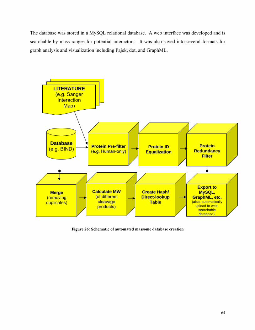
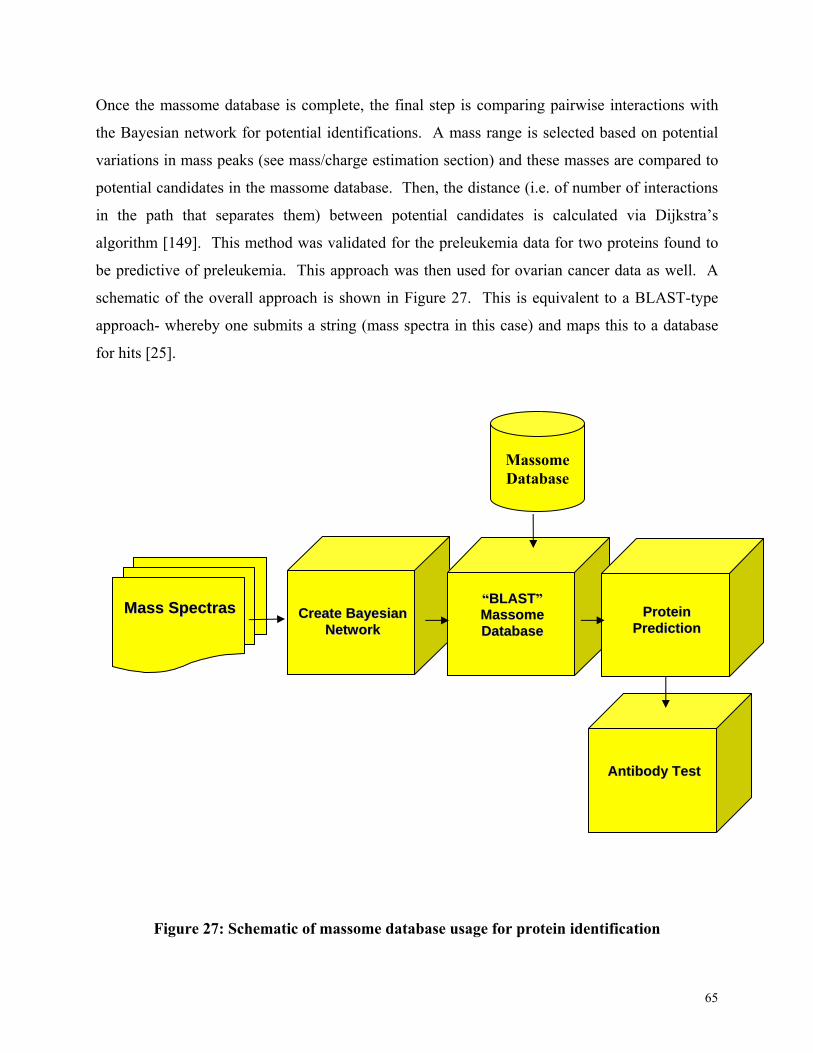
Once the massome database is complete, the final step is comparing pairwise interactions with

the Bayesian network for potential identifications. A mass range is selected based on potential

variations in mass peaks (see mass/charge estimation section) and these masses are compared to

potential candidates in the massome database. Then, the distance (i.e. of number of interactions

in the path that separates them) between potential candidates is calculated via Dijkstra’s

algorithm [149]. This method was validated for the preleukemia data for two proteins found to

be predictive of preleukemia. This approach was then used for ovarian cancer data as well. A

schematic of the overall approach is shown in Figure 27. This is equivalent to a BLAST-type

approach- whereby one submits a string (mass spectra in this case) and maps this to a database

for hits [25].

Figure 27: Schematic of massome database usage for protein identification

CCrreeaattee BBaayyeessiiaann NNeettwwoorrkk

Massome Database

““BBLLAASSTT”” MMaassssoommee DDaattaabbaassee

MMaassss SSppeeccttrraass

PPrrootteeiinn PPrreeddiiccttiioonn

AAnnttiibbooddyy TTeesstt

66

After creating a Bayesian network as described in section IV.B, the next step was to try to

predict the chemokines (e.g. for preleukemia) using the aforementioned Bayesian network links

and mapping them to the massome. To do this, the massome database was developed as just

described above. For visualization purposes, a 3-D version Fruchterman-Reingold force-directed

placement algorithm [154] was used to plot a human massome subset within the Pajek

environment [155] (see Figure 28). The outer ‘cortex’ potion of the cube contains the proteins

vertices, while the inner ‘medulla’ contains interaction edges.

A public, searchable version of the humans massome database has been made available at

www.chip.org/proteomics/massome.html

Using the human massome database, candidates for the identity of Chemokines A and B where

proposed as shown in Figure 29. Under the ‘other’ category, there were seven results that

included unconnected proteins in the graph. In Figure 29, Proteins A and B can be seen in the

list and the identity of both together (second to last row in the figure) was also one of the

predictions. In fact, more than half of the possibilities shown in the figure would have yielded

Figure 28: 3-D visualization of a portion of the human massome of protein interactions

67

at least one novel, identified, and differentially expressed protein via a simple antibody test.

The Chemokine A and B identities were found to be correctly predicted.

Based on the Bayesian network for the ovarian cancer dataset (see Figure 15), several peaks of

interest were selected based on disease prediction. The resulting identification is shown in

Figure 30 for the 6899.54 and 8602.384 m/z peak nodes. The ‘other’ category includes 20

other results of proteins not connected in the graph.

Interactor A Interactor B Dijkstra Distance ID

Chemokine, CC motif, ligand 3 like protein 1 Translocase of inner mitochondrial membrane 8 homolog B; 6Chemokine, CC motif, ligand 3 like protein 1 Apolipoprotein C-I 6Chemokine, CC motif, ligand 3 like protein 1 CCL13 2Chemokine, CC motif, ligand 3 like protein 1 Chemokine B 4Chemokine A Translocase of inner mitochondrial membrane 8 homolog B; 6Chemokine A Apolipoprotein C-I 5Chemokine A CCL13 5Chemokine A Chemokine B 7 XOther Other Infinity

Figure 29: Validation of interaction predictive ability in preleukemia dataset

Interactor A Interactor B Dijkstra Distance

Amyloid beta A4 protein precursor Amyloid Beta A4 Precursor Protein-Binding Family A Member 2 2Amyloid beta A4 protein precursor Polyubiquitin UbC 310 KDa Heat Shock Protein Polyubiquitin UbC 3Amyloid beta A4 protein precursor Heat shock factor binding protein 1 510 KDa Heat Shock Protein Amyloid Beta A4 Precursor Protein-Binding Family A Member 2 510 KDa Heat Shock Protein heat shock factor binding protein 1 510 KDa Heat Shock Protein Interferon gamma-induced precursor 5Amyloid beta A4 protein precursor Interferon gamma-induced precursor 6Other Other Infinity

Figure 30: Prediction example for ovarian cancer dataset

68

CHAPTER V: CONCLUSION AND DISCUSSION

V.A. Summary and Contributions

This section summarizes the issues explored in this work. It then outlines the contributions

contained within this thesis and its results.

V.A.1. SUMMARY

The contribution of genomics in understanding the human proteome has been invaluable.

However, perhaps greatest potential lies in the diversity of the full set of protein products and

their interactions. As the number of proteins being cataloged in databases continues to grows

exponentially while the estimates of the number of genes in humans and other organisms actually

declines, there is a burgeoning need for proteomics and methods to make use of this information.

As such, new statistical and engineering-based methods were proposed here to deal with this new

information.

Proteins’ abundance, miniature size, and dynamic nature have made them difficult to analyze.

On the other hand, these features also make proteins the perfect complex system for engineering-

based analysis. While some of the fundamental physics of mass spectrometry technologies used

to investigate proteins have been worked out, not all of details are known. For example, the

models for the mechanism of ionization have not proved sufficient in predicting spectra

accurately (which influences the m/z ratio). Also, concentration cannot be used solely to predict

the intensity of the associated peaks- as numerous other variables are involved such as solution

composition and mass spectrometry behavior [156]. Yet, even if the intensity can be associated

with one protein mass, there are still challenges in associating this with a unique protein. While

MS/MS techniques typically use Sequest-like methods for peptides, SELDI-TOF techniques

69

typically cannot (due to the lack of the second mass spectrometry signal information). As a

result, mostly proteomic profiles have been reported rather than in-depth analysis of the proteins.

Here, Bayesian-based analysis was used to look at protein identification. By combining

networks derived from SELDI mass spectra data with ones extracted from protein interactions, a

method for protein identification was proposed and confirmed via real clinical and mass

spectrometry-based data. In the process, a number of other related findings were delineated.

Beyond the overall unified Bayesian framework, a supporting statistical signal processing

methodology was developed to isolate potential proteins from the actual mass spectrometry data.

This was used to separate mass from charge by resolving both cases of peak-protein ambiguities

(via an estimation model and Bayesian network/Markov blanket respectively).

Validation was done with real preleukemia samples; novel predictions and explanations of

biomarker peaks were proposed for a previously published ovarian cancer dataset.

V.A.2. CONTRIBUTIONS

This work introduces a new way of deconvolving mass from charge and computationally

identifying proteins from their network-associated topology. This work establishes a Bayesian

framework that allows one to translate a disease-based mass spectrometry peak profile to useful

protein identifications. It is based on the novel idea that proteins can be identified by the

perturbations that they create in the network of proteins that they are associated with. Using this

notion, one can compare networks in different states (e.g. disease/control) and determine the

relationships in the network- thus isolating and identifying relevant proteins. On a higher level

of abstraction, this introduces a new way of using Bayesian-based analysis to learn node

identities by comparing inter-network links. Normally, intra-network links are learned by

comparing node-based information in Bayesian analysis.

70

V.B. Implications and Limitations

This work has a number of implications for mass-based proteomics. These are explored below.

Also, as with any method, there are certain assumptions and limitations. Some of these can be

dealt with in future work- as outlined in the next section.

V.B.1. IMPLICATIONS

This research shows how new computational methods can change the way proteomics is done by

validating and generating new hypotheses. Using the protein identification method discussed in

this thesis can reduce time and costs. It took half a year to determine the two proteins

biologically, yet the computational time to propose candidates was on the order of hours to days.

Antibodies experiments, which can be done in time on the order of hours for a few hundred

dollars each, can be used to biologically confirm any predictions made by the method. While

this thesis focused on SELDI technology, several aspects of the framework can be extended to

tandem MS technologies.

As seen in this thesis, the implications of this work are that future research in proteomics needs

to build and leverage on a given technology’s strengths while at the same time integrating other

data sources- to make the best possible use of available information. Both engineering and

scientific expertise are needed in evaluating the conclusions. For example, determining the

validity and relevance of proteins requires biological expertise while the design of a protein array

or statistical algorithm requires a different technical background. Thus, making good use of

information gleaned during such experiments requires innovative approaches ranging from

constructing accurate models to better experimental hypotheses.

V.B.2. LIMITATIONS

As with any method, the ones proposed in this thesis have their limitations. Some of these are

due to the nature of the data available, while others are related to simplifying assumptions. The

71

mass spectrometry data is inherently noisy. While papers claim 100-400 ppm mass variability

for mass drift of high resolution instruments, the actual peak variability turned out to be much

greater with posttranslational modifications and blurring of peaks. Thus, even if more values are

recorded at high resolution, there is still interference between peaks due to Gaussian peak

spreading. We also do not explicitly look for posttranslational modifications. However, this

constraint can be relaxed via manual searching for modifications with databases such as RESID

[157].

In terms of assumptions, the thesis looked at pairwise protein interactions. In reality, proteins

can work together in large complexes and this can be used to aid in protein identification (see

future work section). If needed, the proteins can be constrained via different SELDI surfaces

(e.g. using antibody-laden surface, etc.).

V.C. Future Work and Conclusion

This section discusses the possibilities for future work in this area. It then concludes with some

closing remarks on the topic of using protein identification in proteomics with clinical

applications.

V.C.1. FUTURE WORK

Much of the future work is related to minimizing assumptions and constraints. For example, to

mitigate peak spreading issues due to posttranslational modifications, pre-filtering of the

biological sample (e.g. to bind phosphorylated proteins, etc.) can be done. Also, development of

more accurate filtering within the mass spectrometry instrument can help to separate between

ionized clouds of proteins with similar mass (e.g. by isotope-based labeling or using other

protein properties than mass/charge).

By considering multiple (rather than pairwise) protein interactions, more constraints on protein

identity can be imposed- thus further reducing the number of proposed candidates for each

72

protein. For example, if a path involving two complexes of proteins is found to be activated in

common with several proteins in the network, then proteins within this complex may be more

likely involved (as opposed to uncomplexed proteins).

Integration of microarray and/or tissue-specific interaction data can provide more information on

about protein relationships under specific constraints. For this work, only protein-protein

interactions were examined. In the future, it would be useful to include other molecular

interactions such as DNA-protein binding.

V.C.2. CONCLUSION

This work presents methods that allow for novel ways to analyze SELDI mass spectrometry data.

It establishes a unified framework that permits analysis at several levels- from pathology-based

Bayesian networks to individual proteins. It provides a computational framework for protein

identification based on network analysis. The method is tested using real, clinically-based

samples. Identifications are confirmed- and new disease markers are proposed. This work has

the potential of changing the field by transforming black box models into meaningful protein-

based models. SELDI proteomics will thus not just validate hypotheses, but also generating new

ones. Applications include all areas where mass-based proteomics has been applied, including

disease diagnosis, prognosis, and treatment. HIV, neoplastic entities (i.e. cancer), and

immunological disorders are some examples of targets for clinical proteomics. Through these

medical applications, proteomics can be used to change the way scientists and clinicians view

cellular function and disease.

73

CHAPTER VI: REFERENCES

1. Human Genome Sequencing Consortium, I., Finishing the euchromatic sequence of the

human genome. Nature, 2004. 431(7011): p. 931-45.

2. Crick, F.H.C., Central dogma of molecular biology. Nature, 1970. 227: p. 561-563.

3. Petricoin, E.F., et al., Clinical proteomics: translating benchside promise into bedside

reality. Nat Rev Drug Discov, 2002. 1(9): p. 683-95.

4. Issaq, H.J., et al., SELDI-TOF MS for diagnostic proteomics. Anal Chem, 2003. 75(7): p.

148-155.

5. Xu, X.Q., et al., Molecular classification of liver cirrhosis in a rat model by proteomics

and bioinformatics. Proteomics, 2004. 4(10): p. 3235-45.

6. Interewicz, B., et al., Profiling of normal human leg lymph proteins using the 2-D

electrophoresis and SELDI-TOF mass spectrophotometry approach. Lymphology, 2004.

37(2): p. 65-72.

7. Petricoin, E.F. and L.A. Liotta, SELDI-TOF-based serum proteomic pattern diagnostics

for early detection of cancer. Curr Opin Biotechnol, 2004. 15(1): p. 24-30.

8. Alterovitz, G., et al. Machine Learning Techniques for Proteomic Classification and

Marker Selection Using Sample Fractionation with SELDI-TOF MS. in International

Conference on Analysis of Genomic Data. 2004. Boston, MA.

9. Sebastiani, P., et al., Genetic dissection and prognostic modeling of overt stroke in sickle

cell anemia. Nat Genet, 2005. 37(4): p. 435-40.

10. Troyanskaya, O.G., et al., A Bayesian framework for combining heterogeneous data

sources for gene function prediction (in Saccharomyces cerevisiae). Proc Natl Acad Sci

U S A, 2003. 100(14): p. 8348-53.

11. Ramoni, M.F., P. Sebastiani, and I.S. Kohane, Cluster analysis of gene expression

dynamics. Proc Natl Acad Sci U S A, 2002. 99(14): p. 9121-6.

12. Alterovitz, G., E. Afkhami, and M. Ramoni, Robotics, Automation, and Statistical

Learning for Proteomics, in Trends in Robotics, P.J. Benne, Editor. 2005 (In press), Nova

Science Publishers, Inc.: New York.

74

13. Banks, R.E., et al., Proteomics: new perspectives, new biomedical opportunities. Lancet,

2000. 356(9243): p. 1749-56.

14. Cox, D.R., et al., Assessing mapping progress in the Human Genome Project. Science,

1994. 265(5181): p. 2031-2.

15. Lander, E.S., et al., Initial sequencing and analysis of the human genome. Nature, 2001.

409(6822): p. 860-921.

16. DeRisi, J., et al., Use of a cDNA microarray to analyse gene expression patterns in

human cancer. Nat Genet, 1996. 14(4): p. 457-60.

17. Kononen, J., et al., Tissue microarrays for high-throughput molecular profiling of tumor

specimens. Nat Med, 1998. 4(7): p. 844-7.

18. Lander, E.S., The new genomics: global views of biology. Science, 1996. 274(5287): p.

536-9.

19. Friedman, N., et al., Using Bayesian networks to analyze expression data. J Comput Biol,

2000. 7(3-4): p. 601-20.

20. Segal, E., et al., A module map showing conditional activity of expression modules in

cancer. Nat Genet, 2004. 36(10): p. 1090-8.

21. Yarmush, M. and A Jayaraman, Advances in Proteomic Technologies. Annu Rev Biomed

Eng, 2002. 4: p. 349-373.

22. Petricoin, E.F., 3rd, et al., Serum proteomic patterns for detection of prostate cancer. J

Natl Cancer Inst, 2002. 94(20): p. 1576-8.

23. Petricoin, E.F., et al., Use of proteomic patterns in serum to identify ovarian cancer.

Lancet, 2002. 359(9306): p. 572-7.

24. Sorace, J.M. and M. Zhan, A data review and re-assessment of ovarian cancer serum

proteomic profiling. BMC Bioinformatics, 2003. 4(1): p. 24.

25. Wheeler, D.L., et al., Database resources of the National Center for Biotechnology

Information. Nucleic Acids Res, 2005. 33(Database issue): p. D39-45.

26. Wilkins, M.R., From proteins to proteomes: large scale protein identification by two

dimensional electrophoresis and amino acid analysis. Biotechnology, 1996. 14: p. 61-65.

27. Mootha, V.K., et al., Integrated analysis of protein composition, tissue diversity, and

gene regulation in mouse mitochondria. Cell, 2003. 115(5): p. 629-40.

75

28. Wadsworth, J.T., et al., Serum protein profiles to identify head and neck cancer. Clin

Cancer Res, 2004. 10(5): p. 1625-32.

29. Carrette, O., et al., A panel of cerebrospinal fluid potential biomarkers for the diagnosis

of Alzheimer's disease. Proteomics, 2003. 3(8): p. 1486-94.

30. Dare, T.O., et al., Application of surface-enhanced laser desorption/ionization technology

to the detection and identification of urinary parvalbumin-alpha: a biomarker of

compound-induced skeletal muscle toxicity in the rat. Electrophoresis, 2002. 23(18): p.

3241-51.

31. Mukhopadhyay, T.K., et al., Rapid characterisation of outer membrane proteins in

Neisseria lactamica by surface enhanced laser desorption and ionisation - time of flight

mass spectroscopy for use in a meningococcal vaccine. Biotechnol Appl Biochem, 2004.

32. Gravett, M.G., et al., Diagnosis of intra-amniotic infection by proteomic profiling and

identification of novel biomarkers. Jama, 2004. 292(4): p. 462-9.

33. Xiao, Z., et al., Serum proteomic profiles suggest celecoxib-modulated targets and

response predictors. Cancer Res, 2004. 64(8): p. 2904-9.

34. Boot, R.G., et al., Marked elevation of the chemokine CCL18/PARC in Gaucher disease:

a novel surrogate marker for assessing therapeutic intervention. Blood, 2004. 103(1): p.

33-9.

35. Anderson, N.L., et al., The human plasma proteome: a nonredundant list developed by

combination of four separate sources. Mol Cell Proteomics, 2004. 3(4): p. 311-26.

36. Davis, M.T., et al., Towards defining the urinary proteome using liquid chromatography-

tandem mass spectrometry. II. Limitations of complex mixture analyses. Proteomics,

2001. 1(1): p. 108-17.

37. Spahr, C.S., et al., Towards defining the urinary proteome using liquid chromatography-

tandem mass spectrometry. I. Profiling an unfractionated tryptic digest. Proteomics,

2001. 1(1): p. 93-107.

38. Hanash, S., Disease proteomics. Nature, 2003. 422: p. 226-32.

39. D.D. Shoemaker P.S. Linsley Recent developments in DNA microarrays. Current

Opinion in Microbiology, 2002. 5: p. 334-7.

40. Templin, M.F., et al., Protein microarrays and multiplexed sandwich immunoassays:

what beats the beads? Comb Chem High Throughput Screen, 2004. 7(3): p. 223-9.

76

41. Nielsen, U.B. and B.H. Geierstanger, Multiplexed sandwich assays in microarray format.

J Immunol Methods, 2004. 290(1-2): p. 107-20.

42. Xu, Q. and K.S. Lam, Protein and chemical microarrays-powerful tools for proteomics.

Journal of Biomedicine & Biotechnology, 2003. 2003(5): p. 257-66.

43. Hosokawa, Y., et al. Fabrication and application of protein crystal microarrays. in

Bioinspired Nanoscale Hybrid Systems. Symposium, 2-4 Dec. 2002. 2003. Boston, MA,

USA: Mater. Res. Soc.

44. Smith, J.T. and W.M. Reichert. The optimization of quill-pin printed protein and DNA

microarrays. in Conference Proceedings. Second Joint EMBS-BMES Conference 2002

24th Annual International Conference of the Engineering in Medicine and Biology

Society. Annual Fall Meeting of the Biomedical Engineering Society, 23-26 Oct. 2002.

2002. Houston, TX, USA: IEEE.

45. Gosalia, D.N. and S.L. Diamond. High throughput screening using enzyme assay

microarrays. in Conference Proceedings. Second Joint EMBS-BMES Conference 2002

24th Annual International Conference of the Engineering in Medicine and Biology

Society. Annual Fall Meeting of the Biomedical Engineering Society, 23-26 Oct. 2002.

2002. Houston, TX, USA: IEEE.

46. Lee, K.-N., et al., Micromirror array for protein micro array fabrication. Journal of

Micromechanics and Microengineering, 2003. 13(3): p. 474-81.

47. Jin, G., et al. Immune-microassay with optical proteinchip for protein detection. in

Proceedings of the 25th Annual International Conference of the IEEE Engineering in

Medicine and Biology Society, 17-21 Sept. 2003. 2003. Cancun, Mexico: IEEE.

48. Najmabadi, P., A.A. Goldenberg, and A. Emili, Conceptual design for an automated

high-throughput magnetic protein complex purification workcell. JALA, 2003. 8(6): p.

101-6.

49. Muthusubramaniam, L., et al. Automating crystallization of membrane proteins by robot

with soft coordinate measuring. in 2004 IEEE International Conference on Robotics and

Automation, 26 April-1 May 2004. 2004. New Orleans, LA, USA: IEEE.

50. Kazerounian, K., From mechanisms and robotics to protein conformation and drug

design. Transactions of the ASME. Journal of Mechanical Design, 2004. 126(1): p. 40-5.

77

51. Lee, W.C. and Y.-H. Cho. Nanomechanical protein detectors using electrothermal nano-

gap actuators. in 17th IEEE International Conference on Micro Electro Mechanical

Systems. Maastricht MEMS 2004 Technical Digest, 25-29 Jan. 2004. 2004. Maastricht,

Netherlands: IEEE.

52. Pan, Y.V., et al. A precision technology for controlling protein adsorption and cell

adhesion in bioMEMS. in Technical Digest. MEMS 2001. 14th IEEE International

Conference on Micro Electro Mechanical Systems, 21-25 Jan. 2001. 2001. Interlaken,

Switzerland: IEEE.

53. Song, G. and N.M. Amato. A motion planning approach to folding: from paper craft to

protein folding. in Proceedings 2001 ICRA. IEEE International Conference on Robotics

and Automation, 21-26 May 2001. 2001. Seoul, South Korea: IEEE.

54. Song, G. and N.M. Amato, A motion-planning approach to folding: from paper craft to

protein folding. IEEE Transactions on Robotics and Automation, 2004. 20(1): p. 60-71.

55. Bertone, P. and M. Gerstein, Integrative data mining: the new direction in

bioinformatics. IEEE Engineering in Medicine and Biology Magazine, 2001. 20(4): p.

33-40.

56. Kohlbacher, O. and K. Reinert, Differential analysis in proteomics: experimental

methods, algorithmic challenges. IT-Information Technology, 2004. 46(1): p. 31-8.

57. Hai-ting, Z., Machine learning and bioinformatics. Information and Control, 2003. 32(4):

p. 352-7.

58. Alterovitz, G., et al., Analysis and Robot Pipelined Automation for SELDI-TOF Mass

Spectrometry. Proceedings of the International Conference of IEEE Engineering in

Medicine and Biology, San Francisco, CA, USA, 2004.

59. Anderson, A. and Z. Weng, VRDD: applying virtual reality visualization to protein

docking and design. Journal of Molecular Graphics & Modelling, 1999. 17(3-4): p. 180-

6.

60. Fellenberg, M., et al. Integrative analysis of protein interaction data. in Proceedings of

the Eighth International Conference on Intelligent Systems for Molecular Biology, 16-23

Aug. 2000. 2000. La Jolla, CA, USA: AAAI Press.

61. Han, K. and Y. Byun, Three-dimensional visualization of protein interaction networks.

Computers in Biology and Medicine, 2004. 34(2): p. 127-39.

78

62. D. Hirschberg S. Tryggvason M. Gustafsson M, Identification of endothelial proteins by

MALDI-MS using a compact disc microfluidic system. Protein Journal, 2004. 23: p. 263-

71.

63. Mann, M.T.M., From genomics to proteomics. Nature, 2003. 422: p. 193-197.

64. S.F. Altschul T.L. Madden A.A. Schaffer J. Zhang Z. Zhang W. Miller D.J. Lipman,

Gapped BLAST and PSI-BLAST: a new generation of protein database search programs.

Nucleic Acid Research, 1997. 17: p. 3389-402.

65. Genome sequence of the nematode C. elegans: a platform for investigating biology. The

C. elegans Sequencing Consortium. Science, 1998. 282(5396): p. 2012-8.

66. S. P. Gygi Y. Rochon B. R. Franza R. Aebersold, Correlation between Protein and

mRNA Abundance in Yeast. Molecular and Cellular Biology, 1999. 19: p. 1720-30.

67. C. Hoog, M.M., Proteomics. Annual review of Genomics and human Genetics, 2004. 5:

p. 267-93.

68. Williams, V., Pathways of Innovation: a history of the first effective treatment for sickle

cell anemia. Perspect Biol Med., 2004. 4(47): p. 552-63.

69. Chapman, T., Automation on the move. Nature, 2003. 421: p. 661 - 66.

70. Bachrach, C.A. and T. Charen, Selection of MEDLINE contents, the development of its

thesaurus, and the indexing process. Med Inform (Lond), 1978. 3(3): p. 237-54.

71. Glover, J., Searching for the evidence using PubMed. Med Ref Serv Q, 2002. 21(4): p.

57-65.

72. Bachmann, L.M., et al., Identifying diagnostic studies in MEDLINE: reducing the

number needed to read. J Am Med Inform Assoc, 2002. 9(6): p. 653-8.

73. A.W. Dowsey M.J. Dunn G.Z. Yang, ProteomeGRID: towards a high-throughput

proteomics pipeline through opportunistic cluster image computing for two-dimensional

gel electrophoresis. Proteomics, 2004.

74. M. Traini AA. Gooley K. Ou, Towards an automated approach for protein

identification in proteome projects. Electrophoresis, 1998. 11: p. 1941-9.

75. C.R. Mallet Z. Lu R. Fisk J.R. Mazzeo, Performance of an ultra-low elution-volume 96-

well plate: drug discovery and development applications. Rapid Communications in

Mass Spectrometry, 2003. 17: p. 163-70.

76. www.thermo.com, Thermo Electron,. 2004.

79

77. Choudum, S.A. and S. Sivagurunathan, Optimal fault-tolerant networks with a server.

Networks, 2000. 35(2): p. 157-60.

78. Mahgoub, I. and C.-J. Huang, A novel scheme to improve fault-tolerant capabilities of

multistage interconnection networks. Telecommunication Systems - Modeling, Analysis,

Design and Management, 1998. 10(1-2): p. 45-66.

79. Yang, S.-C. and J.A. Silvester, Fault-tolerant multistage interconnection networks:

performance/reliability tradeoffs. Computer Systems Science and Engineering, 1990.

5(4): p. 233-42.

80. Arpinar, I.B., et al., Formalization of workflows and correctness issues in the presence of

concurrency. Distributed and Parallel Databases, 1999. 7(2): p. 199-248.

81. Ceroni, J.A. and S.Y. Nof, A workflow model based on parallelism for distributed

organizations. Journal of Intelligent Manufacturing, 2002. 13(6): p. 439-61.

82. Mahling, D.E., N. Craven, and W.B. Croft, From office automation to intelligent

workflow systems. IEEE Expert, 1995. 10(3): p. 41-7.

83. Rajakumar, S., V.P. Arunachalam, and V. Selladurai, Workflow balancing strategies in

parallel machine scheduling. International Journal of Advanced Manufacturing

Technology, 2004. 23(5-6): p. 366-74.

84. H. Liu D Lin J.R. Yates 3rd, Multidimensional separations for protein/peptide analysis

in the post-genomic era. Biotechniques, 2002. 32: p. 898-902.

85. Leibler, Introduction to Proteomics: Tools for the New Biology. 2002, Totowa, NJ:

Humana Press.

86. P. Wickware P. Smaglik, Proteomics technology: Character references. 2001. 413: p.

869 - 875.

87. Mitra S Brukh R, Sample Preparation Techniques in Analytical Chemistry. 2003: John

Wiley & Sons.

88. Ruedi Aebersold, M.M., Mass spectrometry-based proteomics. Nature, 2003. 422: p. 198

- 207.

89. M. Yarmush A Jayaraman, Advances in Proteomic Technologies. Annual review of

Biomedical Engineering, 2002. 4: p. 349-373.

90. G.A. Michaud M. Snyder, Proteomic Approaches for the Global Analysis of Proteins.

Biotechniques, 2002. 33: p. 1308-16.

80

91. John R Yates, Mass Spectrometry and the Age of the Proteome. Journal of Mass

Spectrometry, 1998. 33: p. 1-19.

92. Dalmasso, G.R.E.A., SELDI ProteinChip Array Technology: Protein-Based predictive

Medicine and Drug Discovery Applications. Journal of Biomedicine and Biotechnology,

2003. 4: p. 237-41.

93. Conrads, T.P., et al., High-resolution serum proteomic features for ovarian cancer

detection. Endocr Relat Cancer, 2004. 11(2): p. 163-78.

94. Marshall, A.G., Accounts of Chemical Research, 1996. 29: p. 308.

95. Lahm H-W, L.H., Mass spectrometry: a tool for the identification of proteins separated

by gels. 2000. 21: p. 2105-14.

96. Mann M, H.R., Pandey A, Analysis of proteins and proteomes by mass spectrometry.

Annual. Rev. Biochem, 2001. 70: p. 437-73.

97. Kuster B, M.P., Andersen JS, Mann M, Mass spectrometry allows direct identification of

proteins in large genomes. Proteomics, 2001. 1: p. 641-50.

98. Pappin DJ, H.P., Bleasby AJ, Rapid identification of proteins by peptide-mass

fingerprinting. Curr Biol, 1993. 3: p. 327-32.

99. Eng J, M.A., Yates JR, An approach to correlate tandem mass spectral data of peptides

with amino acid sequences in a protein database. J. Am. Soc. Mass Spectrom, 1994. 5: p.

976-89.

100. Quadroni M, J.P., Proteomics and automation. Electrophoresis, 1999. 20: p. 664-77.

101. JR Yates, Database searching using mass spectrometry data. Electrophoresis, 1998. 19:

p. 893-900.

102. Lill, J., Proteomic tools for quantitation by mass spectrometry. Mass Spectrom. Rev,

2003. 22: p. 182-94.

103. Brooksbank, C., G. Cameron, and J. Thornton, The European Bioinformatics Institute's

data resources: towards systems biology. Nucleic Acids Res, 2005. 33(Database issue):

p. D46-53.

104. Bourne, P.E., J. Westbrook, and H.M. Berman, The Protein Data Bank and lessons in

data management. Brief Bioinform, 2004. 5(1): p. 23-30.

81

105. Xenarios, I., et al., DIP, the Database of Interacting Proteins: a research tool for

studying cellular networks of protein interactions. Nucleic Acids Res, 2002. 30(1): p.

303-5.

106. Alfarano, C., et al., The Biomolecular Interaction Network Database and related tools

2005 update. Nucleic Acids Res, 2005. 33(Database issue): p. D418-24.

107. Hermjakob, H., et al., The HUPO PSI’s molecular interaction format–a community

standard for the representation of protein interaction data. Nat Biotechnol, 2004. 22: p.

177-83.

108. Bairoch, A., et al., The Universal Protein Resource (UniProt). Nucleic Acids Res, 2005.

33(Database issue): p. D154-9.

109. Hubbard, T., et al., Ensembl 2005. Nucleic Acids Res, 2005. 33(Database issue): p.

D447-53.

110. Kersey, P.J., et al., The International Protein Index: an integrated database for

proteomics experiments. Proteomics, 2004. 4(7): p. 1985-8.

111. Prince, J.T., et al., The need for a public proteomics repository. Nat Biotechnol, 2004.

22(4): p. 471-2.

112. Michalickova, K., et al., SeqHound: biological sequence and structure database as a

platform for bioinformatics research. BMC Bioinformatics, 2002. 3(1): p. 32.

113. Iragne, F., et al., AliasServer: a web server to handle multiple aliases used to refer to

proteins. Bioinformatics, 2004. 20(14): p. 2331-2.

114. D.N. Chakravarti B. Chakravarti I. Moutsatsos, Informatic tools for proteome profiling.

Biotechniques, 2002. Suppl 32: p. 4-15.

115. D.N. Perkins D.J. Pappin D.M. Creasy J.S. Cottrell, Probability-based protein

identification by searching sequence databases using mass spectrometry data.

Electrophoresis, 1999. 18: p. 3551-67.

116. W Zhang B.T. Chait, ProFound: an expert system for protein identification using mass

spectrometric peptide mapping information. Analytical Chemistry, 2000. 72(11): p.

2482-89.

117. J.R. Yates J.K. Eng A.L. McCormack D. Schieltz, Method to Correlate Tandem Mass

Spectra of Modified Peptides to Amino Acid Sequences in the Protein Database.

Analytical Chemistry, 1995. 67: p. 1426-36.

82

118. J.R. Yates J.K. Eng A.L. McCormack, Mining genomes: Correlating Tandem Mass

Spectra of Modified and Unmodified Peptides to Sequences in Nucleotide Databases.

Analytical Chemistry, 1995. 67: p. 3202-10.

119. B.T. Hansen J.A. Jones D.E. Mason D.C. Liebler, SALSA: a pattern recognition

algorithm to detect electrophile-adducted peptides by automated evaluation of CID

spectra in LC-MS-MS analyses. Analytical Chemistry, 2001. 73: p. 1676-83.

120. D.C. Liebler B.T. Hansen S.W. Davey L. Tiscareno D.E. Mason, Peptide sequence motif

analysis of tandem MS data with the SALSA algorithm. Analytical Chemistry, 2002. 74:

p. 203-10.

121. D.L. TaBB J.K. Eng J.R. Yates, Protein Identification by SEQUEST, in Proteome

Research: Mass Spectrometry, P. James, Editor. 2001, Springer. p. 125-42.

122. Poetz, O., et al., Protein microarrays for antibody profiling: Specificity and affinity

determination on a chip. Proteomics, 2005.

123. Legrain, P. and L. Selig, Genome-wide protein interaction maps using two-hybrid

systems. FEBS Lett, 2000. 480(1): p. 32-6.

124. A. Barabasi Z. Oltvai, Network biology: understanding the cell's functional organization.

Nature rev. genetics, 2004. 5: p. 101-113.

125. R. Albert A.L. Barabasi, Statistical mechanics of complex networks. Rev. Modern

Physics, 2002. 74: p. 47-97.

126. Jain, A.K. and J. Mao, Artificial neural networks: A tutorial. IEEE Computer, 1996.

29(3): p. 31-44.

127. Cortes, C. and V. Vapnik, Support-vector networks. Machine Learning. 20(3): p. 273-97.

128. Goldberg, D., Genetic Algorithms in Search, Optimization, and Machine Learning. 1989:

Addison-Wesley.

129. Hartigan, J. and M. Wong, Algorithm AS136: A k-means clustering algorithm. Applied

Statistics, 1979. 28: p. 100-108.

130. Joliffe, I., Principal Component Analysis. 1986, New York, NY: Springer-Verlag.

131. Jain, A. and R. Dubes, Algorithms for Clustering Data. 1988, Englewood Cliffs, NJ.:

Prentice-Hall.

83

132. Cheeseman, P., Stutz, J., Bayesian Classification (Autoclass): Theory and Results, in

Advances in Knowledge Discovery and Data Mining, G.P.-S. U. Fayyad, P. Smyth and R.

Uthurusamy, Editor. 1996, MIT Press: Cambridge.

133. Samso, M., et al., A Bayesian method for classification of images from electron

micrographs. J Struct Biol, 2002. 138(3): p. 157-70.

134. Nigam, K., et al., Text classification from labeled and unlabeled documents using EM.

Machine Learning, 2000. 39(2-3): p. 103-34.

135. Gelman, A., et al., Bayesian data analysis. 1995, New York: Chapman & Hall.

136. Aivado, M., et al., Optimization and evaluation of surface-enhanced laser

desorption/ionization time-of-flight mass spectrometry (SELDI-TOF MS) with reversed-

phase protein arrays for protein profiling. Clin Chem Lab Med, 2005. 43(2): p. 133-40.

137. Cooper, G.F. and E. Herskovits, A Bayesian method for the induction of probabilistic

networks from data. Machine Learning, 1992. 9(4): p. 309-347.

138. Chickering, D.M., D. Geiger, and D. Heckerman, Learning Bayesian Networks is NP-

Hard, Technical Report MSR-TR-94-17. 1994, Microsoft Research.

139. Heckerman, D., A Tutorial on Learning With Bayesian Networks. Microsoft Research,

MSR-TR-95-06, 1995.

140. Ramoni, M.F. and P. Sebastiani, Learning Bayesian networks form incomplete databases.

UAI, 1997.

141. Ramoni, M.F. and P. Sebastiani, Bayesian Methods in Intelligent Data Analysis, in

Intelligent Data Analysis, An Introduction, M.R.B.a.D.J. Hand, Editor. 2003, Springer

Verlag: New York. p. 131–168.

142. Oppenheim, A.V., A.S. Willsky, and H. Nawab, Signals and Systems. 3rd ed. 1997,

Englewood Cliffs, NJ: Prentice Hall.

143. Pearl, J., Causality : Models, Reasoning, and Inference. 2000, Cambridge: Cambridge

University Press.

144. Jeong, H., et al., Lethality and centrality in protein networks. Nature, 2001. 411(6833): p.

41-2.

145. Yu, H., et al., TopNet: a tool for comparing biological sub-networks, correlating protein

properties with topological statistics. Nucleic Acids Res, 2004. 32(1): p. 328-37.

84

146. Lehner, B. and A.G. Fraser, A first-draft human protein-interaction map. Genome Biol,

2004. 5(9): p. R63.

147. Alterovitz, G., et al. Human Protein Meta-Interaction Database (HPMD) Potentiates

Integration for Meta-Analysis. in IEEE GENSIPS. 2005 (accepted).

148. http://www.ncbi.nlm.nih.gov/entrez/query/static/help/helpdoc.html#Limits.

149. Ahuja, R.K., T.L. Magnanti, and J.B. Orlin, Network Flows: Theory, Algorithms, and

Applications. 1993, New Jersey: Prentice Hall.

150. MK, B. and L. PH, PSA in the screening,staging and follow up of early-stage prostate

cancer. World J Urol, 1989. 7: p. 7-11.

151. Clayton, D. p-values, false discovery rates, and Bayes factors: how should we assess the

"significance" of genetic associations? in European Mathematical Genetics Meeting.

2003. Cambridge, UK.

152. Goodman, S.N., Toward evidence-based medical statistics. 2: The Bayes factor. Ann

Intern Med, 1999. 130(12): p. 1005-13.

153. Aivado, M., et al. Serum protein profiling with mass spectrometry for the diagnosis of

Myelodysplastic Syndromes (MDS). in The American Society of Hematology- 46th

Annual Meeting. 2004. San Diego.

154. Fruchterman, T.M.J. and E.M. Reingold, Graph Drawing by Force-directed Placement.

Software: Practice and Experience, 1991. 21(11): p. 1129 - 1164.

155. Batagelj, V. and A. Mrvar, Pajek - Program for Large Network Analysis. Connections,

1998. 21(2): p. 47-57.

156. Gay, S., et al., Peptide mass fingerprinting peak intensity prediction: extracting

knowledge from spectra. Proteomics, 2002. 2(10): p. 1374-91.

157. Garavelli, J.S., The RESID Database of Protein Modifications: 2003 developments.

Nucleic Acids Res, 2003. 31(1): p. 499-501.

158. B. Alberts A. Johnson J. Lewis M. Raff K. Roberts P. Walter, Molecular Biology of The

Cell. 2002: Garland Science.

159. T. D. Pollard W.C. Earnshaw, Cell Biology. 2002: W.B. Saunders Company.

160. J.C. Venter M.D. Adams E.W. Myers P.W. Li et al, The sequence of the human

genome. Nature, 2001. 291: p. 1304-51.

85

161. US department of energy, The human genome project and beyond. 2003, US department

of energy. p. 1-12.

162. D. Eisenberg E.M. Marcotte I. Xenarios T.O. Yeates, Protein function in the post-

genomic era. Nature, 2000. 405: p. 823-26.

163. BlackStock, W.P.W., M. P, Proteomics: quantitative and physical mapping of cellular

proteins. Trends in Biotechnology, 1999. 17: p. 121-127.

164. K Machida, M.N., M Imaizumi, T Abe, Y Ohnishi, K Takagi, S Yoshii, M Hamaguchi,

Tyrosine phosphorylation in lung cancer as a prognostic marker. Cancer Detection and

Prevention, 1996. 5(20).

86

CHAPTER VII: ACKNOWLEDGEMENTS

I want to thank Prof. Marco Ramoni for supervising this thesis. He was more than a supervisor-

he was a mentor. Thank you to Prof. Isaac Kohane. He taught me how approach and explore the

key issues in biology. Through the PhD, Prof. Ramoni and Prof. Kohane really helped me to

understand how to use engineering concepts in order to solve biomedical problems. Through

their reflections, I also learned about life in general- and at the microcosm of Harvard Medical

School and MIT. Thank you for your inspiration!

I would like to thank Prof. Vidal for his important role in my thesis committee.

I would to thank my collaborators over the years- including Prof. Mike Sieden at MGH, HPCGG

(especially David Sarracino), and the BIDMC Genomics Center (Towia Libermann, Manuel

Aivado).

Thank you to Atul Butte. We started the same year in the MEMP program and I learned a lot

about many aspects of research and career directions from him.

Thank you to past and current co-ops who volunteered their time to work with me, namely Dima

Patek, Ehsan Afkhami, Ye Lu, and Mike Xiang.

Thank you to Ira Pekker for your help and understanding during my busy time finishing this

thesis.

Thank you to my parents Samuel and Dalia Alterovitz for their love and support.

Thank you to CHIP (Children’s Hospital Informatics Program) for creating and warm

environment that encourages collaborations and learning.

87

This work has been generously funded during my tenure at MIT by a National Defense Science

and Engineering Graduate Fellowship as well as a grant from the Whitaker Foundation. Thank

you to both of these organizations for their support. I would also like to thank sponsors of

graduate-level fellowships including (sponsor in parentheses): Fulbright (USA/Canada), Tau

Beta Pi Fellowship (TBP), MEMP Fellowship (MIT), and Cambridge Science Foundation Travel

Fellowship (CSF).

88

CHAPTER VIII: APPENDIX

VIII.A. Mathematical Notation

Term Explanation

X X is a vector with elements {X1, X2, …Xn}

X ⊥ Y

X and Y are independent

(X ⊥ Y) | Z

X and Y are conditionally independent

given Z

I0 Prior information

I1 Posterior information

89

VIII.B. Glossary

Term Explanation

ESI Electrospray ionization

FT-MS Fourier transform mass spectrometry

MALDI

Matrix assisted laser desorption/ionization

MS/MS

Tandem mass spectrometry (mass

spectrometry/ mass spectrometry)

PMF Peptide mass fingerprinting

Q-TOF Quadrupole time-of-flight

SELDI Surface-enhanced laser

desorption/ionization

TOF Time-of-flight

90

1 2 3 4 5 6 7 8 9