213 Arctic Sea Ice Decline: Observations, Projections, Mechanisms, and Implications Geophysical Monograph Series 180 This paper is not subject to U.S. copyright. Published in 2008 by the American Geophysical Union. 10.1029/180GM14 A Bayesian Network Modeling Approach to Forecasting the 21st Century Worldwide Status of Polar Bears Steven C. Amstrup Alaska Science Center, U.S. Geological Survey, Anchorage, Alaska, USA Bruce G. Marcot Pacific Northwest Research Station, USDA Forest Service, Portland, Oregon, USA David C. Douglas Alaska Science Center, U.S. Geological Survey, Juneau, Alaska, USA To inform the U.S. Fish and Wildlife Service decision, whether or not to list polar bears as threatened under the Endangered Species Act (ESA), we projected the status of the world’s polar bears (Ursus maritimus) for decades centered on future years 2025, 2050, 2075, and 2095. We defined four ecoregions based on current and projected sea ice conditions: seasonal ice, Canadian Archipelago, polar basin divergent, and polar basin convergent ecoregions. We incorporated general circulation model projections of future sea ice into a Bayesian network (BN) model structured around the factors considered in ESA decisions. This first-generation BN model combined empirical data, interpretations of data, and professional judgments of one polar bear expert into a probabilistic framework that identifies causal links between environmental stressors and polar bear responses. We provide guidance regarding steps necessary to refine the model, including adding inputs from other experts. The BN model projected extirpation of polar bears from the seasonal ice and polar basin divergent ecoregions, where ≈2/3 of the world’s polar bears currently occur, by mid century. Projections were less dire in other ecoregions. Decline in ice habitat was the overriding factor driving the model outcomes. Although this is a first-generation model, the dependence of polar bears on sea ice is universally accepted, and the observed sea ice decline is faster than models suggest. Therefore, incorporating judgments of multiple experts in a final model is not expected to fundamentally alter the outlook for polar bears described here. 1. INTRODUCTION Polar bears depend upon sea ice for access to their prey and for other aspects of their life history [Stirling and Ørit- sland, 1995; Stirling and Lunn, 1997; Amstrup, 2003]. Ob- served declines in sea ice availability have been associated
Transcript
213
Arctic Sea Ice Decline: Observations, Projections, Mechanisms, and ImplicationsGeophysical Monograph Series 180This paper is not subject to U.S. copyright. Published in 2008 by the American Geophysical Union.10.1029/180GM14
A Bayesian Network Modeling Approach to Forecasting the 21st Century Worldwide Status of Polar Bears
Steven C. Amstrup
Alaska Science Center, U.S. Geological Survey, Anchorage, Alaska, USA
Bruce G. Marcot
Pacific Northwest Research Station, USDA Forest Service, Portland, Oregon, USA
David C. Douglas
Alaska Science Center, U.S. Geological Survey, Juneau, Alaska, USA
To inform the U.S. Fish and Wildlife Service decision, whether or not to list polar bears as threatened under the Endangered Species Act (ESA), we projected the status of the world’s polar bears (Ursus maritimus) for decades centered on future years 2025, 2050, 2075, and 2095. We defined four ecoregions based on current and projected sea ice conditions: seasonal ice, Canadian Archipelago, polar basin divergent, and polar basin convergent ecoregions. We incorporated general circulation model projections of future sea ice into a Bayesian network (BN) model structured around the factors considered in ESA decisions. This first-generation BN model combined empirical data, interpretations of data, and professional judgments of one polar bear expert into a probabilistic framework that identifies causal links between environmental stressors and polar bear responses. We provide guidance regarding steps necessary to refine the model, including adding inputs from other experts. The BN model projected extirpation of polar bears from the seasonal ice and polar basin divergent ecoregions, where ≈2/3 of the world’s polar bears currently occur, by mid century. Projections were less dire in other ecoregions. Decline in ice habitat was the overriding factor driving the model outcomes. Although this is a first-generation model, the dependence of polar bears on sea ice is universally accepted, and the observed sea ice decline is faster than models suggest. Therefore, incorporating judgments of multiple experts in a final model is not expected to fundamentally alter the outlook for polar bears described here.
1. INTRODUCTION
Polar bears depend upon sea ice for access to their prey and for other aspects of their life history [Stirling and Ørit-sland, 1995; Stirling and Lunn, 1997; Amstrup, 2003]. Ob-served declines in sea ice availability have been associated
samstrup
Typewritten Text
Article should be cited as: Amstrup, S. C. , B. G. Marcot, and D. C. Douglas. 2008. A Bayesian Network Modeling Approach to Forecasting the 21st Century Worldwide Status of Polar Bears. Pages 213-268 In Eric. T. DeWeaver, Cecilia M. Bitz, and L.-Bruno Tremblay Eds. Arctic Sea Ice Decline: Observations, Projections, Mechanisms, and Implications. Geophysical Monograph 180. American Geophysical Union, Washington DC.
samstrup
Typewritten Text
samstrup
Typewritten Text
samstrup
Typewritten Text
samstrup
Typewritten Text
samstrup
Typewritten Text
samstrup
Typewritten Text
samstrup
Typewritten Text
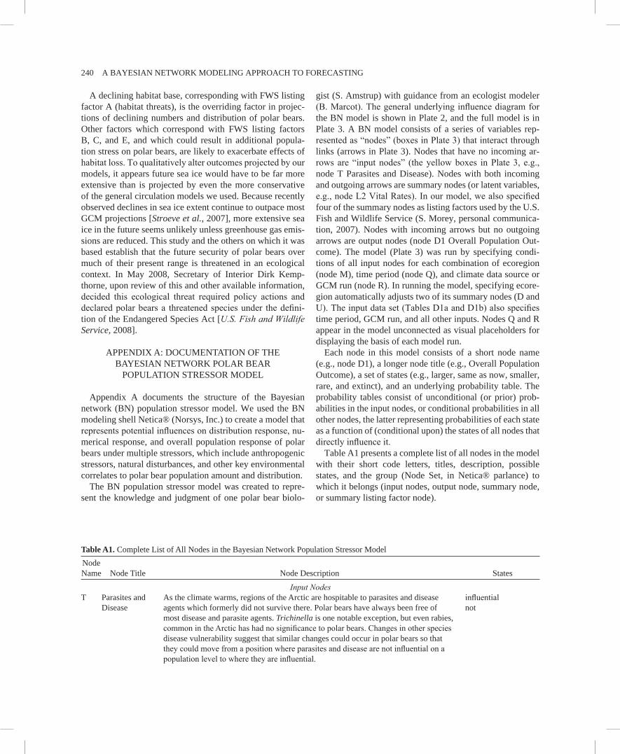
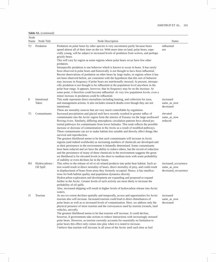
214 A BAyESIAN NETWORk MODElING APPROACh TO FORECASTING
with reduced body condition, reproduction, survival, and population size for polar bears in parts of their range [Stir-ling et al., 1999; Obbard et al., 2006; Stirling and Parkin-son, 2006; Regehr et al., 2007b]. Observed [Comiso, 2006] and projected [Holland et al., 2006] sea ice declines have led to the hypothesis that the future welfare of polar bears may be diminished worldwide and to the proposal by the U.S. Fish and Wildlife Service (FWS) to list the polar bear as a threatened species under the Endangered Species Act [U.S. Fish and Wildlife Service, 2007].
Classification as “threatened” requires determination that a species is likely to become “endangered” within the “fore-seeable future” throughout all or a significant portion of its range. An “endangered” species is any species that is in danger of extinction throughout all or a significant portion of its range. For polar bears, the “foreseeable future” was defined as 45 years from now [U.S. Fish and Wildlife Serv-ice, 2007]. here we describe a method for combining avail-able information on polar bear life history and ecology with projections of the future state of Arctic sea ice to project the future worldwide status of polar bears. We present our forecast in a “compared to now” setting where projections for the decade of 2045–2054 are compared to the “present” period of 1996–2006. For added perspective, we looked to the nearer term as well as beyond the defined foreseeable future by comparing projections for the periods 2020–2029, 2070–2079, and 2090–2099 to the present. Also, we looked back to the period of 1985–1995. hence we examined six time periods in total.
Our view of the present and past was based on sea ice con-ditions derived from satellite data. Our future forecasts were based on information derived from general circulation model (GCM) projections of the extent and spatiotemporal distri-bution of sea ice, our understanding of how polar bears have responded to ongoing changes in sea ice, and projections of how polar bears are likely to respond to future changes. This paper synthesizes information in nine Administrative Reports prepared by the U.S. Geological Survey and deliv-ered to the FWS in 2007 (http://www.usgs.gov/newsroom/ special/polar_bears/) plus other recent literature.
Polar bears occur throughout portions of the Northern hemisphere where the sea is ice covered for all or much of the year. Polar bears are thought to have branched off of brown bear (Ursus arctos) stocks as long ago as 250,000 years, but they appear in the fossil record no earlier than 120,000 years ago [Talbot and Shields, 1996; Hufthamer, 2001; Ingolfsson and Wiig, 2007]. Since moving offshore, behavioral and physical adaptations have allowed polar bears to increasingly specialize at hunting seals from the surface of the ice [Stirling, 1974; Smith, 1980; Stirling and Øritsland, 1995].
Over much of their range, polar bears are nutritionally de-pendent on the ringed seal (Phoca hispida). Polar bears oc-casionally catch belugas (Delphinapterus leucas), narwhals (Monodon monocerus), walrus (Odobenus rosmarus), and harbor seals (P. vitulina) [Smith, 1985; Calvert and Stirling, 1990; Smith and Sjare, 1990; Stirling and Øritsland, 1995; Derocher et al., 2002]. Walruses can be seasonally important in some parts of the polar bear range [Parovshchikov, 1964; Ovsyanikov, 1996]. Bearded seals (Erignathus barbatus) can be a large part of their diet where they are common and are probably the second most common prey of polar bears [De-rocher et al., 2002]. The most common prey of polar bears, however, is the ringed seal [Smith and Stirling, 1975; Smith, 1980]. The relationship between ringed seals and polar bears is so close that the abundance of ringed seals in some areas appears to regulate the density of polar bears, while polar bear predation, in turn, regulates density and reproductive success of ringed seals in other areas [Hammill and Smith, 1991; Stirling and Øritsland, 1995]. Across much of the polar bear range, their dependence on ringed seals is close enough that the abundances of ringed seals have been esti-mated by knowing the abundances of polar bears [Stirling and Øritsland, 1995; Kingsley, 1998]. Although polar bears occasionally catch seals on land or in open water [Furnell and Oolooyuk, 1980], they consistently catch seals and other marine mammals only at the air-ice-water interface.
like all bears, polar bears are opportunistic and will take a broad variety of foods when available. When stranded on land for long periods polar bears will consume coastal marine and terrestrial plants and other terrestrial foods [Derocher et al., 1993]. Polar bears have been observed hunting caribou [Derocher et al., 2000; Brook and Richardson, 2002], and they rarely have been observed fishing [Townsend, 1911; Dyck and Romber, 2007]. They will eat eggs, catch flight-less (molting) birds, take human refuse, and consume a va-riety of plant materials [Russell, 1975; Lunn and Stirling, 1985; Derocher et al., 1993; Smith and Hill, 1996; Stemp-niewicz, 1993, 2006]. Although individual bears may gain short-term energetic rewards from alternate foods, available data suggest that polar bears gain little benefit at the popula-tion level from these sources [Ramsay and Hobson, 1991]. Maintenance of polar bear populations appears dependent upon marine prey, largely ringed seals.
Although polar bears occur in most ice-covered regions of the Northern hemisphere [Stefansson, 1921], they are not evenly dispersed. They are observed most frequently in shal-low water areas nearshore and in other areas, called polyn-yas, where currents and upwellings keep the winter ice cover from freezing solid. These shore leads and polynyas create a zone of active unconsolidated sea ice that is small in geo-graphic area but contributes ~50% of the total productivity
AMSTRUP ET Al. 215
in Arctic waters [Sakshaug, 2004]. Polar bears have been shown to focus their annual activity areas over these regions [Stirling et al., 1981; Amstrup and DeMaster, 1988; Stir-ling, 1990; Stirling and Øritsland, 1995; Stirling and Lunn, 1997; Amstrup et al., 2000, 2004, 2005]. Ice over waters less than 300 m deep is the most preferred habitat of polar bears throughout the polar basin [Durner et al., 2008].
Polar bears inhabit regions with very different sea ice characteristics. The southern reaches of their range includes areas where sea ice is seasonal. There, polar bears are forced onto land where they are food deprived for extended periods each year. Other polar bears live in the harshest and most northerly climes of the world where the ocean is ice covered year-round. Still others occupy the pelagic regions of the polar basin where there are strong seasonal changes in the character and especially distribution of the ice. The common denominator is that all polar bears regardless of where they live make seasonal movements to maximize their foraging time on sea ice that is suitable for hunting [Amstrup, 2003].
2. METhODS
2.1. Overview
We used a Bayesian network (BN) model [Marcot et al., 2006] to forecast future population status of polar bears in each of four distinct ecoregions. The BN model incorpo-rated projections of sea ice change as well as anticipated likelihoods of changes in several other potential population stressors. In the following sections, we provide detailed de-scriptions of the four polar bear ecoregions. We describe the process we used to make projections of the amount and dis-tribution of future sea ice habitat. Finally, we provide details of the BN population stressor model we used to project the future status of polar bears.
2.2. Polar Bear Ecoregions
Polar bears are distributed throughout regions of the Arctic and subarctic where the sea is ice covered for large portions of the year. Telemetry studies have demonstrated spatial segregation among groups or stocks of polar bears in differ-ent regions of their circumpolar range [Schweinsburg and Lee, 1982; Amstrup 1986, 2000; Garner et al., 1990, 1994; Messier et al., 1992; Amstrup and Gardner, 1994; Ferguson et al., 1999]. As a result of patterns in spatial segregation suggested by telemetry data, survey and reconnaissance, marking and tagging, and traditional knowledge, the Polar Bear Specialist Group (PBSG) of the International Union for the Conservation of Nature recognizes 19 partially dis-crete polar bear groups [Aars et al., 2006]. Although there is
considerable overlap in areas occupied by members of these groups [Amstrup et al., 2004, 2005], they are thought to be ecologically meaningful [Aars et al., 2006] and are managed as subpopulations (Plate 1).
We recognized that many of the 19 subpopulations share more similarities than differences and pooled them into four ecological regions (Plate 1). We defined “ecoregions” on the basis of observed temporal and spatial patterns of ice melt, freeze, and advection, observations of how polar bears re-spond to those patterns, and how general circulation models (GCMs) forecast future ice patterns in each ecoregion.
The seasonal ice ecoregion (SIE) includes the two sub-populations of bears which occur in hudson Bay, as well as the bears of Foxe Basin, Baffin Bay, and Davis Strait. The sum of the members of these five subpopulations is thought to include about 7500 polar bears [Aars et al., 2006]. All five share the characteristic that the sea ice, on which the polar bears hunt, melts entirely in summer and bears are forced ashore for extended periods of time during which they are food deprived.
The archipelago ecoregion (AE) includes the channels be-tween the Canadian Arctic Islands. This ecoregion includes approximately 5000 polar bears representing six subpopu-lations recognized by the PBSG [Aars et al., 2006]. These subpopulations are Kane Basin, Norwegian Bay, Viscount-Melville Sound, lancaster Sound, M’Clintock Channel, and the Gulf of Boothia. Much of this region is characterized by heavy annual and multiyear (perennial) ice that historically has filled the interisland channels year-round. Polar bears re-main on the sea ice, therefore, throughout the year.
In the polar basin as in the AE, polar bears mainly stay on the sea ice year-round. In our analyses, we split the polar basin into two ecoregions. This split was based upon the dif-ferent patterns of sea ice formation and advection [Rigor et al., 2002; Rigor and Wallace 2004; Maslanik et al., 2007; Meier et al., 2007; Ogi and Wallace, 2007]. The polar basin divergent ecoregion (PBDE) is characterized by extensive formation of annual sea ice that is typically advected toward the central polar basin, against the Canadian Arctic Islands and Greenland, or out of the polar basin through Fram Strait. The PBDE lies between ~127°W and 10°E and includes the southern Beaufort, Chukchi, East Siberian-Laptev, Kara, and Barents sea subpopulations. There are no population es-timates for the kara Sea region. Assuming that 1000 bears live in the kara Sea, this ecoregion could be home to ap-proximately 8500 polar bears [Aars et al., 2006].
The polar basin convergent ecoregion (PBCE) is the re-mainder of the polar basin including the east Greenland Sea, the continental shelf areas adjacent to northern Greenland and the Queen Elizabeth Islands, and the northern Beau-fort Sea (Plate 1). There are thought to be approximately
216 A BAyESIAN NETWORk MODElING APPROACh TO FORECASTING
Plate 1. Map of four polar bear ecoregions defined by grouping recognized subpopulations which share seasonal pat-terns of ice motion and distribution. The polar basin divergent ecoregion (PBDE) (purple) includes Southern Beaufort Sea (SBS), Chukchi Sea (CS), laptev Sea (lVS), kara Sea (kS), and the Barents Sea (BS). The polar basin convergent ecoregion (PBCE) (blue) includes East Greenland (EG), Queen Elizabeth (QE), and Northern Beaufort Sea (NBS). The seasonal ice ecoregion (SIE) (green) includes southern hudson Bay (ShB), western hudson Bay (WhB), Foxe Basin (FB), Davis Strait (DS), and Baffin Bay (BB). The archipelago ecoregion (AE) (yellow) includes Gulf of Boothia (GB), M’Clintock Channel (MC), Lancaster Sound (LS), Viscount-Melville Sound (VM), Norwegian Bay (NW), and Kane Basin (kB).
AMSTRUP ET Al. 217
1200 polar bears in the Northern Beaufort Sea subpopula-tion [Aars et al., 2006], but numbers of bears in the rest of this ecoregion are poorly known. There are no estimates for the east Greenland subpopulation, but we assumed there currently may be up to 1000 bears there. We modified the PBSG recognized subpopulation boundaries of this ecore-gion by redefining a Queen Elizabeth Islands subpopulation (QE). QE had formerly included the continental shelf region and interisland channels between Prince Patrick Island and the northeast corner of Ellesmere Island [Aars et al., 2006]. We extended its boundary to northwest Greenland. This area is characterized by heavy multiyear ice, except for a recur-ring lead system that runs along the Queen Elizabeth Islands from the northeastern Beaufort Sea to northern Greenland [Stirling, 1980]. Over 200 polar bears could be resident here, and some bears from other regions have been recorded mov-ing through the area [Durner and Amstrup, 1995; Lunn et al., 1995]. like the Northern Beaufort Sea subpopulation, QE occurs in a region of the polar basin that recruits ice as it is advected from the PBDE [Comiso, 2002; Rigor and Wal-lace, 2004; Belchansky et al., 2005; Holland et al., 2006; Durner et al., 2008; Ogi and Wallace, 2007; Serreze et al., 2007]. Assuming these rough estimates are close, up to 2400 bears might presently occupy the PBCE.
We did not incorporate the central Arctic Basin into our analyses. This area was defined to contain a separate sub-population by the PBSG in 2001 [Lunn et al., 2002] to recognize bears that may reside outside the territorial ju-risdictions of the polar nations. The Arctic Basin region is characterized by very deep water which is known to be un-productive [Pomeroy, 1997]. Available data are conclusive that polar bears prefer sea ice over shallow water (<300 m deep) [Amstrup et al., 2000, 2004; Durner et al., 2008], and it is thought that this preference reflects increased hunting opportunities over more productive waters. Tracking stud-ies indicate that few if any bears are year-round residents of the central Arctic Basin. For all of these reasons, we did not include the Arctic Basin in our analyses.
2.3. Sea Ice Habitat Variables
Our BN model incorporated changes in area and spa-tiotemporal distribution of sea ice habitat along with other “stressors” that might help predict the future of polar bears. We used monthly averaged ice concentration estimates de-rived from passive microwave satellite imagery for the ob-servational period 1979–2006 [Cavalieri et al., 1996]. Sea ice data for the future were derived from monthly sea ice concentration projections of 10 GCMs. The GCMs we used were included in the Intergovernmental Panel of Climate Change (IPCC) Fourth Assessment Report (AR4) (Table 1).
These included hindcast ice estimates from the 20th Century Experiment (20C3M) and projection estimates for the 21st century forced with the “business as usual” Special Report on Emissions Scenarios (SRES) A1B emissions scenario [Nakićenović et al., 2000]. We obtained GCM ice projection outputs of nine models from the World Climate Research Programme’s Coupled Model Intercomparison Project phase 3 (CMIP3) multimodel data set [Meehl et al., 2007a]. We ob-tained projections from the 10th model (Community Climate System Model, version 3 (CCSM3)) directly from the Na-tional Center for Atmospheric Research in its native CCSM grid format (D. Bailey and M. holland, NCAR, personal communication, 2007). We obtained and analyzed one run (run 1) for each GCM, except CCSM3 for which we obtained eight runs. In our analyses we included the mean of the eight CCSM3 runs as a single member of our 10-model ensemble.
We selected the 10 GCMs from a larger group of 20 based on their ability to simulate (20C3M) the mean Northern hemisphere ice extent for September 1953–1995 to within 20% of the observed September mean (had1SST [Rayner et al., 2003]). This selection method emulated that used by Stroeve et al. [2007], except we used a 50% ice concentra-tion threshold [DeWeaver, 2007] to define ice extent (as op-posed to 15%). We chose a 50% threshold because other studies have shown that polar bears prefer medium to high sea ice concentrations [Arthur et al., 1996; Ferguson et al., 2000; Durner et al., 2006, 2008].
Sea ice grids among the 10 GCMs we analyzed had vari-ous model-specific spatial resolutions ranging from ~1 ́ 1 to 3 ́ 4 degrees of latitude ́ longitude. To facilitate integration with our analyses of observational data, we resampled the GCM grids to match the gridded 25 km resolution passive microwave sea ice concentration maps from the National Snow and Ice Data Center. Each native GCM grid of sea ice concentration was converted to an Arc/Info (version 9.2; ESRI, Redlands, California, United States) point coverage and projected to polar stereographic coordinates (central meridian 45°W, true scale 70°N). A triangular irregular net-work (TIN) (Arc/Info) was created from the point coverage using ice concentration as the z value, and a 25 km pixel resolution grid was generated by sampling the TIN surface. Effectively, this procedure oversampled the original GCM resolution using linear interpolation.
2.3.1. Total annual habitat area. For input to our models, we defined two area-based metrics of habitat availability to polar bears. The first was an expression of the yearly extent of “total available ice habitat,” and the second, which was available in the polar basin only, was an expression of “to-tal optimal habitat.” We derived “total available ice habitat” from both observed and projected Arctic-wide sea ice con-
218 A BAyESIAN NETWORk MODElING APPROACh TO FORECASTING
centration maps as the annual 12-month sum of sea ice ex-tent over the continental shelves (<300 m depth) in each ecoregion. Ice extent was defined as the aerial cover (square kilometers) of all pixels with ≥50% ice concentration. Since deep water is uncommon in the AE and SIE, we considered those entire ecoregions to effectively reside over the conti-nental shelf, meaning total ice habitat equated to the total annual amount of ice cover summed over all 12 months.
We quantified optimal polar bear habitat using the re-source selection functions (RSFs) of Durner et al. [2008]. RSFs are quantitative expressions of the habitats animals choose to utilize, relative to the habitats that are available to them [Manly et al., 2002]. Estimates of preferred habitat were derived only in the polar basin because only there were sufficient radio-tracking data available to build RSF mod-els. The satellite imagery captured dynamics of the avail-able sea ice habitats, while the satellite telemetry indicated the choices bears made. Durner et al. [2008] developed the RSFs with 1985–1995 location data from satellite radio-tagged female polar bears (n=12,171 locations from 333 bears), monthly passive microwave ice concentration maps [Cavalieri et al., 1996], and digital bathymetry and coastline maps. Discrete-choice modeling distinguished between the available and chosen habitats based on six environmental covariates: ocean depth, distance to land, ice concentration, and distances to the 15%, 50%, and 75% ice edges. Durner et al. [2008] used 1985–1995 tracking data to establish a baseline of preferred polar bear habitat selection criteria, be-cause during this early period of our study, year-round polar bear movements were less restricted and hence more likely
to represent preferences than during the more recent years of reduced sea ice extent.
Optimal polar bear habitat was defined to be any mapped pixel with an RSF value in the upper 20% of the seasonally averaged (1985–1995) RSF scores [Durner et al., 2008]. This approach created a foundation that allowed us to examine whether future ice projections indicated increases, decreases, or stability in the area, summed over all 12 months, of optimal polar bear habitat, relative to our earliest decade of empirical observations. Like “total ice habitat,” optimal habitat had the disadvantage of not being able to resolve seasonal changes.
We note that expressing change on the basis of annual square kilometer months tends to minimize the potential ef-fects of large seasonal swings in habitat availability. Whereas the yearly average sea ice extent has declined at a rate of 3.6% per decade during 1979–2006, the mean September sea ice extent has declined at a rate of 8.4% per decade [Meier et al., 2007]. Further, because all GCMs project extensive winter sea ice through the 21st century in most ecoregions [Durner et al., 2008], the severity of summer periods of food depriva-tion may be hidden by extensive sea ice in winter when data are pooled annually. Although polar bears are well adapted to a feast and famine diet [Watts and Hansen, 1987], there apparently are limits to their ability to sustain long periods of food deprivation [Regehr et al., 2007b]. We recognized our measures of change in square kilometer months were largely insensitive to these seasonal effects. Two other sea ice vari-ables included in our model, the distance and duration of ice retreat from the continental shelf, do, however, reflect projected seasonal fluctuations (see below).
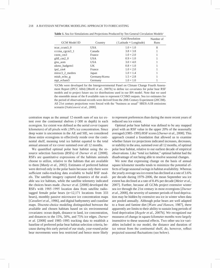
Table 1. Sea Ice Simulations and Projections Produced by Ten General Circulation Modelsa
GCM Model ID CountryGrid Resolution
( latitude ´ longitude)Number of
Runs
ncar_ccsm3_0 USA 1.0 ´ 1.0 8cccma_cgcm3_1 Canada 3.8 ´ 3.8 1cnrm_cm3 France 1.0 ´ 2.0 1gfdl_cm2_0 USA 0.9 ´ 1.0 1giss_aom USA 3.0 ´ 4.0 1ukmo_hadgem1 Uk 0.8 ´ 1.0 1ipsl_cm4 France 1.0 ´ 2.0 1miroc3_2_medres Japan 1.0 ´ 1.4 1miub_echo_g Germany/korea 1.5 ´ 2.8 1mpi_echam5 Germany 1.0 ´ 1.0 1aGCMs were developed for the Intergovernmental Panel on Climate Change Fourth Assess-ment Report (IPCC AR4) [Meehl et al., 2007b] to define ice covariates for polar bear RSF models and to project future sea ice distributions used in our BN model. Note that we used the ensemble mean of the 8 available runs to represent CCSM3 outputs. Sea ice estimates for the period of observational records were derived from the 20th Century Experiment (20C3M). All 21st century projections were forced with the “business as usual” SRES-A1B emissions scenario [Nakićenović et al., 2000].
AMSTRUP ET Al. 219
2.3.2. Seasonal habitat availability. Recognizing the po-tential importance of the seasonal separation of sea ice cover from preferred continental shelf foraging areas, and duration of such separation, we determined the number of ice-free months over the continental shelf and the average shelf- to-ice distance in both the observed and GCM-projected ice concentration maps. An ice-free month occurred in an ecore-gion when <50% of the shelf area was covered by sea ice of ≥50% concentration. Shelf ice distance was the mean distance from every shelf pixel in a polar basin ecoregion to the nearest ice-covered pixel (>50% concentration) dur-ing the month of minimum ice extent. This described how far polar bears occupying sea ice habitats would be from their preferred continental shelf foraging areas. The average shelf-to-ice distance was not calculated for the SIE and AE because we considered those ecoregions to be composed en-tirely of shelf waters.
2.4. Bayesian Network Population Stressor Model
A Bayesian network is a graphical model that represents a set of variables (nodes) linked by probabilities [Neopolitan, 2003; McCann et al., 2006]. Nodes can represent correlates or causal variables that affect some outcome of interest, and links define which specific variables directly affect which other specific variables. BNs can combine expert knowl-edge and empirical data into the same modeling structure. Crafting a BN augments understanding of relationships and sensitivities among the elements of a causal web and pro-vides insights into the workings of the system that otherwise would not have been evident. BNs have become an accepted and popular modeling tool in many fields [Pourret et al., 2008] including ecological and environmental sciences [e.g., Aalders, 2008; Uusitalo, 2007]. Each node in a BN model typically has two or more mutually exclusive states, the probabilities of which sum to one. Prior probabilities are dis-tributed as discontinuous Dirichlet functions in the form of D(x) = lim
m®¥ lim
n®¥ cos2n(m!px), which is a multivariate, n state
generalization of the two-state Beta distribution with state probabilities being continuous within [0,1]. BN nodes can represent categorical, ordinal, or continuous variable states or constant (scalar) values and typically have an associated probability table that describes either prior (unconditional) probabilities of each state for input nodes or conditional probabilities of each state for nodes that directly depend on other nodes (see Marcot et al. [2006] for a description of the underlying statistics). States S of output nodes contain posterior probabilities that are calculated conditional upon nodes H that directly affect them, using Bayes theorem, as P(S | H) = [P(H |S)P(S )/P(H )] (see Jensen [2001] and Mar-cot [2006] for further explanation of the statistical basis of
BNs). BNs are “solved” by specifying the values of input nodes and having the model calculate posterior probabilities of the output node(s) through “Bayesian learning” [Jensen, 2001]. BNs are useful for modeling systems where empiri-cal data are lacking, but variable interactions and their un-certainties can be depicted based on expert judgment [Das, 2000]. They are also particularly useful in efforts to synthe-size large amounts of divergent quantitative and qualitative information to answer “what if” kinds of questions.
Developing a BN model entails depicting the “causal web” of interacting variables [Marcot et al., 2006] in an influence diagram, assigning states to each node, and assigning prob-abilities to each node that define the conditions under which each state could occur. We used the modeling shell Netica® (Norsys, Inc.) and followed guidelines for developing BN models developed by Jensen [2001], Cain [2001], and Mar-cot et al. [2006].
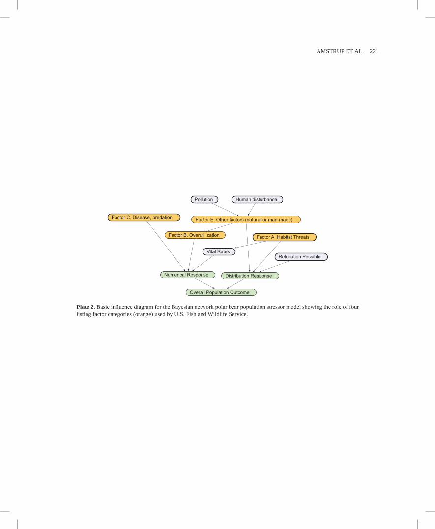
Our BN stressor model was based on the knowledge of one polar bear expert (S. Amstrup), who established the model structure and probability tables according to expected influences among variables. B. Marcot served as a “knowl-edge engineer” and provided guidance to help structure the expert’s knowledge into an appropriate BN format. Amstrup compiled an initial list of ecological correlates which were organized into an influence diagram (Plate 2). With discus-sion and questioning, Marcot guided Amstrup through sev-eral stages to a final model structure.
The BN model structure was divided into three kinds of nodes: (1) input nodes were anthropogenic stressors or environmental variables, states of input nodes were parameterized with unconditional probabilities; (2) sum-mary nodes, sometimes called latent variables [e.g., Bollen, 1989], collect and summarize effects of multiple input nodes, states of these were parameterized with con-ditional probability tables; and (3) output nodes that rep-resented numerical, distribution, and overall population responses to the suite of inputs. Probabilities of the vari-ous states of output nodes are derived through Bayesian learning. We developed the model structure in an iterative fashion adding variables for which we could hypothesize important roles. Published as well as unpublished informa-tion on how polar bears respond to changes in sea ice al-lowed us to parameterize the model to ensure it responded to particular input conditions in ways that paralleled re-sponses of polar bear populations that have been observed or for which there are strong prevailing hypotheses among polar bear biologists worldwide.
To assure our outcomes were relevant to the question whether to list polar bears as a threatened species, we designed the summary nodes in the BN model to include four of the five major listing factors used to determine a species’
220 A BAyESIAN NETWORk MODElING APPROACh TO FORECASTING
status according to the Endangered Species Act [U.S. Fish and Wildlife Service, 2007]. We included summary nodes for factor A, habitat threats; factor B, overutilization; factor C, disease and predation; and factor E, other natural or man-made factors. We did not include factor D, inadequacy of existing regulatory mechanisms, because our model focused on ecosystem effects; however, regulatory aspects could be seamlessly added at a future time.
2.5. Parameterizing the Bayesian Network Model
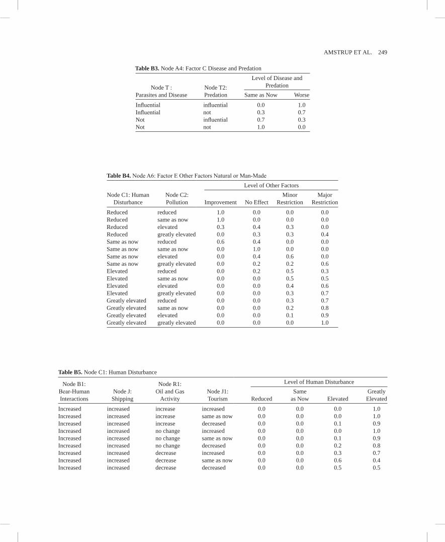
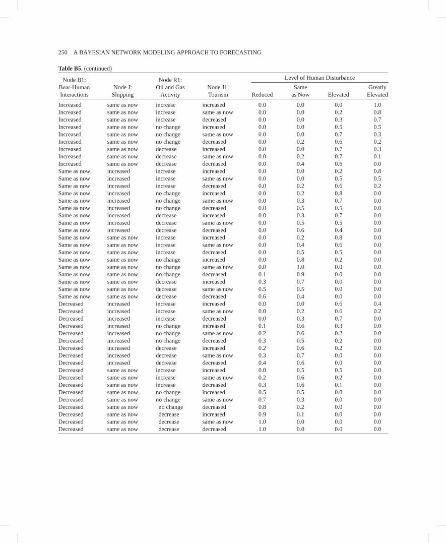
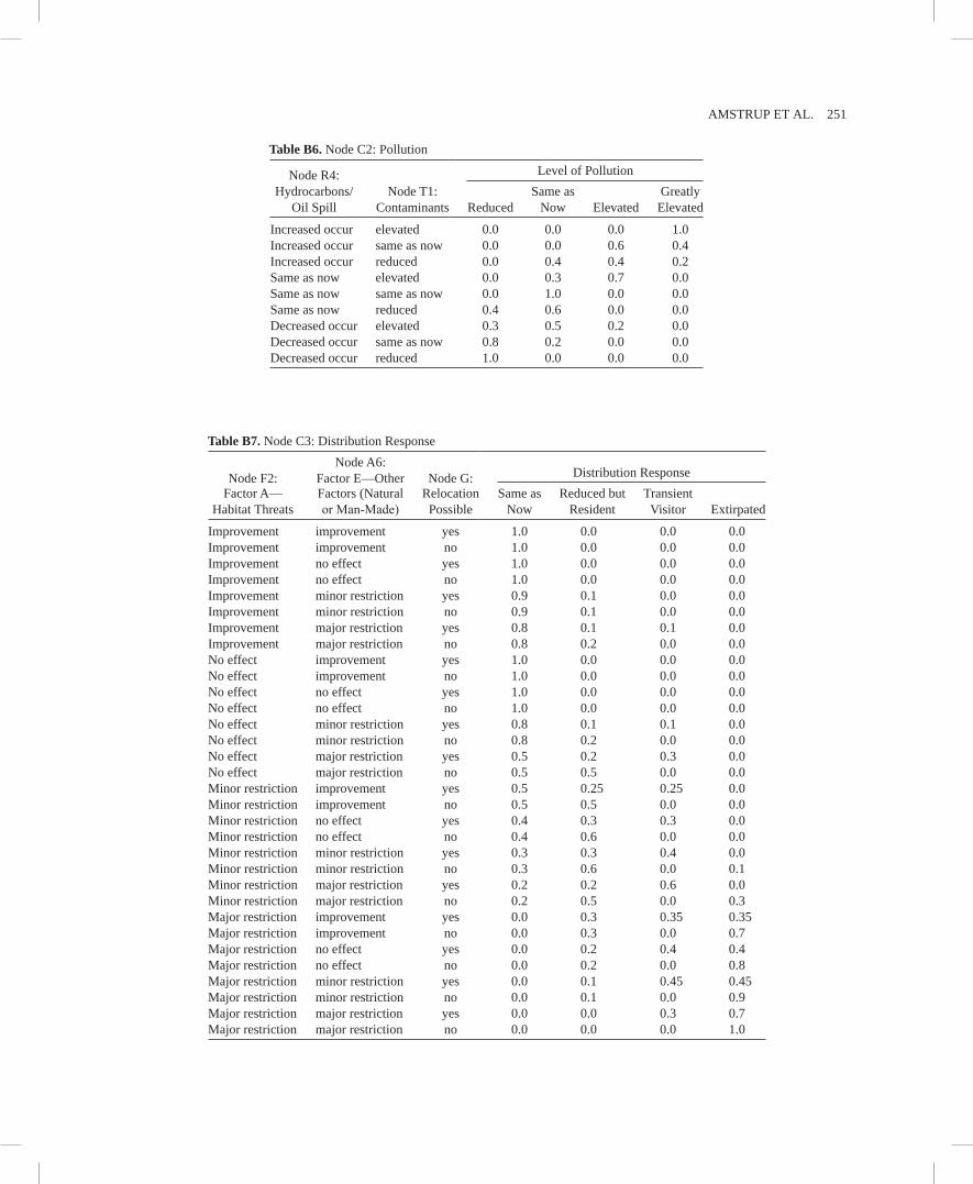
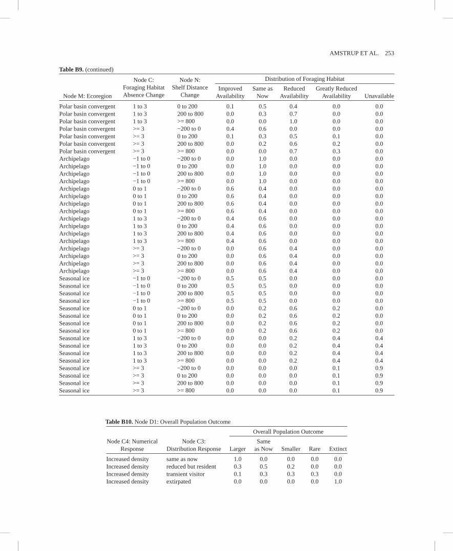
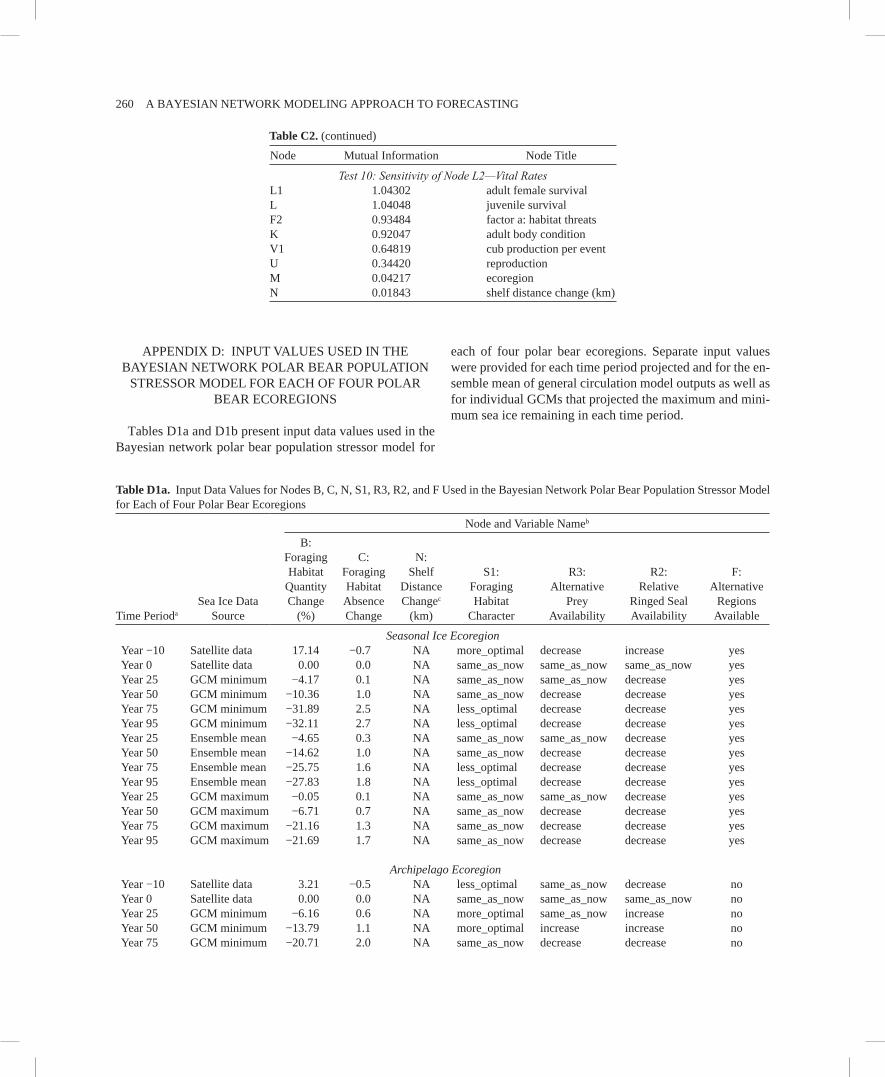
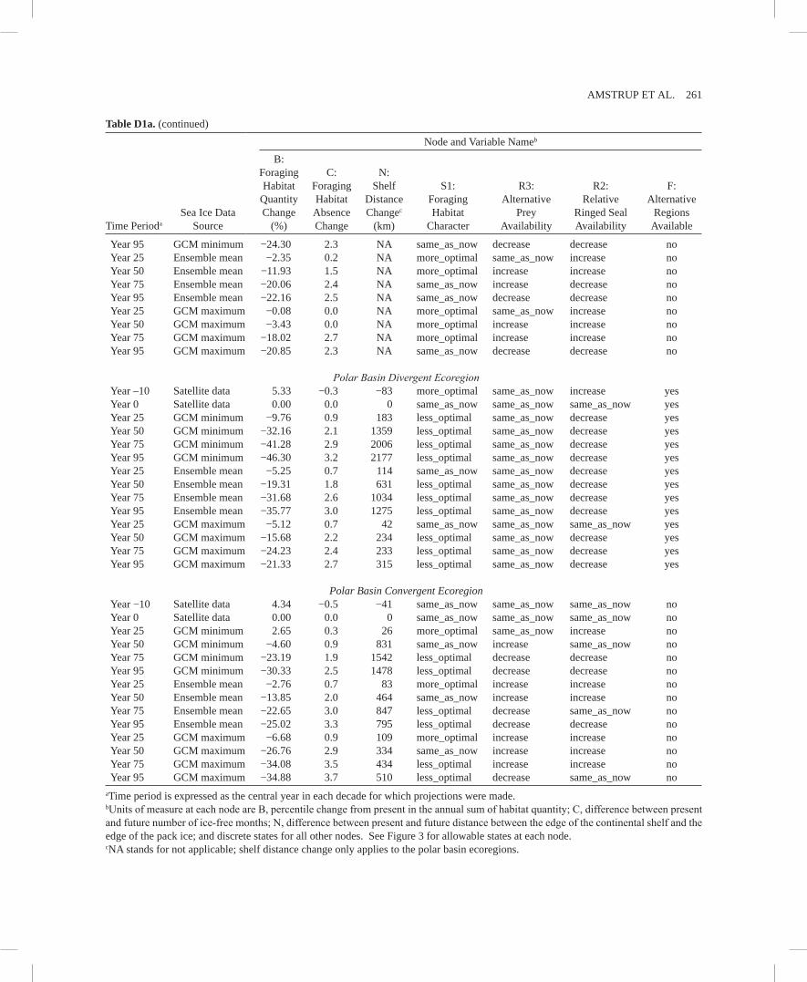
We averaged the sea ice parameters for each GCM over decadal periods to generate metrics that were less sensitive to the intrinsic variability of GCM projections that occurs at annual timescales. The BN model was applied to each of the four ecoregions at six decadal time periods: 1985–1995, 1996–2006, 2020–2029, 2045–2054, 2070–2079, and 2090–2099. For convenience, we hereinafter refer to these six time periods, in relation to the present, as years −10, 0, 25, 50, 75, and 95. Analyses included observed habitat con-ditions from the satellite passive microwave data for years −10 and 0 and future habitat conditions projected by GCM ice projections for future years. To capture the full range of uncertainty in GCM outputs, we solved the BN model using sea ice parameters from the (1) GCM multimodel (ensem-ble) means, (2) GCM that projected the minimum ice extent, and (3) GCM that projected the maximum ice extent, for each ecoregion in each time period. Inputs other than sea ice features included various categories of anthropogenic stres-sors [Barrett, 1981] such as harvest, pollution, oil and gas development, shipping, and direct bear-human interactions. Inputs also included other environmental factors that could affect polar bear populations such as availability of primary and alternate prey and foraging areas and occurrence of par-asites, disease, and predation [Ramsay and Stirling, 1984]. Whereas the ice habitat factors were entered into the BN model as ranges of values (e.g., ice retreat of 0–200 or 200–800 km beyond current measures), other potential stressors were included as ordinal or qualitative categories (Tables D1a and D1b).
Because we were interested in forecasting changes from cur-rent conditions, states of each node were expressed categori-cally as “compared to now.” That is, an outcome state could represent a condition similar to present, better than present, or worse than present. Here, now or year “0” means the 1996–2006 period when referring to observations and 2000–2009 when referring to sea ice model projections. Before the BN model was run, we specified the states for each input node that seemed most plausible (Tables D1a and D1b).
States of environmental correlates were established under each combination of time step, ecoregion, and GCM model
outputs. We ensured that input conditions matched the cur-rent understanding of polar bear ecology and parameterized the conditional probability tables to assure that node struc-tures were specified in accordance with available polar bear data or expert understanding of data. We checked the valid-ity of the model parameterization by testing whether the BN model responded to particular input conditions in ways that paralleled responses of polar bear populations to conditions that have been observed.
When the model is run, it calculates posterior probabilities of outcomes by applying standard Bayesian learning to the values assigned to each input variable. The relative influ-ence of each input node, in terms of inherent model sensi-tivity structure, is determined by the values assigned in the conditional probability tables that underlie each summary or output node in the network. One input variable can be given greater influence than another if the result of a change in the first variable is thought to have a greater influence on the outcome states of the summary or output node than the second, and if the conditional probabilities are assigned ac-cordingly. For example, it may be thought that the temporal absence of sea ice from the continental shelf is more impor-tant to the availability of foraging habitat than is the distance to which the ice retreats while it is absent. If data or pro-jections suggest both measurements change in parallel, then temporal absence would have the greater final influence. If, however, data or projections show there is a greater change in distance than in time of absence, then distance may have the greatest contribution to posterior (outcome) probabilities even though its weight in the conditional probability table might be lower than temporal absence.
We used three different methods to arrive at final model structure: (1) sensitivity analyses of subparts of the model, (2) solving the model backward by specifying outcome states and evaluating if the most likely input states that were returned were plausible according to what we know about polar bears now, and (3) running the model (and subparts) forward to ascertain if the summary and output nodes re-sponded as expected given the states of the input nodes. Our goals were to ensure that input conditions matched the cur-rent understanding of polar bear ecology and that the model responded to particular input conditions in ways that paral-leled observed responses of polar bear populations.
As fully specified, the BN model consisted of 38 nodes, 44 links, and 1667 conditional probability values specified by the modelers (Plate 3 and Appendices A and B). The model was solved for each combination of four ecoregions, six time periods, and three future GCM scenarios (ensemble mean, maximum, and minimum).
The input data to run each combination were specified by summarizing the respective GCM-derived habitat variables
AMSTRUP ET Al. 221
Plate 2. Basic influence diagram for the Bayesian network polar bear population stressor model showing the role of four listing factor categories (orange) used by U.S. Fish and Wildlife Service.
Plat
e 3
AMSTRUP ET Al. 223
and the professional judgment of polar bear expert S. Amstrup (Tables D1a and D1b). Because BN models combine expert judgment and interpretation with quantitative and qualita-tive empirical information, inputs from multiple experts are sometimes used to structure and parameterize a “final” model. Because the model presented was parameterized with the judg-ment of only one polar bear expert, it should be viewed as a first-generation version. Accordingly, it will be refined through formally developed processes (see section 4) at a future time.
2.6. Output States of the Bayesian Network Model
The final outcomes of BN model runs were statements of relative probabilities that the population in each ecoregion would be larger than now, same as now, smaller than now, rare, or extinct. Responses of polar bears to projected habitat changes and other potential stressors could affect polar bear distribution or polar bear numbers independently in some cases, or they could affect both distribution and numbers si-multaneously. Principal results of the BN model are levels of relative probabilities for the potential states at output nodes. In the polar bear BN population stressor model, outcomes of greatest interest were (1) those related to listing factors used by the FWS, (2) the distribution responses, (3) numerical responses, and (4) the overall population response.
We defined our output nodes (shown in Plate 3) in such a way that their possible states could be assessed empirically through future field observations. Potential states at the three principal output nodes are described below.
2.6.1. Node C4: Numerical response. This node represents the anticipated numerical response of polar bears in an eco-region based upon the sum total of the identified factors which are likely to have affected numbers of polar bears in each ecoregion:
· increased density, polar bear density detectable as significantly greater than that at year 0, where density can be expressed in terms of number of polar bears per unit area of optimal habitat (thus expressing “eco-logical density”) or of total (optimal plus suboptimal) habitat (thus expressing “crude density”);
· same as now, equivalent to the density at year 0; · reduced density, polar bear density less than that at year
0 but greater than one half of the density at year 0; · rare, polar bear density less than half of that at year 0; · absent, polar bears are not demonstrably present.
2.6.2. Node C3: Distribution response. Distribution re-fers here to the functional response of polar bears (namely, movement and spatial redistribution of bears) to changing conditions:
· same as now, polar bear distribution equivalent to that at year 0;
· reduced but resident, bears would still occur in the area but their spatial distribution would be more lim-ited than at year 0;
· transient visitors, changing conditions would season-ally limit distribution of polar bears;
· extirpated, complete or effective year-round dearth of polar bears in the area.
2.6.3. Node D1: Overall population outcome. Overall population outcome refers to the collective influence of both numerical response (node C4) and distribution response (node C3). It incorporates the full suite of effects from all anthropogenic stressors, natural disturbances, and environ-mental conditions on the expected occurrence and levels of polar bear populations in the ecoregion. Overall population outcome states were defined as follows:
· larger, polar bear populations have a numerical re-sponse greater than at present (year 0) and a distribu-tion response at least the same as at present;
· same as now, polar bear populations numerically and distributionally indistinguishable from present;
· smaller, polar bears at a reduced density and dis-tributed the same as at present or density same as at present but occur as transient visitors;
· rare, polar bears are numerically difficult to detect and have a distribution response same as at present, or oc-cur as small numbers of transient visitors;
· extinct, polar bears are numerically absent or distribu-tionally extirpated.
Here, the “extinct” state refers to conditions of (1) com-plete absence of the species (N=0) from an ecoregion; or (2) numbers and distributions below a “quasi-extinction” level, that refers to a nonzero population level at or below which the population is near extinction [Ginzburg et al., 1982; Ot-way et al., 2004]; or (3) functional extinction, that refers to being so scarce as to be near extinction and contributing negligibly to ecosystem processes [Sekercioglu et al., 2004; McConkey and Drake, 2006].
Plate 3. (Opposite) Full Bayesian network population stressor model developed to forecast polar bear population outcomes in the 21st century. Values shown in the bottom of nodes B, N, and C represent expected values +/- 1 standard deviation which are automatically calculated and displayed by the Netica® modeling shell for continuous nodes with defined state values, based on Gaussian distributions.
224 A BAyESIAN NETWORk MODElING APPROACh TO FORECASTING
Outcomes from the BN model are expressions of probability that each outcome state will occur (e.g., X% extinct, y% rare, and Z% smaller). It is important here to understand that these probability values are provided without error bars and should not, in themselves, be interpreted as absolute measures of the certainty of any particular outcome. Rather, probabilities of outcome states of the model should be viewed in terms of their general direction and overall magnitudes. When predic-tions result in high probability of one outcome state and low or zero probabilities of all other states, there is low overall uncertainty of predicted results. When projected probabilities of various states are more equally distributed or when two or more states have large probability, there is greater uncertainty in the outcome. In these cases, careful consideration should be given to large probabilities representing particular states even if those probabilities are not the largest.
2.7. Sensitivity of the Bayesian Network Model
knowledge of polar bears, their dependence on sea ice, the ways in which sea ice changes have been observed to affect polar bears, and professional judgment regarding how ecological and human factors may differ if sea ice changes occur as projected were used to populate the conditional probability tables in the BN model. Because our model in-corporated the professional judgment of only one polar bear expert, it is reasonable to ask how robust the results might be to input probabilities which could vary among other experts. It also is appropriate to ask whether it is likely that future sea ice change, to which model outcomes are very sensi-tive, could fall into ranges that would result in qualitatively different outcomes than our BN model projects. Finally, it is appropriate to ask the extent to which model outcomes may be altered by active management of the states of nodes which represent variables humans could control.
We addressed questions about the ability of changes in human activities to alter the BN output states by fixing in-puts humans could control and examining differences in the overall outcomes. We evaluated the extent to which sea ice projections would have to differ to make qualitative dif-ferences in outcomes by holding all non-ice variables at uniform priors and allowing ice variables only to vary at future time steps. Comparing those results to the range of ice conditions projected by our GCMs provided a sense of just how much the realized future ice conditions would have to vary from those projected to make a difference in popu-lation outcomes. Finally, although we cannot second guess how other polar bear experts may recommend parameteriz-ing and structuring a BN model, comparison of model runs with preset values provides some sense of how much dif-ferently the model would have to be parameterized to pro-
vide qualitatively different outcome patterns than those we obtained.
We ran overall sensitivity analyses to determine the de-gree to which each input and summary variable influenced the outcome variables. For discrete and categorical variables, sensitivity was calculated in the modeling shell Netica® as the degree of entropy reduction (reduction in the disorder or variation) at one node relative to the information represented in other nodes of the model. That is, the sensitivity tests indi-cate how much of the variation in the node in question is ex-plained by each of the other nodes considered. The degree of entropy reduction, I, is the expected reduction in mutual infor-mation of an output variable Q, with q states, due to a finding of an input variable F, with f states. For discrete variables, I is measured in terms of information bits and is calculated as
I H Q H Q F q fP q f log2 P q f
P q P f
where H(Q) is the entropy of Q before new findings are ap-plied to input node F and H(Q|F) is the entropy of Q after new findings are applied to F. In Netica®, entropy reduction is also termed mutual information.
For continuous variables, sensitivity is calculated as var-iance reduction VR, which is the expected reduction in vari-ation, V(Q), of the expected real value of the output variable Q due to the value of input variable F, and is calculated as
VR V Q V Q F
where
V Q q P q Xq E Q 2
V Q F q P q f Xq E Q f 2
E Q q P q Xq
and where Xq is the numeric real value corresponding to state q, E(Q) is the expected real value of Q before new findings are applied, E(Q|F) is the expected real value of Q after new findings f are applied to F, and V(Q) is the variance in the real value of Q before any new findings [Marcot et al., 2006].
3. RESUlTS
3.1. Bayesian Network Model Outcomes
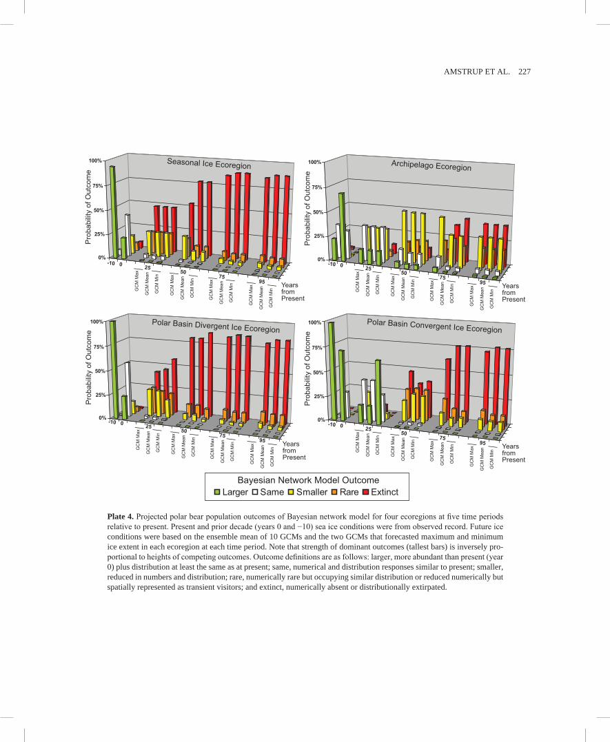
The most probable BN model outcome, for both the SIE and PBDE, was “extinct” (Table 2 and Plate 4). In all but
AMSTRUP ET Al. 225
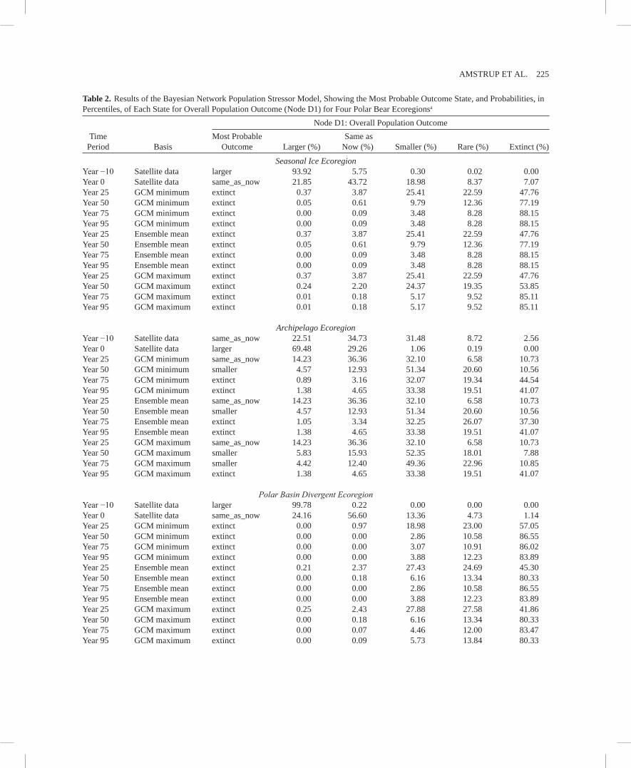
Table 2. Results of the Bayesian Network Population Stressor Model, Showing the Most Probable Outcome State, and Probabilities, in Percentiles, of Each State for Overall Population Outcome (Node D1) for Four Polar Bear Ecoregionsa
Node D1: Overall Population OutcomeTime
Period BasisMost Probable
Outcome larger (%) Same as Now (%) Smaller (%) Rare (%) Extinct (%)
the earliest time periods, we forecasted low probabilities for all other outcome states in these two ecoregions. The low probability afforded to outcome states other than extinct suggested a clear trend in these ecoregions toward prob-able extirpation by mid century. Forecasts were less severe in other ecoregions. At year 50, probability of the “extinct” state was only 8–10% in the AE. At all time steps in the AE, and at year 50 in the PBCE, considerable probability fell into outcome states other than extinct (Table 2 and Plate 4). The distribution of probabilities for the states of overall population outcome suggests polar bears could persist in all ecoregions through the early part of the century, through mid century in the PBCE and through the end of the century in the AE (Table 2 and Plate 4).
Future conditions affected node C3, polar bear distribution, more than they affected node C4, polar bear numbers. “Ex-tirpated” was the most probable outcome at mid century for node C3 in the PBDE and SIE. The most probable outcome in these ecoregions for node C4, however, was reduced den-sity [see Amstrup et al., 2007]. This probably reflects the high relative certainty that areas where ice is absent for too long will not support many bears, and the relative uncertainty re-garding how population dynamics features may change while the sea ice is retreating. Modeled future polar bear distribu-tions were driven by the FWS listing factor “Habitat Threats” (node F2, Table 3), as well as by node D, habitat distribu-tion. Distribution and availability of habitat, especially in the
SIE and PBDE (Table 3) appear to be the most salient threats to polar bears. We also assumed that deteriorating sea ice would be accompanied by worsening conditions listed un-der FWS listing factors C, disease and predation, etc., and E, other natural or man-made factors (nodes A4 and A6) (Table 4). We included year 25 in our projections to help provide context for mid century projections and beyond and to help understand the transition from current to future conditions. It is important to emphasize, however, that polar bears have a long life span. Many individuals alive now could still be alive during the decade of 2020–2029. hence, projecting changes between now and then incorporates the uncertainty of trade-offs between functional and numerical responses, as well as the greater uncertainties in sea ice status in the nearer term.
3.2. Sensitivity Structure of the Bayesian Network Model
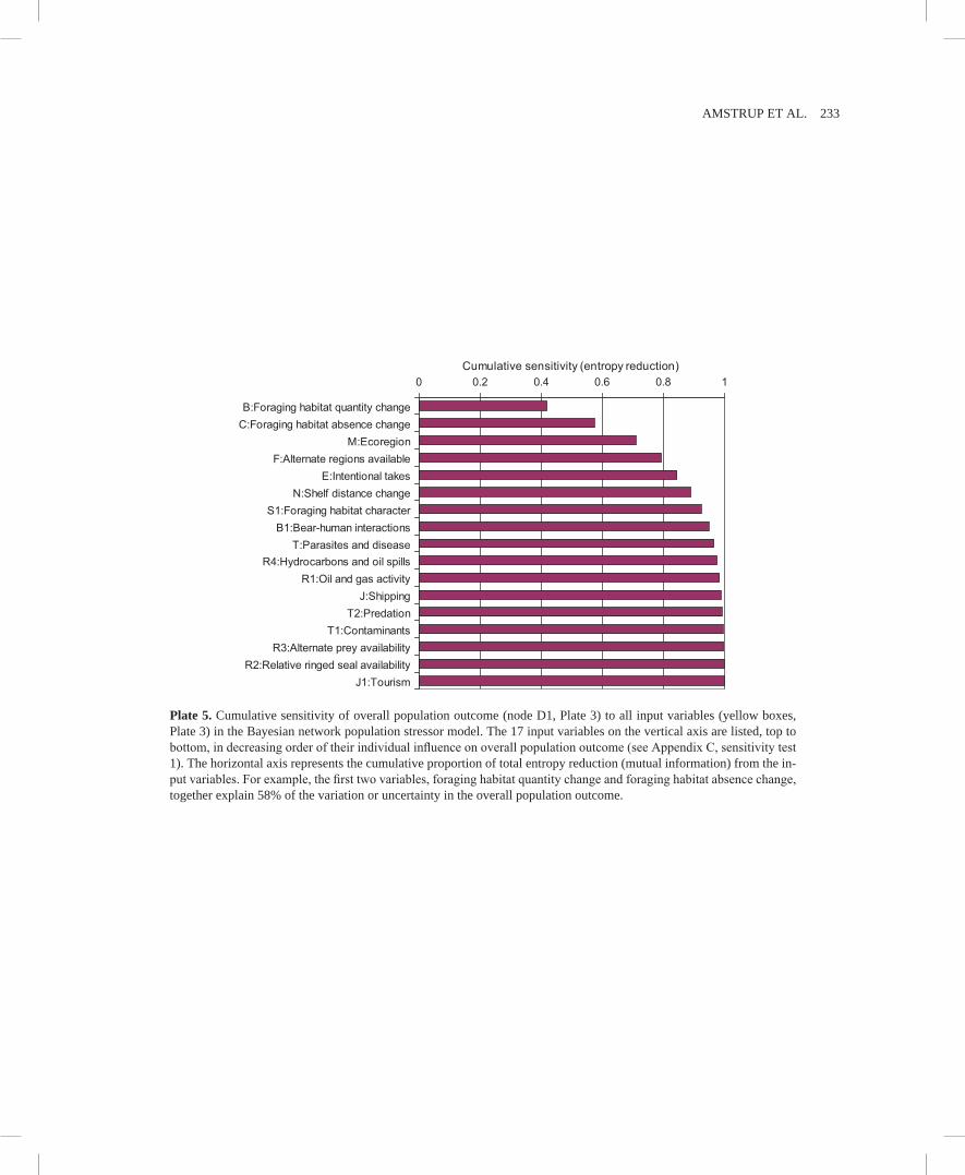
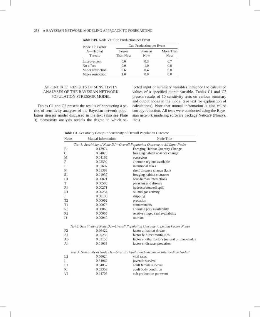
We conducted 10 tests on the BN population stressor model to determine its sensitivity structure (Appendix C). The BN model was well balanced in that sensitivity of over-all population outcome (node D1, sensitivity test 1) was not dominated by a single or small group of input variables. Considering that “ecoregion” and “availability of alternate regions” are in essence habitat variables, 6 of the top 7 vari-ables explaining overall outcome were sea ice related and together explained 87% of the variation in overall popula-tion outcome (node D1, Appendix C and Plate 5).
AMSTRUP ET Al. 227
Plate 4. Projected polar bear population outcomes of Bayesian network model for four ecoregions at five time periods relative to present. Present and prior decade (years 0 and −10) sea ice conditions were from observed record. Future ice conditions were based on the ensemble mean of 10 GCMs and the two GCMs that forecasted maximum and minimum ice extent in each ecoregion at each time period. Note that strength of dominant outcomes (tallest bars) is inversely pro-portional to heights of competing outcomes. Outcome definitions are as follows: larger, more abundant than present (year 0) plus distribution at least the same as at present; same, numerical and distribution responses similar to present; smaller, reduced in numbers and distribution; rare, numerically rare but occupying similar distribution or reduced numerically but spatially represented as transient visitors; and extinct, numerically absent or distributionally extirpated.
228 A BAyESIAN NETWORk MODElING APPROACh TO FORECASTING
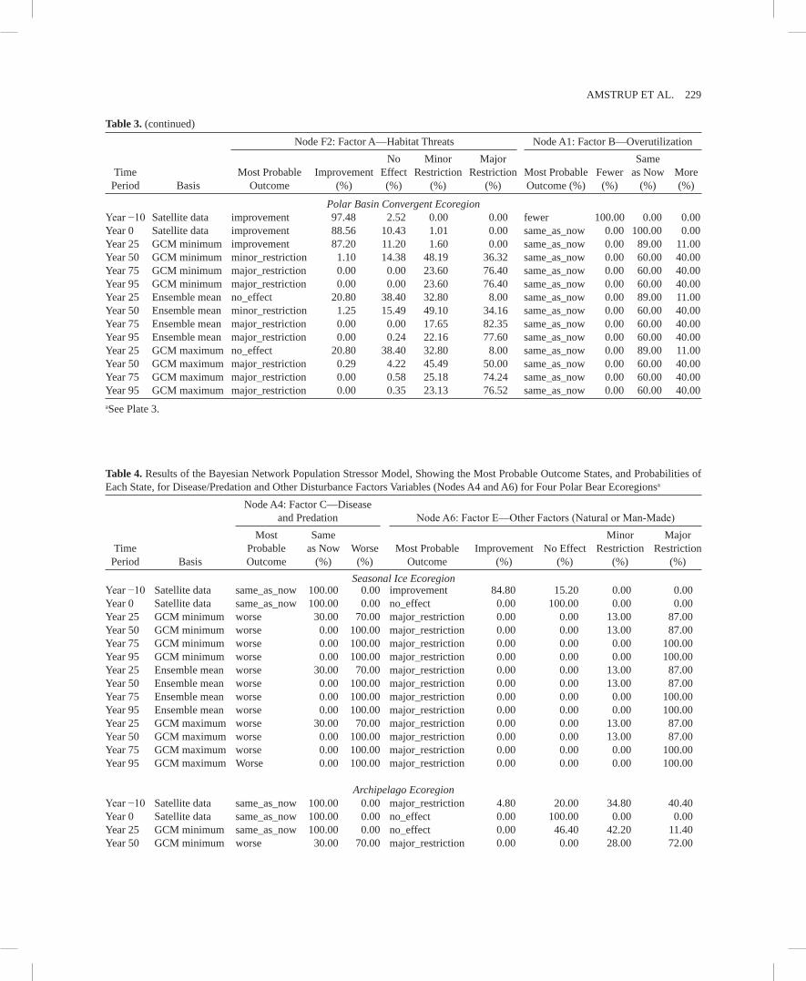
Table 3. Results of the Bayesian Network Population Stressor Model, Showing the Most Probable Outcome States, and Probabilities of Each State, in Percentiles, for habitat Threats and Direct Mortalities Summary Variables (Nodes F2 and A1) for Four Polar Bear Ecoregionsa
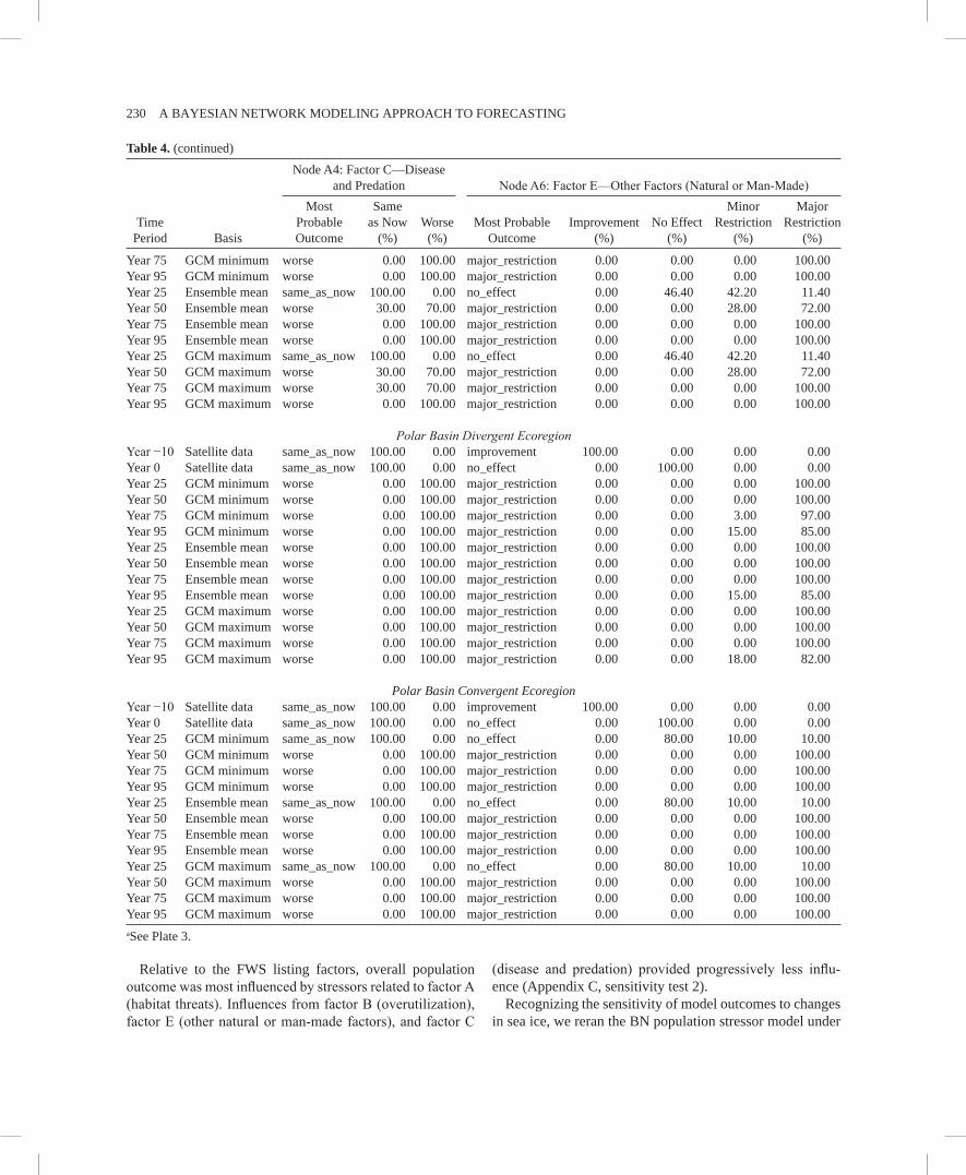
Table 4. Results of the Bayesian Network Population Stressor Model, Showing the Most Probable Outcome States, and Probabilities of Each State, for Disease/Predation and Other Disturbance Factors Variables (Nodes A4 and A6) for Four Polar Bear Ecoregionsa
Node A4: Factor C—Disease and Predation Node A6: Factor E—Other Factors (Natural or Man-Made)
Relative to the FWS listing factors, overall population outcome was most influenced by stressors related to factor A (habitat threats). Influences from factor B (overutilization), factor E (other natural or man-made factors), and factor C
(disease and predation) provided progressively less influ-ence (Appendix C, sensitivity test 2).
Recognizing the sensitivity of model outcomes to changes in sea ice, we reran the BN population stressor model under
AMSTRUP ET Al. 231
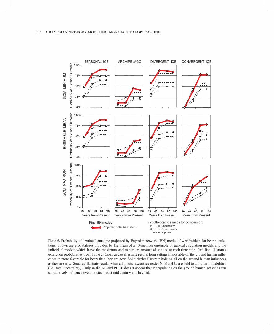
two sets of fixed conditions to determine whether manage-ment of human activities on the ground might be able to alter sea ice–driven outcomes. In these “influence runs” we set the states for all nodes over which humans might be able to exert control (e.g., harvest, contaminants, oil, and gas devel-opment) first to “same as now,” and then to “improved con-ditions.” After doing so, projected probabilities of extinction were lower at every time step (Plate 6). At and beyond mid century, extinction was still the most probable outcome in the PBDE and SIE. however, extinction did not become the most probable outcome in the PBDE and SIE until mid cen-tury. And in the SIE, with model runs based on GCMs retain-ing the maximum sea ice, extinction, as the most probable outcome, was avoided until year 75. Recall that extinction was the most probable outcome in these ecoregions at year 25 in the original model runs. In contrast, results of these influence runs suggested that on the ground management of human activities could improve the fate of polar bears in the AE and PBCE through the latter part of the century (Plate 6). In summary, for our 50-year foreseeable future, it appeared that management of localized human activities could benefit polar bears in the PBCE and especially in the AE but was likely to have little qualitative effect on the future of polar bears in the PBDE and SIE if sea ice continues to decline as projected.
To examine how much different, than projected, future sea ice would need to be to cause a qualitative change in our overall outcomes, we composed another influence run in which we set the values for all non-ice inputs to uniform prior probabilities. That is, we assumed complete uncertainty with regard to future food availability, oil and gas activity, con-taminants, disease, etc. Then, we ran the model to determine how changes in the sea ice states alone, specified by our en-semble of GCMs, would affect our outcomes. This exercise illustrated that in order to obtain any qualitative change in the probability of extinction in any of the ecoregions, sea ice projections would need to leave more sea ice, at all future time steps, than even the maximum-ice GCM projection we used (Plate 6).
4. DISCUSSION
4.1. Uncertainty
Analyses in this paper contain four main categories of uncertainty: (1) uncertainty in our understandings of the biological, ecological, and climatological systems; (2) un-certainty in the representation of those understandings in models and statistical descriptions; (3) uncertainty in pre-dictions of species abundance and distribution, and (4) uncertainty in model credibility, acceptability, and appropri-
ateness of model structure. All of these can influence model predictions. Uncertainty in our understanding of complex ecosystems is virtually inevitable. We have, however, dealt with this as well as possible by incorporating a broad sweep of available information regarding polar bears and their en-vironment. how to best represent our understanding of the system in models, the second source of uncertainty, can be structured in various ways. here, we captured and repre-sented expert understanding of polar bear habitats and popu-lations in a manner that can be reviewed, tested, verified, calibrated, and amended as appropriate. We have attempted to open the “black box” so to speak and to fully expose all formulas and probabilities. We also used sensitivity testing to understand the dynamics of BN model predictions [John-son and Gillingham, 2004] (Appendix C). After BN models of this type are modified through peer review or revised by incorporating the knowledge from more than one expert into the model parameterization, any variation in resulting mod-els can represent the divergence (or convergence) of exper-tise and judgment among multiple specialists.
Also included in the second category of uncertainty are those associated with statistical estimation of parameters, including measurement and random errors. The sea ice pa-rameters we used in our polar bear models were derived from GCM outputs that possess their own wide margins of uncertainty [DeWeaver, 2007]. hence, the magnitude and distribution of errors associated with our sea ice parameters were unknown. To compensate for these unknowns, we ac-commodated a broad range of sea ice uncertainties by ana-lyzing the 10-member ensemble GCM mean, as well as the minimum and maximum GCM ice forecasts. In the case of polar bear population estimates, many are known so poorly that the best we have are educated guesses. Pooling sub-populations where numbers are merely guesses with those where precise estimates are available, to gain a range-wide perspective, prevents meaningful calculation and incorpo-ration of specific error terms. We recognize that difficulty, but because our projections are expressed in the context of a comparison to present conditions, we largely avoid the issue. That is, whatever the population size is now, the future size is expressed relative to that and all errors are carried forward.
The third category, uncertainty in predictions of species abundance and distribution can be subject to errors because of spatial autocorrelation, dispersal and movement of organ-isms, and biotic and environmental interactions [Guisan et al., 2006]. We addressed these error sources by deriving es-timates of ice habitat area separately for each ecoregion from the GCM models because sea ice formation, melt, and advec-tion occur differently in each ecoregion. The BN population stressor model accounted explicitly for potential movement
232 A BAyESIAN NETWORk MODElING APPROACh TO FORECASTING
of polar bears (e.g., availability of alternative regions) and for biotic and environmental interactions (as expressed in the conditional probability tables; see Appendix B). The spread of probabilities among the BN outcome states, reflect the combinations of uncertainties in states across all other variables, as reflected in each of their conditional probability tables (Appendix B). This spread carries important informa-tion for the decision maker who needs to weigh alternative outcomes in a risk assessment (see below).
Finally, uncertainty in model predictions entails address-ing model credibility, acceptability, and appropriateness of the model structure. We made every effort to ensure that the model structure was appropriate and credible and that the in-puts (Tables D1a and D1b) and conditional probability tables (Appendix B) were parameterized according to best avail-able knowledge of polar bears and their environment. We explored the logic and structure of our BN model through sensitivity analyses, running the model backward from par-ticular states to ensure it returned the appropriate starting point, and performing particular “what if” experiments (e.g., by fixing values in some nodes and watching how values at other nodes respond). We are as confident as we can be at this point of development that our BN model is performing in a plausible manner and providing outcomes that can be useful in qualitatively forecasting the potential future status of polar bears.
Although this manuscript and the model it describes have been peer reviewed by additional polar bear experts, the model structure and parameterizations were based upon the judgments of only one expert. Therefore, additional criteria of model validation must be addressed through subsequent peer review of the model parameters and structure [Mar-cot et al., 1983; Marcot, 1990, 2006; Marcot et al., 2006]. This requirement means the model presented here should be viewed as a first-generation alpha level model [Marcot et al., 2006]. The next development steps have been described in detail by Marcot et al. [2006] and include peer review of the alpha model by other subject matter experts and con-sideration of their judgments regarding model parameteriza-tion; reconciliation of the peer reviews by the initial expert; updating the model to a beta level that incorporates the re-views; and testing the beta model for accuracy with exist-ing data (e.g., determining if it matches historic or current known conditions). Additional updating of the model can include incorporation of new data or analyses if available. Throughout this process, sensitivity testing is used to verify model performance and structure. This framework has been used successfully for developing a number of BN models of rare species of plants and animals [Marcot et al., 2001, 2006; Raphael et al., 2001; Marcot , 2006]. Model variants that may have emerged in this process would represent the
range of expert judgments and experiences (possibly veri-fied with new data), and this range could be important infor-mation for decision making.
Because these additional steps in development have not yet been completed, it is important to view probabilities of outcome states of our first-generation model in terms of their general direction and overall magnitudes rather than focusing on the exact numerical probabilities of the outcomes. When predictions result in high probability of one population outcome state and low or zero probabili-ties of all other states, there is low overall uncertainty of predicted results. When projected probabilities of various states are more equally distributed, however, careful con-sideration should be given to large probabilities represent-ing particular outcomes even if those probabilities are not the largest. Consistency of pattern among scenarios (e.g., different GCM runs) also is important to note. If the most probable outcome has a much higher probability than all of the other states and if the pattern across time frames and GCM models is consistent, confidence in that outcome pat-tern is high. If, on the other hand, probabilities are more uniformly spread among different states and if the pattern varies among scenarios, importance of the numerically most probable outcome should be tempered in view of the com-peting outcomes. This approach takes advantage of the in-formation available from the model while recognizing that it is still in development. It also conforms to the concept of viewing the model as a tool describing relative probabilis-tic relationships among major levels of population response under multiple stressors.
4.2. Bayesian Network Model Outcomes
In the BN model, for each scenario run, the spread of population outcome probabilities (or at least nonzero possi-bilities) represented how individual uncertainties propagate and compound across multiple stressors. Beyond year 50, “extinct” was the most probable overall outcome state for all polar bear ecoregions, except the AE (Plate 4 and Table 2). For the decade of 2020–2029, outcomes were intermediate between the present (year 0) and the foreseeable future (year 50) time frames. We projected that polar bear numbers in the AE and PBCE could remain the same as now through the earlier decade, becoming smaller by mid century. In the SIE and PBDE, polar bears appeared to be headed toward ex-tinction soon. however, probabilities they may persist in the PBDE and SIE were much higher at year 25 than at mid cen-tury (Plate 4). Although our BN model suggests polar bears are most likely to be absent from the PBDE and SIE by mid century, there is much uncertainty regarding when, between now and then, they might disappear from these ecoregions.
AMSTRUP ET Al. 233
Plate 5. Cumulative sensitivity of overall population outcome (node D1, Plate 3) to all input variables (yellow boxes, Plate 3) in the Bayesian network population stressor model. The 17 input variables on the vertical axis are listed, top to bottom, in decreasing order of their individual influence on overall population outcome (see Appendix C, sensitivity test 1). The horizontal axis represents the cumulative proportion of total entropy reduction (mutual information) from the in-put variables. For example, the first two variables, foraging habitat quantity change and foraging habitat absence change, together explain 58% of the variation or uncertainty in the overall population outcome.
234 A BAyESIAN NETWORk MODElING APPROACh TO FORECASTING
Plate 6. Probability of “extinct” outcome projected by Bayesian network (BN) model of worldwide polar bear popula-tions. Shown are probabilities provided by the mean of a 10-member ensemble of general circulation models and the individual models which leave the maximum and minimum amount of sea ice at each time stop. Red line illustrates extinction probabilities from Table 2. Open circles illustrate results from setting all possible on the ground human influ-ences to more favorable for bears than they are now. Solid circles illustrate holding all on the ground human influences as they are now. Squares illustrate results when all inputs, except ice nodes N, B and C, are held to uniform probabilities (i.e., total uncertainty). Only in the AE and PBCE does it appear that manipulating on the ground human activities can substantively influence overall outcomes at mid century and beyond.
AMSTRUP ET Al. 235
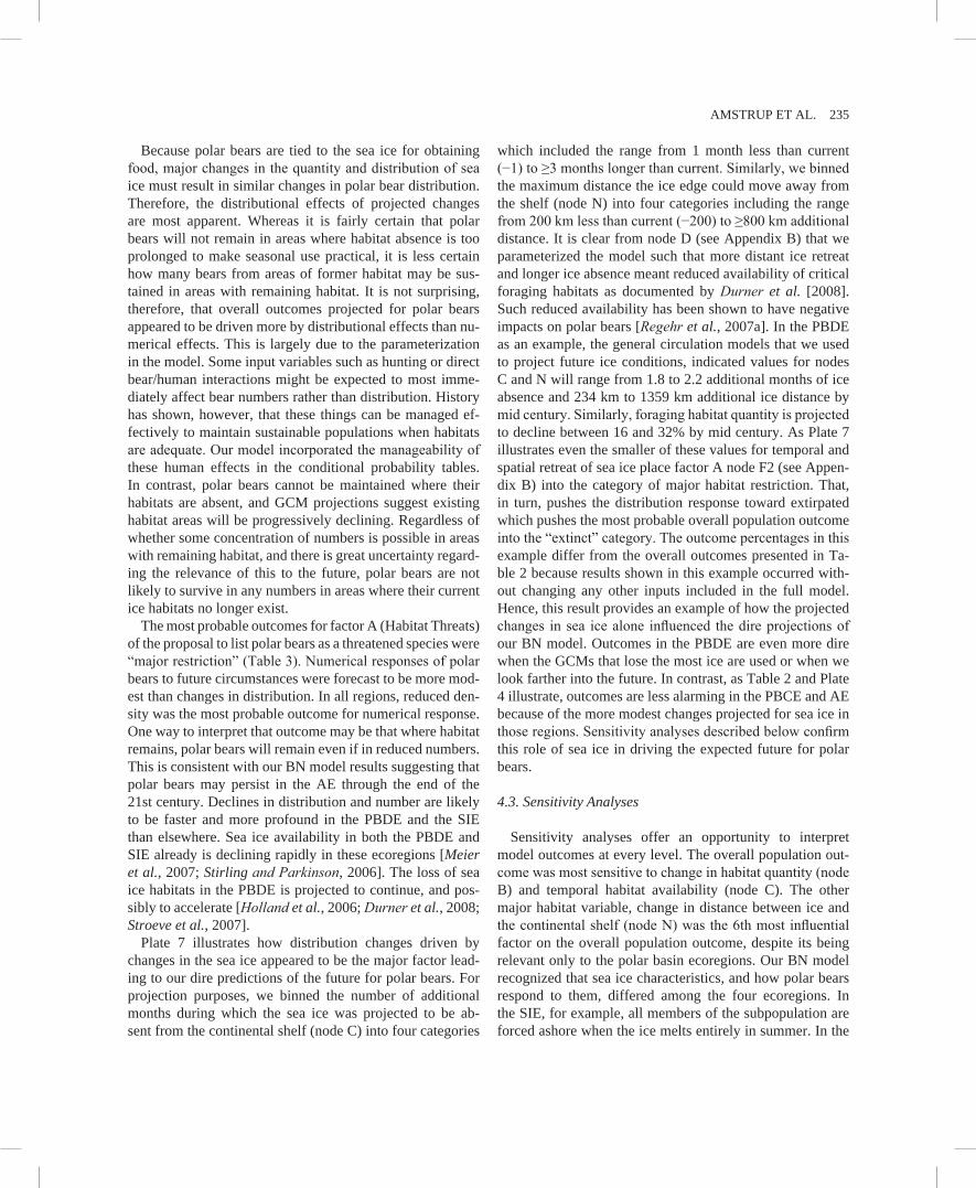
Because polar bears are tied to the sea ice for obtaining food, major changes in the quantity and distribution of sea ice must result in similar changes in polar bear distribution. Therefore, the distributional effects of projected changes are most apparent. Whereas it is fairly certain that polar bears will not remain in areas where habitat absence is too prolonged to make seasonal use practical, it is less certain how many bears from areas of former habitat may be sus-tained in areas with remaining habitat. It is not surprising, therefore, that overall outcomes projected for polar bears appeared to be driven more by distributional effects than nu-merical effects. This is largely due to the parameterization in the model. Some input variables such as hunting or direct bear/human interactions might be expected to most imme-diately affect bear numbers rather than distribution. history has shown, however, that these things can be managed ef-fectively to maintain sustainable populations when habitats are adequate. Our model incorporated the manageability of these human effects in the conditional probability tables. In contrast, polar bears cannot be maintained where their habitats are absent, and GCM projections suggest existing habitat areas will be progressively declining. Regardless of whether some concentration of numbers is possible in areas with remaining habitat, and there is great uncertainty regard-ing the relevance of this to the future, polar bears are not likely to survive in any numbers in areas where their current ice habitats no longer exist.
The most probable outcomes for factor A (habitat Threats) of the proposal to list polar bears as a threatened species were “major restriction” (Table 3). Numerical responses of polar bears to future circumstances were forecast to be more mod-est than changes in distribution. In all regions, reduced den-sity was the most probable outcome for numerical response. One way to interpret that outcome may be that where habitat remains, polar bears will remain even if in reduced numbers. This is consistent with our BN model results suggesting that polar bears may persist in the AE through the end of the 21st century. Declines in distribution and number are likely to be faster and more profound in the PBDE and the SIE than elsewhere. Sea ice availability in both the PBDE and SIE already is declining rapidly in these ecoregions [Meier et al., 2007; Stirling and Parkinson, 2006]. The loss of sea ice habitats in the PBDE is projected to continue, and pos-sibly to accelerate [Holland et al., 2006; Durner et al., 2008; Stroeve et al., 2007].
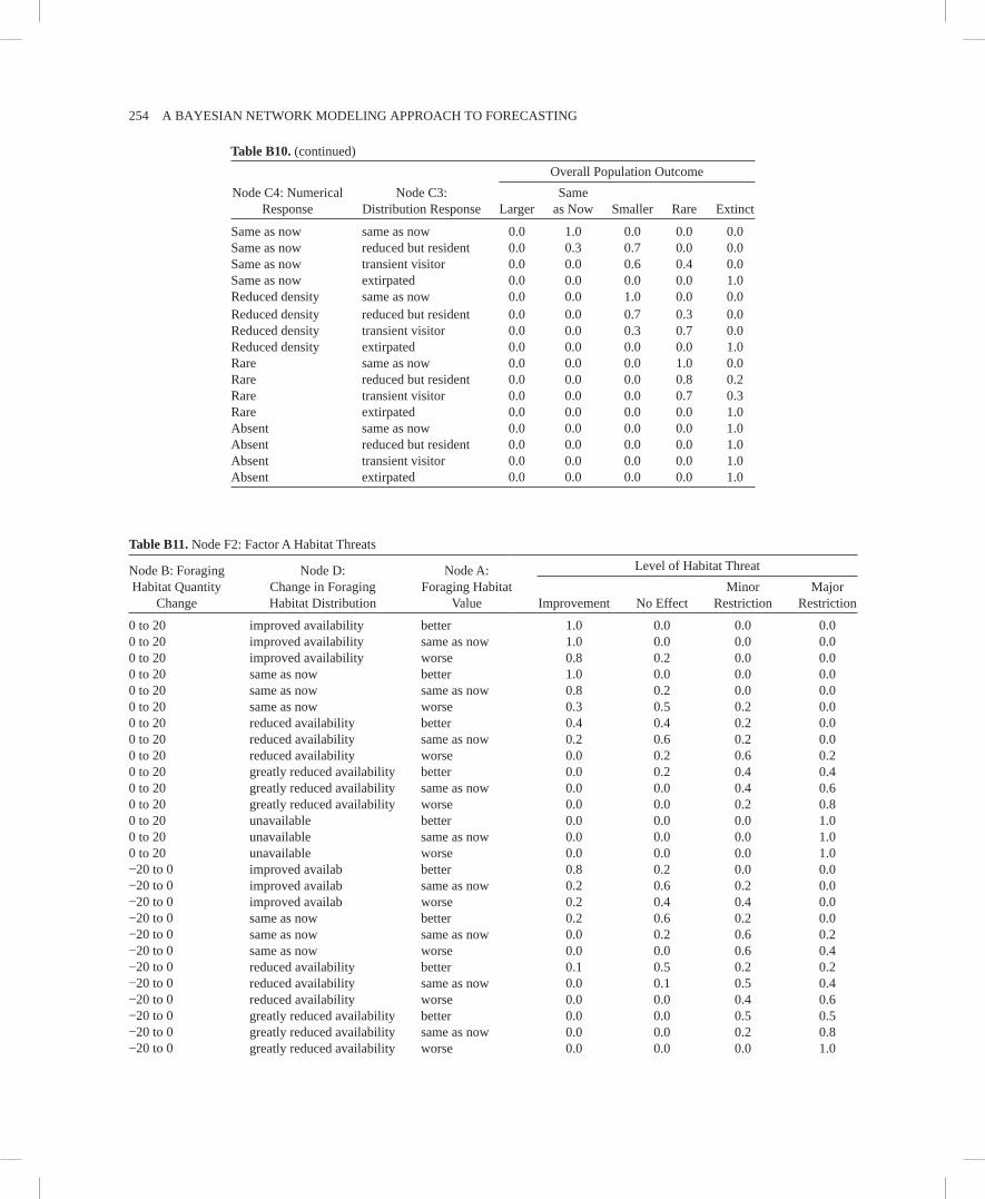
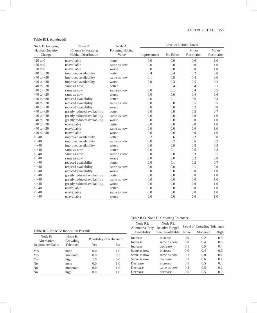
Plate 7 illustrates how distribution changes driven by changes in the sea ice appeared to be the major factor lead-ing to our dire predictions of the future for polar bears. For projection purposes, we binned the number of additional months during which the sea ice was projected to be ab-sent from the continental shelf (node C) into four categories
which included the range from 1 month less than current (−1) to ≥3 months longer than current. Similarly, we binned the maximum distance the ice edge could move away from the shelf (node N) into four categories including the range from 200 km less than current (−200) to ≥800 km additional distance. It is clear from node D (see Appendix B) that we parameterized the model such that more distant ice retreat and longer ice absence meant reduced availability of critical foraging habitats as documented by Durner et al. [2008]. Such reduced availability has been shown to have negative impacts on polar bears [Regehr et al., 2007a]. In the PBDE as an example, the general circulation models that we used to project future ice conditions, indicated values for nodes C and N will range from 1.8 to 2.2 additional months of ice absence and 234 km to 1359 km additional ice distance by mid century. Similarly, foraging habitat quantity is projected to decline between 16 and 32% by mid century. As Plate 7 illustrates even the smaller of these values for temporal and spatial retreat of sea ice place factor A node F2 (see Appen-dix B) into the category of major habitat restriction. That, in turn, pushes the distribution response toward extirpated which pushes the most probable overall population outcome into the “extinct” category. The outcome percentages in this example differ from the overall outcomes presented in Ta-ble 2 because results shown in this example occurred with-out changing any other inputs included in the full model. hence, this result provides an example of how the projected changes in sea ice alone influenced the dire projections of our BN model. Outcomes in the PBDE are even more dire when the GCMs that lose the most ice are used or when we look farther into the future. In contrast, as Table 2 and Plate 4 illustrate, outcomes are less alarming in the PBCE and AE because of the more modest changes projected for sea ice in those regions. Sensitivity analyses described below confirm this role of sea ice in driving the expected future for polar bears.
4.3. Sensitivity Analyses
Sensitivity analyses offer an opportunity to interpret model outcomes at every level. The overall population out-come was most sensitive to change in habitat quantity (node B) and temporal habitat availability (node C). The other major habitat variable, change in distance between ice and the continental shelf (node N) was the 6th most influential factor on the overall population outcome, despite its being relevant only to the polar basin ecoregions. Our BN model recognized that sea ice characteristics, and how polar bears respond to them, differed among the four ecoregions. In the SIE, for example, all members of the subpopulation are forced ashore when the ice melts entirely in summer. In the
236 A BAyESIAN NETWORk MODElING APPROACh TO FORECASTING
PBDE, by comparison, some bears retreat to shore, while most follow the sea ice as it retreats far offshore in sum-mer. The fact that ecoregion and the availability of alternate ecoregions together explained 22% of the variation in overall population outcome was further evidence of the importance of sea ice habitat and its regional differences.
Another habitat variable, “foraging habitat character” (node S1), was ranked 7th among variables having influence on the overall population outcome. This qualitative variable relating to sea ice character was included to allow for the fact that in addition to changes in quantity and distribution of sea ice, subtle changes in the composition of sea ice could affect polar bears. For example, longer open water periods and warmer winters have resulted in thinner ice in the po-lar basin region [Lindsay and Zhang, 2005; Holland et al., 2006; Belchansky et al., 2008]. Fischbach et al. [2007] con-cluded that increased prevalence of thinner and less stable ice in autumn has resulted in reduced sea ice denning among polar bears of the southern Beaufort Sea.
Observations during polar bear field work suggest that the thinning of the sea ice also has resulted in increased rough-ness and rafting among ice floes. Compared to the thicker ice that dominated the polar basin decades ago, thinner ice is more easily deformed, even late in the winter. Whether or not thinner ice is satisfactory for seals, the extensive areas of jagged pressure ridges that can result when ice is more eas-ily deformed may not be well suited to polar bear foraging. These changes appear to reduce foraging effectiveness of polar bears, and it is suspected the changes in ice conditions may have contributed to recent cannibalism and other unu-sual foraging behaviors [Stirling et al., 2008]. Also, thinner, rougher ice, interspersed with more open water, may be an impediment to the travels of young cubs. Physical difficul-ties in navigating this “new” ice environment could explain recent observed increases in mortality of first-year cubs [Rode et al., 2007]. The fact that six of the seven variables most influential on overall outcome were sea ice related and explained 87% of the variation in that outcome corroborates the well established link between polar bears and sea ice.
The 5th ranked potential stressor to which overall popu-lation outcome was sensitive was intentional takes. his-torically, the direct killing of polar bears by humans for subsistence or sport has been the biggest challenge to polar bear welfare [Amstrup, 2003]. Our model suggests that har-vest of polar bears may remain an important factor in the population dynamics of polar bears in the AE and PBCE, as sea ice retreats.
It is important to remember that there is great uncertainty in the exact way the potential stressors we modeled may change in the future. Also, the degree of uncertainty differs among the variables we included in our model. There is rela-
tively great certainty that the spatiotemporal distribution of sea ice will decline through the coming century. There is less certainty in just how much it will decline by a speci-fied decade. The short, intermediate, and long-term effects of that decline on food availability for polar bears are largely unknown [Bluhm and Gradinger, 2008]. here, we assumed that declining sea ice means declining food availability for polar bears, with the decline in food mirroring that of the sea ice. Spatiotemporal reductions in sea ice cover, how-ever, could fundamentally alter the structure and function of the Arctic ecosystem. Such changes could result in dif-ferent timing and level of productivity. It seems clear that continued declines in sea ice ultimately will mean reduced year-round food availability and declines in polar bear num-bers and distribution. We cannot rule out, however, that in-creases in productivity could result in transitory increases in food availability for bears. Such changes would not alter the ultimate predictions made here, polar bears are clearly tied to the sea ice for access to their food. Such changes could, however, alter the temporal sensitivity of our outcomes to values at input nodes.
4.4. Strength of Evidence
Our BN population stressor model projects that sea ice and sea ice related factors will be the dominant driving force affecting future distributions and numbers of polar bears through the 21st century. Despite caveats regarding the early stage of development of our BN model, there are several reasons to believe that the directions and general magnitudes of its outcomes are reasonable.
First, they are consistent with hypothesized effects of glo-bal warming on polar bears [Derocher et al., 2004] and with recent observations of how decreasing spatiotemporal distri-bution of sea ice has affected polar bears in some portions of their range [Stirling and Derocher, 1993; Stirling and Par-kinson, 2006; Stirling et al., 1999, 2007, 2008; Ainley et al., 2003; Ferguson et al., 2005; Amstrup et al., 2006; Hunter et al., 2007; Regehr et al., 2007a, 2007b; Rode et al., 2007]. The high sensitivity of our overall model outcomes to sea ice habitat changes is consistent with the recent PBSG deci-sion, based mainly on projected changes in sea ice, that polar bears should be reclassified as vulnerable [Aars et al., 2006].
Second, results of influence runs to assess the ability of on the ground activities to alter outcomes were not qualitatively different, during most time periods, from previous runs for the PBDE and SIE (Plate 6). Maintaining current conditions (other than sea ice) in the PBDE and SIE or improving con-ditions on the ground appeared to have some ability to re-duce the risk of extinction being the most probable outcome during the first couple decades of this century. This effect
AMSTRUP ET Al. 237
Plate 7. A subset of the Bayesian network model (Plate 3) illustrating why sea ice conditions projected for year 50 and beyond have such dire consequences for polar bears of the PBDE. Values of nodes N, C, and B are specified by the GCM outputs (see Tables D1a and D1b). Shown here are the input categories from the sea ice models projecting the smallest retreats of sea ice by mid century. Nodes D, F2, C3, and D1 are calculated by the Bayesian network model according to conditional probabilities specified in Appendix B. For illustration of the influence of sea ice on outcomes, we show future inputs only for the subset of nodes dealing with sea ice values here; therefore, outcomes shown here differ from those in Table 2. As illustrated in Table 2, results are more negative when other GCM outputs are used and when time frames farther into the future are examined.
238 A BAyESIAN NETWORk MODElING APPROACh TO FORECASTING
Plate 8. Area of sea ice extent (>50% ice concentration) on 16 September 2007, compared to 10 Intergovernmental Panel of Climate Change Fourth Assessment Report GCM mid century projections of ice extent for September 2045–2054 (mean ±1 standard deviation, n = 10 years). Ice extent for 16 September 2007 was calculated using near-real-time ice con-centration estimates derived with the NASA Team algorithm and distributed by the National Snow and Ice Data Center (http://nsidc.org). Note that five of the models we used in our analyses project more perennial sea ice at mid century than was observed in 2007. This suggests our projections for the future status of polar bears may be conservative.
AMSTRUP ET Al. 239
largely disappears by mid century, however, and manage-ment of localized human activities appears to have little qualitative effect on the future of polar bears in the PBDE and SIE if sea ice continues to decline as projected. The fact that sea ice has been declining more rapidly than even our minimum ice GCMs project (see below) suggests even pos-sible transitory benefits of on the ground interventions may be illusory in these ecoregions. In contrast, our BN model suggested that managing human controlled stressors could qualitatively lower the probabilities of extinction in the PBCE and AE. Such management has played an important role in the past recovery of polar bears [Amstrup, 2003] and apparently could continue to be important in regions where sea ice habitat remains.
Third, influence runs in which we specified complete un-certainty in all inputs except sea ice illustrated that in order to obtain any qualitative change in the probability of extinc-tion in any of the ecoregions, sea ice availability in future time periods must be greater than even the maximum-ice GCM projections we used (Plate 6). This eventuality may be unlikely in light of the fact that most GCMs simulate more ice than has actually been observed during 1979 to present [Durner et al., 2008; Stroeve et al., 2007]. It also seems un-likely in light of the most recent observations that September sea ice extent (15% concentration) in 2007 was 4.13 ´ 106 km2. This is lower than the previous record set in 2005 by nearly 1.2 ´ 106 km2 (National Snow and Ice Data Center, 1 October 2007 press release, available at http://nsidc.org/news/index.html). When ice extent based on a 50% concen-tration threshold, which is probably near the lower limit of ice cover useful to polar bears [Durner et al., 2008], is calcu-lated, the area in 2007 was down to approximately 3.5 ´ 106 km2. Five of the GCM models in our 10-member ensemble forecast more September sea ice in 2050 than was observed in 2007 (Plate 8). Perhaps even more telling than the overall “faster-than-forecasted” ice decline, is the observation that much of the AE, the region where we forecasted polar bears to remain until late in the century, was ice free in September 2007 (Plate 8). hence, the probability that more sea ice than projected will be available during the rest of this century seems low.
Finally, a polar bear BN population stressor model would have to be structured and parameterized very differently to project qualitatively different outcomes than we have here. yet it seems unlikely that other polar bear experts would do that. Evidence for the polar bear’s reliance on sea ice is replete. Although they are opportunistic and will take ter-restrial foods, including human refuse when available, and may benefit from such activity [Lunn and Stirling, 1985; De-rocher et al., 1993], polar bears are largely dependent on the
productivity of the marine environment. Refuse, for exam-ple, is of limited availability throughout the polar bear range, and could at best benefit relatively few individuals. Also, polar bears are inefficient in preying on terrestrial animals [Brook and Richardson, 2002; Stempniewicz, 2006]. Per-haps most importantly, polar bears have evolved a strategy designed to take advantage of the high fat content of marine mammals [Best, 1984]. Available terrestrial foods are, with few exceptions, not rich enough or cannot be gathered ef-ficiently enough to support large bodied bears [Welch et al., 1997; Rode et al., 2001; Robbins et al., 2004]. Because polar bears are the largest of the bears, it is unlikely that terrestrial arctic habitats which are depauperate from the standpoint of bear food could support them in anything like current numbers. Empirical evidence of this is provided by the fact that Arctic grizzly bears are the smallest grizzly bears found anywhere and they occur at the lowest densities [Miller et al., 1997]. habitats adjacent to present polar bear ranges just do not seem likely to support large numbers of the much larger-bodied polar bears. Although polar bears in Hudson Bay, which are forced onto land all summer, are known to consume a wide variety of foods; they gain little energetic benefit from those foods [Ramsay and Hobson, 1991]. The only foods, other than their ringed and bearded seal staples, that are known to be energetically important to polar bears in some regions are other marine mammals [Iverson et al., 2006]. Polar bears, it appears, are obligately dependent on the surface of the sea ice for capture of the prey necessary to maintain their populations.
In short, although other polar bear experts might structure a model differently and populate the conditional probability tables differently than we have here, it seems unlikely that those differences would be great enough to make a qualita-tive difference in the outcomes projected by our BN popula-tion stressor model for mid century and beyond.
5. CONClUSIONS
We used a first-generation BN population stressor model to forecast future populations of polar bears worldwide. Out-comes of this model suggested that declines in the spatiotem-poral distribution of sea ice habitat along with other potential stressors will severely impact future polar bear populations. Polar bears in the PBDE and SIE, home to approximately two thirds of the current world population will likely dis-appear by mid century. Management of localized human activities is unlikely to mitigate those mid century losses. Polar bears in and around the AE appear likely to persist late into the 21st century, especially if on-the-ground human activities, particularly human harvests, are carefully managed.
240 A BAyESIAN NETWORk MODElING APPROACh TO FORECASTING
A declining habitat base, corresponding with FWS listing factor A (habitat threats), is the overriding factor in projec-tions of declining numbers and distribution of polar bears. Other factors which correspond with FWS listing factors B, C, and E, and which could result in additional popula-tion stress on polar bears, are likely to exacerbate effects of habitat loss. To qualitatively alter outcomes projected by our models, it appears future sea ice would have to be far more extensive than is projected by even the more conservative of the general circulation models we used. Because recently observed declines in sea ice extent continue to outpace most GCM projections [Stroeve et al., 2007], more extensive sea ice in the future seems unlikely unless greenhouse gas emis-sions are reduced. This study and the others on which it was based establish that the future security of polar bears over much of their present range is threatened in an ecological context. In May 2008, Secretary of Interior Dirk kemp-thorne, upon review of this and other available information, decided this ecological threat required policy actions and declared polar bears a threatened species under the defini-tion of the Endangered Species Act [U.S. Fish and Wildlife Service, 2008].
APPENDIX A: DOCUMENTATION OF ThE BAyESIAN NETWORk POlAR BEAR
POPUlATION STRESSOR MODEl
Appendix A documents the structure of the Bayesian network (BN) population stressor model. We used the BN modeling shell Netica® (Norsys, Inc.) to create a model that represents potential influences on distribution response, nu-merical response, and overall population response of polar bears under multiple stressors, which include anthropogenic stressors, natural disturbances, and other key environmental correlates to polar bear population amount and distribution.
The BN population stressor model was created to repre-sent the knowledge and judgment of one polar bear biolo-
gist (S. Amstrup) with guidance from an ecologist modeler (B. Marcot). The general underlying influence diagram for the BN model is shown in Plate 2, and the full model is in Plate 3. A BN model consists of a series of variables rep-resented as “nodes” (boxes in Plate 3) that interact through links (arrows in Plate 3). Nodes that have no incoming ar-rows are “input nodes” (the yellow boxes in Plate 3, e.g., node T Parasites and Disease). Nodes with both incoming and outgoing arrows are summary nodes (or latent variables, e.g., node L2 Vital Rates). In our model, we also specified four of the summary nodes as listing factors used by the U.S. Fish and Wildlife Service (S. Morey, personal communica-tion, 2007). Nodes with incoming arrows but no outgoing arrows are output nodes (node D1 Overall Population Out-come). The model (Plate 3) was run by specifying condi-tions of all input nodes for each combination of ecoregion (node M), time period (node Q), and climate data source or GCM run (node R). In running the model, specifying ecore-gion automatically adjusts two of its summary nodes (D and U). The input data set (Tables D1a and D1b) also specifies time period, GCM run, and all other inputs. Nodes Q and R appear in the model unconnected as visual placeholders for displaying the basis of each model run.
Each node in this model consists of a short node name (e.g., node D1), a longer node title (e.g., Overall Population Outcome), a set of states (e.g., larger, same as now, smaller, rare, and extinct), and an underlying probability table. The probability tables consist of unconditional (or prior) prob-abilities in the input nodes, or conditional probabilities in all other nodes, the latter representing probabilities of each state as a function of (conditional upon) the states of all nodes that directly influence it.
Table A1 presents a complete list of all nodes in the model with their short code letters, titles, description, possible states, and the group (Node Set, in Netica® parlance) to which it belongs (input nodes, output node, summary node, or summary listing factor node).
Table A1. Complete list of All Nodes in the Bayesian Network Population Stressor ModelNode Name Node Title Node Description States
Input NodesT Parasites and
DiseaseAs the climate warms, regions of the Arctic are hospitable to parasites and disease agents which formerly did not survive there. Polar bears have always been free of most disease and parasite agents. Trichinella is one notable exception, but even rabies, common in the Arctic has had no significance to polar bears. Changes in other species disease vulnerability suggest that similar changes could occur in polar bears so that they could move from a position where parasites and disease are not influential on a population level to where they are influential.
influentialnot
AMSTRUP ET Al. 241
Node Name Node Title Node Description States
T2 Predation Predation on polar bears by other species is very uncommon partly because bears spend almost all of their time on the ice. With more time on land, polar bears, espe-cially young, will be subject to increased levels of predation from wolves, and perhaps grizzly bears. This will vary by region as some regions where polar bears occur have few other predators. Intraspecific predation is one behavior which is known to occur in bears. It has rarely been observed in polar bears and historically is not thought to have been influential. Recent observations of predation on other bears by large males, in regions where it has not been observed before, are consistent with the hypothesis that this sort of behavior may increase in frequency if polar bears are nutritionally stressed. At present, intraspe-cific predation is not thought to be influential at the population level anywhere in the polar bear range. It appears, however, that its frequency may be on the increase. At some point, it therefore could become influential. At very low population levels, even a minor increase in predation could be influential.
influentialnot
E Intentional Takes
This node represents direct mortalities including hunting, and collection for zoos, and management actions. It also includes research deaths even though they are not intentional. These are mortality sources that are very much controllable by regulation.
increasedsame_as_nowdecreased
T1 Contaminants Increased precipitation and glacial melt have recently resulted in greater influx of contaminants into the Arctic region from the interior of Eurasia via the large northward flowing rivers. Similarly, differing atmospheric circulation patterns have altered po-tential pathways for contaminants from lower latitudes. This node reflects the possible increase or decrease of contamination in the Arctic as a result of modified pathways. These contaminants can act to make habitat less suitable and directly affect things like survival and reproduction.The greatest likelihood seems to be that such contaminants will increase in Arctic regions (and indeed worldwide) as increasing numbers of chemicals are developed and as their persistence in the environment is belatedly determined. Some contaminants have been reduced and we have the ability to reduce others, but the record of reduction and the persistence of many of these chemicals in the environment suggests the great-est likelihood is for elevated levels in the short to medium term with some probability of stability or even declines far in the future.
elevatedsame_as_nowreduced
R4 hydrocarbons / Oil Spill
This refers to the release of oil or oil related products into polar bear habitat. Such ac-tion would result in direct mortality of bears, direct mortality of prey, and could result in displacement of bears from areas they formerly occupied. Hence, it has ramifica-tions for both habitat quality and population dynamics directly. hydrocarbon exploration and development are expanding and proposed to expand farther in the Arctic. Greater levels of such activity are most likely to increase the probability of oil spills. Also, increased shipping will result in higher levels of hydrocarbon release into Arctic waters.
J1 Tourism As sea ice extent declines spatially and temporally, access and opportunities for Arctic tourism also will increase. Increased tourism could lead to direct disturbances of polar bears as well as to increased levels of contamination. here, we address only the physical presence of more tourism and the conveyances used by tourists (vessels, land vehicles, aircraft). The greatest likelihood seems to be that tourism will increase. It could decline, however, if governments take actions to reduce interactions with increasingly stressed polar bears. however, as tourism currently accounts for essentially no limitation to polar bears this effect only comes into play when it is noted to increase. I believe that tourism will increase in all areas of the Arctic until such time as fuel
increasedsame_as_nowdecreased
Table A1. (continued)
242 A BAyESIAN NETWORk MODElING APPROACh TO FORECASTING
Node Name Node Title Node Description States
becomes too expensive for people to venture to such remote areas or in the polar basin divergent unit, when it is essentially devoid of ice, it may not attract many tourists and such activity may surge and then decline in that region. The arctic areas with more interesting coastlines etc., however, will probably see nothing but increases in tourism. Contamination that may accompany such activities, and biological effects from intro-duced organisms that may compete with residents of the food web or cause disease are covered under the nodes for contamination and parasites and disease.
B1 Bear-human interactions
This includes nonlethal takes which may increase as a result of increased human-bear interactions because of food-stressed bears more frequently entering Arctic communi-ties. Such takes can displace bears from their preferred locations and reduce habitat quality.This is separate from the similar interactions that may occur around oil and gas or other industrial sites which also can displace bears and lower habitat quality. These interactions also, however, can result in deaths as when problem bears are shot in defense of life and property. So, this node includes a component of both habitat quality and direct mortality. I believe that bear-human interactions will increase until such time as areas are devoid of bears or climate cools again and ice returns.
increasedsame_as_nowdecreased
R1 Oil and Gas Activity
This refers to the spatial effects of oil and gas activity. It refers to activities and infra-structure which may physically displace bears from habitat that was formally available to them. It also can result in direct killings of bears which become a persistent safety problem around industrial facilities. Oil companies etc. have great resources to prevent these events from leading to mortalities, but such mortalities cannot be totally avoided and are likely to increase as habitat base shrinks. I think oil and gas activity will increase in the polar basin region through mid century and then decline because resources will have been tapped. We may see some increase in exploration and development in the archipelago, however, as it becomes increas-ingly accessible.
increaseno_changedecrease
J Shipping As sea ice extent declines spatially and temporally it is predicted that shipping in Arctic regions will increase. Increased shipping could lead to direct disturbances of polar bears as well as to increased levels of contamination. here, we address only the physical presence of more vessel traffic. Contamination (bilge oil, etc.), and biological effects from introduced organisms that may compete with residents of the food web or cause disease are covered under the nodes for contamination and parasites and disease. We allow only two states here: increased and same as now, because we can think of no reason why shipping will decrease in the foreseeable future. Even if international shipping does not increase, local shipping will, because barges and vessels are more efficient ways to move fuel and freight into remote Arctic locations than aircraft.
increasedsame_as_now
F Alternate Regions Available
Are there geographic ecoregions to which bears from the subject region may effec-tively be able to relocate. This ability is contingent on other ecoregions with suitable habitats being contiguous with regions where habitat quantity or quality have degraded to the point they will not support polar bears on a seasonal or annual basis. For example, if the sea ice is deterio-rating throughout the polar basin including the Beaufort Sea and the last vestiges of ice are along the Alaskan Coast, there may be no where else to go if the ice deteriorates to an unsatisfactory state. If, however, the ice retreats to the northeast as its extent reduces, bears remaining on the ice may have access to suitable habitats in the archi-pelago or in NE Greenland. I believe that bears in the seasonal ice region and in the polar basin will be able to col-lapse into the archipelago. Ice patterns suggest that the remaining ice in the Arctic is
yesno
Table A1. (continued)
AMSTRUP ET Al. 243
Node Name Node Title Node Description States
likely to converge on the archipelago rather than form disjunct chunks of ice (although some GCMs do predict the latter, this is contrary to the historical record and the paleo-record).yes = other suitable areas are contiguousNo = other suitable regions are not contiguous
R2 Relative Ringed Seal Availability
This node expresses changes in prey availability that are likely to occur as sea ice cover declines and its character changes. This node specifically includes only the possibility that ringed seals, the mainstay of polar bears over most of their range, might change in abundance and availability. This is specific to the amount of remaining ice. That is, as sea ice declines in cover-age (which is the only way it seems possible for it to go) will the remaining habitat be more productive?Availability here refers to the combined effects of abundance and accessibility, recog-nizing that seals may occupy areas that make them less available to polar bears even if the seals are still relatively abundant. Examples of this are the recent observations of failed bear attempts to dig through solid ice (a result of the thinner ice that deforms and rafts more easily) that predominates now, and the fact that seals may simply stay in open water all summer and not be available to bears even if the seal numbers are stable. My judgment is that only in the northern part of the ice convergent zone of the polar basin and in portions of the archipelago are conditions likely to improve for ringed seal availability. And, there, such improvements are likely to be transient perhaps through mid century. increase = greater abundance or availability of ringed seals compared to nowdecrease = less abundance or availability
increasesame_as_nowdecrease
R3 Alternate Prey Availability
This node expresses changes in prey availability that are likely to occur as sea ice cover declines and its character changes. This is largely expert opinion because there is little to go on to suggest prey base change possibilities in the future. With very dif-ferent ice and other ecological differences that may accompany global warming things could occur which are totally unforeseen. Today’s experience, however, suggests that little in the way of significant alternate prey is likely to emerge to allow bears to replace traditional prey that may be greatly reduced in the future. Where alternate prey could become important is in the seasonal ice regions and the archipelago. Now, harp (Phoca groenlandicus) and hooded (Cystophora cristata) seals have become important to polar bears as they have moved farther north than histori-cally. As the ice retreats into the archipelago it is reasonable to expect that these animals may penetrate deeper into the archipelago and provide at least a transient improvement in alternate prey. It is unclear, however, that such changes could persist as bears prey on these seals which are forced onto smaller and smaller areas of ice. So, I project only transient improvements followed by decline. This node specifically addresses the possibility that alternate prey, either marine or ter-restrial, might change in a way that would allow polar bears to take advantage of it.increase = greater availability of alternate preydecrease = less opportunity for access to prey items other than ringed seals
increasesame_as_nowdecrease
S1 Foraging habitat Character
This node expresses a subjective assessment of the quality of sea ice for foraging by polar bears. Recent observations of the changes in sea ice character in the southern Beaufort Sea suggest that the later freeze-up, warmer winters, and earlier ice retreat in summer have resulted in thinner ice that more easily deforms and more frequently rafts over itself. These changes have reduced the quality of ice as a denning substrate, and may have reduced its quality as a foraging substrate since the extensive ice deforma-tion can result in ice covered refugia for ringed seals which are less likely for polar bears to get into. Also, it can result in very rough sharp pressure ridges that are hugely
more_optimalsame_as_nowless_optimal
Table A1. (continued)
244 A BAyESIAN NETWORk MODElING APPROACh TO FORECASTING
Node Name Node Title Node Description States
expansive compared to earlier years. This rough ice may also provide refuge for seals, and it also is surely difficult for polar bear COYs to negotiate as they attempt to move out onto the ice after den emergence in spring. More optimal ice is somewhat heavier and not as rough, with pressure ridges com-posed of larger ice blocks. however, it can go the other way. Very heavy stable ice in the Beaufort Sea in the past may have been limiting polar bears. This is also probably currently true in portions of the AE and in the northern part of the PBCE. So, in those areas, I expect that ice quality will at first improve with global warming and then decline. Because my only sense of this ice quality is in the polar basin, I am leaving all priors uniform for the other ice regions.
C Foraging habitat Absence Change
This node expresses the length, in months, of ice absence from the continental shelf regions currently preferred by polar bears. It corresponds to the value “proportional ice-free months” from D. Douglas’ calculations based on GCMs. This is the number of months during which the continental shelf was ice free where ice free is defined as fewer than 50% of the pixels over the shelf having less than 50% ice cover. We express this as a change from now. So the figures in this node represent the dif-ference in months between the forecasted number of ice-free months for four future time periods and the number of ice-free months for the present which is defined as the GCM model outputs for the period 2000–2009. The bears in some regions already experience protracted ice-free periods. In other re-gions they do not. The impact of the length of the ice-free period is dependent mainly upon the productivity of the environment, and has a different impact in the Beaufort Sea, for example, than it does in the currently seasonal ice environments which are, for the most part, very productive. For example, a difference in the amount of time ice was absent of GT 3 months means a mean absence of 7 or 8 months in the PBDE, and 8, 9 or 10 months in the seasonal ice zone, but only 3+ months in portions of the AE or the PBCE where ice is now present year-round.
-1 to 00 to 11 to 3>=3
B Foraging habitat Quantity Change
This node expresses the proportional change in the area of polar bear habitat over time. Polar bear habitat is expressed as the number of square km months of optimal RSF habitat in the two polar basin geographic units, and as square km months of ice over continental shelf in the other regions. Because the other regions are almost entirely shallow water areas, the habitat in those areas boils down to essentially the ice extent months over each region. We further express this as the percent change in quantity of these ice habitats, from the baseline now which is defined as the period 1996–2006. Interpreting the percent difference must take into account that a given percent change in the archipelago or the PB convergent region is a very different thing than it might be in the other two units. The absolute change in the archipelago, for example, may be very small, but because it is measured from essentially 0, it may look like a great% . These measurements are derived from the satellite record for the observational period and from the GCM outputs of sea ice for future periods.
0 to 20-20 to 0-40 to -20< -40
N Shelf Distance Change (km)
This node expresses the distance that the ice retreats from traditional autumn/winter foraging areas which are over the continental shelves and other shallow water areas within the polar basin. It is calculated by extracting the largest contiguous chunk of ice whose pixels have >50% concentration and determining the mean of the measured distances between all cells in the subpopulation unit and the nearest point within that chunk of ice. It is expressed as the difference between this mean distance calculated for the period 1996–2006 and the same mean distance calculated for the other time periods of interest. These distances are derived from the satellite record for the obser-vational period and from the GCM outputs of sea ice for future periods.
-200 to 00 to 200200 to 800>= 800
Table A1. (continued)
AMSTRUP ET Al. 245
Node Name Node Title Node Description States
Expressing this value as a change from the current time allows the model to show that conditions improve in a hind cast back to the period of 1985–1995. This measurement is available only from the polar basin ecoregions because all other management units occur in areas that are essentially all shelf. hence, the measurement of distance to shelf means nothing.
M Ecoregion Geographic region used for combining populations of polar bears. Polar_Basin_ DivergencePolar_Basin_ ConvergenceArchipelagoSeasonal_Ice
Output Nodesa
D1 Overall Population Outcome
Composite influence of numerical response and distribution response. largersame_as_nowsmallerrareextinct
C4 Numerical Response
This node represents the anticipated numerical response of polar bears based upon the sum total of the identified factors which are likely to have affected numbers of polar bears in any particular area.
This is the sum total of ecological and human factors that predict the future distribu-tion of polar bears. Reduced but Resident: habitat has changed in a way that would likely lead to a reduced spatial distribution (e.g., because of avoidance of a human development or because sea ice is still present in the area but in more limited quantity). Bears would still occur in the area, but their distribution would be more limited. Transient = habitat is seasonally limited or human activities have resulted in a situation where available ice is precluded from use on a seasonal basis.
Summary NodesC2 Pollution This is the sum of pollution effects from hydrocarbon discharges directly into arctic
waters and from other pollutants brought to the Arctic from other parts of the world. The FWS listing proposal included pollution as one of the “other factors” along with direct human bear interactions that may displace bears or otherwise make habitats less
reducedsame_as_nowelevatedgreatly_elevated
satisfactory. I viewed the main effect of pollution as a potential effect on population dynamics. Clearly, severe pollution as in an oil spill, for example, could make habitats unsatisfactory and result in direct displacement. The main effect, however, is likely to be how pollution affects immune systems, reproductive performance, and survival. hence, I have included input from this node as well as from the human disturbance node into both the habitat and the abundance side of the network by including input from factor E into both population effects and habitat effects.
C1 human Disturbance
This node expresses the combination of the changes in “other” direct human dis-turbances to polar bears. This does not include changes in sea ice habitat. Nor does it include the contamination possibilities from hydrocarbon exploration. Those are covered elsewhere. It does cover the direct bear-human interactions that can occur in association with industrial development.
reducedsame_as_nowelevatedgreatly_elevated
h Crowding Tolerance
The degree to which polar bears may tolerate increased densities that may result from migration of bears from presently occupied regions that become unsuitable to other regions already occupied by polar bears.
nonemoderatehigh
Table A1. (continued)
246 A BAyESIAN NETWORk MODElING APPROACh TO FORECASTING
Node Name Node Title Node Description States
In essence, this is the tolerance of bears to live in more crowded conditions than those at which they presently live. And, it is a function of food availability.I believe that bears have a reasonable tolerance of crowding if food is abundant or if they are in good condition while waiting for sea ice to return etc. Examples of these situations include (1) portions of the high Arctic-like near Resolute, where bear densi-ties on the sea ice in spring are apparently much higher than they are in most of the polar basin, and (2) the high densities at which polar bears occur on land in hudson Bay in summer when they are loafing and waiting for the sea ice to return. I assumed that crowding tolerance has little or no effect on outcome likelihoods until habitat quantity was reduced substantially requiring bears from one area to either per-ish or find some place else to go on at least a seasonal basis.Thereafter, if relocations of members of some subpopulations meant invading the areas occupied by other bears, crowding tolerance entered an assessment of whether or not relocation was a practical solution.
G Relocation Possible
Is it likely that polar bears displaced from one region could either seasonally or perma-nently relocate to another region in order to persist. This is a function of foraging effects (e.g., prey availability) in the alternative area (here I am specifically focusing on prey availability in the alternative area rather than the area from which the bears may have been displaced) crowding tolerance, and contiguity of habitats.
yesno
A Foraging habitat Value
This node expresses the sum total of things which may work to alter the quality of habitats available to polar bears in the future. The idea here is that sea ice is retreat-ing spatially and temporally, but is the ice that remains of comparable, better or worse quality as polar bear habitat. Our RSF values are projected into the future with the assumption that a piece of ice in 2090 that looks the same as piece of ice in 1985 has the same value to a polar bear. Perhaps because of responses we cannot foresee, it may be better seal habitat, or it may be habitat for an alternate prey. Conversely, it may be worse because of atmospheric and oceanic processes (e.g., the epontic community is less vibrant because of thinner ice which is not around for as long each year). Or it may be worse habitat because of oil and gas development, tourism, shipping etc.
bettersame_as_nowworse
D Change in Foraging habitat Distribution
This node expresses the combination of the quantitative ways the retreat of sea ice may affect use of continental shelf habitats. Our analyses indicate, in addition to reductions of total ice (and RSF Optimum ice) extent (expressed under habitat quantity), we will see seasonal retreats of the sea ice away from coastal areas now preferred by polar bears, and these retreats are projected to progressively become longer.
These changes will affect polar bears by reducing the total availability of ice substrate for bears. They also will make ice unavailable for extended periods in some regions where bears now occur year-round. This will result in the opportunity for seasonal oc-cupancy but not year-round occupancy as they have had in the past. Note that in the PBCE because it includes the North Beaufort and Queen Elizabeth and East Greenland each of which has different starting points, the values in the CPT express kind of an average. Similarly, in the Seasonal region, there is a huge difference between Hudson Bay and Foxe Basin or Baffin Bay. So, again the CPT values are a sort of an average, trying to reflect these differences.
l2 Vital Rates This expresses the combined effect of changes in survival of adult females and of young and reproductive patterns. The probabilities assigned each of the states reflects the relative importance to polar bear population dynamics of each of these vital rates to the growth of the population. This node does not reflect human influences on population growth such as hunting, or mortalities resulting from bear-human interactions. Those things, along with effects of parasites, contaminants, etc. are brought in as modifiers at the level of the next node.
improvesame_as_nowdecline
Table A1. (continued)
AMSTRUP ET Al. 247
Node Name Node Title Node Description States
U Reproduction The sum of trends in numbers of cubs produced and the effect of retreating sea ice on the ability of females to reach traditional denning areas.
increasedsame_as_nowdecreased
V1 Cub production per event
This node describes the number of cubs produced per denning attempt. fewer_than_nowsame_as_nowmore_than_now
l Juvenile Survival
Annual natural survival rate of cubs and yearlings. Note that this is conditional on sur-vival of the mother. This is the survival rate for juveniles that would occur in absence of hunting or other anthropogenic factors. Those anthropogenic factors that would influence survival are included in node F.
increaseno_changedecrease
l1 Adult Female Survival
Annual natural survival rate of sexually mature females. This is the survival rate for adult females that would occur in absence of hunting or other anthropogenic factors. Those anthropogenic factors that would influence survival are included in node F.
increaseno_changedecrease
k Adult Body Condition
Body mass index or other indicator of ability of bears to secure resources. Our analysis suggests body stature has been declining in the SBS and is inversely correlated with ice extent. Also recent analyses indicate that body condition may soon be an important predictor of survival of polar bears in ShB.
increasesame_as_nowdecrease
Summary Nodes – USFWS Listing Factors bF2 Factor A.
habitat ThreatsThis node summarizes the combined information about changes in habitat quantity and quality. It approximately reflects factor A of the proposal to list polar bears as threatened.
This node approximates the FWS listing factor B. It includes the combination of hunt-ing (harvest), take for scientific purposes, and take for zoos. It also includes mortalities from bear-human interactions etc. brought in from factor E. These all are factors which serve to modify the population changes that would be brought about without the direct local interference of humans.
fewersame_as_nowmore
A4 Factor C. Disease, predation
This node expresses probability of changing vulnerability of polar bears to diseases and parasites, and to potential increases of intraspecific predation/cannibalism.
same_as_nowworse
A6 Factor E. Other factors (natural or man-made)
This node approximately corresponds to factor E of the listing proposal. It includes factors (other than the changes in sea ice quality and quantity) which may affect habitat suitability for polar bears. Also, its effects can be directly on population dynamics fea-tures. hence, it applies directly to both the habitat and population sides of our network. Included here are effects of a variety of contaminants, including: petroleum hydrocar-bons, persistent organic pollutants, and metals. Although we do not know much quanti-tatively about effects of these contaminants at the population level, we know qualita-tively that effects on immune systems and steroid levels etc. will ultimately have such effects. We also know that oil spills will have immediate and dire effects. It also includes effects of human activities and developments which may directly affect habitat quality, including: shipping and transportation activities, habitat change, noise, spills, ballast discharge, and ecotourism. This includes disturbance but not direct killing of bears by humans as a result of DlP cases (direct killing is included under node A1). I viewed human disturbances as the most predictable in their negative effects until pol-lution levels reached their greatly elevated stage at which time, their import to future populations was judged to be great.
Descriptive (Disconnected) Nodes cQ Time Period The states for this node correspond to years −10 (historic), 0 (now), 25 (early century),
50 (mid century), 75 (late century), and 95 (end of century).historic (1985–1995)now (1996–2006)early century
Table A1. (continued)
248 A BAyESIAN NETWORk MODElING APPROACh TO FORECASTING
Node Name Node Title Node Description States
(2020–2029)mid century (2045–2055)late century (2070–2080)end of century (2090–2099)
R GCM run The states for this node correspond to the data source (either “satellite” for year −10 and 0 runs) and GCM modeling scenario (minimum, ensemble mean, or maximum) basis for a given condition.
GCM_minimumensemble_meanGCM_maximumsatellite
aOutput nodes here include the Numerical Response and Distribution Response nodes that provide summary output conditions.bU.S. Fish and Wildlife Service (USFWS) lists five listing factors. Listing factor D pertains to inadequacy of existing regulatory mecha-nisms, and was not included in the BN population stressor model because it does not correspond to any specific environmental stressor. cThese two nodes are included in the model to help denote the basis for a given model run. They are not included as environmental stress-ors per se.
Table A1. (continued)
APPENDIX B: PROBABIlITy TABlES FOR EACh NODE IN ThE BAyESIAN NETWORk MODEl
Tables B1–B19 are probability tables for each node in the BN model. (These were generated in the Netica® software.) Not included here are all input nodes (yellow coded nodes in Plate 3) because each of their prior probability tables was set to uniform distributions.
Table B1. Node A: Foraging habitat Value
Node S1: Foraging habitat Character
Node G:Relocation Possible
Value of Foraging habitat
BetterSame as
Now Worse
More optimal yes 0.7 0.3 0.0More optimal no 0.2 0.6 0.2Same as now yes 0.1 0.8 0.1Same as now no 0.0 0.8 0.2less optimal yes 0.0 0.3 0.7less optimal no 0.0 0.0 1.0
Table B2. Node A1: Factor B Overutilization
Node E:Node A6:
Factor E—Other level of OverutilizationIntentional
TakesFactors (Natural or Man-Made) Fewer
Same as Now More
Increased improvement 0.0 0.4 0.6Increased no effect 0.0 0.0 1.0Increased minor restriction 0.0 0.0 1.0Increased major restriction 0.0 0.0 1.0Same as now improvement 1.0 0.0 0.0Same as now no effect 0.0 1.0 0.0Same as now minor restriction 0.0 0.6 0.4Same as now major restriction 0.0 0.3 0.7Decreased improvement 1.0 0.0 0.0Decreased no effect 1.0 0.0 0.0Decreased minor restriction 0.0 0.8 0.2Decreased major restriction 0.0 0.6 0.4
AMSTRUP ET Al. 249
Table B3. Node A4: Factor C Disease and Predation
Node T :Parasites and Disease
Node T2:Predation
level of Disease and Predation
Same as Now Worse
Influential influential 0.0 1.0Influential not 0.3 0.7Not influential 0.7 0.3Not not 1.0 0.0
Table B4. Node A6: Factor E Other Factors Natural or Man-Made
Node C1: human Disturbance
Node C2:Pollution
level of Other Factors
Improvement No EffectMinor
RestrictionMajor
Restriction
Reduced reduced 1.0 0.0 0.0 0.0Reduced same as now 1.0 0.0 0.0 0.0Reduced elevated 0.3 0.4 0.3 0.0Reduced greatly elevated 0.0 0.3 0.3 0.4Same as now reduced 0.6 0.4 0.0 0.0Same as now same as now 0.0 1.0 0.0 0.0Same as now elevated 0.0 0.4 0.6 0.0Same as now greatly elevated 0.0 0.2 0.2 0.6Elevated reduced 0.0 0.2 0.5 0.3Elevated same as now 0.0 0.0 0.5 0.5Elevated elevated 0.0 0.0 0.4 0.6Elevated greatly elevated 0.0 0.0 0.3 0.7Greatly elevated reduced 0.0 0.0 0.3 0.7Greatly elevated same as now 0.0 0.0 0.2 0.8Greatly elevated elevated 0.0 0.0 0.1 0.9Greatly elevated greatly elevated 0.0 0.0 0.0 1.0
Table B5. Node C1: human Disturbance
Node B1:Bear-Human Interactions
Node J:Shipping
Node R1:Oil and Gas
ActivityNode J1:Tourism
level of human Disturbance
ReducedSame
as Now ElevatedGreatly Elevated
Increased increased increase increased 0.0 0.0 0.0 1.0Increased increased increase same as now 0.0 0.0 0.0 1.0Increased increased increase decreased 0.0 0.0 0.1 0.9Increased increased no change increased 0.0 0.0 0.0 1.0Increased increased no change same as now 0.0 0.0 0.1 0.9Increased increased no change decreased 0.0 0.0 0.2 0.8Increased increased decrease increased 0.0 0.0 0.3 0.7Increased increased decrease same as now 0.0 0.0 0.6 0.4Increased increased decrease decreased 0.0 0.0 0.5 0.5
250 A BAyESIAN NETWORk MODElING APPROACh TO FORECASTING
Node B1:Bear-Human Interactions
Node J:Shipping
Node R1:Oil and Gas
ActivityNode J1:Tourism
level of human Disturbance
ReducedSame
as Now ElevatedGreatly Elevated
Increased same as now increase increased 0.0 0.0 0.0 1.0Increased same as now increase same as now 0.0 0.0 0.2 0.8Increased same as now increase decreased 0.0 0.0 0.3 0.7Increased same as now no change increased 0.0 0.0 0.5 0.5Increased same as now no change same as now 0.0 0.0 0.7 0.3Increased same as now no change decreased 0.0 0.2 0.6 0.2Increased same as now decrease increased 0.0 0.0 0.7 0.3Increased same as now decrease same as now 0.0 0.2 0.7 0.1Increased same as now decrease decreased 0.0 0.4 0.6 0.0Same as now increased increase increased 0.0 0.0 0.2 0.8Same as now increased increase same as now 0.0 0.0 0.5 0.5Same as now increased increase decreased 0.0 0.2 0.6 0.2Same as now increased no change increased 0.0 0.2 0.8 0.0Same as now increased no change same as now 0.0 0.3 0.7 0.0Same as now increased no change decreased 0.0 0.5 0.5 0.0Same as now increased decrease increased 0.0 0.3 0.7 0.0Same as now increased decrease same as now 0.0 0.5 0.5 0.0Same as now increased decrease decreased 0.0 0.6 0.4 0.0Same as now same as now increase increased 0.0 0.2 0.8 0.0Same as now same as now increase same as now 0.0 0.4 0.6 0.0Same as now same as now increase decreased 0.0 0.5 0.5 0.0Same as now same as now no change increased 0.0 0.8 0.2 0.0Same as now same as now no change same as now 0.0 1.0 0.0 0.0Same as now same as now no change decreased 0.1 0.9 0.0 0.0Same as now same as now decrease increased 0.3 0.7 0.0 0.0Same as now same as now decrease same as now 0.5 0.5 0.0 0.0Same as now same as now decrease decreased 0.6 0.4 0.0 0.0Decreased increased increase increased 0.0 0.0 0.6 0.4Decreased increased increase same as now 0.0 0.2 0.6 0.2Decreased increased increase decreased 0.0 0.3 0.7 0.0Decreased increased no change increased 0.1 0.6 0.3 0.0Decreased increased no change same as now 0.2 0.6 0.2 0.0Decreased increased no change decreased 0.3 0.5 0.2 0.0Decreased increased decrease increased 0.2 0.6 0.2 0.0Decreased increased decrease same as now 0.3 0.7 0.0 0.0Decreased increased decrease decreased 0.4 0.6 0.0 0.0Decreased same as now increase increased 0.0 0.5 0.5 0.0Decreased same as now increase same as now 0.2 0.6 0.2 0.0Decreased same as now increase decreased 0.3 0.6 0.1 0.0Decreased same as now no change increased 0.5 0.5 0.0 0.0Decreased same as now no change same as now 0.7 0.3 0.0 0.0Decreased same as now no change decreased 0.8 0.2 0.0 0.0Decreased same as now decrease increased 0.9 0.1 0.0 0.0Decreased same as now decrease same as now 1.0 0.0 0.0 0.0Decreased same as now decrease decreased 1.0 0.0 0.0 0.0
Table B5. (continued)
AMSTRUP ET Al. 251
Table B6. Node C2: Pollution
Node R4:hydrocarbons/
Oil SpillNode T1:
Contaminants
level of Pollution
ReducedSame as
Now ElevatedGreatly Elevated
Increased occur elevated 0.0 0.0 0.0 1.0Increased occur same as now 0.0 0.0 0.6 0.4Increased occur reduced 0.0 0.4 0.4 0.2Same as now elevated 0.0 0.3 0.7 0.0Same as now same as now 0.0 1.0 0.0 0.0Same as now reduced 0.4 0.6 0.0 0.0Decreased occur elevated 0.3 0.5 0.2 0.0Decreased occur same as now 0.8 0.2 0.0 0.0Decreased occur reduced 1.0 0.0 0.0 0.0
Table B7. Node C3: Distribution Response
Node F2:Node A6:
Factor E—Other Node G: Distribution ResponseFactor A—
habitat ThreatsFactors (Natural or Man-Made)
Relocation Possible
Same as Now
Reduced but Resident
Transient Visitor Extirpated
Improvement improvement yes 1.0 0.0 0.0 0.0Improvement improvement no 1.0 0.0 0.0 0.0Improvement no effect yes 1.0 0.0 0.0 0.0Improvement no effect no 1.0 0.0 0.0 0.0Improvement minor restriction yes 0.9 0.1 0.0 0.0Improvement minor restriction no 0.9 0.1 0.0 0.0Improvement major restriction yes 0.8 0.1 0.1 0.0Improvement major restriction no 0.8 0.2 0.0 0.0No effect improvement yes 1.0 0.0 0.0 0.0No effect improvement no 1.0 0.0 0.0 0.0No effect no effect yes 1.0 0.0 0.0 0.0No effect no effect no 1.0 0.0 0.0 0.0No effect minor restriction yes 0.8 0.1 0.1 0.0No effect minor restriction no 0.8 0.2 0.0 0.0No effect major restriction yes 0.5 0.2 0.3 0.0No effect major restriction no 0.5 0.5 0.0 0.0Minor restriction improvement yes 0.5 0.25 0.25 0.0Minor restriction improvement no 0.5 0.5 0.0 0.0Minor restriction no effect yes 0.4 0.3 0.3 0.0Minor restriction no effect no 0.4 0.6 0.0 0.0Minor restriction minor restriction yes 0.3 0.3 0.4 0.0Minor restriction minor restriction no 0.3 0.6 0.0 0.1Minor restriction major restriction yes 0.2 0.2 0.6 0.0Minor restriction major restriction no 0.2 0.5 0.0 0.3Major restriction improvement yes 0.0 0.3 0.35 0.35Major restriction improvement no 0.0 0.3 0.0 0.7Major restriction no effect yes 0.0 0.2 0.4 0.4Major restriction no effect no 0.0 0.2 0.0 0.8Major restriction minor restriction yes 0.0 0.1 0.45 0.45Major restriction minor restriction no 0.0 0.1 0.0 0.9Major restriction major restriction yes 0.0 0.0 0.3 0.7Major restriction major restriction no 0.0 0.0 0.0 1.0
252 A BAyESIAN NETWORk MODElING APPROACh TO FORECASTING
Table B8. Node C4: Numerical Response
Node l2:Vital Rates
Node A1:Factor B—
Overutilization
Node A4:Factor C—
Disease and Predation
Numerical ResponseIncreased Density
Same as Now
Reduced Density Rare Absent
Improve fewer same as now 1.0 0.0 0.0 0.0 0.0Improve fewer worse 0.5 0.25 0.25 0.0 0.0Improve same as now same as now 0.8 0.2 0.0 0.0 0.0Improve same as now worse 0.5 0.25 0.25 0.0 0.0Improve more same as now 0.3 0.35 0.35 0.0 0.0Improve more worse 0.1 0.4 0.5 0.0 0.0Same as now fewer same as now 0.2 0.8 0.0 0.0 0.0Same as now fewer worse 0.0 0.8 0.2 0.0 0.0Same as now same as now same as now 0.0 1.0 0.0 0.0 0.0Same as now same as now worse 0.0 0.3 0.7 0.0 0.0Same as now more same as now 0.0 0.2 0.8 0.0 0.0Same as now more worse 0.0 0.0 1.0 0.0 0.0Decline fewer same as now 0.0 0.5 0.5 0.0 0.0Decline fewer worse 0.0 0.3 0.7 0.0 0.0Decline same as now same as now 0.0 0.0 1.0 0.0 0.0Decline same as now worse 0.0 0.0 0.75 0.25 0.0Decline more same as now 0.0 0.0 0.4 0.4 0.2Decline more worse 0.0 0.0 0.2 0.4 0.4
Table B9. Node D: Change in Foraging habitat Distribution
Node M: Ecoregion
Node C:Foraging habitat Absence Change
Node N:Shelf Distance
Change
Distribution of Foraging habitatImproved
AvailabilitySame as
NowReduced
AvailabilityGreatly Reduced
Availability Unavailable
Polar basin divergent -1 to 0 -200 to 0 1.0 0.0 0.0 0.0 0.0Polar basin divergent -1 to 0 0 to 200 0.8 0.2 0.0 0.0 0.0Polar basin divergent -1 to 0 200 to 800 0.2 0.6 0.2 0.0 0.0Polar basin divergent -1 to 0 >= 800 0.0 0.4 0.6 0.0 0.0Polar basin divergent 0 to 1 -200 to 0 0.5 0.5 0.0 0.0 0.0Polar basin divergent 0 to 1 0 to 200 0.0 0.2 0.8 0.0 0.0Polar basin divergent 0 to 1 200 to 800 0.0 0.0 0.5 0.5 0.0Polar basin divergent 0 to 1 >= 800 0.0 0.0 0.25 0.5 0.25Polar basin divergent 1 to 3 -200 to 0 0.2 0.4 0.4 0.0 0.0Polar basin divergent 1 to 3 0 to 200 0.0 0.0 0.5 0.3 0.2Polar basin divergent 1 to 3 200 to 800 0.0 0.0 0.2 0.4 0.4Polar basin divergent 1 to 3 >= 800 0.0 0.0 0.0 0.2 0.8Polar basin divergent >= 3 -200 to 0 0.0 0.3 0.5 0.2 0.0Polar basin divergent >= 3 0 to 200 0.0 0.0 0.2 0.4 0.4Polar basin divergent >= 3 200 to 800 0.0 0.0 0.0 0.1 0.9Polar basin divergent >= 3 >= 800 0.0 0.0 0.0 0.0 1.0Polar basin convergent -1 to 0 -200 to 0 1.0 0.0 0.0 0.0 0.0Polar basin convergent -1 to 0 0 to 200 0.8 0.2 0.0 0.0 0.0Polar basin convergent -1 to 0 200 to 800 0.6 0.4 0.0 0.0 0.0Polar basin convergent -1 to 0 >= 800 0.4 0.6 0.0 0.0 0.0Polar basin convergent 0 to 1 -200 to 0 1.0 0.0 0.0 0.0 0.0Polar basin convergent 0 to 1 0 to 200 0.6 0.4 0.0 0.0 0.0Polar basin convergent 0 to 1 200 to 800 0.2 0.4 0.4 0.0 0.0Polar basin convergent 0 to 1 >= 800 0.0 0.2 0.8 0.0 0.0Polar basin convergent 1 to 3 -200 to 0 0.6 0.4 0.0 0.0 0.0
AMSTRUP ET Al. 253
Node M: Ecoregion
Node C:Foraging habitat Absence Change
Node N:Shelf Distance
Change
Distribution of Foraging habitatImproved
AvailabilitySame as
NowReduced
AvailabilityGreatly Reduced
Availability Unavailable
Polar basin convergent 1 to 3 0 to 200 0.1 0.5 0.4 0.0 0.0Polar basin convergent 1 to 3 200 to 800 0.0 0.3 0.7 0.0 0.0Polar basin convergent 1 to 3 >= 800 0.0 0.0 1.0 0.0 0.0Polar basin convergent >= 3 -200 to 0 0.4 0.6 0.0 0.0 0.0Polar basin convergent >= 3 0 to 200 0.1 0.3 0.5 0.1 0.0Polar basin convergent >= 3 200 to 800 0.0 0.2 0.6 0.2 0.0Polar basin convergent >= 3 >= 800 0.0 0.0 0.7 0.3 0.0Archipelago -1 to 0 -200 to 0 0.0 1.0 0.0 0.0 0.0Archipelago -1 to 0 0 to 200 0.0 1.0 0.0 0.0 0.0Archipelago -1 to 0 200 to 800 0.0 1.0 0.0 0.0 0.0Archipelago -1 to 0 >= 800 0.0 1.0 0.0 0.0 0.0Archipelago 0 to 1 -200 to 0 0.6 0.4 0.0 0.0 0.0Archipelago 0 to 1 0 to 200 0.6 0.4 0.0 0.0 0.0Archipelago 0 to 1 200 to 800 0.6 0.4 0.0 0.0 0.0Archipelago 0 to 1 >= 800 0.6 0.4 0.0 0.0 0.0Archipelago 1 to 3 -200 to 0 0.4 0.6 0.0 0.0 0.0Archipelago 1 to 3 0 to 200 0.4 0.6 0.0 0.0 0.0Archipelago 1 to 3 200 to 800 0.4 0.6 0.0 0.0 0.0Archipelago 1 to 3 >= 800 0.4 0.6 0.0 0.0 0.0Archipelago >= 3 -200 to 0 0.0 0.6 0.4 0.0 0.0Archipelago >= 3 0 to 200 0.0 0.6 0.4 0.0 0.0Archipelago >= 3 200 to 800 0.0 0.6 0.4 0.0 0.0Archipelago >= 3 >= 800 0.0 0.6 0.4 0.0 0.0Seasonal ice -1 to 0 -200 to 0 0.5 0.5 0.0 0.0 0.0Seasonal ice -1 to 0 0 to 200 0.5 0.5 0.0 0.0 0.0Seasonal ice -1 to 0 200 to 800 0.5 0.5 0.0 0.0 0.0Seasonal ice -1 to 0 >= 800 0.5 0.5 0.0 0.0 0.0Seasonal ice 0 to 1 -200 to 0 0.0 0.2 0.6 0.2 0.0Seasonal ice 0 to 1 0 to 200 0.0 0.2 0.6 0.2 0.0Seasonal ice 0 to 1 200 to 800 0.0 0.2 0.6 0.2 0.0Seasonal ice 0 to 1 >= 800 0.0 0.2 0.6 0.2 0.0Seasonal ice 1 to 3 -200 to 0 0.0 0.0 0.2 0.4 0.4Seasonal ice 1 to 3 0 to 200 0.0 0.0 0.2 0.4 0.4Seasonal ice 1 to 3 200 to 800 0.0 0.0 0.2 0.4 0.4Seasonal ice 1 to 3 >= 800 0.0 0.0 0.2 0.4 0.4Seasonal ice >= 3 -200 to 0 0.0 0.0 0.0 0.1 0.9Seasonal ice >= 3 0 to 200 0.0 0.0 0.0 0.1 0.9Seasonal ice >= 3 200 to 800 0.0 0.0 0.0 0.1 0.9Seasonal ice >= 3 >= 800 0.0 0.0 0.0 0.1 0.9
Table B9. (continued)
Table B10. Node D1: Overall Population Outcome
Node C4: Numerical Response
Node C3:Distribution Response
Overall Population Outcome
largerSame
as Now Smaller Rare Extinct
Increased density same as now 1.0 0.0 0.0 0.0 0.0Increased density reduced but resident 0.3 0.5 0.2 0.0 0.0Increased density transient visitor 0.1 0.3 0.3 0.3 0.0Increased density extirpated 0.0 0.0 0.0 0.0 1.0
254 A BAyESIAN NETWORk MODElING APPROACh TO FORECASTING
Table B11. Node F2: Factor A habitat Threats
Node B: Foraging habitat Quantity
Change
Node D:Change in Foraging habitat Distribution
Node A:Foraging habitat
Value
level of habitat Threat
Improvement No EffectMinor
RestrictionMajor
Restriction
0 to 20 improved availability better 1.0 0.0 0.0 0.00 to 20 improved availability same as now 1.0 0.0 0.0 0.00 to 20 improved availability worse 0.8 0.2 0.0 0.00 to 20 same as now better 1.0 0.0 0.0 0.00 to 20 same as now same as now 0.8 0.2 0.0 0.00 to 20 same as now worse 0.3 0.5 0.2 0.00 to 20 reduced availability better 0.4 0.4 0.2 0.00 to 20 reduced availability same as now 0.2 0.6 0.2 0.00 to 20 reduced availability worse 0.0 0.2 0.6 0.20 to 20 greatly reduced availability better 0.0 0.2 0.4 0.40 to 20 greatly reduced availability same as now 0.0 0.0 0.4 0.60 to 20 greatly reduced availability worse 0.0 0.0 0.2 0.80 to 20 unavailable better 0.0 0.0 0.0 1.00 to 20 unavailable same as now 0.0 0.0 0.0 1.00 to 20 unavailable worse 0.0 0.0 0.0 1.0-20 to 0 improved availab better 0.8 0.2 0.0 0.0-20 to 0 improved availab same as now 0.2 0.6 0.2 0.0-20 to 0 improved availab worse 0.2 0.4 0.4 0.0-20 to 0 same as now better 0.2 0.6 0.2 0.0-20 to 0 same as now same as now 0.0 0.2 0.6 0.2-20 to 0 same as now worse 0.0 0.0 0.6 0.4-20 to 0 reduced availability better 0.1 0.5 0.2 0.2-20 to 0 reduced availability same as now 0.0 0.1 0.5 0.4-20 to 0 reduced availability worse 0.0 0.0 0.4 0.6-20 to 0 greatly reduced availability better 0.0 0.0 0.5 0.5-20 to 0 greatly reduced availability same as now 0.0 0.0 0.2 0.8-20 to 0 greatly reduced availability worse 0.0 0.0 0.0 1.0
Node C4: Numerical Response
Node C3:Distribution Response
Overall Population Outcome
largerSame
as Now Smaller Rare Extinct
Same as now same as now 0.0 1.0 0.0 0.0 0.0Same as now reduced but resident 0.0 0.3 0.7 0.0 0.0Same as now transient visitor 0.0 0.0 0.6 0.4 0.0Same as now extirpated 0.0 0.0 0.0 0.0 1.0Reduced density same as now 0.0 0.0 1.0 0.0 0.0Reduced density reduced but resident 0.0 0.0 0.7 0.3 0.0Reduced density transient visitor 0.0 0.0 0.3 0.7 0.0Reduced density extirpated 0.0 0.0 0.0 0.0 1.0Rare same as now 0.0 0.0 0.0 1.0 0.0Rare reduced but resident 0.0 0.0 0.0 0.8 0.2Rare transient visitor 0.0 0.0 0.0 0.7 0.3Rare extirpated 0.0 0.0 0.0 0.0 1.0Absent same as now 0.0 0.0 0.0 0.0 1.0Absent reduced but resident 0.0 0.0 0.0 0.0 1.0Absent transient visitor 0.0 0.0 0.0 0.0 1.0Absent extirpated 0.0 0.0 0.0 0.0 1.0
Table B10. (continued)
AMSTRUP ET Al. 255
Node B: Foraging habitat Quantity
Change
Node D:Change in Foraging habitat Distribution
Node A:Foraging habitat
Value
level of habitat Threat
Improvement No EffectMinor
RestrictionMajor
Restriction
-20 to 0 unavailable better 0.0 0.0 0.0 1.0-20 to 0 unavailable same as now 0.0 0.0 0.0 1.0-20 to 0 unavailable worse 0.0 0.0 0.0 1.0-40 to -20 improved availability better 0.4 0.4 0.2 0.0-40 to -20 improved availability same as now 0.1 0.5 0.4 0.0-40 to -20 improved availability worse 0.0 0.3 0.5 0.2-40 to -20 same as now better 0.1 0.4 0.4 0.1-40 to -20 same as now same as now 0.0 0.1 0.4 0.5-40 to -20 same as now worse 0.0 0.0 0.4 0.6-40 to -20 reduced availability better 0.0 0.1 0.6 0.3-40 to -20 reduced availability same as now 0.0 0.0 0.5 0.5-40 to -20 reduced availability worse 0.0 0.0 0.2 0.8-40 to -20 greatly reduced availability better 0.0 0.0 0.3 0.7-40 to -20 greatly reduced availability same as now 0.0 0.0 0.0 1.0-40 to -20 greatly reduced availability worse 0.0 0.0 0.0 1.0-40 to -20 unavailable better 0.0 0.0 0.0 1.0-40 to -20 unavailable same as now 0.0 0.0 0.0 1.0-40 to -20 unavailable worse 0.0 0.0 0.0 1.0< -40 improved availability better 0.2 0.6 0.2 0.0< -40 improved availability same as now 0.0 0.2 0.6 0.2< -40 improved availability worse 0.0 0.0 0.5 0.5< -40 same as now better 0.0 0.1 0.6 0.3< -40 same as now same as now 0.0 0.0 0.3 0.7< -40 same as now worse 0.0 0.0 0.2 0.8< -40 reduced availability better 0.0 0.1 0.2 0.7< -40 reduced availability same as now 0.0 0.0 0.1 0.9< -40 reduced availability worse 0.0 0.0 0.0 1.0< -40 greatly reduced availability better 0.0 0.0 0.0 1.0< -40 greatly reduced availability same as now 0.0 0.0 0.0 1.0< -40 greatly reduced availability worse 0.0 0.0 0.0 1.0< -40 unavailable better 0.0 0.0 0.0 1.0< -40 unavailable same as now 0.0 0.0 0.0 1.0< -40 unavailable worse 0.0 0.0 0.0 1.0
Table B11. (continued)
Table B12. Node G: Relocation PossibleNode F:
Alternative Node h:
Crowding Possibility of RelocationRegions Available Tolerance yes No
yes none 0.0 1.0yes moderate 0.8 0.2yes high 1.0 0.0No none 0.0 1.0No moderate 0.0 1.0No high 0.0 1.0
Table B13. Node h: Crowding ToleranceNode R2:
Alternative PreyNode R3:
Relative Ringed level of Crowding ToleranceAvailability Seal Availability None Moderate high
Increase increase 0.0 0.2 0.8Increase same as now 0.0 0.4 0.6Increase decrease 0.1 0.5 0.4 Same as now increase 0.0 0.4 0.6Same as now same as now 0.1 0.8 0.1Same as now decrease 0.3 0.6 0.1Decrease increase 0.1 0.5 0.4Decrease same as now 0.3 0.5 0.2Decrease decrease 0.5 0.5 0.0
256 A BAyESIAN NETWORk MODElING APPROACh TO FORECASTING
Table B14. Node k: Adult Body Condition
Node F2: Factor A—habitat Threats
Quality of Adult Body ConditionIncrease Same as Now Decrease
Increase increase increased 1.0 0.0 0.0Increase increase same as now 1.0 0.0 0.0Increase increase decreased 0.6 0.4 0.0Increase no change increased 0.9 0.1 0.0Increase no change same as now 0.8 0.2 0.0Increase no change decreased 0.7 0.2 0.1Increase decrease increased 0.3 0.5 0.2Increase decrease same as now 0.2 0.5 0.3Increase decrease decreased 0.0 0.4 0.6No change increase increased 0.7 0.3 0.0No change increase same as now 0.6 0.4 0.0No change increase decreased 0.2 0.5 0.3No change no change increased 0.2 0.8 0.0No change no change same as now 0.0 1.0 0.0No change no change decreased 0.0 0.8 0.2No change decrease increased 0.0 0.6 0.4No change decrease same as now 0.0 0.5 0.5No change decrease decreased 0.0 0.3 0.7Decrease increase increased 0.2 0.4 0.4Decrease increase same as now 0.0 0.6 0.4Decrease increase decreased 0.0 0.5 0.5Decrease no change increased 0.1 0.5 0.4Decrease no change same as now 0.0 0.4 0.6Decrease no change decreased 0.0 0.3 0.7Decrease decrease increased 0.0 0.2 0.8Decrease decrease same as now 0.0 0.0 1.0Decrease decrease decreased 0.0 0.0 1.0
Table B15. Node l: Juvenile SurvivalNode k:
Adult BodyNode l1:
Adult Female Juvenile SurvivalCondition Survival Increase No Change Decrease
Increase increase 1.0 0.0 0.0Increase no change 0.7 0.3 0.0Increase decrease 0.0 0.4 0.6Same as now increase 0.8 0.2 0.0Same as now no change 0.0 1.0 0.0Same as now decrease 0.0 0.2 0.8Decrease increase 0.0 0.6 0.4Decrease no change 0.0 0.3 0.7Decrease decrease 0.0 0.0 1.0
Increase improvement 1.0 0.0 0.0Increase no effect 0.8 0.2 0.0Increase minor restriction 0.1 0.6 0.3Increase major restriction 0.0 0.5 0.5Same as now improvement 0.5 0.5 0.0Same as now no effect 0.0 1.0 0.0Same as now minor restriction 0.0 0.6 0.4Same as now major restriction 0.0 0.3 0.7Decrease improvement 0.0 0.4 0.6Decrease no effect 0.0 0.2 0.8Decrease minor restriction 0.0 0.1 0.9Decrease major restriction 0.0 0.0 1.0
AMSTRUP ET Al. 257
Table B18. Node U: Reproduction
Node V1:Node N:
Shelf Distance Rate of ReproductionNode M: Ecoregion Cub Production per Event Change (km) Increased Same as Now Decreased
Polar basin divergent fewer than now -200 to 0 0.0 0.3 0.7Polar basin divergent fewer than now 0 to 200 0.0 0.2 0.8Polar basin divergent fewer than now 200 to 800 0.0 0.0 1.0Polar basin divergent fewer than now >= 800 0.0 0.0 1.0Polar basin divergent same as now -200 to 0 0.7 0.3 0.0Polar basin divergent same as now 0 to 200 0.0 1.0 0.0Polar basin divergent same as now 200 to 800 0.0 0.3 0.7Polar basin divergent same as now >= 800 0.0 0.0 1.0Polar basin divergent more than now -200 to 0 1.0 0.0 0.0Polar basin divergent more than now 0 to 200 0.5 0.5 0.0Polar basin divergent more than now 200 to 800 0.0 0.5 0.5Polar basin divergent more than now >= 800 0.0 0.0 1.0Polar basin convergent fewer than now -200 to 0 0.0 0.5 0.5Polar basin convergent fewer than now 0 to 200 0.0 0.4 0.6Polar basin convergent fewer than now 200 to 800 0.0 0.3 0.7Polar basin convergent fewer than now >= 800 0.0 0.2 0.8Polar basin convergent same as now -200 to 0 1.0 0.0 0.0Polar basin convergent same as now 0 to 200 0.5 0.5 0.0Polar basin convergent same as now 200 to 800 0.2 0.6 0.2Polar basin convergent same as now >= 800 0.0 0.5 0.5Polar basin convergent more than now -200 to 0 1.0 0.0 0.0Polar basin convergent more than now 0 to 200 0.8 0.2 0.0Polar basin convergent more than now 200 to 800 0.4 0.4 0.2Polar basin convergent more than now >= 800 0.2 0.4 0.4Archipelago fewer than now -200 to 0 0.0 0.2 0.8Archipelago fewer than now 0 to 200 0.0 0.2 0.8Archipelago fewer than now 200 to 800 0.0 0.2 0.8Archipelago fewer than now >= 800 0.0 0.2 0.8Archipelago same as now -200 to 0 0.2 0.6 0.2Archipelago same as now 0 to 200 0.2 0.6 0.2Archipelago same as now 200 to 800 0.2 0.6 0.2Archipelago same as now >= 800 0.2 0.6 0.2Archipelago more than now -200 to 0 0.8 0.2 0.0Archipelago more than now 0 to 200 0.8 0.2 0.0Archipelago more than now 200 to 800 0.8 0.2 0.0Archipelago more than now >= 800 0.8 0.2 0.0Seasonal ice fewer than now -200 to 0 0.0 0.2 0.8Seasonal ice fewer than now 0 to 200 0.0 0.2 0.8Seasonal ice fewer than now 200 to 800 0.0 0.2 0.8Seasonal ice fewer than now >= 800 0.0 0.2 0.8Seasonal ice same as now -200 to 0 0.2 0.6 0.2Seasonal ice same as now 0 to 200 0.2 0.6 0.2Seasonal ice same as now 200 to 800 0.2 0.6 0.2Seasonal ice same as now >= 800 0.2 0.6 0.2Seasonal ice more than now -200 to 0 0.8 0.2 0.0Seasonal ice more than now 0 to 200 0.8 0.2 0.0Seasonal ice more than now 200 to 800 0.8 0.2 0.0Seasonal ice more than now >= 800 0.8 0.2 0.0
258 A BAyESIAN NETWORk MODElING APPROACh TO FORECASTING
Table C1. Sensitivity Group 1: Sensitivity of Overall Population OutcomeNode Mutual Information Node Title
Test 1: Sensitivity of Node D1—Overall Population Outcome to All Input NodesB 0.12974 Foraging habitat Quantity ChangeC 0.04876 foraging habitat absence changeM 0.04166 ecoregionF 0.02590 alternate regions availableE 0.01607 intentional takesN 0.01393 shelf distance change (km)S1 0.01037 foraging habitat characterB1 0.00821 bear-human interactionsT 0.00506 parasites and diseaseR4 0.00271 hydrocarbons/oil spillR1 0.00254 oil and gas activityJ 0.00198 shippingT2 0.00092 predationT1 0.00073 contaminantsR3 0.00069 alternate prey availabilityR2 0.00065 relative ringed seal availabilityJ1 0.00040 tourism
Test 2. Sensitivity of Node D1—Overall Population Outcome to Listing Factor NodesF2 0.66422 factor a: habitat threatsA1 0.05253 factor b: direct mortalitiesA6 0.03150 factor e: other factors (natural or man-made)A4 0.01039 factor c: disease, predation
Test 3: Sensitivity of Node D1—Overall Population Outcome to Intermediate Nodesa
l2 0.56624 vital ratesl 0.54067 juvenile survivall1 0.54057 adult female survivalk 0.53353 adult body conditionV1 0.44705 cub production per event
APPENDIX C: RESUlTS OF SENSITIVITy ANAlySES OF ThE BAyESIAN NETWORk
POPUlATION STRESSOR MODEl
Tables C1 and C2 present the results of conducting a se-ries of sensitivity analyses of the Bayesian network popu-lation stressor model discussed in the text (also see Plate 3). Sensitivity analysis reveals the degree to which se-
lected input or summary variables influence the calculated values of a specified output variable. Tables C1 and C2 present results of 10 sensitivity tests on various summary and output nodes in the model (see text for explanation of calculations). Note that mutual information is also called entropy reduction. All tests were conducted using the Baye-sian network modeling software package Netica® (Norsys, Inc.).
AMSTRUP ET Al. 259
Table C2. Sensitivity Group 2: Sensitivity of SubmodelsNode Mutual Information Node Title
Test 5: Sensitivity of Node A4—Factor C Disease and PredationT 0.39016 parasites and diseaseT2 0.06593 predation
Test 6: Sensitivity of Node C2—PollutionR4 0.69005 hydrocarbons/oil spillT1 0.13542 contaminants
Test 7: Sensitivity of Node C1—Human DisturbanceB1 0.45796 bear-human interactionsR1 0.12450 oil and gas activityJ 0.08941 shippingJ1 0.01729 tourism
Test 8: Sensitivity of Node A—Foraging Habitat ValueS1 0.51589 foraging habitat characterF 0.04028 alternate regions availableR3 0.00105 alternate prey availabilityR2 0.00100 relative ringed seal
availabilityTest 9: Sensitivity of Node D—Change in Foraging Habitat DistributionM 0.33239 ecoregionC 0.32674 foraging habitat absence
changeN 0.06131 shelf distance change (km)
Node Mutual Information Node Title
U 0.24141 reproductionD 0.19993 change in foraging habitat distributionG 0.04235 relocation possibleA 0.02866 foraging habitat valueC1 0.01856 human disturbanceh 0.00537 crowding toleranceC2 0.00432 pollution
Test 4: Sensitivity of Node D1—Overall Population Outcome to Selected Intermediate Nodesb
F2 0.66422 factor a: habitat threatsl2 0.56624 vital ratesA1 0.05253 factor b: direct mortalitiesG 0.04235 relocation possibleA6 0.03150 factor e: other factors (natural or man-made)A4 0.01039 factor c: disease and predationaThis does not include the listing factor nodes included in test 2 above.bThis includes all (6) nodes that are two links distant from the output node.
Table C1. (continued)
260 A BAyESIAN NETWORk MODElING APPROACh TO FORECASTING
Node Mutual Information Node Title
Test 10: Sensitivity of Node L2—Vital Ratesl1 1.04302 adult female survivall 1.04048 juvenile survivalF2 0.93484 factor a: habitat threatsk 0.92047 adult body conditionV1 0.64819 cub production per eventU 0.34420 reproductionM 0.04217 ecoregionN 0.01843 shelf distance change (km)
Table C2. (continued)
APPENDIX D: INPUT VAlUES USED IN ThE BAyESIAN NETWORk POlAR BEAR POPUlATION
STRESSOR MODEl FOR EACh OF FOUR POlAR BEAR ECOREGIONS
Tables D1a and D1b present input data values used in the Bayesian network polar bear population stressor model for
each of four polar bear ecoregions. Separate input values were provided for each time period projected and for the en-semble mean of general circulation model outputs as well as for individual GCMs that projected the maximum and mini-mum sea ice remaining in each time period.
Table D1a. Input Data Values for Nodes B, C, N, S1, R3, R2, and F Used in the Bayesian Network Polar Bear Population Stressor Model for Each of Four Polar Bear Ecoregions
Time PeriodaSea Ice Data
Source
Node and Variable Nameb
B: Foraging habitat
Quantity Change
(%)
C: Foraging habitat Absence Change
N: Shelf
Distance Changec
(km)
S1: Foraging habitat
Character
R3: Alternative
Prey Availability
R2: Relative
Ringed Seal Availability
F: Alternative
Regions Available
Seasonal Ice Ecoregionyear -10 Satellite data 17.14 -0.7 NA more_optimal decrease increase yesyear 0 Satellite data 0.00 0.0 NA same_as_now same_as_now same_as_now yesyear 25 GCM minimum -4.17 0.1 NA same_as_now same_as_now decrease yesyear 50 GCM minimum -10.36 1.0 NA same_as_now decrease decrease yesyear 75 GCM minimum -31.89 2.5 NA less_optimal decrease decrease yesyear 95 GCM minimum -32.11 2.7 NA less_optimal decrease decrease yesyear 25 Ensemble mean -4.65 0.3 NA same_as_now same_as_now decrease yesyear 50 Ensemble mean -14.62 1.0 NA same_as_now decrease decrease yesyear 75 Ensemble mean -25.75 1.6 NA less_optimal decrease decrease yesyear 95 Ensemble mean -27.83 1.8 NA less_optimal decrease decrease yesyear 25 GCM maximum -0.05 0.1 NA same_as_now same_as_now decrease yesyear 50 GCM maximum -6.71 0.7 NA same_as_now decrease decrease yesyear 75 GCM maximum -21.16 1.3 NA same_as_now decrease decrease yesyear 95 GCM maximum -21.69 1.7 NA same_as_now decrease decrease yes
Archipelago Ecoregionyear -10 Satellite data 3.21 -0.5 NA less_optimal same_as_now decrease noyear 0 Satellite data 0.00 0.0 NA same_as_now same_as_now same_as_now noyear 25 GCM minimum -6.16 0.6 NA more_optimal same_as_now increase noyear 50 GCM minimum -13.79 1.1 NA more_optimal increase increase noyear 75 GCM minimum -20.71 2.0 NA same_as_now decrease decrease no
AMSTRUP ET Al. 261
Time PeriodaSea Ice Data
Source
Node and Variable Nameb
B: Foraging habitat
Quantity Change
(%)
C: Foraging habitat Absence Change
N: Shelf
Distance Changec
(km)
S1: Foraging habitat
Character
R3: Alternative
Prey Availability
R2: Relative
Ringed Seal Availability
F: Alternative
Regions Available
year 95 GCM minimum -24.30 2.3 NA same_as_now decrease decrease noyear 25 Ensemble mean -2.35 0.2 NA more_optimal same_as_now increase noyear 50 Ensemble mean -11.93 1.5 NA more_optimal increase increase noyear 75 Ensemble mean -20.06 2.4 NA same_as_now increase decrease noyear 95 Ensemble mean -22.16 2.5 NA same_as_now decrease decrease noyear 25 GCM maximum -0.08 0.0 NA more_optimal same_as_now increase noyear 50 GCM maximum -3.43 0.0 NA more_optimal increase increase noyear 75 GCM maximum -18.02 2.7 NA more_optimal increase increase noyear 95 GCM maximum -20.85 2.3 NA same_as_now decrease decrease no
aTime period is expressed as the central year in each decade for which projections were made.
bUnits of measure at each node are B, percentile change from present in the annual sum of habitat quantity; C, difference between present and future number of ice-free months; N, difference between present and future distance between the edge of the continental shelf and the edge of the pack ice; and discrete states for all other nodes. See Figure 3 for allowable states at each node.cNA stands for not applicable; shelf distance change only applies to the polar basin ecoregions.
Table D1a. (continued)
262 A BAyESIAN NETWORk MODElING APPROACh TO FORECASTING
Table D1b. Input Data Values for Nodes J1, B1, R1, J, R4, T1, E, T, and T2 Used in the Bayesian Network Polar Bear Population Stressor Model for Each of Four Polar Bear Ecoregionsa
Polar Basin Convergent Ecoregionyear -10 same_as_now reduced same_as_now not notyear 0 same_as_now same_as_now same_as_now not notyear 25 same_as_now same_as_now same_as_now not notyear 50 increased_occurrence elevated decreased influential influentialyear 75 increased_occurrence elevated decreased influential influentialyear 95 increased_occurrence elevated decreased influential influentialyear 25 same_as_now same_as_now same_as_now not notyear 50 increased_occurrence elevated decreased influential influentialyear 75 increased_occurrence elevated decreased influential influentialyear 95 increased_occurrence elevated decreased influential influentialyear 25 same_as_now same_as_now same_as_now not notyear 50 increased_occurrence elevated decreased influential influentialyear 75 increased_occurrence elevated decreased influential influentialyear 95 increased_occurrence elevated decreased influential influentialaTime period is expressed as the central year in each decade for which projections were made. bUnits of measure are discrete states at each node. See Figure 3 for allowable states at each node.
Table D1b. (continued)
AMSTRUP ET Al. 265
Acknowledgments. Principal funding for this project was pro-vided by the U.S. Geological Survey. We thank G. S. york and k. S. Simac for logistical support on this project and for keeping the office going while we were preoccupied. We thank G. M. Durner, E. V. Regehr, M. Runge, and S. Morey for valuable discussions and k. Oakley for effective and insightful project management. We are grateful to W. L. Thompson, T. Starfield, N. Lunn, and B. Taylor for helpful reviews of earlier versions of our model and this paper. We acknowledge the modeling groups for making their sea ice simulations and projections available for analysis, the Program for Climate Model Diagnosis and Intercomparison (PCMDI) for collecting and archiving the CMIP3 model output, and the WCRP’s Working Group on Coupled Modeling (WGCM) for organizing the model data analysis activity. The WCRP CMIP3 multimodel data set is supported by the Office of Science, U.S. Department of Energy. Any use of trade, product, or company names in this publi-cation is for descriptive purposes only and does not imply endorse-ment by the U.S. Government.
REFERENCES
Aalders, I. (2008), Modeling land-use decision behavior with Baye-sian belief networks. Ecol. Soc., 13(1), article 16.
Aars, J., N. J. lunn, and A. E. Derocher (2006), Polar bears: Pro-ceedings of the fourteenth working meeting of the IUCN/SSC Polar Bear Specialist Group, Occas. Pap. IUCN Species Surv. Comm. 32, 189 pp., Int. Union for Conserv. Nature and Nat. Re-sour., Gland, Switzerland.
Ainley, D. G., C. T. Tynan, and I. Stirling (2003), Sea ice: A criti-cal habitat for polar marine mammals and birds, in Sea Ice: An Introduction to Its Physics, Chemistry, Biology and Geology, edited by D. N. Thomas and G. S. Dieckmann, pp. 240–266, Blackwell Sci., Malden, Mass.
Amstrup, S. C. (1986), Polar bear, in Audubon Wildlife Report, edited by R. l. DiSilvestro, pp. 790–804, Natl. Audubon Soc., New york.
Amstrup, S. C. (2000), Polar bear, in The Natural History of an Oil Field: Development and Biota, edited by J. C. Truett and S. R. Johnson, pp. 133–157, Academic, New york.
Amstrup, S. C. (2003), Polar bear, in Wild Mammals of North America. Biology, Management, and Conservation, 2nd ed., edited by G. A. Feldhammer, B. C. Thompson, and J. A. Chap-man, pp. 587–610, Johns hopkins Univ. Press, Baltimore, Md.
Amstrup, S. C., and D. P. DeMaster (1988), Polar bear—Ursus maritimus, in Selected Marine Mammals of Alaska: Species Ac-counts With Research and Management Recommendations, ed-ited by J. W. lentfer, pp. 39–56, Mar. Mammal Comm., Wash-ington, D. C.
Amstrup, S. C., and C. Gardner (1994), Polar bear maternity den-ning in the Beaufort Sea, J. Wildl. Manage., 58(1), 1–10.
Amstrup, S. C., G. M. Durner, I. Stirling, N. J. lunn, and F. Messier (2000), Movements and distribution of polar bears in the Beau-fort Sea, Can. J. Zool., 78, 948–966.
Amstrup, S. C., T. l. McDonald, and G. M. Durner (2004), Us-ing satellite radiotelemetry data to delineate and manage wildlife populations, Wildl. Soc. Bull., 32(3), 661–679.
Amstrup, S. C., G. M. Durner, I. Stirling, and T. l. McDonald (2005), Allocating harvests among polar bear stocks in the Beau-fort Sea, Arctic, 58(3), 247–259.
Amstrup, S. C., I. Stirling, T. S. Smith, C. Perham, and G. W. Thie-mann (2006), Recent observations of intraspecific predation and cannibalism among polar bears in the southern Beaufort Sea, Po-lar Biol., 29(11), 997–1002, doi:10.1007/s00300-006-0142-5.
Amstrup, S. C., B. G. Marcot, and D. C. Douglas (2007), Forecast-ing the range-wide status of polar bears at selected times in the 21st century, administrative report, 123 pp., U.S. Geol. Surv., Alaska Sci. Cent., Anchorage, Alaska. (Available at http://www.usgs.gov/newsroom/special/polar_bears/)
Arthur, S. M., B. F. J. Manly, l. l. McDonald, and G. W. Garner (1996), Assessing habitat selection when availability changes, Ecology, 77(1), 215–227.
Barrett, G. W. (1981), Stress ecology: An integrative approach, in Stress Effects on Natural Ecosystems, edited by G. W. Barrett and R. Rosenberg, pp. 3–12, John Wiley, New york.
Belchansky, G. I., D. C. Douglas, and N. G. Platonov (2005), Spa-tial and temporal variations in the age structure of Arctic sea ice, Geophys. Res. Lett., 32, l18504, doi:10.1029/2005Gl023976.
Belchansky, G. I., D. C. Douglas, and N. G. Platonov (2008), Fluc-tuating Arctic sea ice thickness changes estimated by an in situ learned and empirically forced neural network model, J. Clim., 21(4), 716–729, doi:10.1175/2007JClI1787.1
Best, R. C. (1984), Digestibility of ringed seals by the polar bear, Can. J. Zool., 63, 1033–1036.
Bluhm, B. A., and R. Gradinger (2008), Regional variability in food availability for Arctic marine mammals, Ecol. Appl., 18, suppl., S77–S96.
Bollen, k. A. (1989), Structural Equations With Latent Variables, 528 pp., John Wiley, New york.
Brook, R. k., and E. S. Richardson (2002), Observations of polar bear predatory behaviour toward caribou, Arctic, 55(2), 193–196.
Cain, J. (2001), Planning improvements in natural resources man-agement: Guidelines for using Bayesian networks to support the planning and management of development programmes in the water sector and beyond, report, 124 pp., Crowmarsh Gifford, Cent. for Ecol. and hydrol., Wallingford, U. k.
Calvert, W., and I. Stirling (1990), Interactions between polar bears and overwintering walruses in the central Canadian high Arctic, Int. Conf. Bear Res. Manage., 8, 351–356.
Cavalieri, D., C. Parkinson, P. Gloersen, and h. J. Zwally (1996), Sea ice concentrations from Nimbus-7 SMMR and DMSP SSM/I passive microwave data, http://nsidc.org/data/nsidc-0051.html, Natl. Snow and Ice Data Cent., Boulder, Colo. (updated 2006)
Comiso, J. C. (2002), A rapidly declining perennial sea ice cover in the Arctic, Geophys. Res. Lett., 29(20), 1956, doi:10.1029/2002Gl015650.
Comiso, J. C. (2006), Abrupt decline in the Arctic winter sea ice cover, Geophys. Res. Lett., 33, l18504, doi:10.1029/2006Gl027341.
266 A BAyESIAN NETWORk MODElING APPROACh TO FORECASTING
Das, B. (2000), Representing uncertainty using Bayesian networks, report, 58 pp., Def. Sci. and Technol. Organ., Dep. of Def., Salis-bury, S. Aust., Australia.
Derocher, A. E., D. Andriashek, and I. Stirling (1993), Terrestrial foraging by polar bears during the ice-free period in western hudson Bay, Arctic, 46(3), 251–254.
Derocher, A. E., Ø. Wiig, and G. Bangjord (2000), Predation of Svalbard reindeer by polar bears, Polar Biol., 23(10), 675–678.
Derocher, A. E., Ø. Wiig, and M. Andersen (2002), Diet compo-sition of polar bears in Svalbard and the western Barents Sea, Polar Biol., 25(6), 448–452.
Derocher, A. E., N. J. lunn, and I. Stirling (2004), Polar bears in a warming climate, Integr. Comp. Biol., 44, 163–176.
DeWeaver, E. (2007), Uncertainty in climate model projections of Arctic sea ice decline, administrative report, 47 pp., U.S. Geol. Surv., Anchorage, Alaska.
Durner, G. M., and S. C. Amstrup (1995), Movements of a polar bear from northern Alaska to northern Greenland, Arctic, 48(4), 338–341.
Durner, G. M., D. C. Douglas, R. M. Nielson, and S. C. Amstrup (2006), Model for autumn pelagic distribution of adult female polar bears in the Chukchi Sea, 1987–1994, final report to U.S. Fish and Wildlife Service, 67 pp., U.S. Geol. Surv., Alaska Sci. Cent., Anchorage, Alaska.
Durner, G. M., et al. (2008), Predicting 21st century polar bear habitat distribution from global climate models, Ecol. Monogr., in press.
Dyck, M. G., and S. Romber (2007), Observations of a wild polar bear (Ursus maritimus) successfully fishing Artic charr (Sal-velinus alpinus) and Fourhorn sculpin (Myoxocephalus quad-ricornis), Polar Biol., 30(12), 1625–1628, doi:10.1007/s00300-007-0338-3.
Ferguson, S. H., M. K. Taylor, E. W. Born, A. Rosing-Asvid, and F. Messier (1999), Determinants of home range size for polar bears (Ursus maritimus), Ecol. Lett., 2, 311–318.
Ferguson, S. H., M. K. Taylor, and F. Messier (2000), Influence of sea ice dynamics on habitat selection by polar bears, Ecology, 81(3), 761–772.
Ferguson, S. h., I. Stirling, and P. Mcloughlin (2005), Climate change and ringed seal (Phoca hispida) recruitment in western hudson Bay, Mar. Mammal Sci., 21(1), 121–135.
Fischbach, A. S., S. C. Amstrup, and D. C. Douglas (2007), land-ward and eastward shift of Alaskan polar bears denning associ-ated with recent sea ice changes, Polar Biol., 30(11), 1395–1405, doi:1007/s00300-007-0300-4.
Furnell, D. J., and D. Oolooyuk (1980), Polar bear predation on ringed seals in ice-free water, Can. Field Nat., 94, 88–89.
Garner, G. W., S. T. knick, and D. C. Douglas (1990), Seasonal movements of adult female polar bears in the Bering and Chuk-chi Seas, Int. Conf. Bear Res. Manage, 8, 219–226.
Garner, G. W., S. C. Amstrup, I. Stirling, and S. E. Belikov (1994), Habitat considerations for polar bears in the North Pacific Rim, Trans. North Am. Wildl. Nat. Resour. Conf., 59, 111–120.
Ginzburg, l. R., l. B. Slobodkin, k. Johnson, and A. G. Bindman (1982), Quasiextinction probabilities as a measure of impact on population growth, Risk Anal., 2, 171–181.
Guisan, A., A. lehmann, S. Ferrier, M. Austin, J. M. C. Overton, R. Aspinall, and T. hastie (2006), Making better biogeographi-cal predictions of species’ distributions, J. Appl. Ecol., 43(3), 386–392.
hammill, M. O., and T. G. Smith (1991), The role of predation in the ecology of the ringed seal in Barrow Strait, Northwest Ter-ritories, Canada, Mar. Mammal Sci., 7(2), 123–135.
holland, M. M., C. M. Bitz, and B. Tremblay (2006), Future abrupt reductions in the summer Arctic sea ice, Geophys. Res. Lett., 33, l23503, doi:10.1029/2006Gl028024.
hufthammer, A. k. (2001), The Weichselian (c. 115,000–10,000 B.P.) vertebrate fauna of Norway, Boll. Soc. Paleontol. Ital., 40(2), 201–208.
hunter, C. M., h. Caswell, M. C. Runge, E. V. Regehr, S. C. Am-strup, and I. Stirling (2007), Polar bears in the southern Beaufort Sea II: Demography and population growth in relation to sea ice conditions, administrative report, 46 pp., U.S. Geol. Surv., An-chorage, Alaska. (Available at http://www.usgs.gov/newsroom/special/polar_bears/)
Ingolfsson, O., and O. Wiig (2007), Fossil find on Svalbard high-lights the natural history of the polar bear (Ursus maritimus), Eos Trans. AGU, 88(52), Fall Meet. Suppl., Abstract GC11B-01.
Iverson, S. J., I. Stirling, and S. l. C. land (2006), Spatial, tem-poral, and individual variation in the diets of polar bears across the Canadian Arctic: Indicators of changes in prey populations and environment, in Top Predators in Marine Ecosystems, edited by I. Boyd, S. W. Wanless, and C. J. Camphuysen, pp. 98–117, Cambridge Univ. Press, Cambridge, U. k.
Jensen, F. V. (2001), Bayesian Networks and Decision Graphs, 284 pp., Springer, New york.
Johnson, C. J., and M. P. Gillingham (2004), Mapping uncertainty: Sensitivity of wildlife habitat ratings to expert opinion, J. Appl. Ecol., 41(6), 1032–1041.
kingsley, M. C. S. (1998), The numbers of ringed seals (Phoca hispida) in Baffin Bay and associated waters, in Ringed Seals in the North Atlantic, edited by M. P. Heide-Jorgensen and C. lydersen, pp. 181–196, NAAMCO Sci. Publ., vol. 1, N. Atl. Mar. Mammal Comm., Tromsø, Norway.
lindsay, R. W., and J. Zhang (2005), The thinning of Arctic sea ice, 1988–2003: have we passed a tipping point?, J. Clim., 18(22), 4879–4894.
Lunn, N. J., and I. Stirling (1985), The significance of supplemental food to polar bears during the ice-free period of Hudson Bay, Can. J. Zool., 63, 2291–2297.
lunn, N. J., I. Stirling, and D. Andriashek (1995), Movements and distribution of polar bears in the northeastern Beaufort Sea and western M’Clure Strait, final report to the Inuvialuit Wildlife Management Advisory Committee, Can. Wildlife Serv., Edmon-ton, Alberta, Canada.
lunn, N. J., S. Schliebe, and E. W. Born (Eds.) (2002), Polar bears, in Proceedings of the Thirteenth Working Meeting of the IUCN/SSC Polar Bear Specialist Group, Occas. Pap. IUCN Species Survival Comm. 26, 153 pp., Int. Union for Conserv. of Nature and Nat. Resour., Gland, Switzerland.
Manly, B. F. J., l. l. McDonald, D. l. Thomas, T. l. McDonald, and W. P. Erickson (2002), Resource Selection by Animals: Sta-
AMSTRUP ET Al. 267
tistical Design and Analysis for Field Studies, kluwer Acad., Norwell, Mass.
Marcot, B. G. (1990), Testing your knowledge base, in Expert Sys-tems: A Software Methodology for Modern Applications, edited by P. G. Raeth, pp. 438–443, IEEE Comput. Soc. Press, los Alamitos, Calif.
Marcot, B. G. (2006), Characterizing species at risk I: Modeling rare species under the Northwest Forest Plan, Ecol. Soc., 11(2), article 10.
Marcot, B. G., M. G. Raphael, and k. h. Berry (1983), Monitor-ing wildlife habitat and validation of wildlife-habitat relation-ships models, Trans. North Am. Wildl. Nat. Resour. Conf., 48, 315–329.
Marcot, B. G., R. S. holthausen, M. G. Raphael, M. M. Rowland, and M. J. Wisdom (2001), Using Bayesian belief networks to evaluate fish and wildlife population viability under land man-agement alternatives from an environmental impact statement, For. Ecol. Manage., 153(1–3), 29–42.
Marcot, B. G., J. D. Steventon, G. D. Sutherland, and R. k. Mc-Cann (2006), Guidelines for developing and updating Bayesian belief networks applied to ecological modeling and conserva-tion, Can. J. For. Res., 36, 3063–3074.
Maslanik, J. A., S. Drobot, C. Fowler, W. Emery, and R. Barry (2007), On the Arctic climate paradox and the continuing role of atmospheric circulation in affecting sea ice conditions, Geophys. Res. Lett., 34, l03711, doi:10.1029/2006Gl028269.
McCann, R., B. G. Marcot, and R. Ellis (2006), Bayesian belief networks: Applications in natural resource management, Can. J. For. Res., 36, 3053–3062.
McConkey, k. R., and D. R. Drake (2006), Flying foxes cease to function as seed dispersers long before they become rare, Ecol-ogy, 87(2), 271–276.
Meehl, G. A., C. Covey, T. Delworth, M. latif, B. McAvaney, J. F. B. Mitchell, R. J. Stouffer, and k. E. Taylor (2007a), The WCRP CMIP3 multimodel dataset: A new era in climate change research, Bull. Am. Meteorol. Soc., 88(9), 1383–1394.
Meehl, G. A., et al. (2007b), Global climate projections, in Cli-mate Change 2007: The Physical Science Basis: Contribution of Working Group I to the Fourth Assessment Report of the Intergovernmental Panel on Climate Change, edited by S. Solo-mon et al., pp. 747–845, Cambridge Univ. Press, Cambridge, U. k.
Meier, W. N., J. Stroeve, and F. Fetterer (2007), Whither Arctic sea ice? A clear signal of decline regionally, seasonally and extend-ing beyond the satellite record, Ann. Glaciol., 46, 428–434.
Messier, F., M. k. Taylor, and M. A. Ramsay (1992), Seasonal activity patterns of female polar bears (Ursus maritimus) in the Canadian Arctic as revealed by satellite telemetry, J. Zool., 226, 219–229.
Miller, S. D., et al. (1997), Brown and black bear density estima-tion in Alaska using radiotelemetry and replicated mark-resight techniques, Wildl. Monogr., 133, 1–55.
Nakićenović, N., et al. (2000), Special Report on Emissions Sce-narios: A Special Report of Working Group III of the Inter-govermental Panel on Climate Change, 599 pp., Cambridge Univ. Press, Cambridge, U. k.
Neopolitan, R. E. (2003), Learning Bayesian Networks, 674 pp., Prentice hall, New york.
Obbard, M. E., M. R. l. Cattet, T. Moody, l. R. Walton, D. Potter, J. Inglis, and C. Chenier (2006), Temporal trends in the body con-dition of southern hudson Bay polar bears, Res. Inf. Note 3, 8 pp., Ontario Minist. of Nat. Resour., Peterborough, Ont., Canada.
Ogi, M., and J. M. Wallace (2007), Summer minimum Arctic sea ice extent and associated summer atmospheric circulation, Geo-phys. Res. Lett., 34, l12705, doi:10.1029/2007Gl029897.
Otway, N. M., C. J. A. Bradshaw, and R. G. harcourt (2004), Es-timating the rate of quasiextinction of the Australian grey nurse shark (Carcharias taurus) population using deterministic age- and stage-classified models, Biol. Conserv., 119, 341–350.
Ovsyanikov, N. (1996), Polar Bears: Living With the White Bear, 144 pp., Voyager, Stillwater, Minn.
Parovshchikov, V. y. (1964), A study on the population of polar bear, Ursus (Thalarctos) maritimus Phipps, of Franz Joseph land, Acta Soc. Zool. Bohemoslov., 28, 167–177.
Pomeroy, l. R. (1997), Primary production in the Arctic Ocean estimated from dissolved oxygen, J. Mar. Syst., 10, 1–8.
Pourret, O., P. Naïm, and B. G. Marcot (Eds.) (2008), Bayesian Be-lief Networks: A Practical Guide to Applications, 432 pp., John Wiley, Chichester, U. k.
Ramsay, M. A., and k. A. hobson (1991), Polar bears make little use of terrestrial food webs: Evidence from stable-carbon iso-tope analysis, Oecologia, 86, 598–600.
Ramsay, M. A., and I. Stirling (1984), Interactions of wolves and polar bears in northern Manitoba, J. Mammal., 65, 693–694.
Raphael, M. G., M. J. Wisdom, M. M. Rowland, R. S. holthausen, B. C. Wales, B. G. Marcot, and T. D. Rich (2001), Status and trends of habitats of terrestrial vertebrates in relation to land management in the interior Columbia River Basin, For. Ecol. Manage., 153(1–3), 63–87.
Rayner, N. A., D. E. Parker, E. B. horton, C. k. Folland, l. V. Al-exander, D. P. Rowell, E. C. kent, and A. kaplan (2003), Global analyses of sea surface temperature, sea ice, and night marine air temperature since the late nineteenth century, J. Geophys. Res., 108(D14), 4407, doi:10.1029/2002JD002670.
Regehr, E. V., C. M. hunter, h. Caswell, S. C. Amstrup, and I. Stirling (2007a), Polar bears in the Southern Beaufort Sea I: Survival and breeding in relation to sea ice conditions, 2001-2006, administrative report, 45 pp., U.S. Geol. Surv., Anchor-age, Alaska. (Available at http://www.usgs.gov/newsroom/spe-cial/polar_bears/)
Regehr, E. V., N. J. lunn, S. C. Amstrup, and I. Stirling (2007b), Effects of earlier sea ice breakup on survival and population size of polar bears in western hudson Bay, J. Wildlife Manage., 71(8), 2673–2683.
Rigor, I. G., and J. M. Wallace (2004), Variations in the age of Arctic sea-ice and summer sea-ice extent, Geophys. Res. Lett., 31, l09401, doi:10.1029/2004Gl019492.
Rigor, I. G., J. M. Wallace, and R. l. Colony (2002), Response of sea ice to the Arctic Oscillation, J. Clim., 15(18), 2648–2663.
Robbins, C. T., C. C. Schwartz, and l. A. Felicetti (2004), Nutri-tional ecology of ursids: A review of newer methods and man-agement implications, Ursus, 15(2), 161–171.
268 A BAyESIAN NETWORk MODElING APPROACh TO FORECASTING
Rode, k. D., C. T. Robbins, and l. A. Shipley (2001), Constraints on herbivory by grizzly bears, Oecologia, 128, 62–71.
Rode, k. D., S. C. Amstrup, and E. V. Regehr (2007), Polar bears in the southern Beaufort Sea III: Stature, mass, and cub recruit-ment in relationship to time and sea ice extent between 1982 and 2007, administrative report, 28 pp., U.S. Geol. Surv., An-chorage, Alaska. (Available at http://www.usgs.gov/newsroom/ special/polar_bears/)
Russell, R. h. (1975), The food habits of polar bears of James Bay and southwest hudson Bay in summer and autumn, Arctic, 28(2), 117–129.
Sakshaug, E. (2004), Primary and secondary production in the Arc-tic seas, in Organic Carbon Cycle in the Arctic Ocean, edited by R. Stein and R. W. Macdonald, pp. 57–81, Springer, New york.
Schweinsburg, R. E., and l. J. lee (1982), Movement of four satel-lite-monitored polar bears in Lancaster Sound, Northwest Ter-ritories, Arctic, 35(4), 504–511.
Sekercioglu, C. h., G. C. Daily, and P. R. Ehrlich (2004), Ecosys-tem consequences of bird declines, Proc. Natl. Acad. Sci. U. S. A., 101(52), 18,042–18,047.
Serreze, M. C., M. M. holland, and J. Stroeve (2007), Perspectives on the Arctic’s shrinking sea-ice cover, Science, 315(5818), 1533–1536.
Smith, A. E., and M. R. J. hill (1996), Polar bear, Ursus maritimus, depredation of Canada goose, Branta canadensis, nests, Can. Field Nat., 110, 339–340.
Smith, T. G. (1980), Polar bear predation of ringed and bearded seals in the land-fast sea ice habitat, Can. J. Zool., 58, 2201–2209.
Smith, T. G. (1985), Polar bears, Ursus maritimus, as predators of belugas, Delphinapterus leucas, Can. Field Nat., 99, 71–75.
Smith, T. G., and B. Sjare (1990) Predation of belugas and narwals by polar bears in nearshore areas of the Canadian high Arctic, Arctic, 43(2), 99–102.
Smith, T. G., and I. Stirling (1975), The breeding habitat of the ringed seal (Phoca hispida), The birth lair and associated struc-tures, Can. J. Zool., 53, 1297–1305.
Stefansson, V. (1921), The Friendly Arctic, 361 pp., Macmillan, New york.
Stempniewicz, l. (1993), The polar bear Ursus maritimus feed-ing in a seabird colony in Frans Josef land, Polar Res., 12(1), 33–36.
Stempniewicz, l. (2006), Polar bear predatory behaviour toward molting barnacle geese and nesting Glaucous Gulls on Spitsber-gen, Arctic, 59(3), 247–251.
Stirling, I. (1974), Midsummer observations on the behavior of wild polar bears (Ursus maritimus), Can. J. Zool., 52, 1191–1198.
Stirling, I. (1980), The biological importance of polynyas in the Canadian Arctic, Arctic, 33(2), 303–315.
Stirling, I. (1990), Polar bears and oil: Ecologic perspectives, in Sea Mammals and Oil: Confronting the Risks, edited by J. R. Geraci and D. J. St. Aubin, pp. 223–234, Academic, San Diego, Calif.
Stirling, I., and A. E. Derocher (1993), Possible impacts of climatic warming on polar bears, Arctic, 46(3), 240–245.
Stirling, I., and N. J. Lunn (1997), Environmental fluctuations in Arctic marine ecosystems as reflected by variability in reproduc-tion of polar bears and ringed seals, in Ecology of Arctic En-
vironments, Br. Ecol. Soc. Spec. Publ., vol. 13, edited by S. J. Woodin and M. Marquiss, pp. 167–181, Blackwell Sci., Oxford, U. k.
Stirling, I., and N. A. Øritsland (1995), Relationships between esti-mates of ringed seal (Phoca hispida) and polar bear ( Ursus mar-itimus) populations in the Canadian Arctic, Can. J. Fish. Aquat. Sci., 52, 2594–2612.
Stirling, I., and C. l. Parkinson (2006), Possible effects of climate warming on selected populations of polar bears (Ursus mariti-mus) in the Canadian Arctic, Arctic, 59(3), 261–275.
Stirling, I., h. Cleator, and T. G. Smith (1981), Marine mammals, in Polynyas in the Canadian Arctic, edited by I. Stirling and h. Cleator, pp. 45–48, Occas. Pap. 45, Can. Wildlife Serv., Ottawa, Ont., Canada.
Stirling, I., N. J. Lunn, and J. Iacozza (1999), Long-term trends in the population ecology of polar bears in western hudson Bay in relation to climatic change, Arctic, 52(3), 294–306.
Stirling, I., T. l. McDonald, E. S. Richardson, and E. V. Regehr (2007), Polar bear population status in the Northern Beaufort Sea, administrative report, 33 pp., U.S. Geol. Surv., Anchorage, Alaska. (Available at http://www.usgs.gov/newsroom/special/polar_bears/)
Stirling, I., E. Richardson, G. W. Thiemann, and A. E. Derocher (2008), Unusual predation attempts of polar bears on ringed seals in the southern Beaufort Sea: Possible significance of changing spring ice conditions, Arctic, 61(1), 14–22.
Stroeve, J., M. M. holland, W. Meier, T. Scambos, and M. Serreze (2007), Arctic sea ice decline: Faster than forecast, Geophys. Res. Lett., 34, l09501, doi:10.1029/2007Gl029703.
Talbot, S. l., and G. F. Shields (1996), Phylogeography of brown bears (Ursus arctos) of Alaska and paraphyly within the Ursidae, Mol. Phylogenet. Evol., 5, 477–494.
Townsend, C. W. (Ed.) (1911), Captain Cartwright and His Labra-dor Journal, 385 pp., Dana Estes, Boston, Mass.
U.S. Fish and Wildlife Service (2007), Endangered and threatened wildlife and plants; 12-month petition finding and proposed rule to list the polar bear (Ursus maritimus) as threatened throughout its range, Fed. Regist., 72(5), 1064–1099.
U.S. Fish and Wildlife Service (2008), Endangered and threatened wildlife and plants; determination of threatened status for the polar bear (Ursus maritimus) throughout its range, Fed. Regist., 73(95), 28,212–28,303.
Uusitalo, l. (2007), Advantages and challenges of Bayesian net-works in environmental modeling, Ecol. Modell., 203, 312–318.
Watts, P. D., and S. E. hansen (1987), Cyclic starvation as a re-productive strategy in the polar bear, Symp. Zool. Soc. London, 57, 305–318.
Welch, C. A., J. keay, k. C. kendall, and C. T. Robbins (1997), Constraints on frugivory by bears, Ecology, 78(4), 1105–1119.
S. C. Amstrup, Alaska Science Center, U.S. Geological Survey, Anchorage, Ak 99508, USA. ([email protected])
D. C. Douglas, Alaska Science Center, U.S. Geological Survey, Juneau, Ak 99801, USA.
B. G. Marcot, Pacific Northwest Research Station, USDA Forest Service, Portland, OR 97204, USA.