A BEHAVIORAL APPROACH TO A STRATEGIC MARKET GAME 1

A BEHAVIORAL APPROACH TO A STRATEGIC MARKET GAME

MARTIN SHUBIK AND NICOLAAS J. VRIEND

1. Introduction 1

In this paper we interlink a dynamic programming, a game theory and a behav-ioral simulation approach to the same problem of economic exchange. We arguethat the success of mathematical economics and game theory in the study of thestationary state of a population of microeconomic decision makers has helped tocreate an unreasonable faith that many economists have placed in models of ”ra-tional behavior”.

The size and complexity of the strategy sets for even a simple infinite horizonexchange economy are so overwhelmingly large that it is reasonably clear thatindividuals do not indulge in exhaustive search over even a large subset of thepotential strategies. Furthermore unless one restricts the unadorned definition ofa noncooperative equilibrium to a special form such as a perfect noncooperativeequilibrium, almost any outcome can be enforced as an equilibrium by a suffi-ciently ingenious selection of strategies. In essence, almost anything goes, unlessthe concept of what constitutes a satisfactory solution to the game places limits onpermitted or expected behavior.

Much of microeconomics has concentrated on equilibrium conditions. Gen-eral equilibrium theory provides a central example. When one considers infinitehorizon models one is faced with the unavoidable task of taking into account howto treat expectations concerning the future state of the system. An aestheticallypleasing, but behaviorally unsatisfactory and empirically doubtful way of han-dling this problem is to introduce the concept of ”rational expectations”. Math-ematically this boils down to little more than extending the definition of a non-cooperative equilibrium in such a way that the system ”bites its tail” and time

1We wish to thank Paola Manzini and participants at the Society of Computational Economicsconference in Austin, TX, for helpful comments. Stays at the Santa Fe Institute, its hospitality andits stimulating environment are also gratefully acknowledged.

262 MARTIN SHUBIK AND NICOLAAS J. VRIEND

disappears from the model. Stated differently one imposes the requirement thatexpectations and initial conditions are related in such a manner that the systemis stationary. All expectations are self-confirming and consistent. From any twopoints in time, if the system is in the same physical state overall behavior will beidentical.

Unfortunately, even if we were to assume that the property of consistency ofexpectations were a critical aspect of human life, the noncooperative equilibriumanalysis would not tell us how to get there. Even if one knows that an equilibriumexists, suppose that the system is started away from equilibrium, the rational ex-pectations requirement is not sufficient to tell us if it will converge to equilibrium.Furthermore as the equilibrium is generally not unique the dynamics is probablyhighly influenced by the location of the initial conditions.

The approach adopted here is to select a simple market model where we canprove that for at least a class of expectations formation rules, a unique stationarystate exists and we can calculate the actual state. Then we consider what are therequirements to study the dynamics of the system if the initial conditions are suchthat the system starts at a position away from the equilibrium state.

The model studied provides an example where the existence of a perfect non-cooperative equilibrium solution can be established for a general class of gameswith a continuum of agents.

In the game studied a full process model must be specified. Thus a way ofinterpreting the actions of the agents even at equilibrium is that equilibrium issustained by a group of agents where each single agent may be viewed as consist-ing of a team. One member of the team is a very high IQ problem solver, who onbeing told by the other member of the team what all future prices are going to be,promptly solves the dynamic program which tells him what to do now, based onthe prediction he has been given. He does not ask the forecaster how he made hisforecast. We can, for example, establish the existence of an equilibrium stationarythrough time based on the simple rule that the forecaster looks at the last priceextant in the market and (with a straight face) informs the programmer that thatprice will prevail forever. But if we do not set the initial conditions in such a waythat the distribution of all agents is at equilibrium we do not knowa priori that thesystem will actually converge to the equilibrium predicted by the static theory.

An open mathematical question which we do not tackle at this point is how todefine the dynamic process and prove that it converges to a stationary equilibriumregardless of the initial conditions of the system. A way of doing this for a spe-cific dynamic process might involve the construction of a Lyapunov function andshowing its convergence.

Karatzas, Shubik and Sudderth [1992] (KSS) formulated a simple infinite hori-zon economic exchange model involving a continuum of agents as a set of paralleldynamic programs and were able to establish the existence of a stationary equilib-rium and wealth distribution where individuals use fiat money to buy a commodity

A BEHAVIORAL APPROACH TO A STRATEGIC MARKET GAME 263

in a single market and each obtain a (randomly determined) income from the mar-ket. The economic interpretation is that each individual owns some (untraded)land as well as an initial amount of fiat money. Each piece of land produces (ran-domly) a certain amount of perishable food (or ”manna”) which is sent to marketto be sold. After it has been sold, each individual receives an income which equalsthe money derived from selling his share. Each individual has a utility function ofthe form:

1X0

�t'(xt) ; (1)

where� is a discount factor, and'(xt) is the direct utility out of consumption att. The price of the good each period is determined by the amount of money bid(b) and the amount of good available(q). In particular:

pt =

nPi=1

bit

nPi=1

qit

(2)

Although in KSS the proof was given for the existence of a unique stationary equi-librium with any continuous concave utility function, in general it is not possibleto find a closed form representation of either the optimal policy for each traderor the equilibrium wealth distribution in the society. In an extremely special case,noted below, KSS were able to solve explicitly both for the optimal policy andthe resulting wealth distribution. In two related papers Miller and Shubik [1992]and Bond, Liu and Shubik [1994] considered a simple (nonlearning) simulationand a genetic algorithm simulation of the simple example in KSS and in the latterpaper considered also a more complex utility function using linear programmingmethods to obtain an approximation of the dynamic programming solution in or-der to compare the performance of the simulation with the solution of the dynamicprogram.

If our only interest were in equilibrium we could settle for a mathematicalexistence proof and computational procedures to obtain a specific estimate of thestructure of equilibrium when needed. But we know that the infinite horizon con-sistency check of rational expectations is not merely a poor model of human be-havior it tells us nothing about dynamics and it is a method to finesse the realproblems of understanding how expectations are formed and how decisions aremade in a world with less than super rational game players.

In contrast, approaches such as that of the genetic algorithm of Holland [1992]concentrate on the dynamics of learning. It has been observed that genetic algo-rithms are notper sefunction optimizers. But even if this is true it is a reasonablequestion to ask: ”If one has a fairly straightforward optimization problem whichis low dimensional in the decision variables, where by straight mathematics and


computational methods we can at least find a conventional economic solution,what do we get by using a learning simulation approach?” If the learning simu-lation converges to the formal game theoretic solution then we not only have adynamics, but also may have a useful simulation device to be used as an alterna-tive to formal computation. If there is a great divergence in results on a simpleproblem, then we might gain some insights as to why.

2. The Dynamic Programming Approach

Before we consider the key elements of expectations and disequilibrium and howto approach the adjustment process we confine our remarks to the dynamic pro-gramming equilibrium analysis of two special examples which we use as targetsfor our exploration.

Model 1 We focus the first part of this paper on a simple special case where theutility function for an individual is given by:

U(c) =

�c ; 0 � c � 1

1 ; c � 1

�: (3)

The utility function in a single period is illustrated in Figure 1.

utility

consumption0 1

1

Figure 1. A simple utility function

It can be proved that the optimal (stationary) policy of equation (3) has thevery simple form

c�(s) =

�s ; 0 � s � 1

1 ; s � 1

�; (4)


where s is the agent’s current wealth level. We are able to compute explicitly thevalue function V as well as the unique invariant measure of the Markov chainwhen the distribution of income, represented byy, has the particularly simpleform

P (y = 2) = ; P (y = 0) = 1� with 0 < <1

2: (5)

Figure 2 shows the Markov chain, truncated at a wealth level of 4, for = 1=4;

where the arrows indicate the transitions between the wealth levels, with the givenprobabilities.

. . . . .0 1 2 3 4 ..

3/4 3/4 3/4 3/4

1/4 1/4 1/4 1/4

wealth

3/4

Figure 2. Markov chain

Suppose that the variabley has the simple distribution (5). Then the valuefunctionV (�) can be computed explicitly on the integers:2

V (O) = A�+�

1� �and V (s) = A�s

+1

1� �; s 2 N (6)

where

� =1�

p1� 4�2 (1� )

2� ; A =

1�

�

1��+

1��

�

! : (7)

2Outside the latticeV (�) is determined by linear interpolation

V (s) =1

1� p=

"1

1�� (s� [s])

#�[s] with 0 � s � 1, where[s] is the integer part ofs.


The ergodic Markov chain has an invariant measure� = (�0; �1; :::) given by

�0 = c(1� ); �1 = c ; �s = c(

1 � )s�1 for s � 2; where c =

1� 2

1� :

(8)Suppose for specificity = 1=4 and� = 1=2, then the stationary wealth distribu-tion is as illustrated in Figure 3.

0

0.1

0.2

0.3

0.4

0.5

0.6

0 1 2 3 4 5wealth

rel. frequency

Figure 3. Wealth distribution

The requirement that individuals use fiat money for bidding is a formalizationof the transactions use of money. The motivation to hold money illustrates theprecautionary demand to protect the individual in periods of low income.

Given the extremely simple form of the optimal policy this example serves asa simple testbed for investigating the basic features of a learning program.

Model 2

We now select an example simple enough to enable us to find an optimalpolicy and a solution, and yet just rich enough that the pathologies of model 1 areremoved. In particular the depends directly on . We suppose that the (one period)utility function is of the form

U(c) =

�c ; 0 � c � 1

1 + �(c � 1) ; c � 1

�with 0 � � � 1 : (9)

The utility function is illustrated in Figure 4 for� = 1=2.


utility

consumption0 1

1

Figure 4. A nonsaturating utility function

For simplicity we consider the probability of gain = 1=2. The Bellmanequation for the problem is

V (s) = max0�a�s

nU(a) + �=2[V (s� a) + V (s� a+ 2)]

o: (10)

LetQ(s) be the return function corresponding toc(s). ThenQ satisfies

Q(s) =

8<:

s+ �=2[Q(0) +Q(2)] ; 0 � s � 1

1 + �=2[Q(s� 1) +Q(s+ 1)] ; 1 � s � 2

1 + �(s� 2) + �=2[Q(1) +Q(3)] ; s � 2

: (11)

Notice that, for1 � s � 2, we have0 � s� 1 � 1 and2 � s+ 1. So

Q(s� 1) = s� 1 + �=2[Q(0) +Q(2)]

andQ(s+ 1) = 1 + �(s� 1) + �=2[Q(1) +Q(3)] :

AlsoQ(0) = �=2[Q(0) +Q(2)]

Q(2) = 1 + �=2[Q(1) +Q(3)] :

So we can write the equation forQ as

Q(s) =

8<:

s+Q(0) ; 0 � s � 1

1 + �=2[(1 + �)(s� 1) +Q(0) +Q(2)] ; 1 � s � 2

1 + �(s� 2) +Q(2) ; s � 2

:

(12)


Differentiate to get

Q0(s) =

8<:

1 ; 0 < s < 1

�(1 + �)=2 ; 1 < s < 2

� ; s > 2

: (13)

We can evaluate right and left derivatives by continuity at the end points.ForQ to be concave, we need

1 >�(1 + �)

2� � or

2

1 + ��

2�

1 + �: (14)

This holds for any given� when� is sufficiently close to zero.To verify the Bellman equation, we will also need that

� � �2(1 + �)=2 or2�

1 + �� 2 : (15)

It is not difficult to find� and� satisfying all the conditions. For example, take� = 1=2, � = 3=4. Then

2

1 + �=

4

3> � =

3

4>

2�

1 + �=

2

3> �2 =

9

16: (16)

The verification that Q satisfies the Bellman equations is given in a separate paperby Karatzas, Shubik and Sudderth [1995].

For� = 1=2, and� = 3=4 the optimal policy is

c(s) =

8<:

s ; 0 � s � 1

1 ; 1 � s � 2

s� 1 ; s > 2

: (17)

Figure 5 shows the shape of the function for these parameter values. We observethat the calls for spending all until a wealth level of 1 then saving up to 1 andafter saving has reached 1 spending of all further wealth resumes. Furthermorethe policy is directly dependent on�.

This leads to the Markov chain illustrated in Figure 6, where the arrows indi-cate the transitions between the wealth levels, with the given probabilities.

The stationary is(�0; �1; �2; �3) = (1=4; 1=4; 1=4; 1=4), as presented in Fig-ure 7, and the money supply must be

M =1

4� 1 +

1

4� 2 +

1

4� 3 = 1

1

2: (18)

For ease in computation and notation we have implicitly assumed a stationaryprice level ofp = 1 in the calculations, thus here we note that one unit of themoney is bid and 1/2 a unit remains in hoard.


consumption

wealth0 1 2

1

Figure 5. Optimal policy for the nonsaturating utility function

. . . .0 1 2 3

1/2 1/2 1/2

1/2 1/2 1/2

wealth

1/2

1/2

Figure 6. Markov chain for the nonsaturating utility function

2.1. STATIONARY AND NONSTATIONARY VALUES

The dynamic programming solutions above enable us to calculate stationary val-ues. But if we start away from equilibrium several new problems emerge. Thefirst is :”do we converge to equilibrium?”, the second is ”how costly is it to getto equilibrium?”. It could be that ”satisficing” or ”good enough” is sufficient. Thecost of the search or new routine might be larger than the gain to be had.


0

0.1

0.2

0.3

0.4

0.5

0.6

0 1 2 3 4 5wealth

rel. frequency

Figure 7. Wealth distribution with nonsaturating utility function

2.2. THE CONTINUUM GAME AND THE FINITE SIMULATION

The mathematical analysis given above was based on results proved for a stochas-tic economy with a continuum of agents. But the assumption of a continuum ofagents is a mathematical convenience to provide mathematical tractability, whichmust be justified as a reasonable approximation of reality. An open difficult ques-tion in game theoretic analysis is does the equilibrium discussed here exist if thereis a large finite number of agents, but not a continuum? We conjecture that the an-swer is yes. The basic functioning of a computer is such that it must deal with afinite number of agents, thus the models we can simulate can represent markets bya large, but finite number of agents. In studying money flows, banking, loan mar-kets and insurance this distinction between large finite numbers and a continuumof agents is manifested in the need for reserves. Reserves play no role in staticeconomic models with a continuum of agents.

3. On Expectations and Equilibrium

In Section 1 we noted that the problem of expectations was finessed in the equilib-rium study by imagining that each agent consisted of a team with one individualwho could solve dynamic programming problems, while the other agent fed himthe information on what expectations he should use to calculate the impact of hispolicy on future profits. But the key unanswered question is how are these ex-pectations formed. Economic dynamics cannot avoid this question. The need toprescribe an inferential process is not a mere afterthought to be added to an eco-nomic model of ”rational man”, it is critical to the completion of the description


of the updating process.The proof of the existence of an equilibrium supplied by KSS [1992], be-

ing based on a complete process model required that the forecasting used in theupdating process be completely specified. But as already noted we selected anextremely simple way of forecasting which was to believe that last period’s pricewould last for ever. This clearly contains no learning. If the facts are otherwiseour forecaster does not change his prediction.

Any forecasting rule which predicts a constant price in the future and sticksto it regardless of how it has utilized information from the past is consistent withequilibrium. But we are told nothing about whether it converges to the equilib-rium, or if it does, then how fast it converges.

Even for the extremely simple economic models provided here, the proof ofthe convergence of classes of prediction procedures appears to be analytically dif-ficult, although worth attempting. Even were one to succeed, the open problemsremain. How do individual economic agents make and revise predictions? Arethere any basic principles we can glean concerning inferential processes in eco-nomic life? For these reasons we may regard the behavioral simulation approachas a needed complement to and extension of the classical static economic analysis.

4. The Role of Behavioral Simulation and Learning

The past few years has seen an explosion in the growth of computer methods to de-scribe and study learning processes. Among these are Genetic Algorithms (GAs)and Classifier Systems (CS)s (see e.g., Holland [1975], [1986] and [1992], orMachine Learning [1988]). Classifier Systems and Genetic Algorithms are com-plementary. In combination they are an example of a reinforcement learning algo-rithm. ”Reinforcement learning is the learning of a mapping from situations to ac-tions so as to maximize a scalar reward or reinforcement signal. The learner is nottold which actions to take, as in most forms of machine learning, but instead mustdiscover which actions yield the highest reward by trying them”(Sutton [1992], p.225). A reinforcement algorithm experiments to try new actions, and actions thatled in the past to more satisfactory outcomes are more likely to be chosen again inthe future. Machine Learning [1992] presents a survey of reinforcement learning.

In the appendix we present the pseudo-code used in our computational anal-ysis, plus a detailed explanation. In this section we focus on the more generalideas underlying the algorithms utilized. A Classifier System (CS) consists of aset of decision rules of the‘if ... then ...’ form. To each of these rules is attacheda measure of its strength. Actions are chosen by considering the conditional‘if...’ part of each rule, and then selecting one or more among the remaining rules,taking into account their strengths. The choice of the rules that will be activated isusually determined by means of some stochastic function of the rules’ strengths.

The virtue of CSs is that it aims at offering a solution to the reinforcement


learning or‘credit assignment’problem. A complex of external payments andmutual transfers of fractions of strengths can be implemented, such that eventu-ally each rule’s strength forms implicitly a prediction of the eventual payoff it willgenerate when activated. In fact, what CSs do is to associate with each action astrength as a measure of its performance in the past. The essence of reinforce-ment learning is that actions that led in the past to more satisfactory outcomes, aremore likely to be chosen again in the future. This means that the actions must besome monotone function of the (weighted) past payoffs. Labeling these strengthsas‘predicted payoffs’is in a certain sense an interpretation of these strengths, asthe CS does not model the prediction of these payoffs, as a process or an act. Thebasic source from which these transfers of strengths are made is the external pay-off generated by an acting rule. The strengths of rules that have generated goodoutcomes are credited, while rules having generated bad outcomes are debited.The direct reward from the CS’s environment to the acting rule does not nec-essarily reinforce the right rules. The state in which the CS happens to be maydepend, among other things, upon previous decisions. This is important, as onlythose rules of which the conditional‘if ...’ part was satisfied could participate inthe decision of the current action. Hence, when the current decision turns out togive high payoffs, it may be the rules applied in the past which gave that rule achance to bid. Moreover in general it may be that not all payoffs are generatedimmediately, due to the presence of lags or dynamics, implying that the currentoutcomes are not only determined by the current action, but also partly by someactions chosen previously. This credit assignment problem is dealt with by the so-called ‘Bucket Brigade Algorithm’. In this algorithm each rule winning the rightto be active makes a payment to the rule that was active immediately before it.When the CS repeatedly goes through similar situations, this simple passing-onof credit results in the external payoff being distributed appropriately over com-plicated sequences of acting rules leading to payoff from the environment. Thusthe algorithm may‘recognize’valuablesequencesof actions.

At the beginning, a CS does not have any information as to what are the mostvaluable actions. The initial set of rules consists of randomly chosen actions in theagent’s search domain, and the initial strengths are equal for all rules.

Given the updated strengths, a CS decides which of the rules is chosen asthe current action, where the probability of a rule being activated depends on itsstrength. This choice of actions is a stochastic function, i.e., it is not simply thestrongest rule that is activated, because a CS seeks to balance exploitation andexploration.

A CS is a reinforcement learning algorithm, as experimentation and tryingnew actions takes place through the stochasticity by which actions are chosen inthe CS, and actions that led in the past to more satisfactory outcomes are morelikely to be chosen again in the future through the updating of propensities tochoose actions. More experimentation takes place when a CS is combined with a


Genetic Algorithm (GA), by which new actions can be generated.The frequencyat which this is done is determined by the GA rate. Note that a too high GA ratewould make that the CS does not get enough time topredict the value of the newlycreated strings, while a too low GA rate would lead to lack of exploration of newregions.

A GA starts with a set of actions, with to each action attached a measure of itsstrength. This strength depends upon the outcome or payoff that would be gener-ated by the action. Each action is decoded into a string. Through the application ofsome genetic operators new actions are created, that replace weak existing ones.GAs are search procedures based on the mechanics of natural selection and naturalgenetics. The set of actions is analogous to a population of individual creatures,each represented by a chromosome with a certain biological fitness. The basic GAoperators arereproduction, crossoverandmutation. Reproduction copies individ-ual strings from the old to a new set according to their strengths, such that actionsleading to better outcomes are more likely to be reproduced. Crossover creates arandom combination of two actions of the old set into the new one, again takingaccount of their strengths. This makes that new regions of the action space aresearched through. Mutation is mainly intended as a‘prickle’ every now and thento avoid having the set lock in into a sub-space of the action space. It randomlychanges bits of a string, with a low probability.

The key feature of GAs is their ability to exploit accumulating informationabout an initially unknown search space, in order to bias subsequent search effortsinto promising regions, and this although each action in the set refers to only onepoint in the search space. An explanation of why GAs work is condensed in theso-called‘Schema Theorem’3. When one uses the binary alphabet to decode theactions, then 10110*** would be an example of a‘schema’, where * is a so-called‘wild card’ symbol, i.e., * may represent a 1 as well as a 0. Not all schemataare processed equally usefully, and many of them will be disrupted by the geneticoperators; in particular by the crossover operator. The‘Schema Theorem’says thatshort, low-order, high performance schemata will have an increasing presence insubsequent generations of the set of actions, where the order of a schema is thenumber of positions defined in the string, and the length is the distance from thefirst to last defined position. Although this‘implicit parallelism’ is also sometimescalled ‘randomized parallel search’, this does not imply directionless search, asthe search is guided towards regions of the action space with likely improvementof the outcomes.

GAs are especially appropriate when, for one reason or another, analyticaltools are inadequate, and when point-for-point search is unfeasible because of theenormous amount of possibilities to process, which may be aggravated by theoccurrence of non-stationarity. But the most attractive feature of GAs is that they

3Also called‘Fundamental Theorem of Genetic Algorithms(see, e.g., Goldberg [1989] or Vose[1991]).


do not need a supervisor. That is, no knowledge about the‘correct’ or ‘target’action, or a measure of the distance between the coded actions and the‘correct’action, is needed in order to adjust the set of coded actions of the GA. Theonlyinformation needed are the outcomes that would be generated by each action. Thisinformation is supplied by the CS, which implicitly constructs a prediction of theoutcomes for all actions in the set. In this sense GAs exploit the local character ofinformation, and no further knowledge about the underlying outcome generatingmechanisms is needed, like e.g., the derivatives of certain functions.

5. Results

We first consider the special case of Model 1, outlined in section 2, withP (y =

2) = 1=4, P (y = 0) = 3=4, and� = 0:90. In order to evaluate the performanceof the CS/GA we consider the following three measures. First, the actual valuesof the market bids. Second, the resulting wealth distribution. Third, the averageutility realized per period.

Figure 8 presents the bids in absolute value, made at the integer wealth levels+-0.125. After 500,000 periods, for the integer wealth levels 1, 2, 3, and 4 the bidscome close to the theoretical values. For wealth level 5, bids are coming downtowards that level. For the intermediate non-integer wealth levels, not given here,the bids are worse. This is due to the fact that those wealth levels occur much lessfrequently.

0

0.5

1

1.5

2

2.5

3

3.5

4

0 1 2 3 4 5 wealth

bid

5,000

50,000

500,000

theoretical

Figure 8. Bids for integer wealth levels: theoretical, and after 5,000, 50,000, and 500,000 periods

Figure 9 shows the resulting wealth distribution, distinguishing the wealth lev-els 0-0.125, 0.125-0.375, 0.375-0.625, etc. Notice, that the intermediate wealthlevels disappear, and that wealth level 5 and higher almost never occur.


0

0.1

0.2

0.3

0.4

0.5

0.6

0 1 2 3 4 5 wealth

frequency

observed

theoretical

Figure 9. Wealth distribution after 500,000 periods

Third, we consider the average utility realized per period. With the optimalpolicy 50% of the time wealth would be zero, and otherwise wealth is at an integergreater than zero. In the former case utility is zero, while otherwise utility is 1.As a result, the average utility realized per period, following the optimal policy,is 0.50. Considering the last 100,000 periods, our algorithm realized an averageutility of 0.49. That would imply a 98% performance level. That does not seem tobe adequate, however, since the correct lower bench mark is not zero utility but theutility realized by a zero-intelligent agent. Even random market bids at any wealthlevel would give an average utility greater than zero. In our case this turns out tobe 0.36. Therefore, we normalize the realized utility such that, given the actuallyrealized stochastic income stream, random market bids imply a performance levelof 0, and the optimal policy a performance level of 100. Figure 10 gives the wholehistory; for each observation averaged over 1000 periods.

It should be stressed that the algorithm learns only from the actions actuallytried by the agent himself. The algorithm can be easily adjusted to incorporate alsothe following forms of reinforcement learning. First, reinforcement based on theexperience of other agents, second, based on hypothetical experience as explainedby an advisor, and third, based on virtual experience following the agent’s ownreasoning process. Including all those reinforcement learning signals would makethe algorithm many factors faster, without however, changing the underlying ideas(see also Lin [1992]).

We now turn to model 2 with the nonsaturating kinked utility function, with� = 0:5, P (y = 2) = 1=2, P (y = 0) = 1=2, and� = 0:75. Figure 11 shows thebids for the integer wealth levels +- 0.125.

Figure 12 shows the resulting wealth distribution over the wealth levels +-


0

25

50

75

100

1 500,000time

avg. utility (%)

Figure 10. Average utility realized

0

0.5

1

1.5

2

2.5

3

3.5

4

0 1 2 3 4 5 wealth

bid

5,000

50,000

500,000

theoretical

Figure 11. Bids for integer wealth levels: theoretical, and after 5,000, 50,000, and 500,000 periods

0.125 for the nonsaturating kinked utility function after 500,000 periods.As we see, the actually learned bid function follows the two kinks in the op-

timal bid function, but convergence to the latter is not perfect. In particular atwealth levels 2 and 3 consumption is somewhat high. For higher wealth levelsconsumption is more or less random as these levels almost never occur (see Fig-ure 12), and no learning can take place. The resulting wealth distribution equalsthe wealth distribution generated by the optimal bids at wealth levels 0 and 2. At


0

0.1

0.2

0.3

0.4

0.5

0.6

0 1 2 3 4 5 wealth

rel. frequency

observed

theoretical

Figure 12. Wealth distribution after 500,000 periods

wealth levels 1 and 3, the frequencies are somewhat too low. In fact, the wealthlevels just below 1 and 3 occur too often since consumption at wealth levels 2 and3 is slightly too high.

Figure 13 presents the average utility realized; again normalized to 0 for ran-dom behavior and 100 for the optimal strategy. As we see, performance is not asgood as for the simple utility function of model 1. There seem to be two reasonsfor this. First, as shown above, convergence to the optimal consumption levelswas not perfect; in particular at wealth levels 2 and 3. Second, the window ofopportunity to improve turned out to be much smaller with the nonsaturated util-ity function in model 2; from 0.80 (random behavior) to 0.87 (optimal choices)instead of the range from 0.36 to 0.50 in model 1.

6. Conclusion

In economic theory one often makes a distinction between ”rational” versus ”adap-tive” behavior. The first is considered to be ”ex ante”, ”forward looking”, andhence ”good”, whereas the latter is ”ex post”, ”backward looking”, and hence”bad”. We would argue, however, that this distinction is not so sharp. Every so-called ”forward looking” behavior is presuming that some relationships knownfrom the past will remain constant in the future. Moreover as shown in this paper,backward looking agents might learn to behaveas if they are forward looking.By repeatedly going through similar sequences of actions and outcomes, lookingbackward, a Classifier System may be able to learn to recognize good sequences


0

25

50

75

100

1 500,000time

avg. utility (%)

Figure 13. Average utility realized

of actions, thereby implicitly solving the dynamic programming problem. Thishas two advantages. First, in cases that an explicit closed form cannot be obtained(e.g., because of less special utility functions), an adaptive algorithm might com-pute it. Second, we can go on to study economic models with a population of suchagents to study dynamics of market economies.

A. The Pseudo-Code

1 program MAIN;2 for all agents do finitialization agentsg3 begin4 with rule[0] do5 begin6 action:= 0;7 fitness:= 0.50;8 end;9 for wealthindex:= 1 to 25 do for count:= 1 to 10 do with

rule[(wealthindex - 1) * 10 + count] do10 begin11 action:= count/10;12 scale:=2length � 1;13 scaledaction:= round(action * scale);14 make chromosome of length:= 8 for scaledaction with standard binary

encoding;15 fitness:= 0.50;16 end;17 wealth:= 1;


18 end;19 for period:= 1 to maxperiod do fstart main loopg20 begin21 for all agents do fclassifier system’s actionsg22 begin23 winning rule:= AUCTION; fsee procedure below; lines 53-65g24 for all rules do update winning and previouslywinning tags;25 marketbid:= rule[winningrule].action * wealth;26 wealth:= wealth - marketbid;27 with rule[winningrule] do fitness:= fitness - 0.05 * fitness;27 bucket:= 0.05 * rule[winningrule].fitness;29 end;30 marketprice:= 1;31 for all agents do fclassifier system’s outcomesg32 begin33 consumption:= marketprice * marketbid;34 if consumption�1 then utility:= consumption else utility:= 1;35 with rule[winningrule] do fitness:= fitness + 0.05 * utility;36 with rule[previouslywinning rule] do fitness:= fitness + 0.9 * bucket;37 for all rules at the given wealthindex do fitness:= 0.9995 * fitness;38 end;39 for all agents do fincome and wealth changeg40 begin41 with probability:= 0.25 income:= 2 and with probability:= 0.75 income:= 0;42 wealth:= wealth + income;43 end;44 for all agents do fapplication genetic algorithmg45 begin46 for each wealthindex>0 do47 if that wealthindex has occurred (100 +�) times fwith � ' N(0, 5)g48 since last application of genetic operators at that wealth-index49 then GENERATENEW RULE; fsee procedure below; 67-82g50 end;51 end;52 —————————————————————————————————————53 function AUCTION;54 if wealth=0 then wealthindex:= 055 else if wealth�0.125 then wealthindex:= 156 else increment the wealthindex with 1 for each increase in wealth of 0.25;57 if wealth>5.875 then wealthindex:= 25;58 if wealth index=0 then highestbid:= 0 else for all rules at the given wealthindex do59 begin60 linearly rescale fitness such that bidfitness(max. fitness):= 1 and

bid fitness(avg. fitness):= 0.5;61 bid:= 0.05 * (bidfitness +�); fwith � ' N(0, 0.40! 0.10)g62 with probability:= 0.10 (! 0.01) the bid is ignored;63 determine highestbid;64 end;65 auction:= highestbid;66 —————————————————————————————————————-67 procedure GENERATENEW RULE;68 choose two mating rules by roulette wheel selection,69 i.e., each rule drawn randomly with probability:= fitness/sumfitnesses;70 with probability:= 0.75 do71 begin


72 place the two binary strings side by side and choose uniformly random crossing point;73 swap bits before crossing point;74 choose one of the two offspring randomly;75 end;76 with newrule do77 begin78 fitness:= average fitnesses of the two mating strings;79 for each bit do with probability:= 0.005 do mutate bit from 1 to 0 or other way round;80 end;81 if new rule is not duplicate of existing rule then replace weakest existing rule with newrule82 else re-start GENERATENEW RULE;83 ————————————————————————————————————–

1-51 The main program.2-18 Initialization of the agents.9-16 For each of the distinguished wealth levels (see lines 54-57), we create 10 rules.

Notice that this differs from Lettau & Uhlig [1996], who model aClassifier System such that every single rule specifiesan action for each and every possible state of the world.

11 Those rules are placed as a grid with ”openings” of size 1/10 on the interval [0, 1].12-14 Since all actions have values in [0, 1], we apply a scaling factor equal to

28 � 1 = 255 to the binary strings of length 8. That is, the precision of thepossible actions is limited by a term1=255 � 0:004.

15 The initial fitness of all rules is 0.50.17 The initial wealth of each agent is 1.19-51 The main loop of the program.21-29 The agents actions are decided by a Classifier System.23 The winning rule is decided in the AUCTION procedure (see lines 53-65).24 The agent’s bid to the market is a fraction of his wealth.27 The winning rule makes a payment of a fraction of 0.05 of it’s fitness. The idea is

that the rules have to compete for their right to be active. See also below.28 This payment is put in a bucket (see also line 36). See also below.30 The price for the commodity is determined on the market. Here we assume a

fixed price.31-38 The agent’s Classifier System is updated on the basis of the outcomes obtained.35 The rule gets rewarded from its environment. See also below.36 The contents of the bucket are transferred to the rule that was active the preceding

period, discounted at 10%. See also below.37 All rules at the given wealth level pay a small tax from their fitness. See also below.39-43 The agent receives a random income, which changes his wealth.41 With probability 1/4 the agent receives an income of 2, and with probability 3/4

he receives 0.44-50 We apply the Genetic Algorithm each(100 + �) times the rules for a given

wealth-index have been used, where� is noise with a Normal distribution withexpected value 0 and standard deviation 5.

53-65 The stochastic auction by which the Classifier System decides actions.58-65 The winning rule is decided by a stochastic auction.60 For the auction, we linearly rescale the fitnesses of all rules.61 The variance of the noise in this auction is determined through an annealing

schedule; going down from 0.40 to 0.10 over time.62 Through a ”trembling hand” some experimentation is added. This probability

also goes down over time from 0.10 to 0.01.67-82 The Genetic Algorithm as such.81-82 To prevent complete convergence of the rules, we do not allow for duplicate


rules. This is useful in possibly non-stationary environments, where theagent’s first interest is not optimizing some fixed objective function, buthis capacity to adapt. Moreover, if a rule is very useful, and this is reflectedin its fitness, no duplicates are necessary.

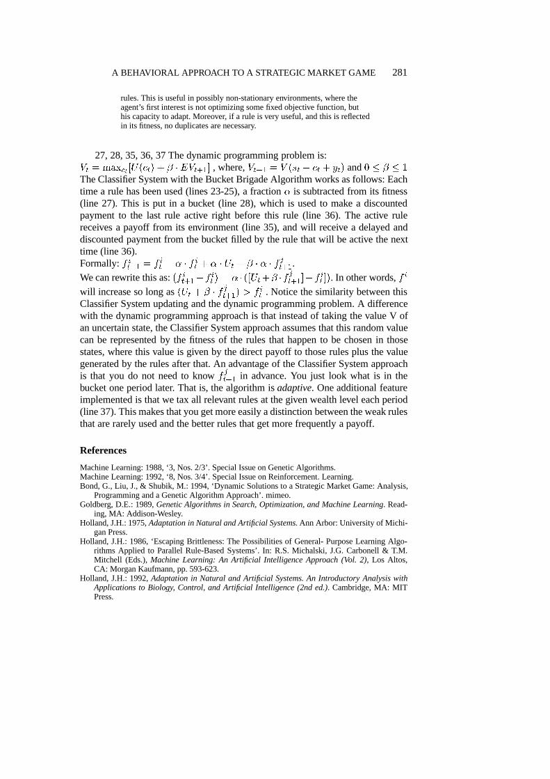
27, 28, 35, 36, 37 The dynamic programming problem is:Vt = maxct [U(ct) + � �EVt+1] , where,Vt+1 = V (st � ct + yt) and0 � � � 1

The Classifier System with the Bucket Brigade Algorithm works as follows: Eachtime a rule has been used (lines 23-25), a fraction� is subtracted from its fitness(line 27). This is put in a bucket (line 28), which is used to make a discountedpayment to the last rule active right before this rule (line 36). The active rulereceives a payoff from its environment (line 35), and will receive a delayed anddiscounted payment from the bucket filled by the rule that will be active the nexttime (line 36).Formally:f i

t+1 = f it � � � f i

t + � � Ut + � � � � fjt+1.

We can rewrite this as:(f it+1�f i

t ) = � � ([Ut+� �fjt+1]�f i

t ]). In other words,f i

will increase so long as(Ut + � � fjt+1) > f i

t . Notice the similarity between thisClassifier System updating and the dynamic programming problem. A differencewith the dynamic programming approach is that instead of taking the value V ofan uncertain state, the Classifier System approach assumes that this random valuecan be represented by the fitness of the rules that happen to be chosen in thosestates, where this value is given by the direct payoff to those rules plus the valuegenerated by the rules after that. An advantage of the Classifier System approachis that you do not need to knowf j

t+1 in advance. You just look what is in thebucket one period later. That is, the algorithm isadaptive. One additional featureimplemented is that we tax all relevant rules at the given wealth level each period(line 37). This makes that you get more easily a distinction between the weak rulesthat are rarely used and the better rules that get more frequently a payoff.

References

Machine Learning: 1988, ‘3, Nos. 2/3’. Special Issue on Genetic Algorithms.Machine Learning: 1992, ‘8, Nos. 3/4’. Special Issue on Reinforcement. Learning.Bond, G., Liu, J., & Shubik, M.: 1994, ‘Dynamic Solutions to a Strategic Market Game: Analysis,

Programming and a Genetic Algorithm Approach’. mimeo.Goldberg, D.E.: 1989,Genetic Algorithms in Search, Optimization, and Machine Learning. Read-

ing, MA: Addison-Wesley.Holland, J.H.: 1975,Adaptation in Natural and Artificial Systems. Ann Arbor: University of Michi-

gan Press.Holland, J.H.: 1986, ‘Escaping Brittleness: The Possibilities of General- Purpose Learning Algo-

rithms Applied to Parallel Rule-Based Systems’. In: R.S. Michalski, J.G. Carbonell & T.M.Mitchell (Eds.),Machine Learning: An Artificial Intelligence Approach (Vol. 2), Los Altos,CA: Morgan Kaufmann, pp. 593-623.

Holland, J.H.: 1992,Adaptation in Natural and Artificial Systems. An Introductory Analysis withApplications to Biology, Control, and Artificial Intelligence (2nd ed.). Cambridge, MA: MITPress.


Karatzas, I., Shubik, M., & Sudderth, W.D.: 1992, ‘Construction of Stationary Markov Equilibriain a Strategic Market Game’. Working Paper 92-05-022, Santa Fe Institute.

Karatzas, I., Shubik, M., & Sudderth, W.D.: 1995, ‘A Strategic Market Game with Secured Lend-ing’. Working Paper 95-03-037, Santa Fe Institute.

Lettau, M., & Uhlig, H.: 1996, ‘Rules of Thumb versus Dynamic Programming’. mimeo.Lin, L.J.: 1992, ‘Self-Improving Reactive Agents Based on Reinforcement Learning, Planning and

Teaching’.Machine Learning8, 293-321.Miller, J.H., & Shubik, M.: 1992, ‘Some Dynamics of a Strategic Market Game with a Large Num-

ber of Agents’. Working Paper 92-11-057, Santa Fe Institute.Sutton, R.S.: 1992, ‘Introduction: The Challenge of Reinforcement Learning’.Machine Learning

8, 225-227.Vose, M.D.: 1991, ‘Generalizing the Notion of Schema in Genetic Algorithms’.Artificial Intelli-

gence50, 385-396.

Date post:	19-Mar-2022
Category:	Documents
Upload:	others
View:	2 times
Download:	0 times

A BEHAVIORAL APPROACH TO A STRATEGIC MARKET GAME 1

Documents