Page 1
A Bi-Objective Tactical Planning Model for the Reverse Supply Chain
of
Durable Products
Amir Khajavi Bajestani
A Thesis
In the Department
of
Mechanical and Industrial Engineering
Presented in Partial Fulfillment of the Requirements
For the Degree of
Master of Applied Science (Industrial Engineering) at
Concordia University
Montreal, Quebec, Canada
June 2013
“©Amir Khajavi Bajestani, 2013”
Page 3
iii
Abstract
A Bi-Objective Tactical Planning Model for the Reverse Supply Chain Of
Durable Products
Amir Khajavi Bajestani
Recent environmental legislations and customer awareness on environmental impacts of landfill
activities as well as the profitability of reverse supply chains (RSC) have drawn the attention of
researchers and companies to RSC management. RSCs include the series of activities from acquiring
a used product until its recovery and sending it back to the market. In this thesis, we propose an
integrated RSC tactical planning model under the context of complex durable products. The durable
products consist of various types of components. This attribute makes them subject to the all
disposition options including remanufacturing, part harvesting, material and bulk recycling. The
proposed model decides on the coordinated decisions on acquisition, disassembly, grading, and
disposition activities in the reverse supply chain. Unlike the majority of works in the literature, our
contributions include two objective functions addressing both financial and environmental criteria.
Furthermore, we also consider two quality levels for returns, as well as a multi-indenture structure
for the end-of-life (EOL) products, and consequently all possible recovery options in the RSC. We
formulate the problem as a bi-objective, multi-period mixed integer linear programming (MILP)
model. We applied the proposed model to an academic case study in the context of an EOL
electronic device. The bi-objective model is solved by the aid of the epsilon constraint method and a
set of non-dominated solutions are provided. Finally, we conduct a set of sensitivity analysis tests for
each objective function in order to determine the most significant parameters that affect the financial
and environmental criteria in this problem.
Keywords: Reverse supply chain; remanufacturing; production planning; durable products, bi -
objective optimization; epsilon-constraint method.
Page 4
iii
Acknowledgments
I would like to express my sincere appreciation and gratitude to Dr.Masoumeh Kazemi
Zanjani for her memorable trust and confidence in nominating me as her student. She is
not only an excellent supervisor but also a wonderful human being. I am much indebted
to Dr.Masoumeh Kazemi Zanjani for her supervision, recommendations and patient
feedbacks during each stage of this thesis.
I profoundly thank my parents, my sister and my brother-in-law. I have been blessed with
a supportive father and a lovely mother that although they are miles away, their love and
dedication have enabled me to reach to this educational level.
Page 5
iv
Table of Contents
List of Tables .................................................................................................................... vii
List of Figures .................................................................................................................. viii
Chapter 1 Introduction ........................................................................................................ 1
1.1 Foreword .............................................................................................................. 1
1.2 Goal of the study .................................................................................................. 3
1.3 Research contribution ........................................................................................... 5
1.4 Thesis outline ....................................................................................................... 6
Chapter 2 Literature review ................................................................................................ 7
2.1 Introduction .......................................................................................................... 7
2.1.2 Supply chains ............................................................................................... 7
2.1.3 Closed-loop and reverse supply chains ......................................................... 9
2.2 Current literature ................................................................................................ 10
2.2.1 Acquisition planning ................................................................................... 10
2.2.2 Grading and disposition planning ............................................................... 13
2.3 Conclusion .......................................................................................................... 20
Chapter 3 Problem definition and model formulation ...................................................... 22
3.1 Problem description............................................................................................ 22
3.1.1 Product features .......................................................................................... 22
3.1.2 Reverse supply chain characteristics .......................................................... 24
Page 6
v
3.2 Problem formulation .......................................................................................... 27
3.2.1 Mathematical model.................................................................................... 29
3.2.2 Objective functions ..................................................................................... 29
3.2.3 Constraints .................................................................................................. 30
3.3 Solution approach ............................................................................................... 36
Chapter 4 Case study and computational experiment ....................................................... 39
4.1 Case study .......................................................................................................... 39
4.1.2 Problem data ............................................................................................... 39
4.2 Numerical results................................................................................................ 44
4.2.1 Experimental details.................................................................................... 44
4.2.2 Epsilon-constraint method results .............................................................. 44
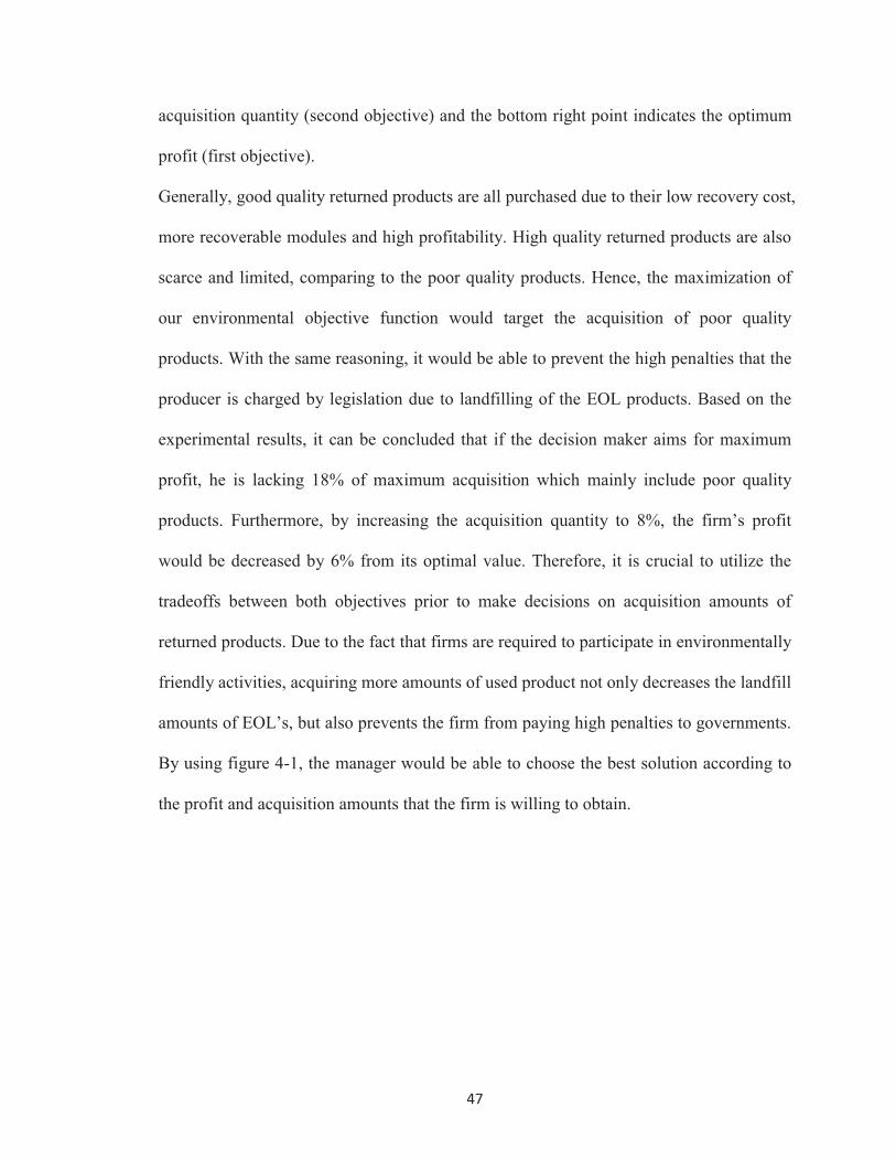
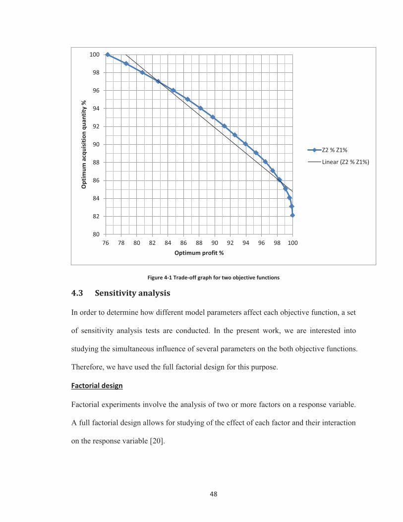
4.2.3 Analysis of the results ................................................................................. 46
4.3 Sensitivity analysis ............................................................................................. 48
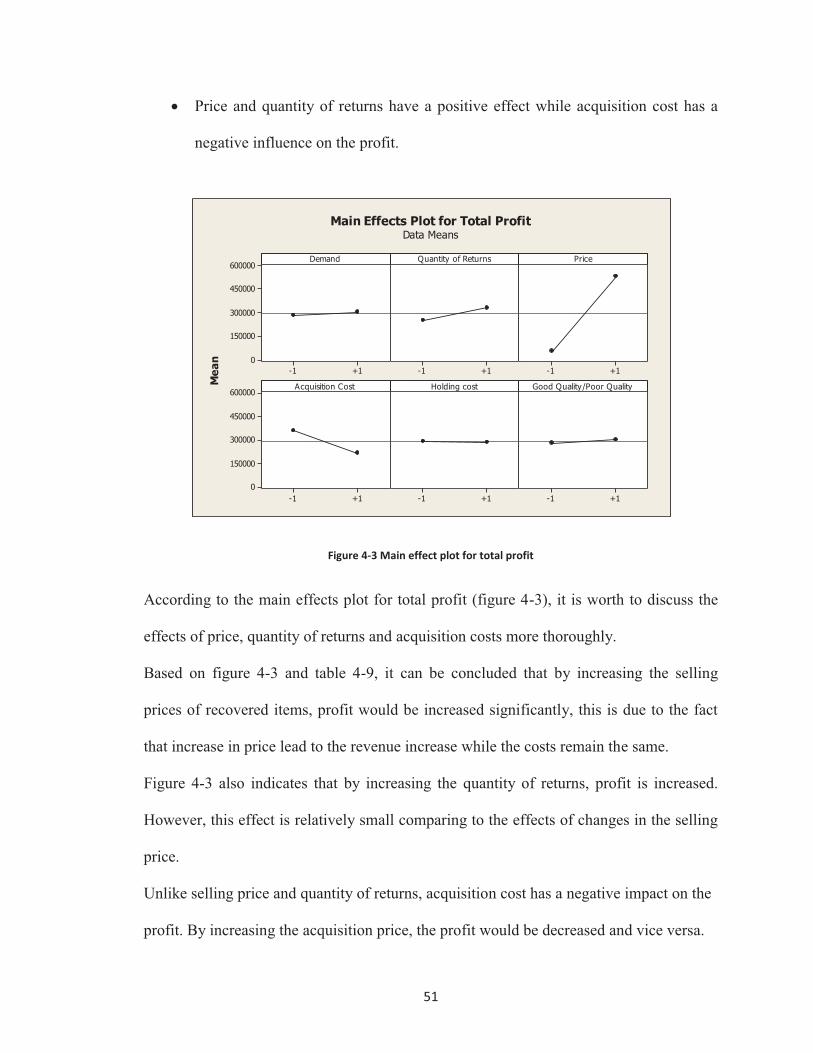
4.3.1 Sensitivity analysis on the financial objective function- Profit
maximization............................................................................................................. 49
4.3.2 Sensitivity analysis on the environmental objective function- acquisition
amount maximization................................................................................................ 56
Chapter 5 Conclusions and future research ...................................................................... 60
5.1 Conclusion .......................................................................................................... 60
5.2 Future research ................................................................................................... 63
Page 7
vi
Refrences........................................................................................................................... 65
Appendix I ........................................................................................................................ 68
Page 8
vii
List of Tables
Table 2-1 Characteristics of the closed-loop supply chains in the current literature ........ 19
Table 3-1 Decision variables ............................................................................................ 27
Table 3-2 Pay-off table ..................................................................................................... 38
Table 4-1 Number of returns for each quality levels of returned products ....................... 40
Table 4-2 The number and weights of parts and modules (BOM) ................................... 41
Table 4-3 Mass of residues, materials and disposal after disassembly ............................. 41
Table 4-4 Selling prices .................................................................................................... 42
Table 4-5 Harvesting costs................................................................................................ 42
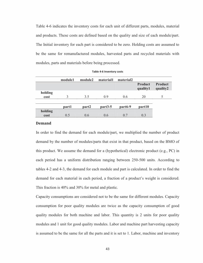
Table 4-6 Inventory costs.................................................................................................. 43
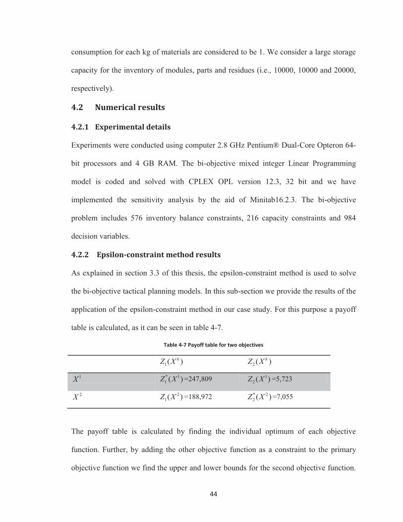
Table 4-7 Payoff table for two objectives ......................................................................... 44
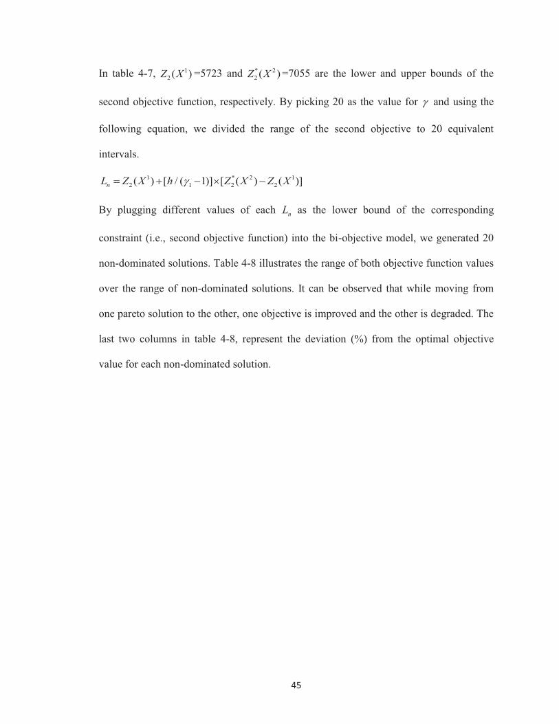
Table 4-8 Payoff table for gamma=20 .............................................................................. 46
Table 4-9 ANOVA table for profit ................................................................................... 50
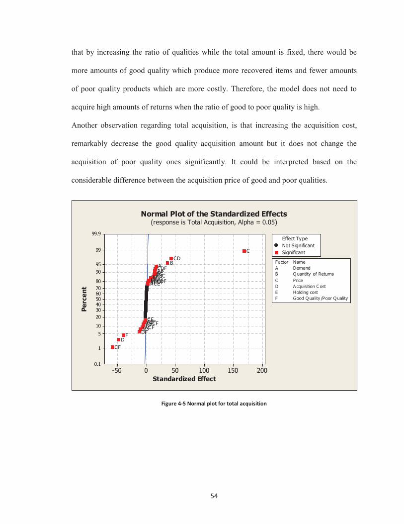
Table 4-10 ANOVA table for total acquisition................................................................. 55
Page 9
viii
List of Figures
Figure 3-1 Modular structure of a durable product ........................................................... 24
Figure 3- 2 Reverse supply chain configuration ................................................................ 26
Figure 4-1 Trade-off graph for two objective functions ................................................... 48
Figure 4-2 Normal plot of the effect on Total profit ......................................................... 50
Figure 4-3 Main effect plot for total profit ....................................................................... 51
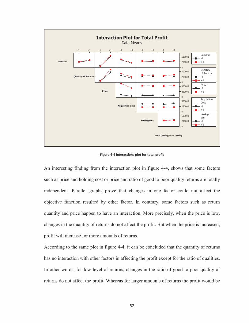
Figure 4-4 Interactions plot for total profit ....................................................................... 52
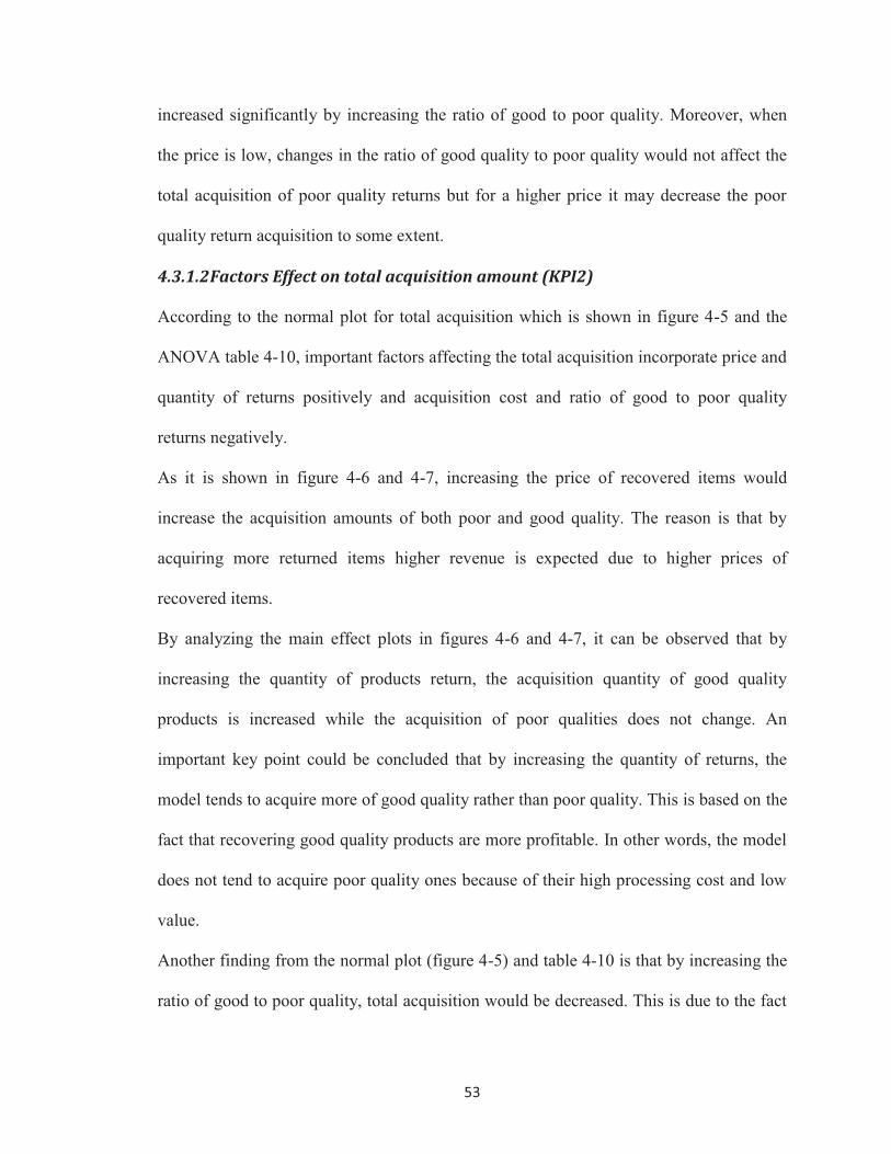
Figure 4-5 Normal plot for total acquisition ..................................................................... 54
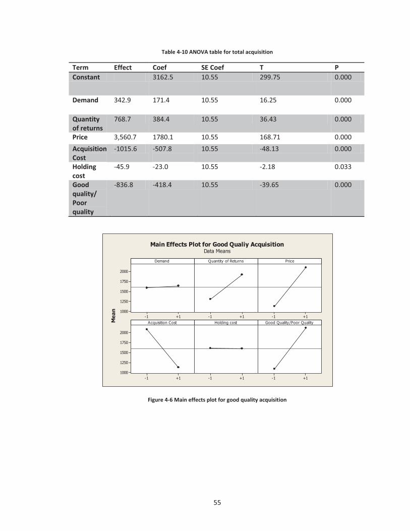
Figure 4-6 Main effects plot for good quality acquisition ................................................ 55
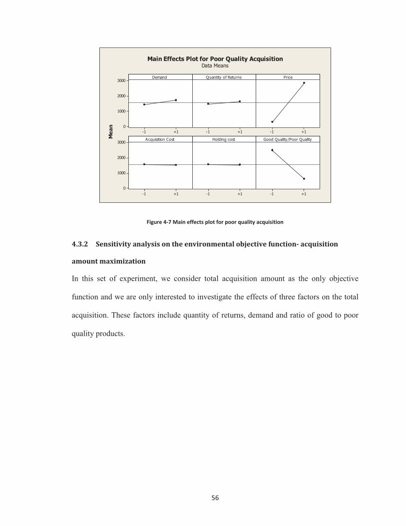
Figure 4-7 Main effects plot for poor quality acquisition ................................................. 56
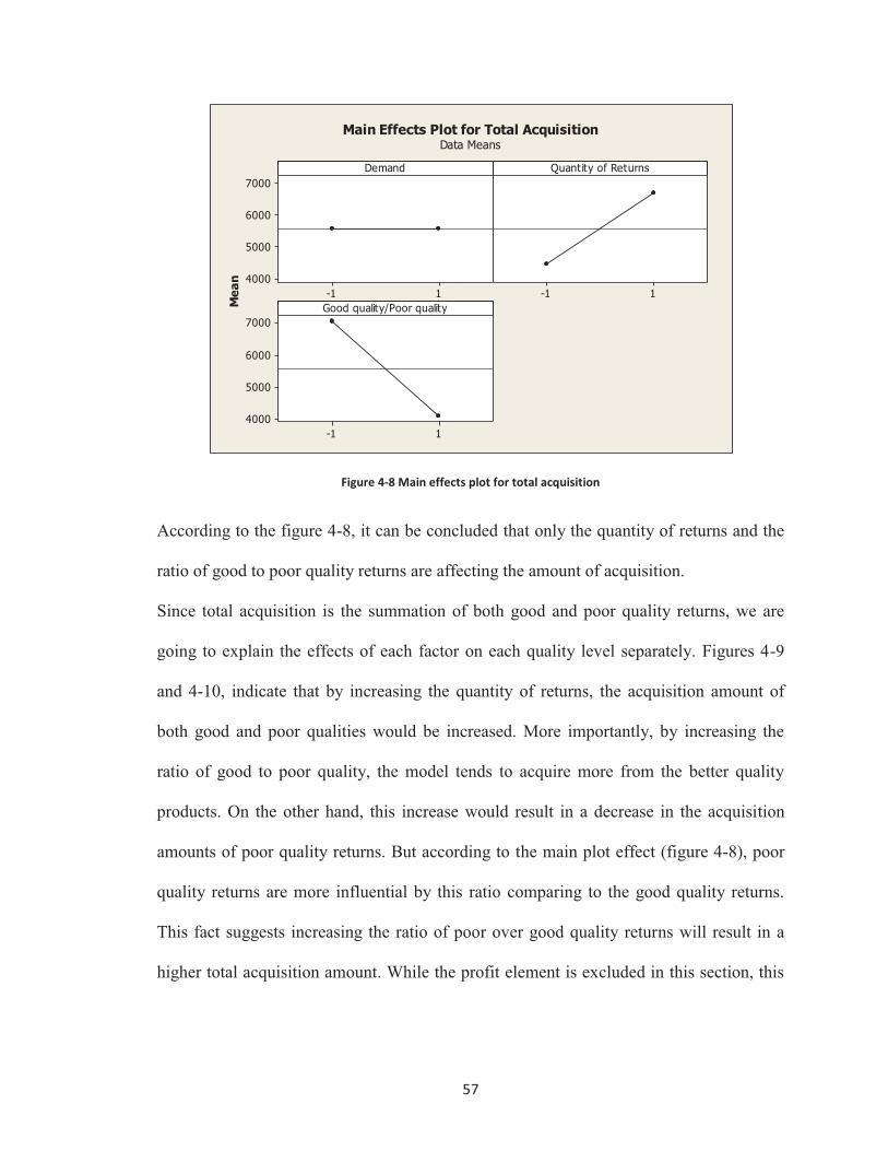
Figure 4-8 Main effects plot for total acquisition ............................................................. 57
Figure 4-9 Main effects plot for good quality acquisition ................................................ 58
Figure 4-10 Main effects plot for good quality acquisition .............................................. 58
Figure 4-11 Interaction plot for total acquisition .............................................................. 59
Page 10
1
Chapter 1 Introduction
1.1 Foreword
During a United Nations conference on human environment in 1972, in which developed
and developing nations had been gathered to discuss the preservation and enhancement of
the human environment, the concept of sustainability was brought out. The concept has
been further developed to the point that a global consciousness regarding the
environmental issues such as earth, natural resources and human life threats has been
aroused [18]. This awareness has been enforced recently by government’s participation in
the sustainable development. Therefore, new legislations are enacted that require
producer’s responsibility of their waste and emission to achieve environmental
sustainability. Many European countries created a system, called ERP (Extended
Producer Responsibility), by which the producers require to take-back, recycle and
dispose their end-of-life (EOL) products.
Sustainability includes three pillars: 1) environmental, 2) social and 3) economical ones.
Firms’ contribution could be along the three mentioned pillars by increasing the profit
generated and decreasing the environmental and social footprints. As the result, closed
loop supply chains (CLSC), has drawn the attention of researchers and companies. In the
reverse side of CLSC’s, environmental responsibilities could be met by the recovery of
EOL products and diverting them from landfill to reuse. Products are the source of
environmental issues, because in order to create a product, natural resources are
consumed, manufacturers’ machineries exhaust and pollute water and earth. Eventually
the EOL products could damage the environment by leaving their hazardous and non-
hazardous compounds on the earth.
Page 11
2
Socially wise, green activities help the producer to build a good creditability among the
consumers who reasonably expect them to eliminate their environmental harm. Another
advantage of the EOL recovery practices is the Profitability and the value generated by
the firms. Producing a brand new unit of product is always more expensive than
remanufacturing it. Moreover, by remanufacturing, many parts and components could be
reused, therefore resources would be preserved. Further, upon reuse, firms are extending
the product’s life cycle by keeping them out of landfill [14].For instance, over the last
decade Kodak has recycled more than 310 million single-cameras in more than 20
countries [16].
According to the above mentioned advantages, reverse supply chains are becoming an
essential part of businesses, among which the OEMs (original equipment manufacturers)
of automotive parts, cranes and forklifts, furniture, medical equipment, pallets, personal
computers, photocopiers, telephones, televisions, tires, and toner cartridges are ahead of
others [14]. Recovering the EOL products could vary significantly from one industry to
another. This deference roots back to the nature of the products. Some products, such as
sand and paper are simple and they do not contain hazardous materials. On the other hand,
complex products such as electronic wastes consist of a considerable amount of materials
and parts, some of which are hazardous. Also, the recovery of such components in the
underlying industry is expected to be profitable. Therefore, maintaining an efficient and
effective reverse supply chain system is the key factor that gives the firm the ability to
succeed and stay competitive in the market, both financially and environmentally.
Reverse supply chain includes the series of activities from acquiring a used product until
recovering and sending it back to the consumer market. In the process of a typical RSC to
Page 12
3
recover a complex product, such as an electronic waste core, there are several key
decisions involved, namely product acquisition, grading (inspection), and disposition,
including disassembly, remanufacturing, recycling, part harvesting, and disposal.
Regarding the acquisition, firms could passively accept all returned items or exert control
over the acquired products through acquisition decisions [16]. Grading decisions are
directly influenced by the acquisition policies. When the firms accept all the returns
without exerting control over the quality levels of returns, the evaluation responsibility
burden the grading center. Generally, grading unit is the link between acquisition and
disposition decisions. The Disposition problem can be defined as “a given set of cores
and a set of available recovery options” [24].
In order to have an efficient RSC, an integrated tactical planning to combine all the
sections in the above mentioned RSC is required. Another important aspect is raised from
the environmental viewpoint, in which by acquiring more of EOLs, firms would be able
to prevent the waste placement into the landfill. Thus, first as a social result, a good
public reputation would be built up based on the fact that companies are environmentally
friendly. And second, it helps the manufacturer financially because if the OEMs fail to
take back a certain amount of their products, they will end up paying high penalties.
1.2 Goal of the study
The goal in the underlying study is to propose an integrated tactical planning tool in a
RSC corresponding to durable products. Durable products, such as computers, mobile
phones, copy machines, washing machines and automobiles, require to be treated
differently than other wastes such as papers, containers, etc. EOL durable products are
distinguished by their high recoverable value and long product life cycle. They often
Page 13
4
consist of multiple and various types of components. The specific characteristic of
durable products rises to the challenge of choosing a proper RSC setting. In this context,
our reverse supply chain consists of different facilities, such as collection, disassembly
and inspection, disposition and redistribution. We are also interested to integrate all the
reverse supply chain tactical-level decisions. In other words, we aim for integrating all
the tactical level decisions from collecting the EOL to selling the recovered items to the
market. Demand is estimated over a multiple period setting, and returns are assumed
belonging to two different quality levels, good and poor qualities, where the proportion is
known in advance. The tactical level decisions in this study correspond to a complete
bill-of-material of a durable product in electronic industry and include all the possible
recovery options. The decision variables in each period in the planning horizon are as
follows:
� Number of products of different quality levels purchased and disassembled.
� Number of modules and parts to remanufacture and harvest.
� Mass of each material to recycle.
� Inventory of products, modules, parts, materials, residues and disposal.
� Sales amount of recovered modules, parts and materials.
To formulate the underlying problem mathematically, a MILP (mixed integer
programming model) is proposed that includes two objective functions: 1) financial and 2)
environmental ones. According to the current literature, most of the researchers and firms
try to maximize their profit (or minimize the cost), but the environmental criteria is
seemed to be overlooked from the common practice. Investigating the solution of two
objective functions is a challenge, given the fact that our financial and environmental
Page 14
5
objectives are in conflict. Therefore, there is a need to find a set of “most-preferred”
solutions by the aim of multi-objective optimization methods. In this study we apply the
epsilon-constraint method to find a pareto-front for the trade-off between the two
objective functions.
Finally, we also conduct a set of sensitivity analysis tests for each objective function in
order to determine the most significant parameters that affect the financial and
environmental criteria in this problem.
1.3 Research contribution
According to the literature, the majority of works that have been done in the context of
RSC tactical planning only addressed the financial aspects of the problem (profit
maximization/cost minimization) and they failed to consider the minimization of negative
environmental impacts, although RSC activities, target the reduction of environmental
footprint by its nature. Furthermore, considering the most possible recovery options and
different quality levels of EOL returns are other shortcomings of the current contributions
in the literature.
The key considerations in this study that contribute to the existing literature are as
follows:
� An integrated tactical planning model including acquisition, grading and
disposition (remanufacturing, harvesting, recycling and disposal) decisions in the
context of a durable product RSC proposed.
� A multi-indenture structure is considered for the EOL products. Consequently, all
possible recovery options are taken into account.
� Two objective functions addressing both financial and environmental criteria are
Page 15
6
proposed.
� Two quality levels for returns are considered. They differ in the acquisition price,
recovery and processing costs, and the amounts of recoverable components.
This study contributes to a valid and strong tool for researchers and practitioners in the
RSC related fields. The tactical planning model proposed in this thesis is applicable in the
durable products context. Since sustainability is a fairly new concept and most companies
seem to be unaware of their environmental footprint, by the aim of this tool companies
will be able to increase their profit while eliminating their environmental footprint.
1.4 Thesis outline
Following the introductory chapter, a literature review is provided in chapter 2. In chapter
3, problem description, model formulation and solution methodology are presented.
Chapter 4 includes our case study and the experimental results. Finally, conclusions and
recommendations for future contributions are discussed in chapter 5.
Page 16
7
Chapter 2 Literature review
2.1 Introduction
Profitability and the value generated by reverse supply chains (RSC), as well as recent
increase in legislations and customer awareness on environmental impacts of landfill
activities have drawn the attention of researchers to RSC’s management. Environmental
responsibilities could be met through improving the recovery of end-of-life (EOL)
products and diverting them from landfilling to reuse which is the main motivation of
RSC management. According to the growing concerns, the producers need to take
advantage of practicing in closed loop and reverse supply chains. In this chapter, relevant
literature of reverse supply chains is discussed. Prior to describe the current literature, we
briefly review the features of supply chains and RCS’s, as follows:
2.1.2 Supply chains
A supply-chain encompasses all activities associated with the flow of goods from
acquiring the raw material, adding value through manufacturing, and delivering the final
goods to the end user. There are five entities in every supply chain: 1) raw material
suppliers, 2) manufacturers, 3) wholesalers/distributors 4) retailers, and 5) customers. The
objective of every supply chain could be seen from different perspectives, but the
consensus is to maximize the overall value generated. This value is the difference
between what the final product worth to the customer and the costs that supply chain
incurs in filling the customer’s request. This generated value is a measure of profitability.
The higher the supply chain profitability is, the more successful the supply chain would
be [15].
Page 17
8
Successful supply chain management requires making many decisions relating to the
flow of information, product, and funds. According to Chopra and Meindl [15], these
decisions fall into three basic categories in which we consider activities over specific
time horizon. These categories are as follows:
1) Supply chain strategic planning: during this phase company decides how to structure
and design the supply chain over a long period of time (years). The decisions are mainly
focused on the location and capacity of the production, and the warehousing facilities, the
quantity of products to be manufactured and stored at various locations, the mode of
transportation and the type of information system to be utilized. These decisions are long
term and are very expensive to change.
2) supply chain tactical planning: The time frame considered in SC tactical planning is a
quarter to a year. Company decides on medium-term decisions, such as procurement
planning, supplier selection, production, inventory and distribution planning. Given a
shorter time frame and better forecasts than the design phase, companies in the tactical
planning level, try to incorporate any flexibility built into the supply chain in the design
phase, and exploit it to optimize performance.
3) Supply chain operation planning: these decisions are short-term (daily or weekly)
plans. Companies make decisions regarding individual customer orders, allocating
inventory or production to individual orders, set a date that an order is to be filled,
generate pick lists at a warehouse, set delivery schedule of trucks and place
replenishment orders. Given a shorter time frame than the tactical planning phase, the
goal is to exploit the reduction of uncertainty and optimize performance.
Page 18
9
2.1.3 Closed-loop and reverse supply chains
Reverse supply chains are supply chains where in addition to the typical forward flow of
materials from suppliers to the end customers, there are flows of products back to
manufacturers [14]. A reverse supply chain network begins with the collection of used
products from end-user. According to Aras et al. [17], there are different structures of the
reverse supply chains in practice, and the nature of the used product and the type of
recovery activity play an important bearing on the structure of the RSC. However,
collecting or acquisition, grading and disposition decisions are the major elements of a
RSC.
Product acquisition activities represent the supply side of CLSCs and include feeding the
products back into the supply chain [24]. There are two types of acquisition systems,
market-driven and waste-stream. In the market-driven case, firms exert control over the
quality of acquired items via different methods. This control could be through pricing
decisions. In a waste-stream system, firms accept all the returns without exerting careful
control over the quality levels of returns, therefore the role of acquisition management is
not significant. In this situation, the focus is more on the grading activities after
acquisition. In the grading activities, the used products are evaluated and tested for proper
recovery decisions. Different grading methods exist in order to define the quality status of
products. Once the quality of products is known they are classified for further treatments.
The objective is to optimize the performance by determining the right grading decisions.
The grading unit is the link between acquisition and disposition activities. After grading,
a RSC is faced with multiple options for further treatment depending on the type of the
products. These decisions are recalled as disposition decisions. The disposition problem
Page 19
10
is straightforward for a single core, but when disassembling a product yields multiple
components, a good disposition decision has to take into account all of these components
and seek global optimum among them. The simplest form of disposition decision for a
core is the choice of remanufacturing and disposal [24]. However for a more complex
product, this could be a combination of remanufacturing, refurbishing, recycling, part
harvesting, land filling, incineration, internal reuse, and resale. Remanufacturing or
refurbishing is the highest profitable, and at the same time the most costly recovery
activity among the disposition options. Remanufacturing includes disassembly, cleaning,
repairing, replacing parts and reassembly and consists of bringing the used product to a
common operating and aesthetic standard [25]. Refurbishing is defined as ‘light’
remanufacturing and it include a minor disassembly. The parts recovery includes cleaning
and repairing a used part in order to reuse it. Incineration could be used to reduce the
landfill amount and energy recovery, however there exist some disadvantages such as
emission and pollution in the incineration practices. Resale and reuse refer to activities
where there is no need for treatment and the equipment could be used as-is.
A comprehensive literature on the aforementioned elements of RSC’s are described as
follows.
2.2 Current literature
In this section, we briefly review the existing literature on acquisition, grading, and
disposition planning in reverse and closed-loop supply chains, as follow.
2.2.1 Acquisition planning
Guide and Van Wassenhove [16] stated that firms could passively accept all returned
items or exert control over the acquired products through acquisition decisions. Different
Page 20
11
works in this regard have been done. Some addressed the optimal acquisition price
regardless of different quality levels of returns [19-22], while others discussed a situation
where manufacturer must grade the collected items to effectively manage the quality
variability [2-4].
Robotis et al. [3], studied the effect of remanufacturing on procurement decisions for
resellers in the secondary markets. At first, it is assumed that the reseller procures used
products from two classes of suppliers and after sorting them, she sells those products
whose quality is higher than the acceptable quality level for that class, and then disposes
off the rest. In the proposed model framework, the reseller observes the quality of
returned products and decides to remanufacture some of them. They have considered two
quality levels of products and the objective is to maximize the profit. They concluded that
using remanufacturing to serve secondary markets reduces the number of units procured
from the suppliers and it is always better to use remanufacturing to a certain extent. They
also showed that by using remanufacturing, resellers can eliminate some of their
suppliers who may be providing items of low quality.
Atasu and cetinkaya [1] presented a RSC study on lot sizing and optimal collection and
use of remanufactruable returns over a finite life-cycle. They considered a setting where a
collector obtains used product at a constant return rate. The collector then, ships these
returns to the manufacturer regularly. Since all remanufactured products are substitutable
for satisfying the demand for new products, the manufacturer would like to cover demand
using as many remanufactured products as possible. The model concentrates on the case
where a single production lot of new items are produced by the manufacturer early in the
active market demand period. They also provided a method for making better use of
Page 21
12
returns by taking advantage of their time value in the manufacturer-collector
collaboration.
Zikopolous and Tagaras [4] investigated the impact of uncertainty in the quality of
returns on the profitability of a RSC. They developed a stochastic programming model
for a single-period reverse supply chain planning. The underlying reverse network
includes two collection facilities and one refurbishing site. Returns are conveyed to the
refurbishing facility from two collection sites. The authors took into account two
different uncertain quality levels of returns such that qualities are revealed only after
being received by the refurbishing center. The uncertainty in quality of returns is
considered as a continuous random variable. Returned units are sorted upon arrival to the
refurbishing facility and disposed if they do not meet the quality standards for
refurbishing. Refurbished items are sold to the market. The demand for the refurbished
items is assumed to be continuous random variables. The problem in this study contains
three decision variables, including the quantities to transport from each collection site to
the refurbishing center and the quantity to be refurbished. The objective function is to
maximize the expected profit. They concluded that the quality of returns has a significant
effect on the profitability of the reverse supply chain. Furthermore, they proposed
splitting the total procurement quantity between the two collection sites is beneficial to
the system.
Galbreth and blackburn [2] studied the optimal acquisition quantities in remanufacturing.
The remanufacturer should decide on the quantity of used items to acquire for
remanufacturing and the quantity to scrap. These used items are classified into different
quality levels which are widely varying and uncertain. The condition variability was
Page 22
13
described by a continuum as well as two discrete categories of remanufacturable used
items. Acquiring higher volume of used products results in having more of better quality
products and therefore remanufacturing costs would decrease, but this reduction in cost
would incur higher acquisition cost. Hence, in this work, the tradeoff between acquisition,
scrapping and remanufacturing costs is examined. The objective was to minimize the
total cost. Data were taken from a cell phone remanufacturer. They concluded that when
costs are linear, the optimal acquisition quantity has a closed form and increases with the
square root of the degree of condition variability.
2.2.2 Grading and disposition planning
Black burn et al. [23] discussed the appropriate location of grading operations, in term of
testing returns at the centralized and decentralized facilities. Guide et al. [19] proposed an
analytical model to quantify the trade-offs in the grading location decisions. Denizel et al.
[5] investigated a remanufacturing environment where returns are graded and grouped
into a number of different quality levels. A promising work in the closed loop supply
chain is done by Sheu et al. [10]. In this work, an integrated logistics operational model
for green supply chain management was proposed. A linear programming model was
formulated to optimize the operations of both integrated forward and reverse logistics in a
green-supply chain. Their comprehensive framework is classified into manufacturing
supply chain and used-product reverse supply chain. The manufacturing supply chain
includes raw material supply unit, manufacturing facility, whole sale unit, retailing and
end-customers. Similarly, the reverse supply chain consists of collection centers,
recycling plants, disassembly plants, secondary material markets and final disposal
locations of wastes. The objective is to find equilibrium solution to maximize the net
Page 23
14
profit for the both forward and reverse supply chain. For the numerical study a real case
of notebook computer manufacturer was considered. Their findings showed that, in an
integrated forward-reverse supply chain, increased profit from the reverse supply chain is
relatively small compared to the forward manufacturing chain. However, reverse supply
chains can be benefited from the governmental subsidy policies and ultimately lead to
prevention of environmental legislation expenses.
Sodhi and Reimer [11] presented a model for RSC of recycling EOL electronics. In the
proposed model, the reverse channels for the recycling of electronics are represented as a
network of flow between generators, recyclers and material processors. The recyclers
collect electronics waste from different sources and manufacturers. Then, through further
processes, such as disassembly and separation, products are broken down to different
parts and components. From there, they are forwarded to smelters to process into pure
stream of metal and plastics. A typical electronics recycling network includes three
processing units, mixed material sources, recyclers and smelters. Linear mathematical
models were formulated to optimize the profit for each processing unit, separately. At the
recycler’s level, an integrated disassembly and material recovery problem was formulated.
Jayaraman [9] addressed production planning for closed-loop supply chains with product
recovery and reuse options. In this framework, first, products are returned from the end
users. Once the products are returned, there are several options to treat them such as sell,
clean and repair, refurbish and sell, remanufacture, retrieve valuable parts, recycle and
disposal. It is profitable to employ all of the mentioned treatment options except disposal,
which has to be minimized or eliminated. The profitability of such systems also depends
on the ability to minimize the environmental impact of used products. They assumed the
Page 24
15
incoming products have different quality levels. Decision variables in their model include
the number of unit cores acquired in each period, the number of unit core disassembled in
each period, the number of unit cores and modules remanufactured in each period, the
number of unit cores and modules disposed in each period, and the number of cores,
modules and remanufactured cores, remaining in the inventory at the end of each period.
A linear programming model was formulated to minimize the total cost of the reverse
supply chain in a multi period setting. They collected the data from a cellular phone
manufacturer for their case study. It was concluded that the acquisition price affects the
acquisition quantity of used products.
Walther and Spengler [12], examined the impacts of waste electrical and electronics
equipment (WEEE) directives on reverse logistics in Germany. The adoption of these
directives causes essential changes in the field of electronic scrap recycling. Hence, they
developed a mixed integer optimization model for integrated disassembly and recycling
planning to predict relevant impact of the legislations on the treatment of discarded
electronic products. The decision variables include the masses of products to acquire,
masses of products or disassembly fraction accepted from another disassembly company,
number of executions of disassembly activities and masses of disassembly fraction
delivered to recycling or disposal site. The objective is to maximize annual marginal
income of the network. The data were collected from a real case study in entertainment
electronics in Germany. Some of their findings include that by increasing centralization
tendencies, transportation costs and thus emissions will rise which contradicts the
sustainability practices, therefore small companies need to cooperate and bundle
Page 25
16
capacities and acquisition processes. Joint utilization of vehicles and joint investments in
vehicles with higher capacity are other possibilities for network cooperation.
Ferguson et al [6] investigated the value of grading in remanufacturing. They considered
a tactical production planning problem in a remanufacturing firm. In this study, products
are returned to the firm’s return facility. Returned products are coming from a broad
range of different quality levels. Afterward, they are graded to three different quality
levels. Grading procedure determines the proper disposition option for the product to
undergo. The decision variables are the number of products to remanufacture, the
quantity of returns to salvage and inventory of both returned and remanufactured
products. Demand is forecasted for the remanufactured products but it is considered to be
different than the demand for new products. They collected the data from a mailing
equipment manufacturer. A greedy heuristic solution algorithm was developed to solve
the problem. Based on their analysis, grading the returns would increase profit by
4 %.They proposed a number of managerial insights as follows. First, the ratio of return
rates to demand rates has a direct relation with the value of grading. Second, the major
benefits of applying a grading system in remanufacturing occur when there are no more
than five quality levels for grading.
In a comprehensive work regarding grading and disposition planning, Doh and Lee [8]
proposed a grading and production planning model in a reverse supply chain. In their
problem, the used products are collected through the collection facilities and stored at the
“collected items” inventory. Then in the grading step, they are inspected, and tested to
determine if products are remanufacturable or not. Remanufacturable products are
disassembled to parts and components and are stored in the inventory for further
Page 26
17
processing and reassembly. Non-remanufacturable products are sent to disposal units.
The decision variables are the number of products to be disassembled or disposed, the
number of parts or components to remanufacture or dispose and the number of products
to be reassembled in each period. The objective is to maximize the profit. They
formulated the problem as a mixed integer programming model. They also provided two
heuristic solution algorithms.
Kim et al [7] proposed a supply planning model for remanufacturing in a reverse logistics
network. In this framework, end-of-life products are returned to the collection facility,
then, they are disassembled and disposed to different parts. Disassembled parts are
classified into reusable and non-reusable parts. In this study, only one disposition option,
refurbishing, is considered and the products beyond the capacity are sent to external
remanufacturing subcontractors. Non-usable parts are sent to disposal. The author also
considered the possibility of obtaining some new parts from an external supplier. The
decision variables include the number of disassembled products, the number of
refurbished and disposed products in each period and the inventory level of products and
parts. Moreover the manager has to decide on the number of purchased new parts as well
as the number of outsourced products. The objective function is to maximizing the profit
and the problem was formulated as a mixed integer programming model. The data were
taken from a real case study. Sensitivity analyses were also performed to examine the
different ways of cost savings.
Denizel et al [5] proposed a multi-period remanufacturing planning model with uncertain
quality of inputs. In this model, one type of product with the uncertain quality levels is
considered. Demand is forecasted and known for different periods. They assumed that
Page 27
18
cores arrive at the firm and are graded, then after observing the outcome of the grading
process, the manager decides upon the amount to salvage and refurbish for each quality
grade. Decision variables are the number of products to grade, the graded core to
remanufacture as well as the number of cores to salvage. A multi-stage stochastic
programming model was proposed to formulate this problem. The objective function is to
maximize the total expected profit. Data were obtained from a real business case study,
namely remanufacturing mailing equipment. The authors also did a broad numerical
study and regression analysis to measure the relative impact of each parameter on profit.
Some of their findings can be summarized as follows: firm’s profit is vastly related to the
quality of the cores, the salvage value of unused products and the cost of grading.
Furthermore, most of the times it is more profitable to remanufacture all of the higher
quality cores, except when the cost of grading is high and firms have to grade and
remanufacture only enough to meet the demand.
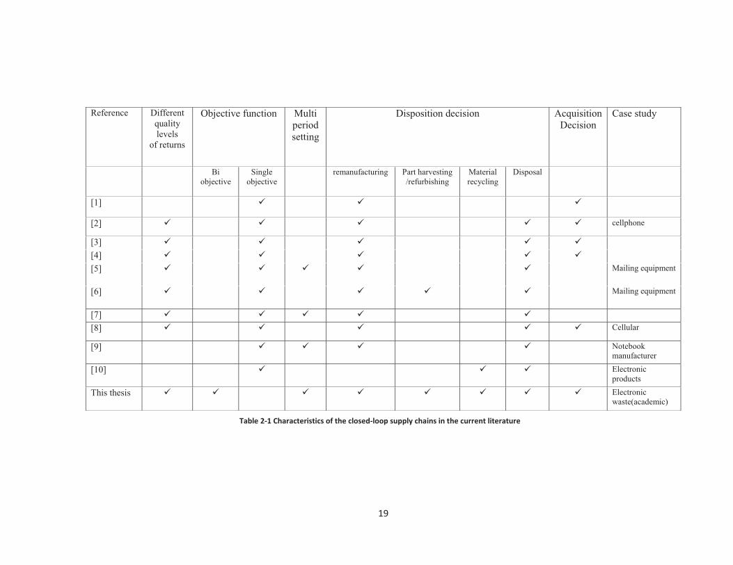
According to the literature review in this section, the characteristics of different reverse
and closed-loop supply chains studied in the literature are summarized in table1. The last
row of the table contains the features of the RSC investigated in this thesis.
Page 28
19
Reference Different quality levels
of returns
Objective function Multi period setting
Disposition decision Acquisition Decision
Case study
Bi objective
Single objective
remanufacturing Part harvesting /refurbishing
Material recycling
Disposal
[1] � � �
[2] � � � � � cellphone
[3] � � � � �
[4] � � � � �
[5] � � � � � Mailing equipment
[6] � � � � � Mailing equipment
[7] � � � � �
[8] � � � � � Cellular
[9] � � � � Notebook manufacturer
[10] � � � Electronic products
This thesis � � � � � � � � Electronic waste(academic)
Table 2-1 Characteristics of the closed-loop supply chains in the current literature
Page 29
20
2.3 Conclusion
In this chapter, we reviewed the most recent literature in the field of CLCS’s and RSC’s
tactical planning. Firms in many industries are trying to increase their activities on
reverse supply chain according to the new legislations. Existing models have tried to
capture different aspects of closed-loop and reverse supply chains. However, a clear gap
in the literature still exists according to the different structures of a CLSC or RSC. For
instance, in the content of complex product, after disassembly, different types of
components, namely, modules, parts, residues, materials and disposal would be yielded.
Therefore different types of disposition options can be considered. In contrary, when a
product is simple such as sand, paper, etc. only a limited number of disposition options
are possible. The current literature covers only a few of disposition options. For instance,
some authors have addressed only one disposition option [1], while others focused on two
or three options [1-10], nevertheless, none have investigated all of the possible
disposition options in the RSC. Secondly, another important setting to be considered in
the RSC and CLSC studies is the alignment with environmental concerns. Hence we
expect firms make an effort to acquire used-products from different quality levels in
order to reduce the environmental impacts of landfill. While one of the key
considerations to minimize the environmental impact in the RSC’s is to maximize the
acquired used-products among various qualities, to the best of our knowledge, current
literature in the RSC tactical planning only investigates the acquisition activities from the
economic perspective (profit maximization).
In the literature, it can be observed that some of the contributions developed a setting that
returns are from different quality levels. This variation in incoming quality levels are
Page 30
21
tackled by deterministic and stochastic mathematical programming approaches [2-8].
While most of the works did not study the control over acquisition quality, only a few
considered a setting with acquisition decisions of different quality levels [2-4].
Nonetheless, to the best of our knowledge, none of the available contributions considered
different quality levels in an integrated tactical planning problem in a RSC, as
investigated in this thesis.
Page 31
22
Chapter 3 Problem definition and model formulation
In this chapter, we first describe the features of the problem investigated in this thesis.
Then, we provide the problem formulation.
3.1 Problem description
In this thesis, we are focused on a RSC corresponding to durable products. Hence, we
first elaborate on the main features of such products. Then we provide the characteristics
of the corresponding RSC.
3.1.1 Product features
In the underlying research, we considered a complex durable product. Durable products,
such as computers, mobile phones, copy machines, washing machine and automobiles,
require to be treated differently than other wastes such as papers, containers, etc. EOL
durable products are distinguished by their high recoverable value and long product life
cycle. They often consist of multiple and various types of components that can be
recovered by different methods. The modular structure of the product is shown in figure
3-1. When the durable product is disassembled, it yields modules, parts, residues, some
precious materials and other hazardous and non-recoverable components. Modules are
units of products which would undergo remanufacturing. Remanufacturing is the highest
profitable and at the same time most costly recovery decision among all disposition
options. Remanufacturing include disassembly, cleaning, repairing, replacing parts and
reassembly and consists of bringing the used product to a common operating and
aesthetic standard [25]. Good quality EOL products consist of more remanufacturable
modules. On the other hand, poor quality returns include less number of
remanufacturable modules. Good quality and poor quality modules are different in terms
Page 32
23
of remanufacturing costs, as well. Poor quality modules are processed at high cost while
good qualities require low cost of remanufacturing. However, both quality levels would
be brought up to the same quality level through the remanufacturing processes. Poor
quality modules are nominated for remanufacturing at high cost or being sent to bulk
recycling. Spare parts are another sub-component of the disassembly process. These
spare parts are entities that would undergo the harvesting process if they meet certain
criteria for the harvesting. In this process, used parts are recovered to be sold in spare part
markets. Each product yields different numbers of a specific part, based on its quality
level. Good quality products yield more harvestable parts than poor quality ones. If parts
are not qualified for harvesting, they will be sent to bulk recycling. Other disassembly
outputs are materials. Materials such as plastic, iron, copper and aluminum are separated
after the product is shredded. Some materials could be easily extracted as they exist in
solid forms. But a big fraction of materials are combined with other compounds and it is
not easy to extract them through simple activities in material recycling’s unit. Therefore,
the residues remained after removing the hazardous and valuable materials from the
product are bulk recycled. In bulk recycling facilities, the remainder of the product is
shredded into flakes. Further, different separation methods based on physical properties
of materials are used to classify them into different categories of materials. For example,
metals are removed by magnets and eddy currents, plastics are separated based on
physical properties such as mass, density or particle size [11]. There exist other
techniques such as sink-float separation, air classification [26], and ultrasonic methods
[27] that could be used in this regard. Bulk recycling is relatively costly comparing to
material recycling and it can process large amounts of residues. The remainder of
Page 33
24
products with no value as well as potentially hazardous components are disposed (e.g.
landfilled).
Disassembly
Modules Parts Residues Material Hazardous components
Remanufacturable
Good quality
Poor quality
Marketable
Remanufacturing (low cost)
Bulk recycling
Material recycling
Bulk recycling
Disposal Material recycling
Material recycling Disposal
Non-recoverable components
Disposal
Remanufacturing (high cost)
Non-Marketable
Bulk recycling DisposalHarvesting
Disposal
Figure 3-1 Modular structure of a durable product
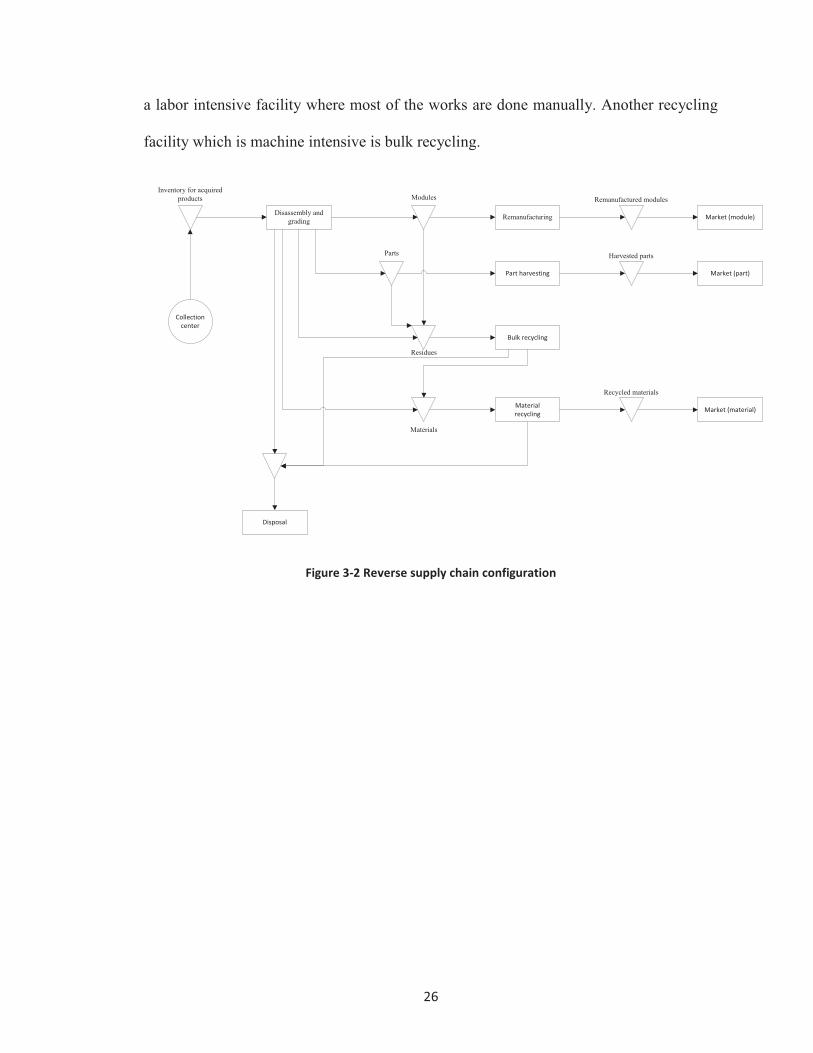
3.1.2 Reverse supply chain characteristics
Based on the features of the complex durable products, discussed previously, the
structure of our reverse supply chain is defined as follows. The reverse supply chain
includes different facilities, such as collection, disassembly and inspection, disposition
and redistribution ones. End-of-life returns are collected in the collection facility as it can
be seen in figure 3-2. These returns are assumed belonging to two different quality levels,
good and poor quality. As an example of good quality returns, we can refer to
guaranty/warranty returns. In reality, a greater percentage of these returns are from poor
quality and the rest are good qualities, as good quality EOL products are scarce and
limited. At the collection centers, the firm decides what quantity of EOL products of each
quality should be purchased in each period. Good quality products are purchased at high
price while we can acquire poor quality products at low cost and in high amount. The
Page 34
25
purchased amounts of each product are stored in the inventory of acquired products and
they are sent to disassembly facilities. All the acquired products are disassembled to their
components. Disassembly activities are mostly done manually and are labor intensive. As
mentioned before, good quality products yield more useful modules and parts rather than
poor quality products. On the other hand, more residues and consequently more materials
could be extracted from poor quality products. Disassembled outputs are inspected for
assigning to proper disposition categories. In this step, the yielded components are
categorized into the good and poor quality modules, harvestable parts, residues for bulk
recycling, recyclable materials and both hazardous and non-hazardous disposal. Each
category of items is kept in its inventory until they are transferred to their corresponding
processing facility. The model also decides if there is a need to transfer some of the low
quality modules to the bulk recycling because of the limited capacity. Remanufactured
items are raised to the same quality level and they will be sold in the market. Harvestable
parts are stored in the inventory until they are transferred to the harvesting facility.
Harvested parts are sold to the market at a lower price than the brand new parts.
According to the capacity restriction it is not possible to hold all the harvestable parts in
inventory, therefore we consider some flows to the bulk recycling from inventory of
harvestable parts. Through the disassembly process, some of the targeted materials such
as metal and plastic are removed from the product and they only need minor care and
repair, which would occur at the material recycling facility. At this facility, a fraction of
useless materials are sent to disposal facilities and the rest would be shipped to the
recycled material inventory in order to be sold in the market. Material recycling facility is
Page 35
26
a labor intensive facility where most of the works are done manually. Another recycling
facility which is machine intensive is bulk recycling.
Disassembly andgrading
Bulk recycling
Part harvesting
Remanufacturing
Material recycling
Disposal
Market (part)
Market (module)
Inventory for acquiredproducts
Market (material)
Modules
Parts
Materials
Residues
Remanufactured modules
Harvested parts
Recycled materials
Collection center
Figure 3-2 Reverse supply chain configuration
Page 36
27
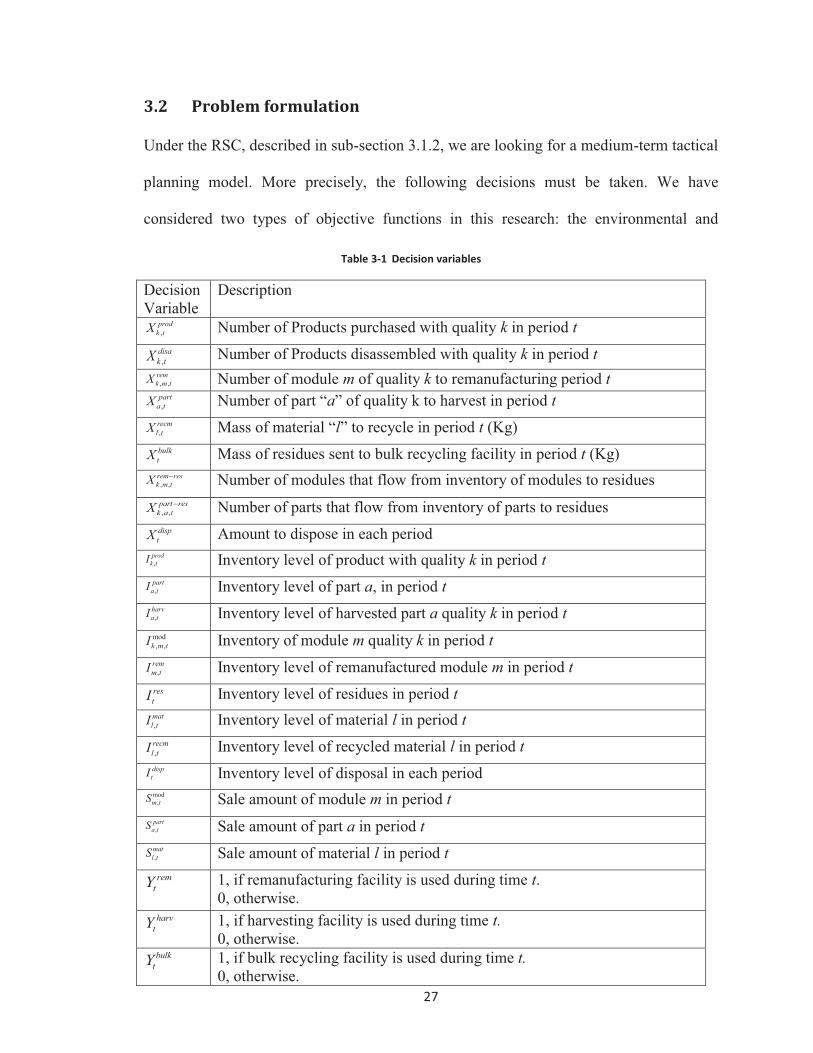
3.2 Problem formulation
Under the RSC, described in sub-section 3.1.2, we are looking for a medium-term tactical
planning model. More precisely, the following decisions must be taken. We have
considered two types of objective functions in this research: the environmental and
Decision Variable
Description
,prod
k tX Number of Products purchased with quality k in period t
,disak tX Number of Products disassembled with quality k in period t
, ,remk m tX Number of module m of quality k to remanufacturing period t
,part
a tX Number of part “a” of quality k to harvest in period t
,recml tX Mass of material “l” to recycle in period t (Kg)
bulktX Mass of residues sent to bulk recycling facility in period t (Kg)
, ,rem resk m tX � Number of modules that flow from inventory of modules to residues
, ,part res
k a tX � Number of parts that flow from inventory of parts to residues disptX Amount to dispose in each period
,prod
k tI Inventory level of product with quality k in period t
,part
a tI Inventory level of part a, in period t
,harva tI Inventory level of harvested part a quality k in period t mod, ,k m tI Inventory of module m quality k in period t
,remm tI Inventory level of remanufactured module m in period t restI Inventory level of residues in period t
,matl tI Inventory level of material l in period t
,recml tI Inventory level of recycled material l in period t disptI Inventory level of disposal in each period mod
,m tS Sale amount of module m in period t
,part
a tS Sale amount of part a in period t
,matl tS Sale amount of material l in period t
remtY 1, if remanufacturing facility is used during time t.
0, otherwise. harv
tY 1, if harvesting facility is used during time t. 0, otherwise.
bulktY 1, if bulk recycling facility is used during time t.
0, otherwise.
Table 3-1 Decision variables
Page 37
28
financial ones. Regarding the environmental concerns, we aim to maximize the total
quantity of the EOL product acquisition. On the other hand, the financial objective
function seeks to maximize the profit. Since these two objective functions are conflicting,
improvement in one of them requires degradation in the other. Therefore we apply the
epsilon constraint method to find the pareto-front solutions and the trade-off between the
two objective functions. The epsilon-constraint method is explained in sub-section 3.3.
The following assumptions are considered in formulating the problem.
� One type of product is considered.
� No back order cost is considered in the model.
� Products of good quality yield good quality modules with less remanufacturing
cost.
� Products of poor quality yield poor quality modules with more remanufacturing
cost.
� Different quality levels of modules are brought up to one standard quality level
after remanufacturing.
� A set-up cost is considered in order to use a facility in each period.
� Each facility consists of a number of machines and workers to process different
tasks. The capacity of machines and labors is assumed to be limited.
� Demand is forecasted for the entire time period in a deterministic manner and
each time period could be a month.
The mathematical model is explained in the following.
Page 38
29
3.2.1 Mathematical model
In this section, we propose an integrated acquisition and recovery production planning
model under the context of durable products reverse supply chain. The model integrates
the acquisition, disassembly, production, sales and inventory planning decisions. We
formulate this multi-period tactical planning problem as a mixed integer linear
programming model as follows:
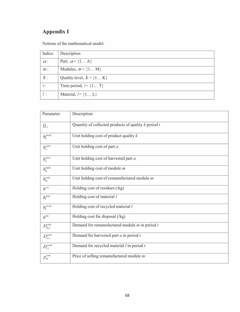
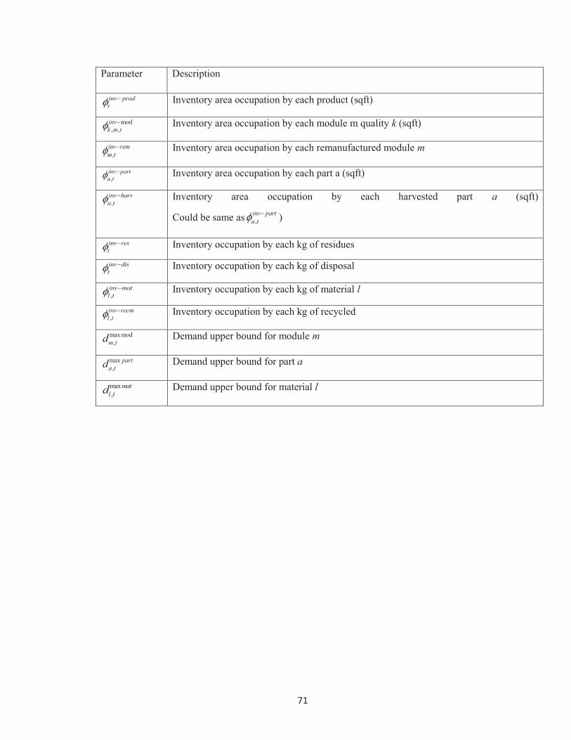
The notions are described in appendix I.
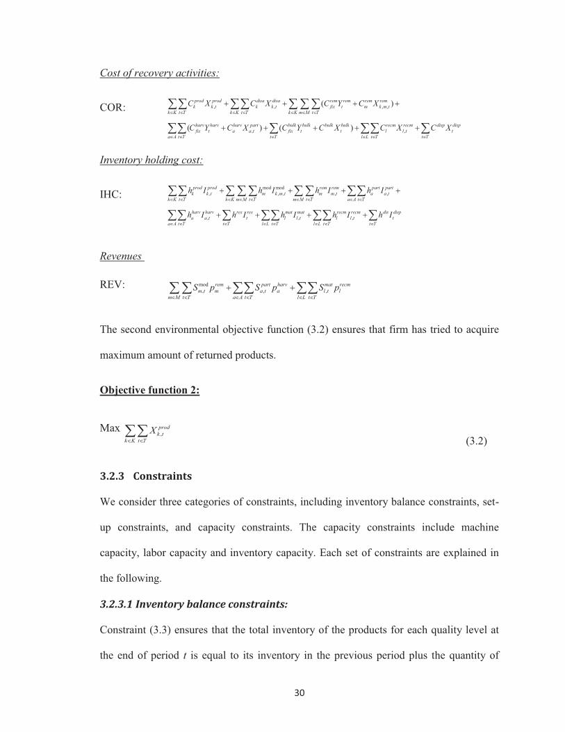
3.2.2 Objective functions
The first financial objective function (3.1) aims at maximizing the total revenue minus
the cost of recovery and inventory over the planning horizon. Total revenue is calculated
as the income obtained from selling the remanufactured modules, harvested parts and
recycled materials.
Objective Function 1:
Max Profit = REV-COR-IHC (3.1)
Revenue (REV) is the income obtained by selling the recovered entities to the market.
Cost of recovery activities (COR) consist of the cost of buying used products from both
quality levels, disassembly process, remanufacturing as well as set-up fixed costs for
remanufacturing in each period, harvesting and refurbishing costs which are mostly labor
intensive, besides harvesting set-up cost, material and bulk recycling processing cost. It
also includes the cost associated with the disposal of useless residues. Inventory costs
(IHC) include the overall cost of keeping the products, modules (before and after
remanufacturing), parts (before and after harvesting), materials (before and after
recycling), residues and disposal over the entire planning periods.
Page 39
30
Cost of recovery activities:
COR: , , , ,
, ,
( )
( ) ( )
prod prod disa disa rem rem rem remk k t k k t fix t m k m t
k K t T k K t T k K m M t T
harv harv harv part bulk bulk bulk bulk recm recm disp dispfix t a a t fix t t l l t t
a A t T t T l L t T t T
C X C X C Y C X
C Y C X C Y C X C X C X
� � � � � � �
� � � � � �
� � � �
� � � � �
�� �� ���
�� � �� �
Inventory holding cost:
IHC: mod mod
, , , , ,
, , ,
prod prod rem rem part partk k t m k m t m m t a a t
k K t T k K m M t T m M t T a A t T
harv harv res res mat mat recm recm dis dispa a t t l l t l l t t
a A t T t T l L t T l L t T t T
h I h I h I h I
h I h I h I h I h I
� � � � � � � � �
� � � � � � � �
� � � �
� � � �
�� � �� �� ��
�� � �� �� �
Revenues
REV: mod, , ,
rem part harv mat recmm t m a t a l t l
m M t T a A t T l L t TS p S p S p
� � � � � �
� ��� �� ��
The second environmental objective function (3.2) ensures that firm has tried to acquire
maximum amount of returned products.
Objective function 2:
Max ,
prodk t
k K t TX
� ���
(3.2)
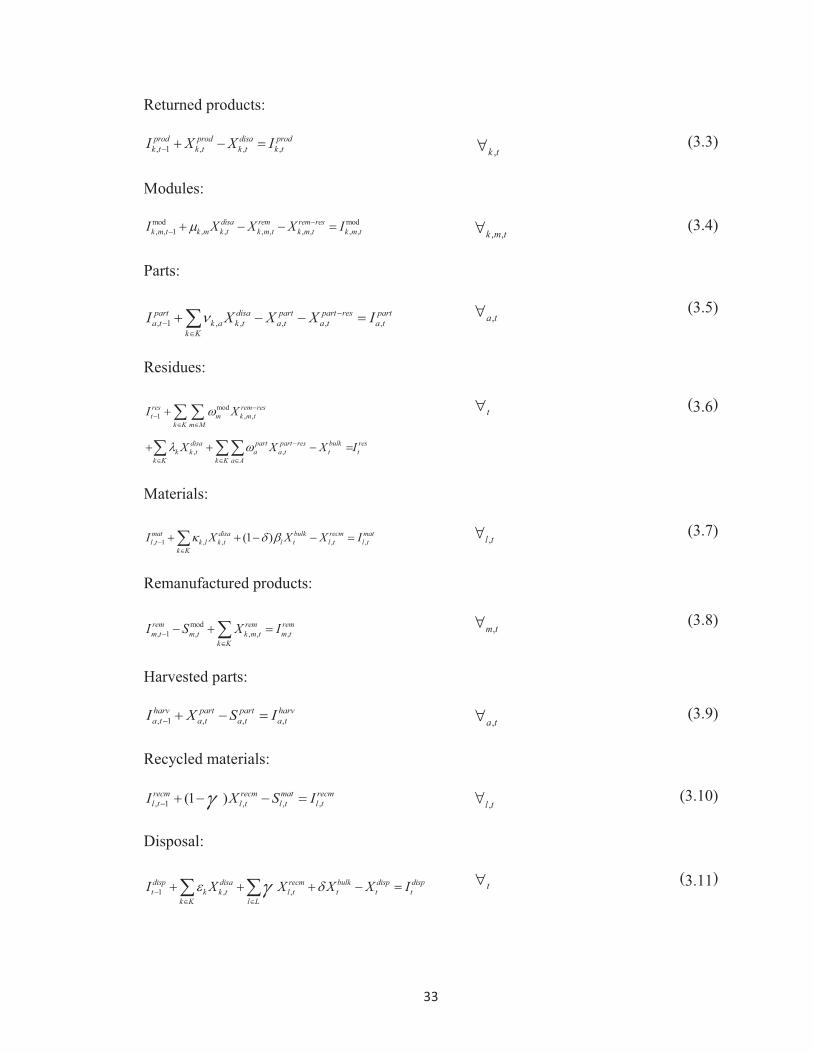
3.2.3 Constraints
We consider three categories of constraints, including inventory balance constraints, set-
up constraints, and capacity constraints. The capacity constraints include machine
capacity, labor capacity and inventory capacity. Each set of constraints are explained in
the following.
3.2.3.1 Inventory balance constraints:
Constraint (3.3) ensures that the total inventory of the products for each quality level at
the end of period t is equal to its inventory in the previous period plus the quantity of
Page 40
31
products of the same quality level acquired ( ,prod
k tX ) at the beginning of that period minus
the quantity of products that are sent to disassembly ( ,disak tX ), in that period. Constraint
(3.4) ensures that the total inventory for each module of quality k at the end of period t is
equal to its inventory in the previous period plus the quantity of the modules of the same
quality extracted after disassembly, minus the amount of modules shipped from the
inventory to the remanufacturing facility ( , ,remk m tX ) and the bulk recycling ( , ,
rem resk m tX � )
facility in that period. In this constraint, ,k m� is the number of module type m available in
each product quality k. Hence, by multiplying this number by the number of product
disassembled in each period ( ,disak tX ), we calculate the total number of extracted modules.
Constraint (3.5) requires that the total inventory for each part at the end of period t is
equal to its inventory in the previous period plus the quantity of all the same type parts
yielded after disassembly, minus the number of parts shipped out to refurbishing facility
( ,part
a tX ) and residues inventory ( ,part res
a tX � ) in that period. In this constraint, , ,a k t� is the
number of part type a available in each product quality k. By multiplying this number by
,disak tX which is the number of products disassembled the total number of parts yielded
after disassembly is calculated. Constraint (3.6) sets the amount of residues in the
inventory at the end of period t equal to the amount of residues carried over from
previous period plus the amount of residues produced after disassembly, as well as
amounts of modules and parts coming from modules and parts inventories, minus the
amount of residues sent to bulk recycling in that period ( bulktX ). In this constraint, k is
the mass of residues in each product of quality k in kg. modm and part
a are weights of
each module m and part a, respectively. Constraint (3.7) ensures that the total inventory
Page 41
32
for each material at the end of period t is equal to its inventory in the previous period plus
the amount of the same material extracted from disassembly and bulk recycling in that
period minus the amount sent to material recycling ( ,recml tX ). In this constraint, ,k l� is the
mass of material l remained after disassembly of product quality k in kg and l� is the
percentage of bulk recycled residues in material l. Constraint (3.8) requires that the
inventory of remanufactured modules at the end of period t is equal to its inventory from
previous period plus the amount of remanufactured modules added to the inventory in the
same period minus the quantity sold in that period. Constraint (3.9) sets the inventory of
harvested parts at the end of period t equal to its inventory from previous period plus the
amount of harvested parts at the harvesting facility in the same period minus the sale
amount. Constraint (3.10) ensures the inventory of recycled materials at the end of period
t is equal to its inventory from previous period plus a fraction of recycled material at the
manual recycling facility minus the amount sold to the market in that period. In this
constraint, the fraction of recycled material sent to inventory is calculated by multiplying
(1- ) by the total amount of material type l recycled, whereas is the percentage of
recycled material sent to disposal. Constraint (3.11) balances the inventory of disposal in
each period. Disposal inventory in each period is equal to the inventory carried over from
previous period plus the disposal generated from different processes such as disassembly,
material ( ) and bulk recycling, minus the amount which is disposed from stock in that
period. In this constraint, k� is the mass of disassembled product of quality k sent to
disposal in kg, and � is the percentage of recycled residues sent to disposal. Constraints
(3.12) - (3.14) require that the sale amount in each period does not exceed the demand in
that period.
Page 42
33
Returned products:
, 1 , , ,prod prod disa prod
k t k t k t k tI X X I� � � � ,k t� (3.3)
Modules:
mod mod, , 1 , , , , , , , ,
disa rem rem resk m t k m k t k m t k m t k m tI X X X I� �
� � � � �
, ,k m t� (3.4)
Parts:
, 1 , , , , ,part disa part part res part
a t k a k t a t a t a tk K
I X X X I� ��
�
� � � �� ,a t� (3.5)
Residues:
mod1 , ,
, ,
res rem rest m k m t
k K m M
disa part part res bulk resk k t a a t t t
k K k K a A
I X
X X X I
��
� �
�
� � �
�
� � � �
� �
� ��
t� (3.6)
Materials:
, 1 , , , ,(1 )mat disa bulk recm matl t k l k t l t l t l t
k KI X X X I� � ��
�
� � � � �� ,l t� (3.7)
Remanufactured products:
mod, 1 , , , ,
rem rem remm t m t k m t m t
k KI S X I�
�
� � �� ,m t� (3.8)
Harvested parts:
, 1 , , ,harv part part harva t a t a t a tI X S I� � � � ,a t� (3.9)
Recycled materials:
, 1 , , ,(1 )recm recm mat recml t l t l t l tI X S I � � � � � ,l t� (3.10)
Disposal:
1 , ,disp disa recm bulk disp dispt k k t l t t t t
k K l LI X X X X I� � �
� �
� � � � �� � t� (3.11)
Page 43
34
mod max mod, ,m t m tS d�
,m t� (3.12)
max, ,
part parta t a tS d�
,a t� (3.13)
max, ,mat matl t l tS d�
,l t� (3.14)
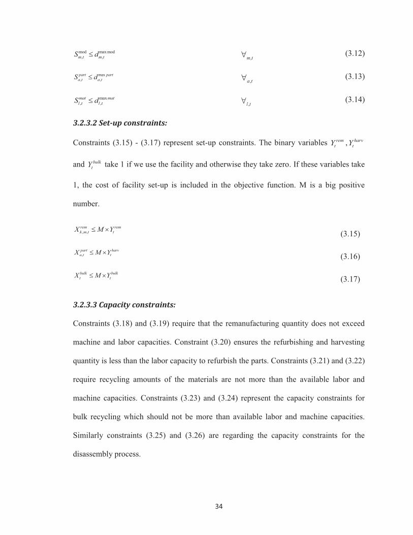
3.2.3.2 Set-up constraints:
Constraints (3.15) - (3.17) represent set-up constraints. The binary variables remtY , harv
tY
and bulktY take 1 if we use the facility and otherwise they take zero. If these variables take
1, the cost of facility set-up is included in the objective function. M is a big positive
number.
, ,rem remk m t tX M Y� � (3.15)
,part harv
a t tX M Y� � (3.16)
bulk bulkt tX M Y� � (3.17)
3.2.3.3 Capacity constraints:
Constraints (3.18) and (3.19) require that the remanufacturing quantity does not exceed
machine and labor capacities. Constraint (3.20) ensures the refurbishing and harvesting
quantity is less than the labor capacity to refurbish the parts. Constraints (3.21) and (3.22)
require recycling amounts of the materials are not more than the available labor and
machine capacities. Constraints (3.23) and (3.24) represent the capacity constraints for
bulk recycling which should not be more than available labor and machine capacities.
Similarly constraints (3.25) and (3.26) are regarding the capacity constraints for the
disassembly process.
Page 44
35
Labor/machine capacity:
, , ,rem lab rem lab remk m t m t t
k K m MX W� � �
� �
�� � t� (3.18)
, , ,rem mach rem mach remk m t m t t
k K m MX W� � �
� �
�� � t� (3.19)
, ,part lab part lab part
a t a t ta A
X W� � �
�
�� t� (3.20)
, ,recm lab recm lab recml t l t t
l LX W� � �
�
�� t� (3.21)
, ,recm mach recm mach recml t l t t
l LX W� � �
�
�� t� (3.22)
bulk lab bulk lab bulkt t tX W� � ��
t� (3.23)
bulk mach bulk mach bulkt t tX W� � �� t� (3.24)
, ,disa lab disa lab disak t k t t
k KX W� � �
�
�� t� (3.25)
, ,disa mach disa machin disak t k t t
k KX W� � �
�
�� t� (3.26)
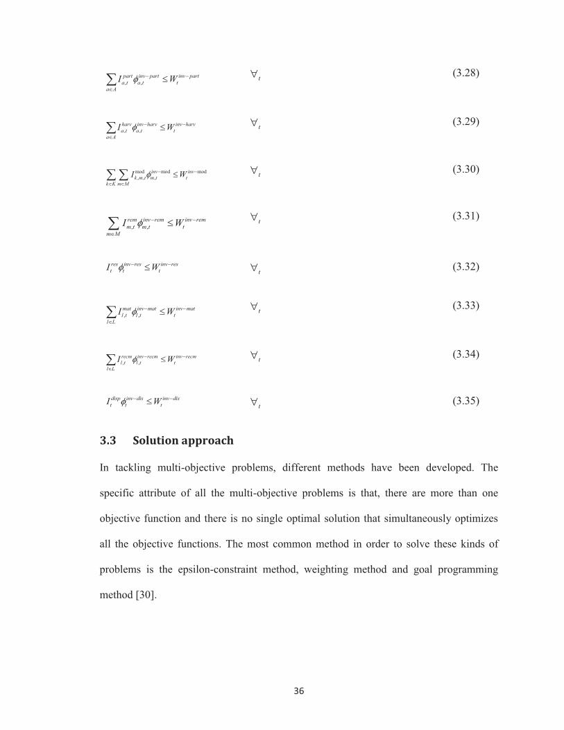
Constraint (3.27) ensures that the inventory of products for both quality levels does not
exceed the total available space of the stock in each period. In a very similar way
constraints (3.28) - (3.35) require that the inventory of disassembled parts, harvested
parts, modules, remanufactured modules, residues, material, recycled materials and
disposal does not exceed their total available inventory capacity.
Inventory capacity:
, ,prod inv prod inv prod
k t k t tk K
I W� � �
�
�� t� (3.27)
Page 45
36
, ,part inv part inv part
a t a t ta A
I W� � �
�
�� t� (3.28)
, ,harv inv harv inv harva t a t t
a AI W� � �
�
�� t� (3.29)
mod mod mod, , ,
inv invk m t m t t
k K m MI W� � �
� �
�� � t� (3.30)
, ,rem inv rem inv remm t m t t
m MI W� � �
�
�� t� (3.31)
res inv res inv rest t tI W� � ��
t� (3.32)
, ,mat inv mat inv matl t l t t
l LI W� � �
�
�� t� (3.33)
, ,recm inv recm inv recml t l t t
l LI W� � �
�
�� t� (3.34)
disp inv dis inv dist t tI W� � ��
t� (3.35)
3.3 Solution approach
In tackling multi-objective problems, different methods have been developed. The
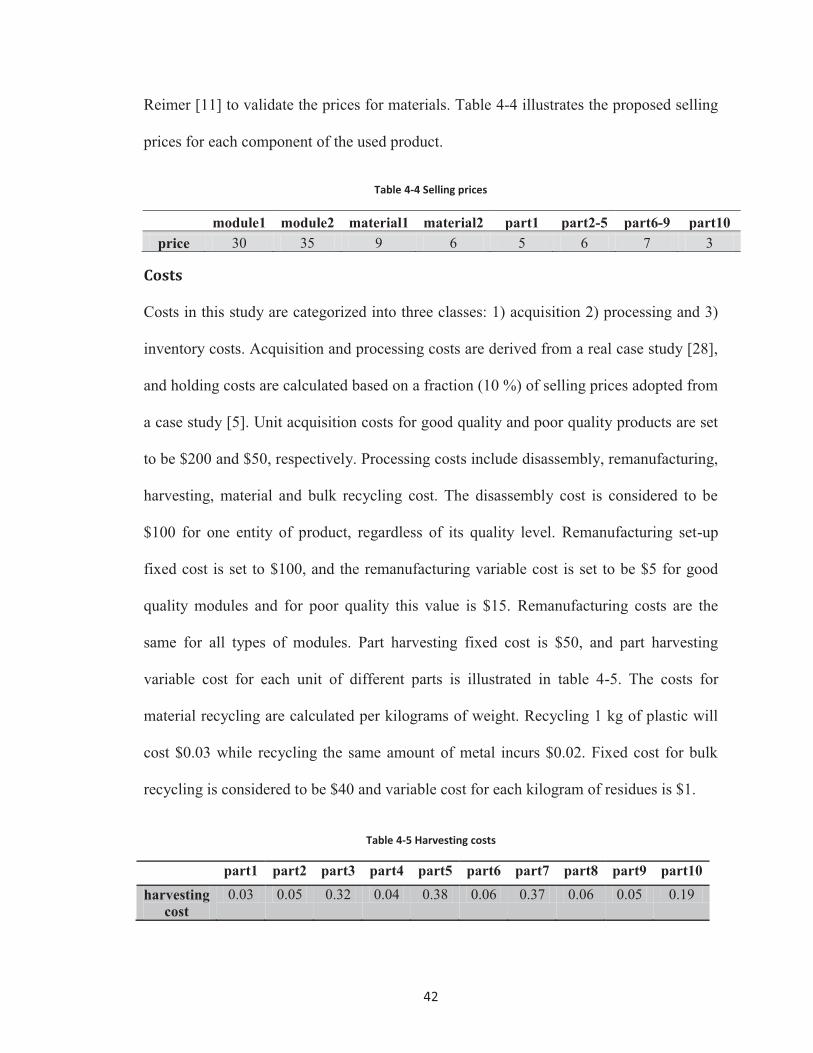
specific attribute of all the multi-objective problems is that, there are more than one
objective function and there is no single optimal solution that simultaneously optimizes
all the objective functions. The most common method in order to solve these kinds of
problems is the epsilon-constraint method, weighting method and goal programming
method [30].
Page 46
37
In the weighting method, different weights are assigned to each objective function. Then
theses objective functions are combined and transferred to one objective function to
produce a set of non-dominated solutions.
Goal programming is an effective method to find a definite solution rather than a set of
non-dominated solutions. In this method a goal value is set for each objective function
and the deviations from the goal value are minimized.
In this research, we applied the epsilon constraint method in order to solve the bi-
objective model. In this method, one objective function is optimized while the other
objective functions are considered as constraints. These constraints are bounded with
some values, and by varying these bounds, a set of “most-preferred” solutions are
obtained. The most preferred solutions are the ones that improve at least one of the
objective functions; these are also called pareto-optimal, non-dominated and non-inferior
solutions. On the other hand, the solutions that do not improve any of the objective
functions and are dominated by better solutions would be eliminated [32-33]. To gain a
better insight into this method, this method is explained in details for a bi-objective
optimization problem, as follows:
First, the optimization model for each objective function is solved individually, 1X and
2X are the optimal solutions corresponding to the each objective. * 11 ( )Z X and 1
2 ( )Z X
are the objective function values associated with solution 1X . Similarly, the objective
function value for 2X are 21( )Z X and * 2
2 ( )Z X .
Second, a pay-off table is constructed as it is shown in table 3-2. The pay-off table values
are calculated as follows. In this method, one objective function is chosen as primary
objective function, the second objective is transferred into the constraint of the first
Page 47
38
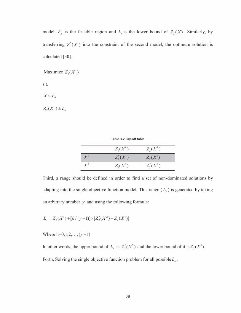
model. dF is the feasible region and nL is the lower bound of 2 ( )Z X . Similarly, by
transferring * 11 ( )Z X into the constraint of the second model, the optimum solution is
calculated [30].
Maximize 1( )Z X
s.t.
dX F�
2 ( ) nZ X L�
Table 3-2 Pay-off table
1( )kZ X 2 ( )kZ X
1X * 11 ( )Z X 1
2 ( )Z X
2X 21( )Z X * 2
2 ( )Z X
Third, a range should be defined in order to find a set of non-dominated solutions by
adapting into the single objective function model. This range ( nL ) is generated by taking
an arbitrary number and using the following formula:
1 * 2 12 2 2( ) [ / ( 1)] [ ( ) ( )]nL Z X h Z X Z X � � � � �
Where h=0,1,2,…, ( 1) �
In other words, the upper bound of nL is * 22 ( )Z X and the lower bound of it is 1
2 ( )Z X .
Forth, Solving the single objective function problem for all possible nL .
Page 48
39
Chapter 4 Case study and computational experiment
In this chapter we first provide the details of our case study, and then we present the
numerical results of applying the proposed model and solution methodology on the case
study. A sensitivity analysis is also conducted for both objective functions at the end of
this chapter.
4.1 Case study
It is worth mentioning that finding a case study with representative data was one of the
most important challenges in this study. The reason lies behind the fact that none of the
existing RSC tactical planning models in the literature are formulated based on a
complete bill-of-material similar to the one investigated in this thesis. Consequently,
none of them include all recovery options with their corresponding parameters.
The case study considered in this research is an academic case focused on electronic used
products. The corresponding data are inspired by the real business case data available in
the literature [7, 28, 9, and 6]. Furthermore, they are also validated and tested several
times according to some of the real business data available on internet. In the following,
the problem data are presented.
4.1.2 Problem data
Returns
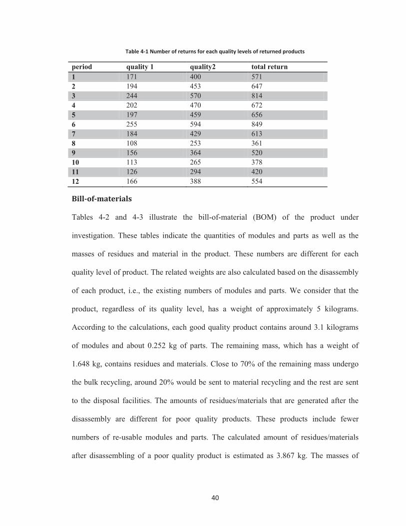
Table 4-1 shows the amount of returns for the used products that are collected at the
collection site at each period. This table is calculated from data based on the real returns
data from the work of Jayaraman [9]. There are two different quality levels of returned
products. Good quality and poor quality. We have considered an estimated value of 30%
of our returns as good quality products, and the rest (70%) belongs to the poor quality.
Page 49
40
Table 4-1 Number of returns for each quality levels of returned products
period quality 1 quality2 total return 1 171 400 571 2 194 453 647 3 244 570 814 4 202 470 672 5 197 459 656 6 255 594 849 7 184 429 613 8 108 253 361 9 156 364 520 10 113 265 378 11 126 294 420 12 166 388 554
Bill-of-materials
Tables 4-2 and 4-3 illustrate the bill-of-material (BOM) of the product under
investigation. These tables indicate the quantities of modules and parts as well as the
masses of residues and material in the product. These numbers are different for each
quality level of product. The related weights are also calculated based on the disassembly
of each product, i.e., the existing numbers of modules and parts. We consider that the
product, regardless of its quality level, has a weight of approximately 5 kilograms.
According to the calculations, each good quality product contains around 3.1 kilograms
of modules and about 0.252 kg of parts. The remaining mass, which has a weight of
1.648 kg, contains residues and materials. Close to 70% of the remaining mass undergo
the bulk recycling, around 20% would be sent to material recycling and the rest are sent
to the disposal facilities. The amounts of residues/materials that are generated after the
disassembly are different for poor quality products. These products include fewer
numbers of re-usable modules and parts. The calculated amount of residues/materials
after disassembling of a poor quality product is estimated as 3.867 kg. The masses of
Page 50
41
residues, materials and disposal corresponding to both qualities are illustrated in table 4-3.
Based on a study provided by Sodhi and Reimer [11], the percentages of recovered
materials in this table are estimated. Hence, in our entire experiment, we set the fractions
of the recovered materials to 30% and 70% for plastic and metal, respectively.
Table 4-2 The number and weights of parts and modules (BOM)
part quantity weight module quantity weight quality1 qulity2 quality1 qulity2
part1 1 1 0.05 module1 1 1 0.25 part2 3 1 0.05 module2 3 1 0.5 part3 2 1 0.05 part4 6 5 0.05 part5 2 1 0.05 part6 4 1 0.05 part7 2 1 0.05 part8 3 2 0.05 part9 2 1 0.05 part10 2 1 0.05
Table 4-3 Mass of residues, materials and disposal after disassembly
Quality Mass of disposal(kg)
Mass sent to material (kg) recycling
Mass sent to bulk
recycling (kg)
metal plastic quality1 0.1648 0.23072 0.09888 1.1536 quality2 0.3867 0.54138 0.23202 2.7069
Prices
The selling prices of the recovered modules and parts are inspired from the work of
Srivastava [28]. We also used different internet sources [29], and the work of Sodhi and
Page 51
42
Reimer [11] to validate the prices for materials. Table 4-4 illustrates the proposed selling
prices for each component of the used product.
Table 4-4 Selling prices
module1 module2 material1 material2 part1 part2-5 part6-9 part10 price 30 35 9 6 5 6 7 3
Costs
Costs in this study are categorized into three classes: 1) acquisition 2) processing and 3)
inventory costs. Acquisition and processing costs are derived from a real case study [28],
and holding costs are calculated based on a fraction (10 %) of selling prices adopted from
a case study [5]. Unit acquisition costs for good quality and poor quality products are set
to be $200 and $50, respectively. Processing costs include disassembly, remanufacturing,
harvesting, material and bulk recycling cost. The disassembly cost is considered to be
$100 for one entity of product, regardless of its quality level. Remanufacturing set-up
fixed cost is set to $100, and the remanufacturing variable cost is set to be $5 for good
quality modules and for poor quality this value is $15. Remanufacturing costs are the
same for all types of modules. Part harvesting fixed cost is $50, and part harvesting
variable cost for each unit of different parts is illustrated in table 4-5. The costs for
material recycling are calculated per kilograms of weight. Recycling 1 kg of plastic will
cost $0.03 while recycling the same amount of metal incurs $0.02. Fixed cost for bulk
recycling is considered to be $40 and variable cost for each kilogram of residues is $1.
Table 4-5 Harvesting costs
part1 part2 part3 part4 part5 part6 part7 part8 part9 part10 harvesting
cost 0.03 0.05 0.32 0.04 0.38 0.06 0.37 0.06 0.05 0.19
Page 52
43
Table 4-6 indicates the inventory costs for each unit of different parts, modules, material
and products. These costs are defined based on the quality and size of each module/part.
The Initial inventory for each part is considered to be zero. Holding costs are assumed to
be the same for remanufactured modules, harvested parts and recycled materials with
modules, parts and materials before being processed.
Table 4-6 Inventory costs
module1 module2 material1 material2 Product quality1
Product quality2
holding cost 3 3.5 0.9 0.6 20 5
part1 part2 part3-5 part6-9 part10
holding cost 0.5 0.6 0.6 0.7 0.3
Demand
In order to find the demand for each module/part, we multiplied the number of product
demand by the number of modules/parts that exist in that product, based on the BMO of
this product. We assume the demand for a (hypothetical) electronic product (e.g., PC) in
each period has a uniform distribution ranging between 250-500 units. According to
tables 4-2 and 4-3, the demand for each module and part is calculated. In order to find the
demand for each material in each period, a fraction of a product’s weight is considered.
This fraction is 40% and 30% for metal and plastic.
Capacity consumptions are considered not to be the same for different modules. Capacity
consumption for poor quality modules are twice as the capacity consumption of good
quality modules for both machine and labor. This quantity is 2 units for poor quality
modules and 1 unit for good quality modules. Labor and machine part harvesting capacity
is assumed to be the same for all the parts and it is set to 1. Labor, machine and inventory
Page 53
44
consumption for each kg of materials are considered to be 1. We consider a large storage
capacity for the inventory of modules, parts and residues (i.e., 10000, 10000 and 20000,
respectively).
4.2 Numerical results
4.2.1 Experimental details
Experiments were conducted using computer 2.8 GHz Pentium® Dual-Core Opteron 64-
bit processors and 4 GB RAM. The bi-objective mixed integer Linear Programming
model is coded and solved with CPLEX OPL version 12.3, 32 bit and we have
implemented the sensitivity analysis by the aid of Minitab16.2.3. The bi-objective
problem includes 576 inventory balance constraints, 216 capacity constraints and 984
decision variables.
4.2.2 Epsilon-constraint method results
As explained in section 3.3 of this thesis, the epsilon-constraint method is used to solve
the bi-objective tactical planning models. In this sub-section we provide the results of the
application of the epsilon-constraint method in our case study. For this purpose a payoff
table is calculated, as it can be seen in table 4-7.
Table 4-7 Payoff table for two objectives
1( )kZ X 2 ( )kZ X
1X * 11 ( )Z X =247,809 1
2 ( )Z X =5,723
2X 21( )Z X =188,972 * 2
2 ( )Z X =7,055
The payoff table is calculated by finding the individual optimum of each objective
function. Further, by adding the other objective function as a constraint to the primary
objective function we find the upper and lower bounds for the second objective function.
Page 54
45
In table 4-7, 12 ( )Z X =5723 and * 2
2 ( )Z X =7055 are the lower and upper bounds of the
second objective function, respectively. By picking 20 as the value for and using the
following equation, we divided the range of the second objective to 20 equivalent
intervals.
1 * 2 12 1 2 2( ) [ / ( 1)] [ ( ) ( )]nL Z X h Z X Z X � � � � �
By plugging different values of each nL as the lower bound of the corresponding
constraint (i.e., second objective function) into the bi-objective model, we generated 20
non-dominated solutions. Table 4-8 illustrates the range of both objective function values
over the range of non-dominated solutions. It can be observed that while moving from
one pareto solution to the other, one objective is improved and the other is degraded. The
last two columns in table 4-8, represent the deviation (%) from the optimal objective
value for each non-dominated solution.
Page 55
46
Table 4-8 Payoff table for gamma=20
Z2 Z1 Z2 % Z1%
7055 188972 100 76.25712
6985 194882 99.0063 78.64202
6915 200010 98.01261 80.71135
6845 205052 97.01891 82.74599
6775 209847 96.02522 84.68094
6704 214408 95.03152 86.52147
6634 218517 94.03782 88.17961
6564 222401 93.04413 89.74694
6494 226070 92.05043 91.22752
6424 229418 91.05673 92.57856
6354 232798 90.06304 93.94251
6284 236178 89.06934 95.30647
6214 239131 88.07565 96.49811
6144 241462 87.08195 97.43875
6074 243573 86.08825 98.29062
6003 245486 85.09456 99.06258
5933 246804 84.10086 99.59445
5863 247508 83.10717 99.87854
5793 247809 82.11347 100
5723 247809 81.11977 100
4.2.3 Analysis of the results
The decision maker has to choose the best compromise solution among the set of pareto-
optimal non-dominated solutions. In order to facilitate the process of decision making, we
have shown the results in terms of the percentage of deviation from optimal objective
value for each objective function in figure 4-1. This figure illustrates the relationship
between the two competing objective functions. The top left point represent the optimum
Page 56
47
acquisition quantity (second objective) and the bottom right point indicates the optimum
profit (first objective).
Generally, good quality returned products are all purchased due to their low recovery cost,
more recoverable modules and high profitability. High quality returned products are also
scarce and limited, comparing to the poor quality products. Hence, the maximization of
our environmental objective function would target the acquisition of poor quality
products. With the same reasoning, it would be able to prevent the high penalties that the
producer is charged by legislation due to landfilling of the EOL products. Based on the
experimental results, it can be concluded that if the decision maker aims for maximum
profit, he is lacking 18% of maximum acquisition which mainly include poor quality
products. Furthermore, by increasing the acquisition quantity to 8%, the firm’s profit
would be decreased by 6% from its optimal value. Therefore, it is crucial to utilize the
tradeoffs between both objectives prior to make decisions on acquisition amounts of
returned products. Due to the fact that firms are required to participate in environmentally
friendly activities, acquiring more amounts of used product not only decreases the landfill
amounts of EOL’s, but also prevents the firm from paying high penalties to governments.
By using figure 4-1, the manager would be able to choose the best solution according to
the profit and acquisition amounts that the firm is willing to obtain.
Page 57
48
Figure 4-1 Trade-off graph for two objective functions
4.3 Sensitivity analysis
In order to determine how different model parameters affect each objective function, a set
of sensitivity analysis tests are conducted. In the present work, we are interested into
studying the simultaneous influence of several parameters on the both objective functions.
Therefore, we have used the full factorial design for this purpose.
Factorial design
Factorial experiments involve the analysis of two or more factors on a response variable.
A full factorial design allows for studying of the effect of each factor and their interaction
on the response variable [20].
80
82
84
86
88
90
92
94
96
98
100
76 78 80 82 84 86 88 90 92 94 96 98 100
Opt
imum
acq
uisi
tion
quan
tity
%
Optimum profit %
Z2 % Z1%
Linear (Z2 % Z1%)
Page 58
49
The sensitivity analysis, on both models is conducted based on factorial design, where the
factors are fixed at two levels, and two replications for each set of experiments are run.
Inspired by the common practice in the literature and also according to the order of
magnitude of nominal values of different parameters, variations of parameters (factors)
have been considered as +20% and -20% of their nominal values. In total there are
different combinations of factors in the experiment. By considering two replications for
each experiment we ran × 2=128 different experiments. Each replication is generated
based on a random demand that follows a uniform distribution ranging between
[250,500]. Hence, in each replication we generate a new demand profile based on the
uniform distribution.
4.3.1 Sensitivity analysis on the financial objective function- Profit
maximization
In this experiment, we study six different factors, such as total demand, quantity of
returns, price, acquisition costs, holding costs and the ratio of good to poor quality return.
We are interested to investigate the influence of mentioned factors on the two key
performance indicators (KPIs). These KPIs are profit and total acquisition amount.
4.3.1.1 Factors effect on profit (KPI 1)
According to figure 4-2 and table 4-9 (ANOVA table), following conclusions are made:
Page 59
50
4003002001000-100
99.9
99
9590
80706050403020
10
5
1
0.1
Standardized Effect
Perc
ent
A DemandB Q uantity of ReturnsC PriceD A cquisition C ostE Holding costF Good Q uality /Poor Q uality
Factor Name
Not SignificantSignificant
Effect Type
BCEF
BCDFCDF
BDF
BCF
BCE
BCD
ACF
ABFACEABC
DF
CF
CE
CD
BF
BE
BD
BC
AEACABF
E
D
CB
A
Normal Plot of the Standardized Effects(response is Total Profit, Alpha = 0.05)
Figure 4-2 Normal plot of the effect on Total profit
Table 4-9 ANOVA table for profit
Term Effect Coef SE Coef T P Constant 291,951 635.7 459.26 0.000
Demand 23,054 11527 635.7 18.13 0.000
Quantity of returns
79,756 39878 635.7 62.73 0.000
Price 475,795 237897 635.7 374.23 0.000 Acquisition Cost
-142,090 -71045 635.7 -111.76 0.000
Holding cost
-5,181 -2591 635.7 -4.08 0.000
Good quality/ Poor quality
21,445 10723 635.7 16.87 0.000
� The most influential factors affecting the profit are selling price of recovered
items, quantity of returns and the acquisition cost.
Page 60
51
� Price and quantity of returns have a positive effect while acquisition cost has a
negative influence on the profit.
+1-1
600000
450000
300000
150000
0+1-1 +1-1
+1-1
600000
450000
300000
150000
0+1-1 +1-1
Demand
Mea
n
Quantity of Returns Price
Acquisition Cost Holding cost Good Quality/Poor Quality
Main Effects Plot for Total ProfitData Means
Figure 4-3 Main effect plot for total profit
According to the main effects plot for total profit (figure 4-3), it is worth to discuss the
effects of price, quantity of returns and acquisition costs more thoroughly.
Based on figure 4-3 and table 4-9, it can be concluded that by increasing the selling
prices of recovered items, profit would be increased significantly, this is due to the fact
that increase in price lead to the revenue increase while the costs remain the same.
Figure 4-3 also indicates that by increasing the quantity of returns, profit is increased.
However, this effect is relatively small comparing to the effects of changes in the selling
price.
Unlike selling price and quantity of returns, acquisition cost has a negative impact on the
profit. By increasing the acquisition price, the profit would be decreased and vice versa.
Page 61
52
+1-1 +1-1 +1-1 +1-1 +1-1
500000
250000
0
500000
250000
0
500000
250000
0
500000
250000
0
500000
250000
0
Demand
Quantity of Returns
Price
Acquisition Cost
Holding cost
Good Quality/Poor Quality
-1+1
Demand
-1+1
of ReturnsQuantity
-1+1
Price
-1+1
CostAcquisition
-1+1
costHolding
Interaction Plot for Total ProfitData Means
Figure 4-4 Interactions plot for total profit
An interesting finding from the interaction plot in figure 4-4, shows that some factors
such as price and holding cost or price and ratio of good to poor quality returns are totally
independent. Parallel graphs prove that changes in one factor could not affect the
objective function resulted by other factor. In contrary, some factors such as return
quantity and price happen to have an interaction. More precisely, when the price is low,
changes in the quantity of returns do not affect the profit. But when the price is increased,
profit will increase for more amounts of returns.
According to the same plot in figure 4-4, it can be concluded that the quantity of returns
has no interaction with other factors in affecting the profit except for the ratio of qualities.
In other words, for low level of returns, changes in the ratio of good to poor quality of
returns do not affect the profit. Whereas for larger amounts of returns the profit would be
Page 62
53
increased significantly by increasing the ratio of good to poor quality. Moreover, when
the price is low, changes in the ratio of good quality to poor quality would not affect the
total acquisition of poor quality returns but for a higher price it may decrease the poor
quality return acquisition to some extent.
4.3.1.2 Factors Effect on total acquisition amount (KPI2)
According to the normal plot for total acquisition which is shown in figure 4-5 and the
ANOVA table 4-10, important factors affecting the total acquisition incorporate price and
quantity of returns positively and acquisition cost and ratio of good to poor quality
returns negatively.
As it is shown in figure 4-6 and 4-7, increasing the price of recovered items would
increase the acquisition amounts of both poor and good quality. The reason is that by
acquiring more returned items higher revenue is expected due to higher prices of
recovered items.
By analyzing the main effect plots in figures 4-6 and 4-7, it can be observed that by
increasing the quantity of products return, the acquisition quantity of good quality
products is increased while the acquisition of poor qualities does not change. An
important key point could be concluded that by increasing the quantity of returns, the
model tends to acquire more of good quality rather than poor quality. This is based on the
fact that recovering good quality products are more profitable. In other words, the model
does not tend to acquire poor quality ones because of their high processing cost and low
value.
Another finding from the normal plot (figure 4-5) and table 4-10 is that by increasing the
ratio of good to poor quality, total acquisition would be decreased. This is due to the fact
Page 63
54
that by increasing the ratio of qualities while the total amount is fixed, there would be
more amounts of good quality which produce more recovered items and fewer amounts
of poor quality products which are more costly. Therefore, the model does not need to
acquire high amounts of returns when the ratio of good to poor quality is high.
Another observation regarding total acquisition, is that increasing the acquisition cost,
remarkably decrease the good quality acquisition amount but it does not change the
acquisition of poor quality ones significantly. It could be interpreted based on the
considerable difference between the acquisition price of good and poor qualities.
200150100500-50
99.9
99
9590
80706050403020
10
5
1
0.1
Standardized Effect
Perc
ent
A DemandB Q uantity of ReturnsC PriceD A cquisition C ostE Holding costF Good Q uality /Poor Q uality
Factor Name
Not SignificantSignificant
Effect Type
ABCDFACDF
ABCF
CDF
BCFBCD
ACFABF
ACE
ABC
DF
CF
CE
CD
BF
BD
BC
AF
ACAB
F
E
D
C
BA
Normal Plot of the Standardized Effects(response is Total Acquisition, Alpha = 0.05)
Figure 4-5 Normal plot for total acquisition
Page 64
55
Table 4-10 ANOVA table for total acquisition
Term Effect Coef SE Coef T P Constant 3162.5 10.55 299.75 0.000
Demand 342.9 171.4 10.55 16.25 0.000
Quantity of returns
768.7 384.4 10.55 36.43 0.000
Price 3,560.7 1780.1 10.55 168.71 0.000 Acquisition Cost
-1015.6 -507.8
10.55 -48.13 0.000
Holding cost
-45.9 -23.0 10.55 -2.18 0.033
Good quality/ Poor quality
-836.8 -418.4 10.55 -39.65 0.000
+1-1
2000
1750
1500
1250
1000+1-1 +1-1
+1-1
2000
1750
1500
1250
1000+1-1 +1-1
Demand
Mea
n
Quantity of Returns Price
Acquisition Cost Holding cost Good Quality/Poor Quality
Main Effects Plot for Good Qualiy AcquisitionData Means
Figure 4-6 Main effects plot for good quality acquisition
Page 65
56
+1-1
3000
2000
1000
0+1-1 +1-1
+1-1
3000
2000
1000
0+1-1 +1-1
Demand
Mea
n
Quantity of Returns Price
Acquisition Cost Holding cost Good Quality/Poor Quality
Main Effects Plot for Poor Quality AcquisitionData Means
Figure 4-7 Main effects plot for poor quality acquisition
4.3.2 Sensitivity analysis on the environmental objective function- acquisition
amount maximization
In this set of experiment, we consider total acquisition amount as the only objective
function and we are only interested to investigate the effects of three factors on the total
acquisition. These factors include quantity of returns, demand and ratio of good to poor
quality products.
Page 66
57
1-1
7000
6000
5000
40001-1
1-1
7000
6000
5000
4000
Demand
Mea
n
Quantity of Returns
Good quality/Poor quality
Main Effects Plot for Total AcquisitionData Means
Figure 4-8 Main effects plot for total acquisition
According to the figure 4-8, it can be concluded that only the quantity of returns and the
ratio of good to poor quality returns are affecting the amount of acquisition.
Since total acquisition is the summation of both good and poor quality returns, we are
going to explain the effects of each factor on each quality level separately. Figures 4-9
and 4-10, indicate that by increasing the quantity of returns, the acquisition amount of
both good and poor qualities would be increased. More importantly, by increasing the
ratio of good to poor quality, the model tends to acquire more from the better quality
products. On the other hand, this increase would result in a decrease in the acquisition
amounts of poor quality returns. But according to the main plot effect (figure 4-8), poor
quality returns are more influential by this ratio comparing to the good quality returns.
This fact suggests increasing the ratio of poor over good quality returns will result in a
higher total acquisition amount. While the profit element is excluded in this section, this
Page 67
58
could be explained according to capacity consumptions, inventory and demand
constraints.
1-1
3000
2500
2000
1500
1-1
1-1
3000
2500
2000
1500
Demand
Mea
n
Quantity of Returns
Good quality/Poor quality
Main Effects Plot for Good Quality AcquisitionData Means
Figure 4-9 Main effects plot for good quality acquisition
1-1
5000
4000
3000
2000
10001-1
1-1
5000
4000
3000
2000
1000
Demand
Mea
n
Quantity of Returns
Good quality/Poor quality
Main Effects Plot for Poor Quality AcquisitionData Means
Figure 4-10 Main effects plot for good quality acquisition
Page 68
59
1-1 1-1
8000
6000
4000
8000
6000
4000
Demand
Quantity of Returns
Good quality/Poor quality
-11
Demand
-11
of ReturnsQuantity
Interaction Plot for Total AcquisitionData Means
Figure 4-11 Interaction plot for total acquisition
According to the interaction plot in figure 4-11, it can be concluded that there is no
relation between changes in demand with both quantity of returns and ratio of qualities.
Moreover, there is a relation between quantity of returns and ratio of good to poor quality
in such a way that when the quantity of returns is at its high level, having more poor
quality than good quality products (bigger ratio of poor to good quality) will increase the
acquisition amount.
Page 69
60
Chapter 5 Conclusions and future research
In this chapter, we present a summary of the thesis. We also provide several concluding
remarks based on the problem solution and sensitivity analysis. Future research in this
area is discussed at the end.
5.1 Conclusion
In this research, we developed a bi-objective, multi-period mixed integer linear
programming model for tactical planning in a RSC. We considered two objective
functions, including profit maximization as well as total acquisition amount
maximization. In this problem, the returns are assumed to be durable products which
consist of multiple and various types of components that can be recovered by different
recovery methods. The modular structure of durable products makes them subject to the
all disposition options, such as remanufacturing, harvesting, material and bulk recycling,
and disposal. The proposed model decides on the integrated tactical level decisions such
as acquisition, disassembly and grading, and production planning of different disposition
activities as well as, sales and inventory planning in the reverse supply chain.
The multi-indenture structure of durable products which leads to a complex RSC network
increases the complexity of the proposed model. The model incorporates numerous
decision variables and constraints which are formulated based on a complex bill of
material corresponding to a durable product. In order to validate and test the model, it is
applied on an EOL electronic device. Nevertheless, the model is applicable to similar
RSC networks corresponding to durable products.
Page 70
61
Furthermore, the bi-objective model is solved by the aid of the epsilon-constraint method.
A set of non-dominated solutions are presented for the decision maker and the following
conclusions were obtained:
� The good quality acquisition amount reaches 100% in all the solutions, because of
the profitability of the recovery of good quality products.
� By increasing the acquisition quantity, more poor quality products are acquired,
consequently the recovery cost is increased and profit is decreased.
� The profit reaches its maximum value while the total acquisition takes the lowest
amount among all the possible solutions. Keeping the acquisition at lower
quantities protect the company against high costs of poor quality products
recovery.
� The acquisition amount reaches it maximum by scarifying the profit around 25%
of its optimal value. In return, acquiring poor quality products help the company
to get aligned with the legislations and environmental concerns, particularly,
when the company is obliged to reach a certain amount of EOL recovery.
� By the aid of the non-dominated solutions, the decision maker would be able to
choose the best solution according to the profit and acquisition amounts that the
firm is willing to obtain. The latter also depends on the legislation regarding the
target amount of EOL recovery.
In order to determine how different model parameters affect each objective function and
other KPIs, a set of sensitivity analysis tests are conducted. The following conclusions
are derived for the problem with profit maximization objective:
Page 71
62
� The most influential factors affecting the profit are selling price of recovered
items and quantity of returns positively, and the acquisition cost negatively.
� When the price is low, changes in the quantity of returns do not affect the profit.
But when the price is increased, profit will increase for more amounts of returns.
� For low amounts of returns, changes in the ratio of good to poor quality of returns
do not affect the profit, whereas for large amount of returns the profit would be
increased significantly.
� When the price is low, changes in the ratio of good to poor quality would not
affect the total acquisition of poor quality returns but for a higher price it may
decrease the poor quality return acquisition to some extent.
� Considering the total acquisition amount as the second KPI, we observed that
increasing the price would increase the acquisition amounts of both poor quality
and good quality
� Another key point could be concluded that by increasing the quantity of returns,
the model tends to acquire more of good quality rather than poor quality returns.
This justifies the fact that recovering good quality products are more profitable.
The following conclusions were obtained based on the sensitivity analysis regarding the
environmental objective function (acquisition amount maximization):
� Increasing the ratio of poor over good quality products will result in a higher total
acquisition amount. While the profit element is excluded in this section, this could
be explained according to capacity consumptions, inventory and sales constraints.
Page 72
63
� When the total quantity of returns is at its highest level, having more poor quality
than good quality products (bigger ratio of poor to good quality) results in larger
acquisition amounts, comparing to the low levels of returns quantity.
The key considerations in this study that contribute to the existing literature are as follows:
� An integrated tactical planning model including acquisition, grading and
disposition (remanufacturing, harvesting, recycling and disposal) decisions in the
context of a durable product RSC is proposed.
� A multi-indenture structure is considered for the EOL products. Consequently, all
possible recovery options are taken into account.
� Two objective functions addressing both financial and environmental criteria are
proposed.
� Two quality levels for returns are considered. They differ in the acquisition price,
recovery and processing costs, and the amounts of recoverable components.
5.2 Future research
There are several directions to extend the model presented in this study. Our suggestions
for future research in this area are as follows:
� To consider the uncertainty in the quality of returns. More precisely, considering
the proportions of reusable modules, parts and materials in a returned item of a
given quality level as a random variable instead of a deterministic one, as we did
in the current study.
� To reformulate the problem as a stochastic program or a robust optimization
model while considering the uncertain quality of returns.
Page 73
64
� To integrate the return acquisition pricing problem into the current RSC tactical
planning model. The latter will lead to a non-linear optimization problem.
� To integrate the proposed RSC tactical planning model with the forward supply
chain planning model in the context of a closed-loop supply chain. The idea is to
align the forward and backward flow decisions in such a network.
� To address the RSC tactical planning model in a multi-product setting.
Page 74
65
Refrences
[1] Atasu and Cetinkaya, “Lot Sizing for Optimal Collection and Use of Remanufacturable Returns over a Finite Life-Cycle”, Production and Operations Management, 15(4), 473–487, 2006.
[2] Galbreth and Blackburn,“Optimal Acquisition Quantities in Remanufacturing”, Production and Operations Management,19(1), 61–69, 2009.
[3] Robotis Andreas Robotis, Shantanu Bhattacharya, Luk N. Van Wassenhove, “The effect of remanufacturing on procurement decisions for resellers in secondary markets”, European Journal of Operational Research, 163, 688–705, 2005.
[4] C. Zikopoulos, G. Tagaras, “Production, Manufacturing and Logistics Impact of uncertainty in the quality of returns on the profitability of a single-period refurbishing operation”, European Journal of Operational Research, 182, 205–225, 2007.
[5] M. Denizel, M. Ferguson, and G. Souza, “Multi-period remanufacturing planning with uncertain quality of inputs,”, IEEE Transactions on Engineering Management, 57(3), 394–404, 2010.
[6] M. Ferguson, V. D. Guide Jr, E. Koca, and G. C. Souza, “The value of quality grading in remanufacturing,” Production and Operations Management, 18(3), 300–314, 2009.
[7] Kibum Kim , Iksoo Song, Juyong Kim, BongjuJeong, “ Supply planning model for remanufacturing system in reverse logistics environment”, Computers & Industrial Engineering, 51, 279–287, 2006.
[8] H-H Doh and D-H Lee, “Generic production planning model for remanufacturing systems”, Proceedings of the Institution of Mechanical Engineers, Part B: Journal of Engineering Manufacture, 224(159), 2010.
[9] Vaidyanathan Jayaraman, “Production planning for closed-loop supply Chains with product recovery and reuse”, International Journal of Production Research, 44(5), 981-998, 2006.
[10] J. B. Sheu, Y. H. Chou, and C. C. Hu, “An integrated logistics operational model for green-supply chain management”, Transportation Research Part E: Logistics and Transportation Review, 41(4), 287–313, 2005.
[11] Manbir S. Sodhi and Bryan Reimer, “Models for recycling electronics end-of-life products”, ORSpektrum, 23, 97-115, 2001.
[12] Grit Walther, Thomas Spengler, "Impact of WEEE-directive on reverse logistics in Germany", International Journal of Physical Distribution & Logistics Management, 35(5), 337–361, 2005.
Page 75
66
[13] Ehrgott, M. “Multi-criteria optimization”. Berlin, Springer, 2005.
[14] M. E. Ferguson and G. C. Souza, “Commentary on Closed-loop supply chains”, in Closed-loop supply chains: new developments to improve the sustainability of business practices, 1st ed., M. E. Ferguson and G. C. Souza, Ed. New York: CRC Press, 99-118, 2010.
[15] Chopra, S., & Meindl. Supply chain management: strategy, Planning and operation, Upper saddle River, NJ: Prentice-Hall. 2001.
[16] Guide Jr., V.D.R. and L.N. Van Wassenhove. Managing product returns for remanufacturing, Production and Operations Management, 10(2), 142–155, 2001.
[17] Necati Aras, Tamer Boyaci, and VedatVerter, “Designing the reverse logistic network”, in Closed-loop supply chains: new developments to improve the sustainability of business practices, 1st ed., M. E. Ferguson and G. C. Souza, Ed. New York: CRC Press, 99-118, 2010.
[18] http://www.un-documents.net/unchedec.html, Report of the United Nations Conference on the Human Environment, Stockholm, June 1972.
[19] Guide Jr., V.D.R., R. Teunter, and L.N. Van Wassenhove, “Matching demand and supply to maximize profits from remanufacturing”, Manufacturing & Service Operations Management, 5(4), 303–316, 2003.
[20] Diouglas, C.Montgomery, “Design and Analysis of Experiments”, 2005. Karakayali, I., H. Emir-Farinas, and E. Akcali, “An analysis of decentralized collection and processing of end-of-life products”, Journal of Operations Management, 25(6),1161–1183, 2007.
[21] Bakal, I.S. and E. Akcali, “Effects of random yield in remanufacturing with price-sensitive supply and demand”,. Production and Operations Management, 15(3), 407–420. 2006.
[22] Ray, S., T. Boyaci, and N. Aras, “Optimal prices and trade-in rebates for durable, remanufacturable products”, Manufacturing & Service Operations Management 7(3), 208–228, 2005.
[23] Blackburn, J.D., V.D.R. Guide Jr., G.C. Souza, and L.N. Van Wassenhove, “Reverse supply chains for commercial returns”,. California Management Review, 46(2), 6–22, 2004.
[24] Moritz Fleischmann, Michael R. Galbreth, and George Tagaras, “product acquisition, grading, and disposition tagaras”, in Closed-loop supply chains: new developments to improve the sustainability of business practices, 1st ed., M. E. Ferguson and G. C. Souza, Ed. New York: CRC Press, 99-118, 2010.
Page 76
67
[25] Gilvan C .Souza, “production planning and control for remanufacturing”, in Closed-loop supply chains: new developments to improve the sustainability of business practices, 1st ed., M. E. Ferguson and G. C. Souza, Ed. New York: CRC Press, 99-118, 2010.
[26] Stessel RI, Pelz S, “Air classification of mixed plastics”, In: National Waste Processing Conference Procedings ASME, 333–339, 1994.
[27] Hull JB, Langton CM, Jones AR, “An ultrasonic method for identifying polymeric materials/components for reclamation and recycling”, Macromolecular Reports, 31, 1191–1199, 1994.
[28] Samir K. Srivastava, Rajiv K. Srivastava,"Managing product returns for reverse logistics", International Journal of Physical Distribution & Logistics Management, 36(7), 524 – 546, 2006.
[29] http://www.recycleinme.com. Scrap and recycle market news.
[30] George Mavrotas, “Effective implementation of the e-constraint method in Multi-Objective Mathematical Programming problems”, Applied Mathematics and Computation, 213, 455–465, 2009.
Page 77
68
Appendix I
Notions of the mathematical model.
Indice Description
a : Part, a = {1… A}
m : Modules, m = {1… M}
k : Quality level, k = {1… K}
t : Time period, t = {1… T}
l : Material, l = {1… L}
Parameter Description
,k tQ Quantity of collected products of quality k period t
prodkh Unit holding cost of product quality k
partah Unit holding cost of part a
harvah Unit holding cost of harvested part a
modmh Unit holding cost of module m
remmh Unit holding cost of remanufactured module m
resh Holding cost of residues (/kg)
matlh Holding cost of material l
recmlh Holding cost of recycled material l
dish Holding cost for disposal (/kg)
,remm tD Demand for remanufactured module m in period t
,part
a tD Demand for harvested part a in period t
,recml tD Demand for recycled material l in period t
remmp Price of selling remanufactured module m
Page 78
69
Parameter Description
harvap Price of selling harvested part a
recmlp Price of selling recycled material l
,k m� Number of module type m available in each product quality k
,k a� Number of part type a available in each product quality k
k Mass of residues in each product of quality k (kg)
,k l� Mass of material l remained after disassembly of product quality k (kg)
k� Mass of disassembled product of quality k sent to disposal (kg)
modm Weight of each module m (kg)
parta Weight of each part a (kg)
l� Percentage of bulk recycled residues that is material l
Percentage of recycled material sent to disposal
� Percentage of recycled residues sent to disposal
prodkc Cost of purchasing product with quality k
disakc Cost of disassembly each product quality k
bulkc Cost of bulk recycling of residues (/Kg)
remmc Unit cost of remanufacturing of module m
harvac Cost of harvesting of part a
recmlc Cost of recycling material l
dispc Cost of dispose (/Kg) remfixC Fixed cost for setting up and using remanufacturing facility in each period
harvfixC Fixed cost for setting up and using harvesting facility in each period
bulkfixC Fixed cost for setting up and using recycling facility in each period
lab disatW � Total labor hours available for disassembly
machin disatW � Total machine hours available for disassembly
Page 79
70
Parameter Description
lab recmtW � Total labor hours available for material recycling
mach recmtW � Total machine hours available for material recycling lab bulk
tW � Total labor hours available for bulk recycling
lab parttW � Total labor hours available for harvesting parts lab rem
tW � Total labor hours available for remanufacturing mach rem
tW � Total machine hours available for remanufacturing mach bulk
tW � Total machine hours available for bulk recycling
inv prodtW � Total Inventory capacity for product (sqft)
modinvtW � Total inventory capacity for modules (sqft)
inv remtW � Total inventory capacity for remanufactured modules
inv parttW � Total inventory capacity for parts (sqft)
inv restW � Total inventory capacity for residues (kg)
inv harvtW � Total inventory capacity for harvested parts (sqft)
inv distW � Total inventory capacity for disposal (kg)
inv mattW � Total inventory capacity for materials
,inv recm
l tW � Total inventory capacity for recycled materials
,lab remm t� �
Labor hour needed to remanufacture module m
,mach remm t� �
Machine hour needed to remanufacture module m
,lab parta t� � Labor hour needed to harvest part a
lab bulkt�
� Labor hour required to bulk recycle residues
mach bulkt�
� Machine hour required to bulk recycle residues
,lab recml t� � Labor hour required to recycle material l
,mach recml t� � Machine hour required to recycle material l
,lab disak t� � Labor hour needed to disassemble product of quality k
,mach disak t� � Machine hour needed to disassemble product of quality k
Page 80
71
Parameter Description
inv prodt�
� Inventory area occupation by each product (sqft)
mod, ,
invk m t� � Inventory area occupation by each module m quality k (sqft)
,inv remm t� � Inventory area occupation by each remanufactured module m
,inv parta t� � Inventory area occupation by each part a (sqft)
,inv harva t� � Inventory area occupation by each harvested part a (sqft)
Could be same as ,inv parta t� � )
inv rest�
� Inventory occupation by each kg of residues
inv dist�
� Inventory occupation by each kg of disposal
,inv matl t� �
Inventory occupation by each kg of material l
,inv recml t� � Inventory occupation by each kg of recycled
max mod,m td Demand upper bound for module m
max,
parta td Demand upper bound for part a
max,
matl td Demand upper bound for material l