A bias correction algorithm for the Gini variable importance

measure in classification trees

Marco Sandri and Paola Zuccolotto∗

University of Brescia - Department of Quantitative Methods

C.da Santa Chiara 50 - 25122 Brescia - Italy.

February 16, 2008

Abstract

This paper considers a measure of variable importance frequently used in variable selection methods

based on decision trees and tree-based ensemble models, like CART, Random Forests and Gradient

Boosting Machine. It is defined as the total heterogeneity reduction produced by a given covariate on

the response variable when the sample space is recursively partitioned. Some authors showed that this

measure is affected by a bias that, under certain conditions, may have potentially dangerous effects on

variable selection. The aim of our work is to present a simple and effective method for bias correction,

focusing on the easily generalizable case of the Gini index as a measure of heterogeneity.

Keywords. Variable importance, variable selection, learning ensemble, bias.

∗Corresponding author: Paola Zuccolotto, Dipartimento Metodi Quantitativi, Universita di Brescia, C.da Santa Chiara 50,25122 Brescia, Italy. Email: zuk@eco.unibs.it

1

1 Introduction

Statistical and machine learning techniques for regression and classification based on recursive partition-

ing are becoming popular tools for variable selection. In recent years, a growing number of papers have

appeared in the scientific literature, where applications of CART [Breiman et al.(1984)], Random Forests

[Breiman(2001a)], Gradient Boosting Machine [Friedman(2001)] and similar methods were proposed for solv-

ing problems of variable selection and feature extraction in different research areas ([Bureau et al.(2003),

Guha and Jurs(2004), Dıaz-Uriarte and Alvarez de Andres(2006), Lunetta et al.(2004)], to name a few).

These variable selection methods are usually based on the computation of one or more measures of

variable importance (VI henceforth) for each variable in the set X = {X1, · · · , Xp} of potential predictors

of the response variable Y . For example, in the context of Random Forests, [Breiman(2002)] proposed

some measures of VI of the covariate Xi based on two different approaches: (a) the evaluation of the

reduction of predictive accuracy after a random permutation of the values assumed by Xi; and (b) the total

heterogeneity reduction produced by Xi on the response variable, obtained by adding up all the decreases

of the heterogeneity index in the tree nodes where Xi is selected for splitting.

The present paper is focused on the class of VI measures described in (b) above, originally introduced

by [Breiman et al.(1984)] in the context of CART. Investigations and applications of these measures can be

found, sometimes with little modifications, in influential theoretical works [Breiman(2001a), Friedman(2001)]

and in many empirical works [Friedman and Meulman(2003), Svetnik et al.(2005), Menze et al.(2007), De’ath(2007)].

In addition, these measures are often set as the default in many software for data mining, like the randomForest

package in R ([Breiman et al.(2006)]), the gbm package in R ([Ridgeway(2007)]), the boost Stata command

[Schonlau(2005)], the MART package in R ([Friedman(2002)]).

Some authors showed that these VI measures are biased in a way that may have, under certain con-

ditions, potentially dangerous effects on variable selection. [Breiman et al.(1984)] first noted that they are

biased in favor of those variables having more values (i.e., less missing values, more categories or distinct

numerical values) and thus offering more splits. This means that variable selection may be affected by covari-

ate characteristics other than information content. Subsequently, [White and Liu(1994), Kononenko(1995),

Dobra and Gehrke(2001), Strobl(2005)] investigated in greater detail the nature of the bias in information-

based VI measures and elucidated the relation between bias and the number of values of the covariate.

When the Gini gain is used as the splitting criterion for the tree nodes, the resulting total heterogeneity

reduction is called the ‘Gini VI measure’. [Strobl et al.(2007b)] reinterpreted and systematized previous

results about this measure and identified three fundamental sources of bias: (a) the bias and (b) the variance

of the Gini estimator; and (c) the effects of multiple comparisons.

2

In recent years, some authors proposed methods for eliminating bias from the Gini VI measure. [Loh and Shih(1997),

Kim and Loh(2001)] propose to avoid selection bias by the modification of the algorithm for the construction

of a CART. While the common approach simultaneously finds that the covariate and the split point to min-

imize some node impurity criterion, the authors show that the separation at each node of variable selection

from split point selection eliminates bias. In the work of [Strobl et al.(2007a)], the alternative implementa-

tion of Random Forests developed by [Hothorn et al.(2006a)] is proposed as a means for unbiased estimation

of the Gini VI measure. When this method is applied using subsampling without replacement, extensive sim-

ulations show that resulting VI measures can be reliably used for variable selection even in situations where

the potential predictor variables vary in their scale level or their number of categories. Another interesting

approach is presented in [Strobl et al.(2007b)], where the exact distribution of the maximally selected Gini

gain is derived by means of a combinatorial approach and the resulting p-value is suggested as an unbiased

split selection criterion in recursive partitioning algorithms.

The aim of the present work is to develop a simple and effective heuristic procedure for the correction

of the bias of th the Gini VI measure in tree-based ensemble models. Our method is, to a certain degree,

connected to the strategy recently proposed by [Wu et al.(2007)].

The paper is organized as follows. In section 2 some preliminary definitions are given. Section 3 discusses

the notion of informative and uninformative splits. Section 4 analyzes the central idea behind our bias

correction method, and in section 5 an algorithm is derived. Empirical analysis is carried out on simulated

and real data (sections 6 and 7). Concluding remarks follow in section 8.

2 Basic notions

Variable selection (or feature subset selection, in the jargon of AI and machine learning) has a traditional

close link with the notion of importance (or relevance) of variables. The majority of the techniques developed

in this field directly or indirectly make use of VI measures to evaluate the ‘goodness’ of feature subsets and

to select the optimal one.

The concept of importance has been extensively investigated in the philosophical, AI, machine learning

and statistical literature. Many authors proposed possible ways to formalize and quantify this notion (see

[Bell and Wang(2000)] for a brief overview of the current lines of research). In the present work, we follow

[Pearl(1988)] and identify unimportance with conditional independence of random variables. Importance is

identified by the negation of unimportance. In other words, let Xi = X−Xi = {X1, · · · , Xi−1, Xi+1, · · · , Xp}

be the set of all covariates except Xi, if Xi is stochastically independent of the response variable Y con-

ditionally on Xi, then we say that Xi is unimportant or uninformative for the prediction of Y . We write

3

Xi⊥P Y |Xi, where P is the joint probability law of Y and Xi given Xi. We call U the set of all uninformative

variables, U ≡ {Xi ∈ X | Xi⊥P Y |Xi, i = 1, 2, . . . , p}. The set of informative variables I is thus defined as

I ≡ X − U. Starting from an alternative definition of importance, [John et al.(1994)] proposed to distin-

guish between strong relevance and weak relevance and [Yu and Liu(2004)] suggested to further differentiate

between weakly relevant but non-redundant features and weakly relevant and redundant features. In this

study, we group together weakly (redundant and non-redundant) and strongly relevant features in the set I

and we call them informative variables, without distinction.

The notion of importance considered here is closely related to the definition of relevance given by

[Bell and Wang(2000)] using the information theoretic formalism: the importance of Xi to Y given Xi

is measured by the (relative) reduction of uncertainty of Y when Xi and Xi are known, that is

V IP (Xi; Y |Xi) =H(Y |Xi) − H(Y |Xi,Xi)

H(Y |Xi),

where H(Y |Z) is the entropy of Y given Z and P is the joint probability distribution of Xi, Xi and Y .

Similarly, we define variable importance as the (absolute) reduction of impurity/uncertainty of the re-

sponse variable Y given by the knowledge of Xi and Xi and by binary recursive partitions of the sample

space. The VI measure originated by this notion consists in the summation, over the set J of nonterminal

nodes of the t tree, of the heterogeneity reductions due to the splits made by that variable along the whole

tree [Breiman et al.(1984)]. It represents the default VI measure in most implementations of classification

trees and, with minor modifications, of classification tree ensembles.

Let dij be the decrease in the heterogeneity index allowed by the Xi variable at node j ∈ J . The Xi

variable is used to split at node j if dij > dkj for all variables in the dataset, k = 1, 2, . . . , p, k 6= i. The VI

of Xi for the t-th tree is measured by:

VIXi(t) =

∑

j∈J

dij Iij (1)

where Iij is the indicator function which equals 1 if the i-th variable is used to split at node j and 0 otherwise.

In the context of tree ensemble predictors the VI measure is given by the average of VIXi(t) over the set

of T trees:

VIXi=

1

T

∑T

t=1VIXi

(t) (2)

This is the VI measure called ‘M4’ and proposed by [Breiman(2002)] in Random Forests. In the gradient

TreeBoost algorithm of ([Friedman(2001)]), importance of variables is evaluated using a slightly different

version of (1) called ‘influence of input variables’, with d2ij in place of dij and VIXi

rescaled by assigning a

value of 100 to the most influential variable.

4

Different measures of heterogeneity are available for selecting the best splitting variable. When Y is

categorical, the most frequently used is the Gini index. Given a sample from the joint distribution of (Y,X),

in the case of a binary response Y and for a given split s of the variable Xi at a given node j, the following

contingency table can be specified:

L R

Xi ≤ s Xi > s Σ

Y = 0 n0 N0 − n0 N0

Y = 1 n1 N1 − n1 N1

Σ NL NR = N − NL N

where N is the number of sample units at node j, NL and NR the number of units in the left and right nodes

after splitting, N0 and N1 the number of units with response Y = 0 and Y = 1, respectively. The empirical

Gini heterogeneity index is defined as G = 2p(1 − p), p = N1/N and the impurity reduction (Gini gain) at

node j produced by splitting at cutpoint s is given by:

dij = ∆G = G −

(NL

NGL +

NR

NGR

), (3)

where GL and GR are the Gini indexes calculated in the left and right nodes, respectively.

Following [Dobra and Gehrke(2001)], we state that a split criterion in a tree-based model is unbiased if

the selection of a split variable Xi is based only on the importance of Xi, regardless of other characteristics

of Xi. Otherwise the split selection criterion is biased. [Strobl et al.(2007b)] outline three important sources

of bias when the measure given in (3) is used: (a) an estimation bias of the Gini index: Bias(G) = −G/N ,

where G = 2p (1 − p) is the ‘true’ Gini index; (b) a variance effect of the empirical Gini index: Var(G) =

4 G/N (1/2 − G) + O(1/N2); and (c) the effect produced by multiple statistical tests when looking for the

best split. The estimation bias (a) leads to a preference of variables with small N , i.e., variables with

many missing values. In combination with (a), the variance effect (b) again tends to favor variables with

many missing values because ∆G can take more extreme values. The multiple comparisons effect (c) gives

an advantage to covariates with many possible partitions: with many categories (for categorical or ordinal

variables), few missing or few ties (for continuous variables).

3 Informative and uninformative splits

As a consequence of recursive partitioning and of the definition of unimportance given above, at each node of

a tree-based model, uninformative variables always remain uninformative. Differently, informative variables

5

can continue to be informative or can become uninformative.

For example, let X be a continuous variable and Y be a binary 0/1 variable, with P (Y = 1|X > a) = 7/10,

P (Y = 1|X ≤ a) = 1/5 and P (X > a) = 1/2, where a is a given threshold value. In the root node of the

tree X is, of course, an informative variable. After the first splitting, the sample space is partitioned in two

parts: X ≤ a and X > a. The Gini gain is given by ∆G(X) = G− (P (X ≤ a) ·GL +P (X > a) ·GR) = 1/8.

Within the two daughter nodes, X is conditionally independent of Y and thus uninformative.

Within a single node of a tree, each covariate Xi belongs to one of these three classes: (a) informative

variables, (b) informative variables which became uninformative by the effect of partitioning and (c) unin-

formative variables. The finer the partitioning of the sample data, the higher the number of informative

variables which became uninformative.

When there is at least one informative variable within a node, the split will be made by using the best

variable, in terms of heterogeneity reduction dij . In other words, only informative variables participate to

the ‘competition’ for the best splitting variable and the heterogeneity reduction dij of the winner, say Xi, is

a direct result of the importance of Xi. We define this circumstance as an informative split.

When there are no informative variables within a node, only uninformative variables and/or informative

variables which became uninformative participate to the competition for the best split. This is the case of an

uninformative split. As stated before, because of the bias affecting the Gini gain, in this competition some

variables may have an artificial advantage with respect to other variables (e.g. by the action of the estimation

effects and/or the multiply comparisons effect). Supposing that the winner is Xi, the heterogeneity reduction

dij added to the computation of VIXi(t) in (1) is therefore not attributable to the information content (the

‘true’ importance) of the variable but depends on the variable’s characteristics. In this sense we can say that

VIXiis biased.

Consider the case where X = {X1, X2, X3} are three continuous and independent covariates and Y is a

binary 0/1 dependent variable generated by the following data generating process: P (X1 > a) = P (X2 >

b) = 1/2, P (Y = 1|X1 ≤ a∩X2 ≤ b) = P (Y = 1|X1 ≤ a ∩X2 > b) = 1/5, P (Y = 1|X1 > a∩X2 ≤ b) = 3/5

and P (Y = 1|X1 > a ∩ X2 > b) = 4/5, where a and b are threshold values. At the root node, X1 has

‘more power’ than X2 for reducing the heterogeneity of Y by means of a binary split because ∆G(X1) =

1/8 > ∆G(X2) = 1/200. At the root node, X3 is uninformative, X1 and X2 are informative and X1 will be

chosen as splitting variable. This is an informative split. In the daughter node X1 > a, variable X1 becomes

uninformative, X3 is uninformative and X2 is informative. Data in this node are therefore partitioned by X2

and an informative split follows, with ∆G(X2) = 1/50. In contrast, in the daughter node X1 ≤ a, variables

X1, X2 and X3 are all uninformative because ∆G(X2) = 0. The subsequent split of sample data is therefore

an uninformative split and is a source of bias for the Gini VI measure.

6

It follows that VIXi(t) can be expressed as the sum of two components:

VIXi(t) =

∑

j∈J(I)

dijIij +∑

j∈J(U)

dijIij ≡ VIXi(t) + εXi

(t) (4)

where J(I) and J(U) are the nodes characterized respectively by informative and uninformative splits (J(I) ∪

J(U) = J , J(I)∩J(U) = ∅). VIXi(t) is the part of the VI measure attributable to informative splits and directly

related to the ‘true’ importance of Xi. On the contrary, the term εXi(t) ∈ ℜ+ is a noisy component associated

with the selection of Xi within uninformative splits and is the source of the bias of VIXi. The analytical

results and the numerical simulations of [Strobl et al.(2007b)] indicate that E[εXi(t)] is an increasing function

of the number of possible cutpoints of Xi .

4 Bias elimination

The idea behind the algorithm for bias correction proposed in this paper is related to the notion of phony

variables of [Wu et al.(2007)].

Consider the sample data (Y,X), where Y is N × 1 and X is N × p. Suppose that Zr is a N × p matrix

of realizations of the p uninformative random pseudocovariates Z = {Z1, . . . , Zp}. We add this matrix to

the set of p covariates X. Hence, for each covariate Xi, there is now a corresponding pseudovariable Zi. Let

VIXi(Y,X,Zr) be the measure of the importance of Xi, with i = 1, 2, . . . , p, according to (2) and obtained

applying the ensemble tree predictor on the augmented dataset Xr = (X,Zr).

The addition of the set of variables Zr produces no effect on informative splits because they are all

uninformative. They participate in the competition for the best split in uninformative splits only. Therefore,

VIXi(t) in formula (4) is not affected by the insertion of Zr. Modifications occur on εXi

(t), the noisy

component.

For each covariate Xi and the corresponding pseudovariables Zi, the following two assumptions are made:

(A1) E[VIXi(Y,X,Z)] = E[VIZi

(Y,X,Z)] ∀i ∈ U

(A2) E[VIXi(Y,X,Z)] = E[VIXi

(Y,X,Z)] + E[VIZi(Y,X,Z)] ∀i ∈ I

Assumption (A1) states that each unimportant variable and the corresponding pseudovariable have the same

expected VI measure; (A2) states that the expected VI measure of each important variable is given by the

sum of a component originated by its ‘true’ importance and the expected VI measure of its corresponding

pseudovariable. From equation (4), these assumptions are equivalent to the condition E[VIZi(Y,X,Z)] =

7

E[εXi]. In other words, for each (informative or uninformative) covariate Xi, (A1) and (A2) require the

existence of a corresponding random pseudovariable Zi that has the same probability of Xi to win the

competition within uninformative splits.

Thus, if (A1) and (A2) are verified, after an adequate number of replications R, the quantity:

VI∗

Xi=

1

R·

R∑

r=1

[VIXi

(Y,X,Zr) − VIZi(Y,X,Zr)

]i = 1, 2, . . . , p (5)

can be used as an unbiased VI measure for Xi.

5 The algorithm

Assumptions (A1) and (A2) considered in the previous section provide guidance for generating pseudovari-

ables. The objective is to generate pseudovariables so that their average importance is equal to the bias of

the corresponding covariates. We are aware that these assumptions are almost certain to be violated and in

any case are virtually unverifiable. Thus, we recognize that our method is only approximate and regard (A1)

and (A2) more as guiding principles rather than as crucial mathematical conditions justifying the method.

We have studied two methods to generate pseudovariables according to the above assumptions. In the

first method, each Zi is obtained by randomly permuting the elements of the single Xi. In the second, the

N rows of Zr are obtained by randomly permuting the rows of X. In both methods, the pseudovariables are

stochastically independent of Y and of covariates X; each Zi has the same distribution, the same number of

missing values and the same number of possible cutpoints of the corresponding Xi. In addition, in the second

method the sample multiple relationships existing among the p variables in X are preserved when creating

the corresponding pseudovariables in Zr. Our simulation studies (not reported here) show a significant

advantage when adopting the second method. We also compared sampling with and without replacement in

the construction of Zr. Simulations shows that sampling without replacement moderately outperforms the

other method.

The proposed algorithm for bias correction can be summarized as follows:

(1) Generate Zr according to one of the methods described above.

(2) Apply the ensemble tree prediction method using Y as dependent variable and Xr = (X,Zr) as the set

of explanatory variables.

(3) Applying equation (2), compute VIXiand VIZi

for each independent variable Xi and each pseudovariable

Zi (i = 1, 2, . . . , p).

(4) Repeat steps (1), (2) and (3) R times.

8

(5) Calculate the value of VI∗

Xi, i = 1, 2, . . . , p, given in (5).

6 Simulation studies

In this section, the effectiveness of the proposed algorithm is investigated by a set of numerical simula-

tions. We consider a binary 0/1 response variable Y and a set X = {B, O6, O11, N6, N11, C} of mutually

independent covariates: a binary variable, an ordinal variable with 6 categories, an ordinal variable with

11 categories, a nominal variable with 6 categories, a nominal variable with 11 categories, and a numerical

variable with a standard normal distribution N(0, 1), respectively. The sample size is N = 250. For each

generated sample, categorical variables have an equal number of units in their categories. For example, in

each sample of 250 units, B has absolute frequencies ni = 250/2 = 125, i = 1, 2.

We consider 4 cases:

Null case: all covariates are equally uninformative;

Power case I: covariate B is informative (B ∈ I); the data generating process is a logistic regression model

with P (Y = 1|B = x) = eβx/(1 + eβx), where β = 0.8 and B assumes values -1 and 1;

Power case II: {B, O6, C} ∈ I; the data generating process is a logistic regression model P (Y = 1 | [B, 06, C] =

x) = exβ/(1 + exβ), where β = [0.8, 0.8, 0.8]; the three variables have been opportunely standardized;

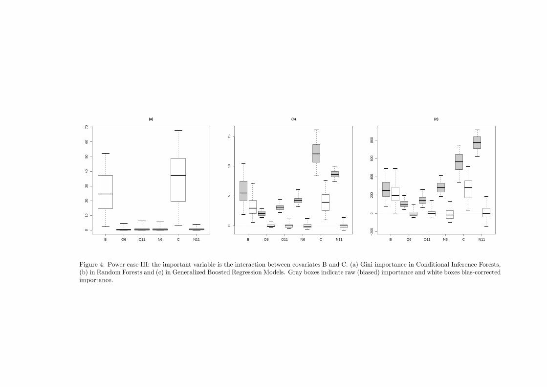
Power case III: the interaction of B and C is informative; the data generating process is defined as follows:

P (Y = 1|B = 1 ∩ C > 0) = 0.75 and P (Y = 1|B = −1 ∪ C ≤ 0) = 0.25.

We apply our bias correction method on two tree-based ensemble models: Random Forests and Gradient

Boosting Machine. We use the R packages randomForest and gbm. The number of trees for the two models

is T = 1000 and the minimum number of observations in the trees terminal nodes is 10. In randomForest

the number of variables randomly sampled as candidates at each split is mtry = 3. In gbm the maximum

depth of variable interactions is interaction.depth = 2 and the learning rate is shrinkage = 0.005. We

set the number of replications (without replacement) R defined in (5) to R = 100. For each simulation study

the number of samples analyzed is S = 100.

For comparison purpose, we compute the Gini importance of the 6 variables by the cforest command of

the party package of R ([Hothorn et al.(2006a)]). This command implements Random Forests and bagging

ensemble algorithms by utilizing conditional inference trees as base learners. The test statistic used is quad, a

univariate test statistics based on a quadratic form. The distribution of the test statistic has been computed

by the Bonferroni-adjusted method. The number of trees is T = 1000. Because the varimp command of this

package calculates only the measure of importance based on the mean decrease accuracy, we developed an

R function for the calculation of the Gini index in this class of models.

9

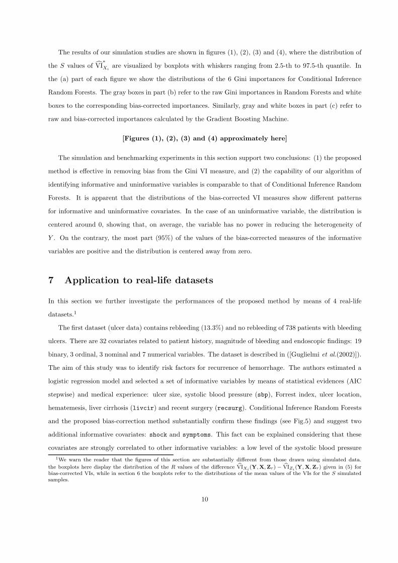
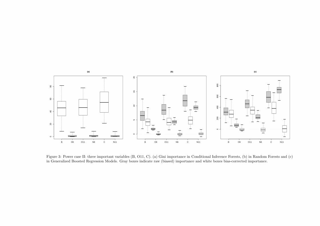
The results of our simulation studies are shown in figures (1), (2), (3) and (4), where the distribution of

the S values of VI∗

Xiare visualized by boxplots with whiskers ranging from 2.5-th to 97.5-th quantile. In

the (a) part of each figure we show the distributions of the 6 Gini importances for Conditional Inference

Random Forests. The gray boxes in part (b) refer to the raw Gini importances in Random Forests and white

boxes to the corresponding bias-corrected importances. Similarly, gray and white boxes in part (c) refer to

raw and bias-corrected importances calculated by the Gradient Boosting Machine.

[Figures (1), (2), (3) and (4) approximately here]

The simulation and benchmarking experiments in this section support two conclusions: (1) the proposed

method is effective in removing bias from the Gini VI measure, and (2) the capability of our algorithm of

identifying informative and uninformative variables is comparable to that of Conditional Inference Random

Forests. It is apparent that the distributions of the bias-corrected VI measures show different patterns

for informative and uninformative covariates. In the case of an uninformative variable, the distribution is

centered around 0, showing that, on average, the variable has no power in reducing the heterogeneity of

Y . On the contrary, the most part (95%) of the values of the bias-corrected measures of the informative

variables are positive and the distribution is centered away from zero.

7 Application to real-life datasets

In this section we further investigate the performances of the proposed method by means of 4 real-life

datasets.1

The first dataset (ulcer data) contains rebleeding (13.3%) and no rebleeding of 738 patients with bleeding

ulcers. There are 32 covariates related to patient history, magnitude of bleeding and endoscopic findings: 19

binary, 3 ordinal, 3 nominal and 7 numerical variables. The dataset is described in ([Guglielmi et al.(2002)]).

The aim of this study was to identify risk factors for recurrence of hemorrhage. The authors estimated a

logistic regression model and selected a set of informative variables by means of statistical evidences (AIC

stepwise) and medical experience: ulcer size, systolic blood pressure (sbp), Forrest index, ulcer location,

hematemesis, liver cirrhosis (livcir) and recent surgery (recsurg). Conditional Inference Random Forests

and the proposed bias-correction method substantially confirm these findings (see Fig.5) and suggest two

additional informative covariates: shock and symptoms. This fact can be explained considering that these

covariates are strongly correlated to other informative variables: a low level of the systolic blood pressure

1We warn the reader that the figures of this section are substantially different from those drawn using simulated data.

the boxplots here display the distribution of the R values of the difference VIXi(Y, X, Zr) − VIZi

(Y, X, Zr) given in (5) forbias-corrected VIs, while in section 6 the boxplots refer to the distributions of the mean values of the VIs for the S simulatedsamples.

10

is one of the clinical sign of shock and symptoms is a nominal variables with the following 4 categories:

melena, hematemesis, hematemesis+melena, other. Furthermore, in 4 numerical covariates (age, heart rate

hr, haematocrit ht and haemoglobin level hb) the effects of the bias of the Gini measure appeared more

pronounced and dangerous. These covariates show high values of the raw VI and, after bias removal, they

became uninformative or slightly informative.

The Hepatitis dataset is available at the UCI Machine Learning Repository and it contains survival

(79.3%) and nonsurvival of 155 chronic hepatitis patients with 19 covariates (13 binary and 6 numerical).

The covariates protime, alk phosphate and albumin are characterized by high percentage of missing values:

43%, 19% and 11%, respectively. Using a three-steps procedure based on forward logistic regression, the

Gregory’s rule described in [Gong (1986)] identified 4 predictive covariates: albumin, spiders, bilirubin and

sex. [Kim and Loh(2001)] estimated classification trees with binary and multiway splits (CART, QUEST,

CRUISE 1D and CRUISE 2D) finding that the top three predictors are protime, bilirubin, and albumin.

[Breiman(2001b)] calculated variable importance in Random Forests by the reduction of predictive accuracy

after random permutation of covariates and concluded that virtually all the predictive capability is provided

by a single variable (either ascites or albumin). Our analysis evidences that the most important covariates

are albumin, protime, ascites, histology and bilirubin (Fig.6). These results partially confirm the findings of

the preceding analyses and shed light on the role of a neglected covariate: histology. Conditional Inference

Forests and the unbiased Gini VI in Random Forests show that the importance of this variable is comparable

to that of ascites and bilirubin. The estimation of the out-of-bag prediction error of a Random Forest with

and without histology (the other covariates considered are albumin, ascites and bilirubin) indicate a moderate

predictive power of this covariate: 18.7% vs. 20.0%. Another interesting result evidenced by our analysis is

the marked level of bias in the Gini VI measure for the numerical covariates age, agot and alk phosphate.

Evaluating the Gini VI measure without bias correction would lead to a misleading attribution of importance

to these uninformative covariates.

[Figures (5) and (6) approximately here]

8 Concluding remarks

The Gini VI measure is frequently used in classification trees and in tree-based learning ensembles. This

measure has long been recognized by many authors to be affected by bias. The main consequence of this

systematic deviation is that variable selection may be influenced by covariate characteristics other than

information content. In spite of this potentially dangerous effect, the Gini index is often set as the default

VI measure in many software for data mining, without any correction.

11

In the present paper we proposed a bias correction heuristic strategy and investigated its performances

both on simulated and real data. The idea behind the algorithm is to artificially add a set of uninformative

pseudovariables to the original data whose VIs, under certain conditions, can approximate the unknown bias.

The results show that the method is capable of efficiently removing bias in many practical circumstances. In

addition, there is substantial agreement between our algorithm and the unbiased variable selection method

of [Hothorn et al.(2006a)].

Although the paper is focused on classification trees with the Gini gain as splitting criterion, preliminary

investigations give indications that the proposed strategy is also effective in regression trees and can be

extended to other heterogeneity measures (e.g. entropy-based measures). Another attractive advantage of

our method is that it can be easily integrated with minor efforts into any traditional algorithm for recursive

partitioning and might thus prove manageable and useful to applied scientists.

9 Acknowledgements

We are grateful to the Editor and two anonymous referees for their valuable comments and suggestions for

improving the quality of the paper. A special thank to Roberto Perli and Samantha Sartori for their help.

The usual disclaimer applies.

References

[Bell and Wang(2000)] Bell, D. and Wang, H. (2000): A formalism for relevance and its application in

feature subset selection. Machine Learning, 4(2), 175–195

[Breiman(2001a)] Breiman, L. (2001): Random Forests. Machine Learning, 45, 5–32.

[Breiman(2001b)] Breiman, L. (2001): Statistical Modeling: The Two Cultures Statistical Science, 16 (3),

199–231.

[Breiman(2002)] Breiman, L. (2002): Manual on setting up, using, and understanding Random Forests v3.1.

Technical Report, ftp://ftp.stat.berkeley.edu/pub/users/breiman/Using random forests v3.1.pdf.

[Breiman et al.(1984)] Breiman, L., Friedman, J.H., Olshen, R.A. and Stone, C.J. (1984): Classification and

Regression Trees. Chapman & Hall, London.

[Breiman et al.(2006)] Breiman L, Cutler A, Liaw A, Wiener M (2006): Breiman and Cut-

lers Random Forests for Classification and Regression. R package version 4.5-18 http://cran.r-

project.org/doc/packages/randomForest.pdf

12

[Bureau et al.(2003)] Bureau, A., Dupuis, J., Hayward, B., Falls, K. and Van Eerdewegh, P.

(2003): Mapping complex traits using Random Forests. BMC Genetics, 4(Suppl.1):S64,

http://www.biomedcentral.com/1471-2156/4/s1/S64

[Cummings and Myers(2004)] Cummings M.P. and Myers D.S. (2004): Simple statistical mod-

els predict C-to-U edited sites in plant mitochondrial RNA. BMC Bioinformatics, 5, 132,

http://www.biomedcentral.com/1471-2105/5/132

[De’ath(2007)] De’ath, G. (2007): Boosted trees for ecological modeling and prediction. Ecology, 88(1),

243–251.

[Dıaz-Uriarte and Alvarez de Andres(2006)] Dıaz-Uriarte, R. and Alvarez de Andres, S. (2006): Gene

selection and classification of microarray data using random forest. BMC Genetics, 7:3,

http://www.biomedcentral.com/1471-2105/7/3

[Dobra and Gehrke(2001)] Dobra A, Gehrke J (2001): Bias Correction in Classification Tree Construc-

tion. In Proceedings of the Seventeenth International Conference on Machine Learning, Williams College,

Williamstown, MA, USA. Edited by Brodley CE, Danyluk AP, pp. 90-97.

[Friedman(2001)] Friedman, J.H. (2001): Greedy function approximation: a gradient boosting machine.

Annals of Statistics, 29, 1189–1232.

[Friedman(2002)] Friedman, J.H. (2002): Tutorial: getting started with MART in R. Technical Report,

Standford University, http://www-stat.stanford.edu/ jhf/r-mart/tutorial/tutorial.pdf.

[Friedman et al.(2001)] Friedman, J.H., Hastie, T. and Tibshirani, R. (2001): The Elements of Statistical

Learning; Data Mining, Inference and Prediction. Springer, New York.

[Friedman and Meulman(2003)] Friedman, J.H. and Meulman, J.J. (2003): Multiple additive regression

trees with application in epidemiology. Statistics in Medicine, 22, 1365–1381.

[Gong (1986)] Gong, G. (1986): Cross-Validation, the Jackknife, and the Bootstrap: Excess Error Estima-

tion in Forward Logistic Regression. Journal of the American Statistical Association, 81(393), 108–113.

[Guglielmi et al.(2002)] Guglielmi, A., Ruzzenente, A., Sandri, M., Kind, R., Lombardo, F., Rodella, L.,

Catalano, F., De Manzoni, G. and Cordiano, C. (2002): Risk assessment and prediction of rebleeding in

bleeding gastroduodenal ulcer. Endoscopy, 34, 771–779.

13

[Guha and Jurs(2004)] Guha, R. and Jurs, P.C. (2004): Development of Linear, Ensemble, and Nonlinear

Models for the Prediction and Interpretation of the Biological Activity of a Set of PDGFR Inhibitors. J.

Chem. Inf. Comput. Sci., 44, 2179–2189.

[Hothorn et al.(2006a)] Hothorn, T., Hornik, K. and Zeileis, A. (2006): Unbiased Recursive Partitioning: A

Conditional Inference Framework. Journal of Computational and Graphical Statistics, 15 (3), 651–674.

[Hothorn et al.(2006b)] Hothorn, T., Hornik K., Zeileis, A. (2006): party: A Laboratory for Recursive

Part(y)itioning. R package version 0.9-11. http://cran.r-project.org/doc/vignettes/party/party.pdf

[John et al.(1994)] John, G.H., Kohavi, R., and Pfleger, K. (1994): Irrelevant features and the subset

selection problem. In: Cohen, W.W. and Hirsch, H. (eds), Proceedings of the 11th international conference

on machine learning, Morgan Kaufmann, New Brunswick, NJ, 121-129.

[Kim and Loh(2001)] Kim H., Loh W. (2001): Classification Trees with Unbiased Multiway Splits. Journal

of the American Statistical Association, 96, 589-604.

[Kononenko(1995)] Kononenko I. (1995): On Biases in Estimating Multi-Valued Attributes. In Proceedings

of the Fourteenth International Joint Conference on Artificial Intelligence, Montreal, Canada. Edited by

Mellish C., 1034-1040.

[Loh and Shih(1997)] Loh, W.-Y., Shih, Y.-S. (1997): Split selection methods for classification trees. Statis-

tistica Sinica, 7, 815–840.

[Lunetta et al.(2004)] Lunetta, K.L., Hayward, B.L., Segal, J. and Van Eerdewegh, P. (2004): Screening

large-scale association study data: exploiting interactions using random forests. BMC Genetics, 5:32,

http://www.biomedcentral.com/1471-2156/5/32

[Menze et al.(2007)] Menze, B.H., Petrich, W. and Hamprecht F.A. (2007): Multivariate feature selec-

tion and hierarchical classification for infrared spectroscopy: serum-based detection of bovine spongiform

encephalopathy. Anal. Bioanal. Chem., doi:10.1007/s00216-006-1070-5.

[Pearl(1988)] Pearl J. (1988): Probabilistic reasoning in intelligent systems: networks of plausible inference.

Morgan Kaufmann Publishers, Inc., San Francisco, California.

[Ridgeway(2007)] Ridgeway, G. (2007): Generalized Boosted Models: A guide to the gbm package. http://i-

pensieri.com/gregr/papers/gbm-vignette.pdf

[Ripley(1996)] Ripley, B. (1996): Pattern Recognition and Neural Networks. Cambridge University Press,

Cambridge

14

[Schonlau(2005)] Schonlau, M. (2005): Boosted Regression (boosting): A Tutorial and a Stata plugin. The

Stata Journal, 5(3), 330–354.

[Strobl(2005)] Strobl, C. (2005): Statistical Sources of Variable Selection Bias in Classifi-

cation Trees Based on the Gini Index. Technical Report, SFB 386, http://epub.ub.uni-

muenchen.de/archive/00001789/01/paper 420.pdf

[Strobl et al.(2007a)] Strobl, C., Boulesteix, A.-L., Zeileis, A. and Hothorn, T. (2007): Bias in Random

Forest Variable Importance Measures: Illustrations, Sources and a Solution. BMC Bioinformatics, 8:25,

doi:10.1186/1471-2105-8-25

[Strobl et al.(2007b)] Strobl, C., Boulesteix, A.-L. and Augustin, T.(2007): Unbiased split selec-

tion for classification trees based on the Gini Index. Computational Statistics & Data Analysis,

doi:10.1016/j.csda.2006.12.030

[Svetnik et al.(2005)] Svetnik, V., Wang, T., Tong, C., Liaw, A., Sheridan, R.P. and Song Q. (2005): Boost-

ing: An Ensemble Learning Tool for Compound Classification and QSAR Modeling. J. Chem. Inf. Model.,

45, 786–799

[White and Liu(1994)] White, A.P. and Liu, W.Z. (1994): Bias in Information-Based Measures in Decision

Tree Induction. Machine Learning, 15, 321–329.

[Wu et al.(2007)] Wu, Y., Boos, D.D. and Stefanski, L.A.(2007): Controlling Variable Selection by the

Addition of Pseudovariables. Journal of the American Statistical Association, 102 (477), 235–243.

[Yu and Liu(2004)] Yu, L. and Liu, H. (2004): Efficient Feature Selection via Analysis of Relevance and

Redundancy. Journal of Machine Learning research, 5, 1205-1224.

15

B O6 O11 N6 C N11

01

23

45

6

(a)

B O6 O11 N6 C N11

02

46

810

(b)

B O6 O11 N6 C N11

050

010

0015

00

(c)

Figure 1: Null case: all uninformative variables. (a) Gini importance in Conditional Inference Forests, (b) in Random Forests and (c) in GeneralizedBoosted Regression Models. Gray boxes indicate raw (biased) importance and white boxes bias-corrected importance.

B O6 O11 N6 C N11

010

2030

4050

60

(a)

B O6 O11 N6 C N11

05

1015

(b)

B O6 O11 N6 C N11

−200

020

040

060

080

010

00

(c)

Figure 2: Power case I: the only important variable is B. (a) Gini importance in Conditional Inference Forests, (b) in Random Forests and (c) inGeneralized Boosted Regression Models. Gray boxes indicate raw (biased) importance and white boxes bias-corrected importance.

B O6 O11 N6 C N11

020

4060

80

(a)

B O6 O11 N6 C N11

05

1015

20

(b)

B O6 O11 N6 C N11

020

040

060

080

0

(c)

Figure 3: Power case II: three important variables (B, O11, C). (a) Gini importance in Conditional Inference Forests, (b) in Random Forests and (c)in Generalized Boosted Regression Models. Gray boxes indicate raw (biased) importance and white boxes bias-corrected importance.

B O6 O11 N6 C N11

010

2030

4050

6070

(a)

B O6 O11 N6 C N11

05

1015

(b)

B O6 O11 N6 C N11

−200

020

040

060

080

0

(c)

Figure 4: Power case III: the important variable is the interaction between covariates B and C. (a) Gini importance in Conditional Inference Forests,(b) in Random Forests and (c) in Generalized Boosted Regression Models. Gray boxes indicate raw (biased) importance and white boxes bias-correctedimportance.

sizeshockforrest

sbphematem

symptomsrecsurg

uobdhb

livciranticoag

hthr

location2crf

genderage

nsaidndrugs

pubpud

malignhyp

diabmelvascureum

nillnesspastsurg

bdhgastritis

location1nulcers

0.000

0.001

0.002

0.003

0.004

0.005

0.006

(a)

0 1 2 3 4 5

sbpsize

shockforrest

recsurghb

symptomshr

uobdhematem

htanticoaglocation2

livcirndrugs

gastritisnillness

crfbdh

malignreum

hyppastsurg

nsaidpub

gendernulcers

location1diabmel

vascupudage

0 1 2 3 4 5

(b)

−100 0

100

200

300

400

500

sizesbp

forrestrecsurg

hrlivcir

symptomshb

location2anticoag

hematemuobd

crfshock

gastritisnillness

bdhgender

agelocation1

malignhyp

htnulcersndrugs

reumdiabmel

vascupastsurg

pubpud

nsaid

−100 0

100

200

300

400

500

(c)

Fig

ure

5:

Ulcer

data

:(a

)G

iniim

porta

nce

inC

onditio

nalIn

ference

Forests,

(b)

inR

andom

Forests

and

(c)in

Gen

eralized

Boosted

Reg

ression

Models.

In(b

)and

(c)figures,

bars

indica

teraw

(bia

sed)

importa

nce

and

gray

box

esbia

s-corrected

importa

nce.

albumin

histology

ascites

protime

bilirubin

spiders

varices

alkphos

malaise

age

sex

steroid

antivirals

fatigue

anorexia

liverbig

liverfirm

spleen

sgot

0.000

0.002

0.004

0.006

0.008

0.010

0.012

0.014

(a)

−0.5

0.0

0.5

1.0

1.5

2.0

2.5

protime

albumin

ascites

bilirubin

histology

alkphos

varices

spiders

age

malaise

anorexia

spleen

liverbig

fatigue

steroid

sex

liverfirm

antivirals

sgot

−0.5

0.0

0.5

1.0

1.5

2.0

2.5

(b)

−40

−20 0 20 40 60 80

protime

histology

bilirubin

age

albumin

malaise

anorexia

varices

sex

ascites

liverbig

spiders

spleen

antivirals

alkphos

liverfirm

fatigue

steroid

sgot

−40

−20 0 20 40 60 80

(c)

Fig

ure

6:

Hep

atitis

data

:(a

)G

iniim

porta

nce

inC

onditio

nal

Inferen

ceForests,

(b)

inR

andom

Forests

and

(c)in

Gen

eralized

Boosted

Reg

ression

Models.

In(b

)and

(c)figures,

bars

indica

teraw

(bia

sed)

importa

nce

and

gray

box

esbia

s-corrected

importa

nce.