Option Pricing in a Black-Scholes Model with Markov Switching

Fuh, Cheng-Der1 and Wang, Ren-Her

Institute of Statistical Science, Academia Sinica, Taipei, Taiwan, R.O.C.

Cheng, Jui-Chi

Graduate Institute of Finance, National Taiwan University, Taipei, Taiwan, R.O.C.

ABSTRACT

The theory of option pricing in Markov volatility models has been developed in recent

years. However, an efficient method to compute option price in this setting remains

lacking. In this article, we present a way of modeling time-varying volatility; to generalize

the classical Black-Scholes model to encompass regime-switching properties. Specifically,

the unobserved state variables for stock fluctuations are governed by a first-order Markov

process, and the drift and volatility parameters take different values depending on the

state of this hidden Markov model. Standard option pricing procedure under this model

becomes problematic. We first provide a closed-form formula for the arbitrage-free price

of the European call option. In the case of the underlying Markov process has two

states, we have an explicit analytic formula for option price. When the number of states

for the underlying Markov process is bigger than two, we propose an approximation

formula for option price. The idea of the approximation formula is that we replace

the distribution of occupation time for a given state by its corresponding stationary

distribution multiplies the whole time period. Numerical methods, such as Monte-Carlo

simulation and Markovian tree, to compute European call option price are presented

for comparison. Our numerical results show that the approximation formula provide

an efficient and reliable implementation tool for option pricing. Implied volatility and

implied volatility surface are also given.

Keywords: Arbitrage, Black-Scholes model, European call option, hidden Markov model,

implied volatility, Laplace transform, Monte Carlo, tree.

1. Research partially supported by NSC 91-2118-M-001-016.

1

1. Introduction

It is well-known that the volatility of financial data series tends to change over time,

and changes in return volatility of stock returns tend to be persistent. The statistical

properties of return volatility have been deeply studied and uncovered in the financial

economic literatures, for instance, the extensive work on modeling stock fluctuations

with stochastic volatility (cf. Anderson, 1996; Hull and White, 1987; Stein, 1991; Wig-

gins, 1987; Heston, 1993), and uncertain volatility (Avellaneda, Levy, and Paras, 1995).

Many efforts have been made to study financial markets with different information levels

among investors (cf. Duffie and Huang, 1986; Ross, 1989; Anderson, 1996; Karatzas and

Pikovsky, 1996; Guilaume et. al., 1997; Grorud and Pontier, 1998; Imkeller and Weisz,

1999). Like the Markov switching model of Hamilton (1988, 1989) may provide more

appropriate modeling of volatility. In this regard, Hamilton and Susmel (1994) proposed

the Markov switching ARCH model. In a partial equilibrium model, Turner, Startz and

Nelson (1989) formulate a switching model of excess returns in which returns switch ex-

ogenously between a Gaussian low variance regime and a Gaussian high variance regime.

So, Lam and Li (1998) generalizes the stochastic volatility model to incorporate Markov

regime switching properties. Diebold and Inoue (2001) considers the properties of long

memory and regime switching.

In deed, recent research (cf. Bittlingmayer, 1998) has shown that investors’ un-

certainty over some important factors affecting the economy may greatly impact the

volatility of stock returns. More generally, there is evidence that investors tend to be

more uncertain about the future growth rate of the economy during recessions, thereby

partly justifying a higher volatility of stock returns. In this paper, to encompass the

empirical phenomena of the stock fluctuations relate to business cycle, we introduce a

model of an incomplete market by adjoining the Black-Scholes exponential Brownian

motion model for stock fluctuations with a hidden Markov process. Specifically, we

assume that stock of asset pricing are generated by realization of a Gaussian diffusion

process, and the drift and volatility parameters take different values depending on the

state of a hidden Markov process. That is, we assume that identical investors cannot

observe the drift rate, as well as the volatility of course, of the dividend process, but

they have to infer it from the observation of past dividends. We call this model a Black-

Scholes model with Markov switching, or a hidden Markov model in brief. Related works

in this type have been studied and documented in the literatures, for instance, Detemple

(1991) and David (1997) encompass the regime switching properties of the drift to the

classical Cox-Ingersoll-Ross model, while Veronesi (1999) studies the Gaussian diffusion

model. These papers focus on the issue of modeling stock returns and their empirical

phenomena. They also study investors’ optimal portfolio allocation and show that equi-

librium marketwise excess returns display changing volatility, negative skewness, and

negative correlation with future volatility.

2

For the concern of option pricing in Markov volatility models. Di Masi, Kabanov

and Runggaldier (1994) considers the problem of hedging an European call option for

a diffusion model where drift and volatility are function of a two state Markov jump

process. Guo (2001) also considers the same model and gives a closed-form formula for

the European call option. However, her formula is not appropriate stated and has a

mistake. The contribution of this paper is to give a closed-form formula in the case of

a two state hidden Markov model, and to propose an approximation formula for the

arbitrage-free price of the European call option in general case. The idea of the approxi-

mation formula is that we replace the distribution of occupation time for a given state by

its corresponding stationary distribution multiplies the whole time period. Numerical

methods, such as Monte-Carlo simulation and Markovian tree, to compute European

call option price are presented for comparison. Our numerical results show that the

approximation formula provide an efficient and reliable implementation tool for option

pricing.

This article is organized as follows. In Section 2, we first define the Black-Scholes

model with Markov switching that capture the phenomenon of business cycle in stock

fluctuations. Then, we provide a closed-form formula for the price of the European call

option, and in particular, we give an explicit analytic formula for option price when the

underlying Markov process has two states. In Section 3, we propose an approximation

formula for option price in a finite state hidden Markov model. To illustrate the perfor-

mance of the approximation formula, in Section 4, we presents numerical and simulation

results for comparison. These outcomes are reported in terms of Monte-Carlo simulation

and Markovian tree, respectively. Implied volatility and implied volatility surface are

also given to support our results. Section 5 is conclusions. The derivation of the option

price formula is in the Appendix.

2. The hidden Markov model and option price

We incorporate the existence of business cycle by modeling the fluctuations of a single

stock price Xt, using an equation of the form

dXt = Xtµε(t)dt+Xtσε(t)dWt, (1)

where ε(t) is a stochastic process representing the state of business cycle, Wt is the

standard Wiener process which is independent of ε(t). For each state of ε(t), the drift

parameter µε(t) and volatility parameter σε(t) are known, and take different values when

ε(t) is in different state.

We also assume that the supply of the risky asset is fixed and normalized to 1. The

risky free asset is supplied and has an instantaneous rate of return equal to r. Note that

3

this assumption not only simplify the analysis, in particular for option pricing, but also

matches the empirical finding that the volatility of the risk-free rate is much lower than

the volatility of market returns.

Assume that ε(t) is a Markov process with a few states (maybe two or three states).

In financial economic, we know that business cycle can divide into two different states

called expansion and contraction. A growing economy is described as being in expansion.

In this state, let ε(t) = 0, µε(t) = µ0 and σε(t) = σ0. On the other hand, we can take

the value ε(t) = 1, µε(t) = µ1 and σε(t) = σ1 to represent the state in contraction. More

generally, one can use the state space Ω = 0, 1, · · · , N for ε(t) to model more complex

business cycle structures. In this section, for simplicity, we consider a two state hidden

Markov model for a single stock price Xt by using an equation of (1), where ε(t) is a

Markov process representing the state. Let

ε(t) =

0, when the business cycle in expansion,1, when the business cycle in contraction.

Assume σ0 6= σ1.

For the concern of the transition rate, let λi be the rate of leaving state i, and τi the

time of leaving state i. We assume that

P (τi > t) = e−λit, i = 0, 1.

Then the memoryless property of this process is plausible in that, from a practical

standpoint, the information flow be identified more easily otherwise.

It is conceivable that sometimes investors will try to manipulate their buying and

selling in such a way that the existence of such information is not detectable from the

change of volatilities, namely σ are identical, see Detemple (1991), David (1997), and

Veronesi (1999). The problem of detecting the state change of ε(t) when σ remain

unchanged appears to be hard to solve mathematically. It is plausible that change in

business cycle distribution, hence predictability, manifests itself in the diffusion coeffi-

cient in the form of both stochastic volatility and drift. If we assume that the σ are

distinct then it is no loss of generality to assume that ε(t) is actually observable, since

the local quadratic variation of Xt in any small interval to the left of t will yield σε(t)

exactly. (For details, see McKean, 1969.) Hence, even if Xt is not Markovian, the joint

distribution (Xt, ε(t)) is so.

Despite the success of the classical Black-Scholes model, some empirical phenom-

ena have received much attention recently. An important assumption in the Black-

Scholes model is that the underlying asset distribution is assumed to be Normal, and

the volatility is a fixed constant. However, empirical evidences suggest that it has clus-

ter phenomenon, leptokurtic and unsymmetrical feature. Due to the adjoin of the stock

4

fluctuations with a hidden Markov process (the drift and volatility parameters take dif-

ferent values depending on the state of this hidden Markov process) in the Black-Scholes

exponential Brownian motion model, David (1997) shows that model (1) displays the

asymmetric leptokurtic features, negative skewness, and negative correlation with future

volatility. Veronesi (1999) shows that model (1) is better than the Black-Scholes model

to explain features of stock returns, including volatility clustering, leverage effects, ex-

cess volatility and time-varying expected returns. They both show that model (1) can

be embedded into a rational expectation equilibrium framework. For the concern of the

empirical phenomenon on volatility smile, we will present implied volatility and implied

volatility surface in the end of Section 4.

To get the option price formula, we know model (1) is arbitrage-free but incomplete

(cf. Harrison and Pliska (1981), Harrison and Kreps (1979)). One way to treat this

situation can be found in Follmer and Sondermann (1986), and Schweizer (1991), based

on the idea of hedging under a mean-variance criterion. Here, we follow the method by

D. Duffie to complete the market: at each time t, there is a market for a security that

pays one unit of account (say, a dollar) at the next time τ(t) = infu > t|ε(u) 6= ε(t)that the Markov chain ε(t) changes state. One can think of this as an insurance contract

that compensates its holder for any losses that occur when the next state change occurs.

Of course, if one wants to hedge a given deterministic loss C at the next state change,

one holds C of the current change-of-state (COS) contracts. For the detail, see Guo

(2001). It can be shown that the absence of arbitrage is effectively the same as the

existence of a probability Q, equivalent to P , under which the price of any derivative is

the expected discounted value of its future cash flow.

The same exercise applied to the underlying risky-asset implies that its price process

X must have the formdXt

Xt= (r − dε(t))dt+ σε(t)dW

Qt , (2)

where WQt is the standard Brownian motion under the risk-neutral probability Q, and

dε(t) = r − µε(t). Note that dε(t) is the cost of change of state at the time t. When the

state change at time t, the drift is different from the riskless interest rate r by d0 − d1,

and the arbitrage opportunity emerges at this moment.

Denote Ti as the total time between 0 and T during which ε(t) = 0, starting from

state i for i = 0, 1. Let fi(t, T ) be the probability distribution function of Ti.

Theorem 1 Under hidden Markov model (1). Given Equation (2), COS, and riskless

interest rate r, the arbitrage free price of a European call option with expiration date T

and strike price K is

Vi(T,K, r) = E[e−rT (XT −K)+|ε(0) = i]

5

= e−rT∫ ∞

0

∫ T

0

y

y +Kρ(ln(y +K), m(t), v(t))fi(t, T )dtdy, (3)

where ρ(x,m(t), v(t)) is the normal density function with expectation m(t) and variance

v(t),

m(t) = ln(X0) + (d1 − d0 −1

2(σ2

0 − σ21))t+ (r − d1 −

1

2σ2

1)T,

v(t) = (σ20 − σ2

1)t+ σ21T,

and

ρ(x,m(t), v(t)) =1

√

2πv(t)exp

− (x−m(t))2

2v(t)

,

f0(t, T ) = e−λ0T δ0(T − t) + e−λ1(T−t)−λ0t[λ0I0(2(λ0λ1t(T − t))1/2)

+(λ0λ1t

T − t)1/2I1(2(λ0λ1t(T − t))1/2)], (4)

f1(t, T ) = e−λ1T δ0(T − t) + e−λ1(T−t)−λ0t[λ1I0(2(λ0λ1t(T − t))1/2)

+(λ0λ1(T − t)

t)1/2I1(2(λ0λ1t(T − t))1/2)], (5)

where I0 and I1 are modified Bessel functions such that

Ia(z) = (z

2)a

∞∑

k=0

(z/2)2k

k!Γ(k + a+ 1)!.

Remarks: 1. When µ0 = µ1, σ0 = σ1, m(t) and v(t) are independent of t and

Equation (3) reduces to the classical Black-Scholes formula for European call options.

2. By using the properties of order statistics, Di Masi, Kabanov and Runggaldier

(1994) obtains the distribution of the Kac process, which is a key step for option pricing

in a two state hidden Markov model. In this paper, we apply the method of Laplace

transform to get the distribution. The proof of Theorem 1 will be given in the Appendix.

3. Option pricing under a finite state hidden Markov

model

In this section, we extend our results to a finite state hidden Markov model. When

the number of states is two, Equation (3) gives a closed-form formula of the European

call option price, and Equations (4) and (5) provide the explicit form to compute the

distributions of the occupation times. Note that the idea of duality to compute fi(t, T )

for i = 0, 1 in a two state hidden Markov process can not be applied to general states,

and the computation of the probability distribution function fi(t, T ) with three or more

6

states becomes complicated and infeasible. However, detailed observation of Equation

(3) reveals that there are two important features in the option price formula. First, it

depends only the occupation time Ti, but not depend on the sample path of visiting each

particular state. Secondly, Equation (3) is valid in no respect to the number of states.

Therefore, instead of direct computation of fi(t, T ) as those in Equations (4) and (5),

we can approximate Ti as follows: Note that Ti/T → πi in probability as T → ∞ for

any finite state ergodic Markov process, hence we can give an approximation formula by

simply substituting Ti in Equation (3) by πiT . Since the expiration time T for a market

option is half to one year, the approximation should be accurate enough in such time

period.

In the case of a two state hidden Markov model, we also have the following empirical

evidence. Note that in Equations (3) to (5), there are two different states, 0 and 1, and

the option prices depend on the initial state. To the extremely case, we may consider the

situation to which the state is the same in whole time period. That is, the price given by

the classical Black-Scholes models at state 0 (or at state 1), respectively. For example, in

Figure 1, the dash lines represent the option prices given by the classical Black-Scholes

model for each given state, and the real lines represent the prices by Equation (3). Note

that the option prices by Equation (3) are within the two classical Black-Scholes models

and converge to a fixed option price when T is large enough. This empirical phenomenon

also provide the rational of the approximation formula for large enough time period.

Figure 1: Option pricing with Black-Scholes model and two state hidden Markov model.The parameter values: X0 = 100, K = 110, λ0 = λ1 = 10, d0 = d1 = 0, r = 0.1, σ0 =0.2, σ1 = 0.3.

Next, we will explain how to compute the stationary distribution π as follows: Let

ε(t), t ≥ 0 be the underlying continuous time Markov process in (1). Denote the

7

transition probability from state i to state j in the time period t as

pt(i, j) = P (ε(t) = j|ε(0) = i).

Let

q(i, j) = limh→0

ph(i, j)

h

be the jump rates for i 6= j. We have the stationary distribution π by solving the balance

equation πQ = 0, where Q is the matrix of transition rates

Q(i, j) =

q(i, j) j 6= i,−λi j = i,

where λi =∑

j 6=i q(i, j) is the total rate of transitions out of state i.

As the expiration date T tends to infinity, Equations (4) and (5) become

f0(t, T ) = f1(t, T ) =

0, when t = T,1, when t 6= T.

(6)

Therefore the approximation formula of Equation (3) in Theorem 1 can be written as

Vi (7)

= e−rT∫ ∞

0

y

y +K(ρ(ln(y +K), m(π0T ), v(π0T ))(1− e−λ0T δ0(i− 0)− e−λ1T δ0(1− i))

+ρ(ln(y +K), m(T ), v(T ))e−λ0T δ0(i− 0)) + ρ(ln(y +K), m(0), v(0))e−λ1T δ0(1− i))dy.

Figure 2 displays option prices under the same parameters. The dash lines represent

the prices given by the approximation formula (7), and the real lines represent the prices

given by Equation (3) under different initial state. We note that two dash lines are very

close to the two real lines, and they are within the two real lines. Hence they will

converge to the fixed option price faster than the real lines. The reason to describle this

phenomenon is simply that we use the stationary distribution π in (7).

By using the same idea as that in (7), we have the approximation formula for Euro-

pean call option in hidden Markov model ε(t) with finite state space Ω = 0, 1, · · · , Nas

Vi = e−rT∫ ∞

0

y

y +K(ρ(ln(y +K), m(t0, t1, · · · , tN), v(t0, t1, · · · , tN))

(1− e−λ0T δ0(0− i)− · · · − e−λN T δ0(N − i))

+ρ(ln(y +K), m(T, 0, · · · , 0), v(T, 0, · · · , 0))e−λ0T δ0(0− i) + · · ·+ρ(ln(y +K), m(0, 0, · · · , T ), v(0, 0, · · · , T ))e−λN T δ0(N − i))dy, (8)

8

! "# $ %

!

#

$

&'()&+* '-,)./

Figure 2: Option pricing for a two states hidden Markov model. The parameter values:X0 = 100, K = 110, λ0 = λ1 = 1, d0 = d1 = 0, r = 0.1, σ0 = 0.2, σ1 = 0.3.

where ti = πiT , i = 0, · · · , N and

m(t0, t1, · · · , tN) = ln(X0) +N

∑

i=0

(r − di −1

2σ2

i )ti,

v(t0, t1, · · · , tN) =N

∑

i=0

σ2i ti.

In practice, a three state hidden Markov chain is good enough to capture the empir-

ical phenomena of most financial data series, and the computational method is the same

for each finite state Markov process. Hence, we only consider the case of three state

hidden Markov model in our simulation study. Figure 3 displays option prices under the

same parameters. Here, the dash lines represent the prices given by the approximation

formula, and the real lines represent the prices given by Black-Scholes formula under dif-

ferent initial state. In principle, the number of states exceed three can be implemented

in the same matter, but to discriminate and find out the matrix of transition rates Q in

some time interval might be computational demanding.

9

0213 0214 0215 0216 7 8

3

4

5

6

7-0

739:;=<=9> :@?-<=ACB

Figure 3: Option pricing for a three states hidden Markov model. The parameter values:X0 = 100, K = 110, λ0 = λ1 = λ2 = 10, d0 = d1 = d2 = 0, r = 0.1, σ0 = 0.1, σ1 =0.2, σ2 = 0.3.

4. Numerical performance

4.1 Design of the simulation

Numerical performance of the approximation formula (8) for option pricing is presented

in this section. We compare European call option prices obtained by Monte-Carlo sim-

ulation, Markovian tree method and the approximation formula. Two state and three

state hidden Markov models are considered in the simulation study, respectively. The

performance of this comparison is based on the “difference” of the option prices. The

definition of difference will be given later. We use the exact analytic formula as the

benchmark in the case of a two state hidden Markov model, and the Monte-Carlo sim-

ulation result as the benchmark in the case of a three state hidden Markov model. The

results are shown in Tables 1 to 10, in which four factors are used:

(1) Low and high volatilities.

(2) Different transition rates in the case of a three state hidden Markov model.

(3) Different strike prices. Specifically, we consider the cases of in the money, at the

money and out of the money.

(4) Different expiration date; T = 0.1, 0.2, 0.5, 1, 2, 3, with unit of year.

Since model (1) is a continuous time model, we discretize this continuous time model

in the vein of Cox, Ross, and Rubinstein (1979). A corresponding two state hidden

Markov model based on Cox, Ross and Rubinstein (1979) can be found in David (1997).

It is worth pointing out that this methodology applies also to the general case where

the hidden Markov process ε(t) takes more than three states, i.e., the state space can

10

be Ω = 0, 1, · · · , N, when, for example, more complex information patterns can be

imposed.

We can apply Equation (2) for Monte-Carlo simulation of the option price. First,

rewrite Equation (2) in the discrete time form

Xn+h = Xne(r−

1

2σ2

εn− dεn

)h+ σεn

√hη, (9)

where η is simulated from the standard normal random variable N(0, 1). Second, con-

sider the random variable εn with transition probability of changing state by (δi,j +

(−1)δi,je−q(i,i)h)(|q(i, j)/λi|). Repeat the steps for M times, where M is large enough to

guarantee the convergence of the simulation.

To illustrate the idea of discretization in Markovian tree method, we first construct

the structure of a two state hidden Markov model as follows: Suppose the time interval

[0, t] is divided into n sub-intervals such that t = nh. Let X = (Xk, k ≥ 0) and Xk is a

price at time kh. Define

Xεk

k = (Xk, εk) = (X(kh), ε(kh)).

Let ηi,jn be independent and identically distributed (i.i.d.) random variables, taking

values uj with probability pj(δi,1−j + (−1)δi,1−je−λih), and 1/uj with probability (1 −pj)(δi,1−j + (−1)δi,1−je−λih), i, j = 0, 1, respectively, where

ui = eσi

√h, pi =

µih + σi

√h− 0.5σ2

i h

2σi

√h

.

Then, we have the following recurrence relation,

(Xn, εn) = ηε(n),ε(n−1)n (Xn−1, εn−1). (10)

By the memoryless property of τi, (Xεnn , n ≥ 0) is a Markov chain. The Markov chainXεn

n

with initial state X0 = x is a random walk on the set Ex = xur|r = σ0n0+σ1n1, n0, n1 ∈Z, u = e

√h.

In general, we can apply the same idea to the hidden Markov model with state

space Ω = 0, 1, · · · , N. Denote Q as the matrix of transition rates. Note that the

ηi,jn in Equation (9) are independent and identically distribute random variables, taking

values uj with probability pj(δi,j+(−1)δi,je−q(i,i)h)(|q(i, j)/λi|), and 1/uj with probability

(1 − pj)(δi,j + (−1)δi,je−q(i,i)h)(|q(i, j)/λi|), where i represents the current state and j

represents the oncoming state in one sub-interval. Similarly, the Markov chain X εnn with

initial state X0 = x is a random walk on the set Ex = xur|r = σ0n0 + σ1n1 + · · · +σNnN , n0, n1, · · · , nN ∈ Z, u = e

√h.

11

Here we consider n, the number of sub-interval, to be 30, since our simulation

shows that this number is large enough to provide accurate results. The Monte-Carlo

replication size for both Monte-Carlo simulation and Markovian tree method is B =

50, 000, 000. Computations were performed using Visual Basic programs on the personal

computer system with a Pentium 4 CPU, 1.6G and 256MB of RAM, of the Institute

of Statistical Science, Academia Sinica, Taipei, Taiwan, R.O.C.. The pseudo-random

numbers were generated by using IMSL routines. All tests were compared on the basis of

the same random numbers, samples of different size were nested. The reported running

time is given the CPU time in seconds.

4.2 Simulation results

We will use the following abbreviations in Tables 1 to 10. B-S i refers to the clas-

sical Black-Scholes formula with state i = 0, 1; Vi refers to the exact price of a two

state hidden Markov model; Vi refers to the approximation price of a two states hidden

Markov model; sim i and tree i refer to Monte-Carlo simulation for Equation (2) and

Markovian tree method, respectively.

We first consider the case of a two state hidden Markov model, with the same

transition rates. Tables 1 and 2 report the numerical and simulation results according

to low and high volatilities. The other parameters are the same. Note from Tables 1 and

2 that the numerical values given by the Monte-Carlo simulation and the Markov tree

method are very close to the same values for various time period. In the case of short

time period, the performance of the approximation formula is better than Monte-Carlo

simulation and Markovian tree method, in the sense to compare the results obtained

by the exact formula. And the computational time is reduced significantly. Therefore,

the approximation formula (7) gives a rather promising result in the case of a two state

hidden Markov model.

Table 1: The parameters are: X0 = 100, K = 90, λ0 = λ1 = 1, d0 = d1 = 0, r =0.1, σ0 = 0.2, σ1 = 0.3, n = 30.

T (year) B-S 0 B-S 1 V0 V1 sim 0 sim 1 tree 0 tree 1 V0 V1

0.1 10.975 11.381 10.993 11.360 10.986 11.346 10.910 11.314 10.993 11.3600.2 12.088 12.968 12.164 12.889 12.151 12.883 12.257 12.698 12.166 12.8860.5 15.288 17.034 15.614 16.718 15.592 16.719 15.497 16.960 15.639 16.6981.0 19.988 22.510 20.721 21.812 20.681 21.796 20.740 21.747 20.811 21.7392.0 28.037 31.281 29.287 30.085 29.256 30.051 29.166 30.060 29.478 29.9173.0 34.996 38.504 36.476 37.061 36.426 37.057 36.219 36.877 36.689 36.863

runningtime(sec) < 10−5 < 10−5 1.51 1.45 240.55 251.32 140.24 144.23 0.061 0.063

12

Table 2: The parameters are: X0 = 100, K = 90, λ0 = λ1 = 1, d0 = d1 = 0, r =0.1, σ0 = 0.1, σ1 = 1.0, n = 30.

T (year) B-S 0 B-S 1 V0 V1 sim 0 sim 1 tree 0 tree 1 V0 V1

0.1 17.007 18.100 17.059 18.050 17.048 18.045 16.842 18.050 17.060 18.0500.2 21.612 23.180 21.752 23.045 21.731 23.050 21.860 23.135 21.757 23.0420.5 31.027 33.429 31.478 32.996 31.468 32.994 31.765 32.995 31.513 32.9691.0 41.547 44.688 42.460 43.818 42.455 43.760 42.662 44.106 42.570 43.7262.0 55.470 59.236 56.934 57.858 56.945 57.871 56.817 57.616 57.158 57.6683.0 64.952 68.853 66.638 67.286 66.671 67.415 66.080 66.550 66.884 67.078

runningtime(sec) < 10−5 < 10−5 1.44 1.52 249.46 252.55 100.23 101.17 0.060 0.063

Let Q1 be the matrix of transition rate

Q1 =

−1 1 01/2 −1 1/20 1 −1

,

and let Q2 be the matrix of transition rate

Q2 =

−1 1 05/2 −5 5/20 10 −10

.

The results of a three state hidden Markov model are recorded in Tables 3 to 6. Note

that the matrix of transition rates Q is the same for a two state hidden Markov model;

while the matrix of transition rates Q may be different in a three or more state hidden

Markov models. Since the difference of the matrix of transition rates in a three or more

states hidden Markov model may also play an important role for option pricing, we will

present our simulation results accordingly. Tables 3 and 4 displays the option prices for

a three states hidden Markov model, with matrix of transition rate Q1 (with the same

transition rate), the same parameters, but different volatilities. Tables 5 and 6 displays

the option prices for a three states hidden Markov model, with matrix of transition rate

Q2 (with different transition rate), the same parameters, but different volatilities.

Note from Tables 3 to 6 that we have three numerical consequences. First, the

option prices obtained by the approximation formula (8) are less sensitive to the initial

state than those obtained by Monte-Carlo simulation and Markovian tree method. The

rational behind this phenomenon is that we use the stationary distribution π, instead of

exactly probability distribution, in the approximation formula (8). Secondly, the option

prices in Tables 5 and 6 with bigger λi values, i.e. λ1 and λ2, are closer to the values given

by the Monte-Carlo simulations than the price with λ0. This result is reasonable, since

13

Table 3: The parameters are: X0 = 100, K = 90, λ0 = λ1 = λ2 = 1, d0 = d1 = d2 =0, r = 0.1, σ0 = 0.1, σ1 = 0.2, σ2 = 0.3, n = 30.

T (year) sim 0 sim 1 sim 2 tree 0 tree 1 tree 2 V0 V1 V2

0.1 10.898 10.973 11.346 10.904 10.988 11.309 10.906 10.978 11.3450.2 11.806 12.078 12.886 11.840 12.199 12.694 11.854 12.103 12.8230.5 14.572 15.282 16.721 14.639 15.084 17.050 14.833 15.358 16.4171.0 19.061 19.978 21.761 18.987 20.167 21.744 19.656 20.155 21.0832.0 27.201 28.028 29.736 27.067 27.409 29.776 28.103 28.327 28.7663.0 34.333 34.953 36.426 34.057 34.667 36.386 35.250 35.331 35.506

runningtime(sec) 269.25 272.84 276.63 171.25 175.22 178.32 0.061 0.062 0.061

Table 4: The parameters are: X0 = 100, K = 90, λ0 = λ1 = λ2 = 1, d0 = d1 = d2 =0, r = 0.1, σ0 = 0.8, σ1 = 0.9, σ2 = 1.0, n = 30.

T (year) sim 0 sim 1 sim 2 tree 0 tree 1 tree 2 V0 V1 V2

0.1 15.984 16.993 18.021 15.683 16.797 18.025 16.036 17.010 17.9990.2 20.170 21.584 23.062 20.105 21.725 23.145 20.344 21.620 22.9040.5 29.118 31.025 32.906 29.027 31.345 32.939 29.590 31.053 32.5101.0 39.464 41.555 43.674 39.726 42.048 43.887 40.427 41.602 42.7582.0 53.760 55.456 57.202 53.621 56.074 57.049 55.033 55.563 56.0723.0 63.782 64.822 66.494 63.304 64.395 65.646 64.851 65.058 65.252

runningtime(sec) 267.11 282.29 288.13 164.54 170.91 178.30 0.062 0.063 0.062

the one with bigger λi means that the Markov process will leave state i in a short period

of time, and hence the effect of such initial state is smaller. Thirdly, the option prices

in a longer time period, for instance a 3-year contract in Tables 3 to 6, have different

outcome compared to the results in a smaller time period. Note that the option price

converges to the true value by the λi’s order, and the prices with two larger λ values will

emerge faster than the third one. Therefore, the simulation region for option prices can

not cover the whole approximation prices. In other words, the option prices with many

initial states will merge to a fewer one in a reasonable time period. Hence, one does

not need too many states for modeling stock returns from the perspective of computing

option prices, and it is reasonable to replace a finite state hidden Markov model by a

two or three state hidden Markov model.

For the concern of the effect of the time to maturity T , in Tables 7 to 10, we provide

14

Table 5: The parameters are: X0 = 100, K = 90, λ0 = 1, λ1 = 5, λ2 = 10, d0 = d1 =d2 = 0, r = 0.1, σ0 = 0.1, σ1 = 0.2, σ2 = 0.3, n = 30.

T (year) sim 0 sim 1 sim 2 tree 0 tree 1 tree 2 V0 V1 V2

0.1 10.901 10.937 11.175 10.906 10.925 11.191 10.896 10.949 11.0820.2 10.768 12.083 12.669 11.845 12.178 12.473 11.799 11.947 12.0150.5 14.740 14.798 15.261 14.636 15.187 15.632 14.541 14.771 14.7411.0 18.862 19.171 19.389 18.904 19.508 19.873 18.949 19.139 19.1342.0 26.840 27.131 27.281 26.777 27.260 27.542 26.891 26.971 26.9713.0 33.745 34.059 34.168 33.692 34.047 34.245 33.884 33.910 33.910

runningtime(sec) 263.01 264.90 263.45 172.78 171.44 174.20 0.059 0.062 0.062

Table 6: The parameters are: X0 = 100, K = 90, λ0 = 1, λ1 = 5, λ2 = 10, d0 = d1 =d2 = 0, r = 0.1, σ0 = 0.8, σ1 = 0.9, σ2 = 1.0, n = 30.

T (year) sim 0 sim 1 sim 2 tree 0 tree 1 tree 2 V0 V1 V2

0.1 15.979 16.993 17.671 15.689 16.790 17.653 15.974 16.761 17.0140.2 20.186 21.564 22.231 20.111 21.599 22.366 20.172 21.042 21.0440.5 29.109 31.008 31.278 28.953 30.714 31.353 29.016 29.748 29.6591.0 39.518 41.553 41.434 39.541 40.607 41.218 39.209 39.719 39.7072.0 53.729 55.569 55.113 52.986 53.893 54.170 53.000 53.226 53.2263.0 63.525 64.918 64.695 62.244 62.905 63.142 62.498 62.586 62.586

runningtime(sec) 261.34 265.69 267.45 171.34 182.22 183.20 0.061 0.061 0.062

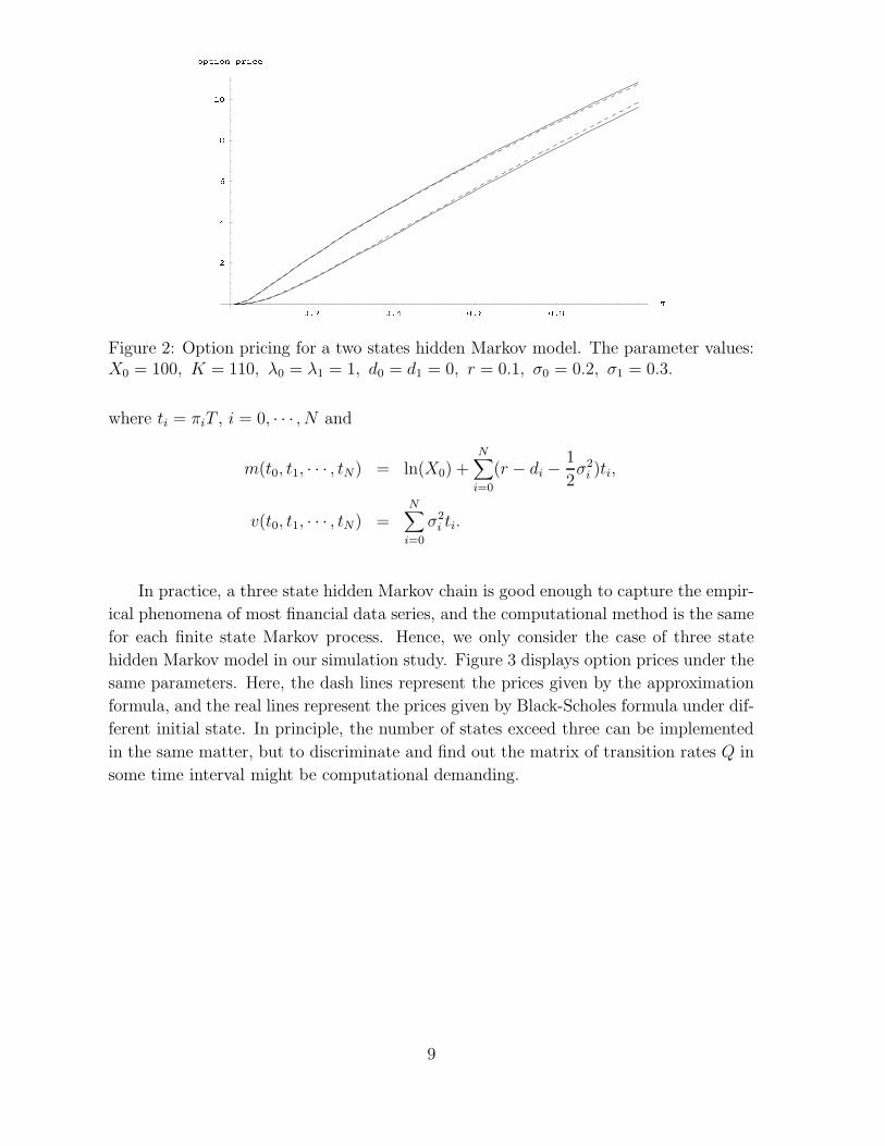
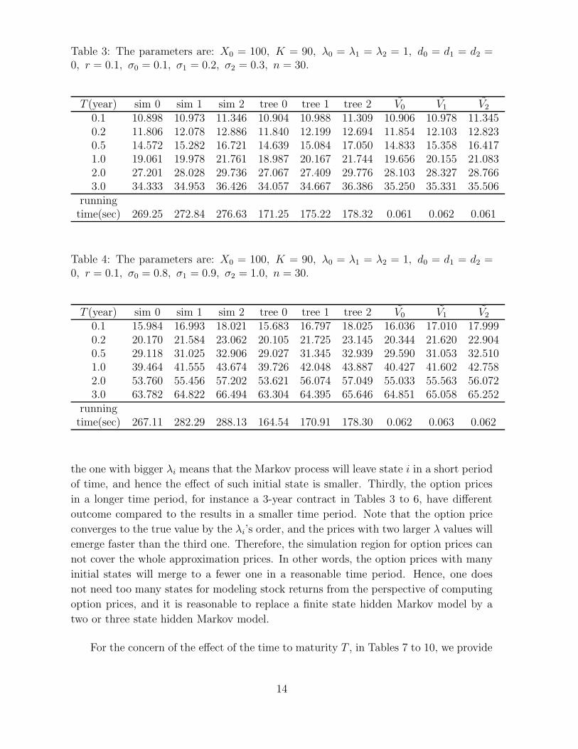
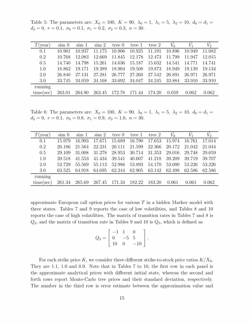
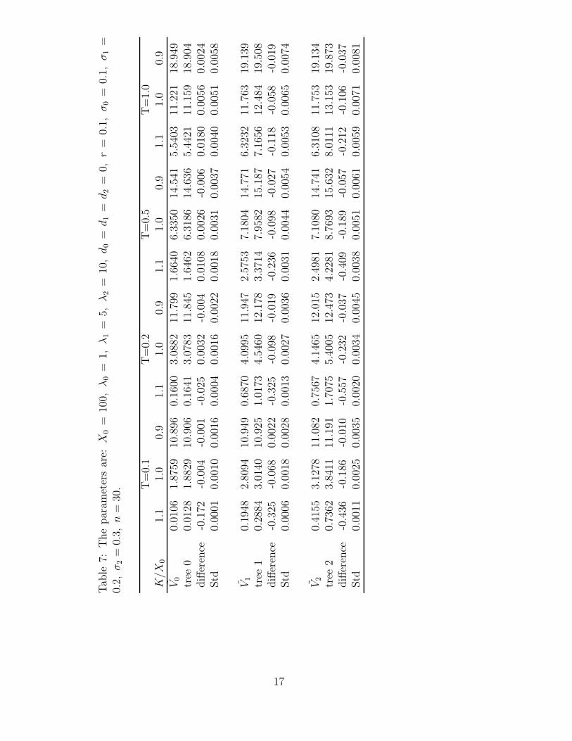
approximate European call option prices for various T in a hidden Markov model with

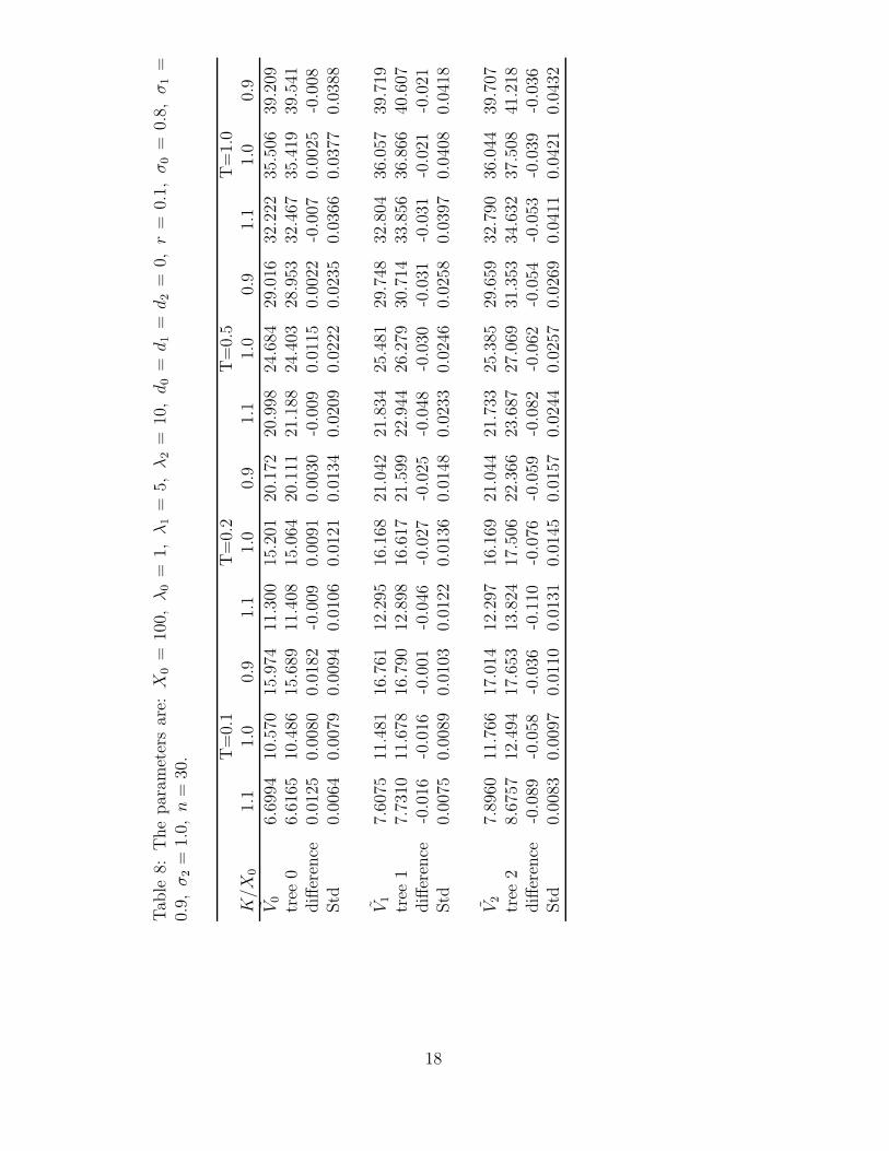
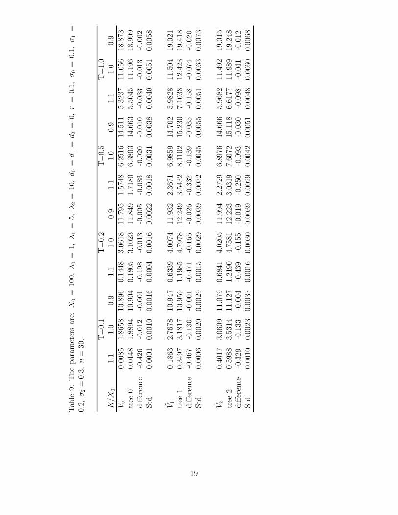
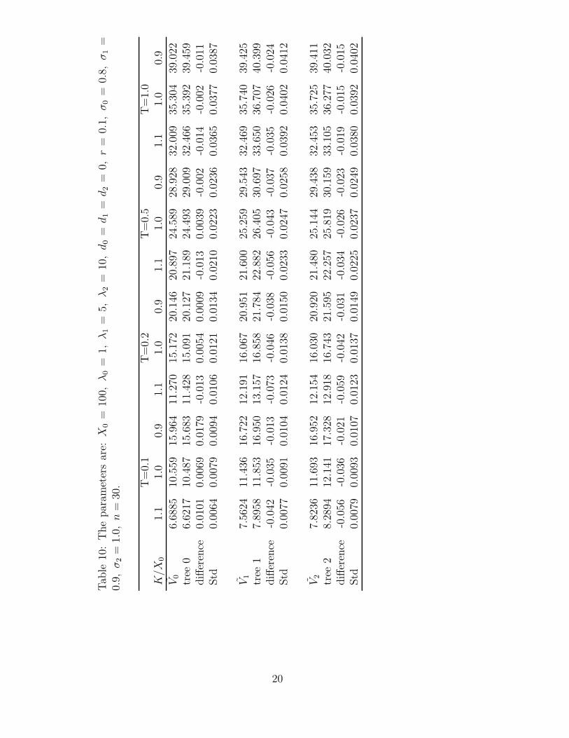
three states. Tables 7 and 9 reports the case of low volatilities, and Tables 8 and 10

reports the case of high volatilities. The matrix of transition rates in Tables 7 and 8 is

Q2, and the matrix of transition rate in Tables 9 and 10 is Q3, which is defined as

Q3 =

−1 1 00 −5 510 0 −10

.

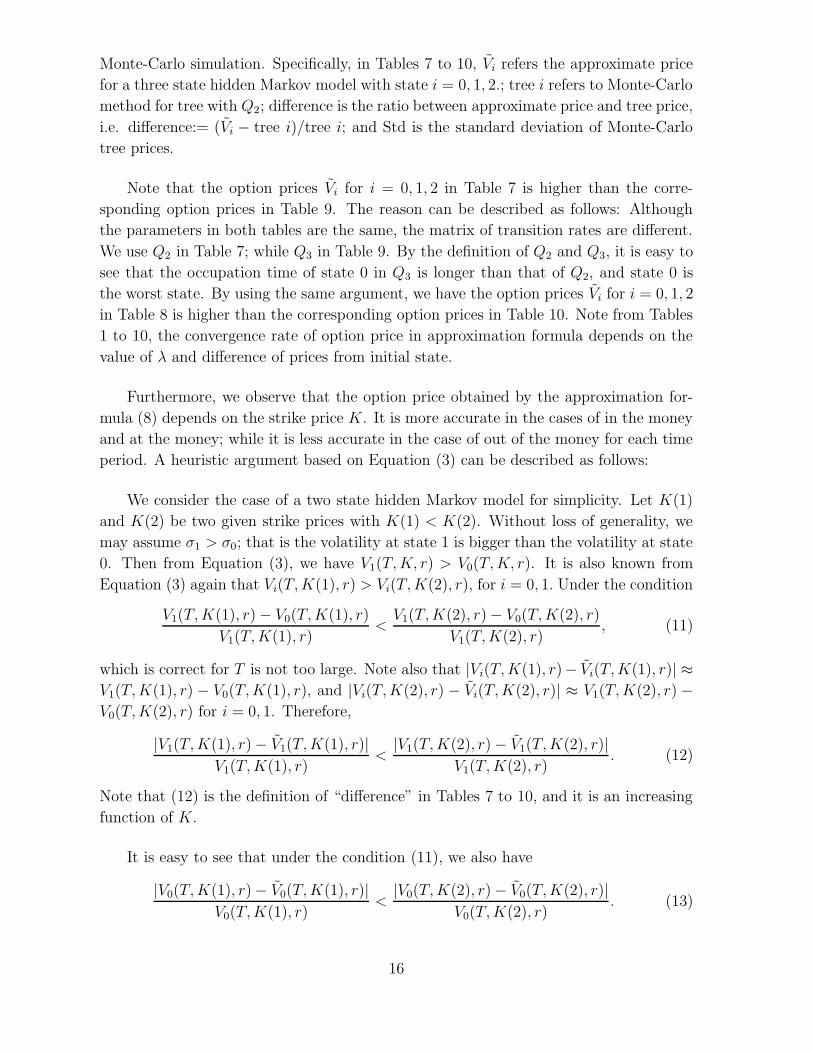
For each strike price K, we consider three different strike-to-stock price ratios K/X0.

They are 1.1, 1.0 and 0.9. Note that in Tables 7 to 10, the first row in each panel is

the approximate analytical prices with different initial state, whereas the second and

forth rows report Monte-Carlo tree prices and their standard deviation, respectively.

The number in the third row is error estimate between the approximation value and

15

Monte-Carlo simulation. Specifically, in Tables 7 to 10, Vi refers the approximate price

for a three state hidden Markov model with state i = 0, 1, 2.; tree i refers to Monte-Carlo

method for tree with Q2; difference is the ratio between approximate price and tree price,

i.e. difference:= (Vi − tree i)/tree i; and Std is the standard deviation of Monte-Carlo

tree prices.

Note that the option prices Vi for i = 0, 1, 2 in Table 7 is higher than the corre-

sponding option prices in Table 9. The reason can be described as follows: Although

the parameters in both tables are the same, the matrix of transition rates are different.

We use Q2 in Table 7; while Q3 in Table 9. By the definition of Q2 and Q3, it is easy to

see that the occupation time of state 0 in Q3 is longer than that of Q2, and state 0 is

the worst state. By using the same argument, we have the option prices Vi for i = 0, 1, 2

in Table 8 is higher than the corresponding option prices in Table 10. Note from Tables

1 to 10, the convergence rate of option price in approximation formula depends on the

value of λ and difference of prices from initial state.

Furthermore, we observe that the option price obtained by the approximation for-

mula (8) depends on the strike price K. It is more accurate in the cases of in the money

and at the money; while it is less accurate in the case of out of the money for each time

period. A heuristic argument based on Equation (3) can be described as follows:

We consider the case of a two state hidden Markov model for simplicity. Let K(1)

and K(2) be two given strike prices with K(1) < K(2). Without loss of generality, we

may assume σ1 > σ0; that is the volatility at state 1 is bigger than the volatility at state

0. Then from Equation (3), we have V1(T,K, r) > V0(T,K, r). It is also known from

Equation (3) again that Vi(T,K(1), r) > Vi(T,K(2), r), for i = 0, 1. Under the condition

V1(T,K(1), r)− V0(T,K(1), r)

V1(T,K(1), r)<V1(T,K(2), r)− V0(T,K(2), r)

V1(T,K(2), r), (11)

which is correct for T is not too large. Note also that |Vi(T,K(1), r)− Vi(T,K(1), r)| ≈V1(T,K(1), r) − V0(T,K(1), r), and |Vi(T,K(2), r) − Vi(T,K(2), r)| ≈ V1(T,K(2), r)−V0(T,K(2), r) for i = 0, 1. Therefore,

|V1(T,K(1), r)− V1(T,K(1), r)|V1(T,K(1), r)

<|V1(T,K(2), r)− V1(T,K(2), r)|

V1(T,K(2), r). (12)

Note that (12) is the definition of “difference” in Tables 7 to 10, and it is an increasing

function of K.

It is easy to see that under the condition (11), we also have

|V0(T,K(1), r)− V0(T,K(1), r)|V0(T,K(1), r)

<|V0(T,K(2), r)− V0(T,K(2), r)|

V0(T,K(2), r). (13)

16

Tab

le7:

The

par

amet

ers

are:

X0

=10

0,λ

0=

1,λ

1=

5,λ

2=

10,d

0=d

1=d

2=

0,r

=0.

1,σ

0=

0.1,

σ1

=0.

2,σ

2=

0.3,n

=30

. T=

0.1

T=

0.2

T=

0.5

T=

1.0

K/X

01.

11.

00.

91.

11.

00.

91.

11.

00.

91.

11.

00.

9

V0

0.01

061.

8759

10.8

960.

1600

3.08

8211

.799

1.66

406.

3350

14.5

415.

5403

11.2

2118

.949

tree

00.

0128

1.88

2910

.906

0.16

413.

0783

11.8

451.

6462

6.31

8614

.636

5.44

2111

.159

18.9

04diff

eren

ce-0

.172

-0.0

04-0

.001

-0.0

250.

0032

-0.0

040.

0108

0.00

26-0

.006

0.01

800.

0056

0.00

24Std

0.00

010.

0010

0.00

160.

0004

0.00

160.

0022

0.00

180.

0031

0.00

370.

0040

0.00

510.

0058

V1

0.19

482.

8094

10.9

490.

6870

4.09

9511

.947

2.57

537.

1804

14.7

716.

3232

11.7

6319

.139

tree

10.

2884

3.01

4010

.925

1.01

734.

5460

12.1

783.

3714

7.95

8215

.187

7.16

5612

.484

19.5

08diff

eren

ce-0

.325

-0.0

680.

0022

-0.3

25-0

.098

-0.0

19-0

.236

-0.0

98-0

.027

-0.1

18-0

.058

-0.0

19Std

0.00

060.

0018

0.00

280.

0013

0.00

270.

0036

0.00

310.

0044

0.00

540.

0053

0.00

650.

0074

V2

0.41

553.

1278

11.0

820.

7567

4.14

6512

.015

2.49

817.

1080

14.7

416.

3108

11.7

5319

.134

tree

20.

7362

3.84

1111

.191

1.70

755.

4005

12.4

734.

2281

8.76

9315

.632

8.01

1113

.153

19.8

73diff

eren

ce-0

.436

-0.1

86-0

.010

-0.5

57-0

.232

-0.0

37-0

.409

-0.1

89-0

.057

-0.2

12-0

.106

-0.0

37Std

0.00

110.

0025

0.00

350.

0020

0.00

340.

0045

0.00

380.

0051

0.00

610.

0059

0.00

710.

0081

17

Tab

le8:

The

par

amet

ers

are:

X0

=10

0,λ

0=

1,λ

1=

5,λ

2=

10,d

0=d

1=d

2=

0,r

=0.

1,σ

0=

0.8,

σ1

=0.

9,σ

2=

1.0,n

=30

. T=

0.1

T=

0.2

T=

0.5

T=

1.0

K/X

01.

11.

00.

91.

11.

00.

91.

11.

00.

91.

11.

00.

9

V0

6.69

9410

.570

15.9

7411

.300

15.2

0120

.172

20.9

9824

.684

29.0

1632

.222

35.5

0639

.209

tree

06.

6165

10.4

8615

.689

11.4

0815

.064

20.1

1121

.188

24.4

0328

.953

32.4

6735

.419

39.5

41diff

eren

ce0.

0125

0.00

800.

0182

-0.0

090.

0091

0.00

30-0

.009

0.01

150.

0022

-0.0

070.

0025

-0.0

08Std

0.00

640.

0079

0.00

940.

0106

0.01

210.

0134

0.02

090.

0222

0.02

350.

0366

0.03

770.

0388

V1

7.60

7511

.481

16.7

6112

.295

16.1

6821

.042

21.8

3425

.481

29.7

4832

.804

36.0

5739

.719

tree

17.

7310

11.6

7816

.790

12.8

9816

.617

21.5

9922

.944

26.2

7930

.714

33.8

5636

.866

40.6

07diff

eren

ce-0

.016

-0.0

16-0

.001

-0.0

46-0

.027

-0.0

25-0

.048

-0.0

30-0

.031

-0.0

31-0

.021

-0.0

21Std

0.00

750.

0089

0.01

030.

0122

0.01

360.

0148

0.02

330.

0246

0.02

580.

0397

0.04

080.

0418

V2

7.89

6011

.766

17.0

1412

.297

16.1

6921

.044

21.7

3325

.385

29.6

5932

.790

36.0

4439

.707

tree

28.

6757

12.4

9417

.653

13.8

2417

.506

22.3

6623

.687

27.0

6931

.353

34.6

3237

.508

41.2

18diff

eren

ce-0

.089

-0.0

58-0

.036

-0.1

10-0

.076

-0.0

59-0

.082

-0.0

62-0

.054

-0.0

53-0

.039

-0.0

36Std

0.00

830.

0097

0.01

100.

0131

0.01

450.

0157

0.02

440.

0257

0.02

690.

0411

0.04

210.

0432

18

Tab

le9:

The

par

amet

ers

are:

X0

=10

0,λ

0=

1,λ

1=

5,λ

2=

10,d

0=d

1=d

2=

0,r

=0.

1,σ

0=

0.1,

σ1

=0.

2,σ

2=

0.3,n

=30

. T=

0.1

T=

0.2

T=

0.5

T=

1.0

K/X

01.

11.

00.

91.

11.

00.

91.

11.

00.

91.

11.

00.

9

V0

0.00

851.

8658

10.8

960.

1448

3.06

1811

.795

1.57

486.

2516

14.5

115.

3237

11.0

5618

.873

tree

00.

0148

1.88

9410

.904

0.18

053.

1023

11.8

491.

7180

6.38

0314

.663

5.50

4511

.196

18.9

09diff

eren

ce-0

.426

-0.0

12-0

.001

-0.1

98-0

.013

-0.0

05-0

.083

-0.0

20-0

.010

-0.0

33-0

.013

-0.0

02Std

0.00

010.

0010

0.00

160.

0004

0.00

160.

0022

0.00

180.

0031

0.00

380.

0040

0.00

510.

0058

V1

0.18

632.

7678

10.9

470.

6339

4.00

7411

.932

2.36

716.

9859

14.7

025.

9828

11.5

0419

.021

tree

10.

3497

3.18

1710

.959

1.19

854.

7978

12.2

493.

5432

8.11

0215

.230

7.10

3812

.423

19.4

18diff

eren

ce-0

.467

-0.1

30-0

.001

-0.4

71-0

.165

-0.0

26-0

.332

-0.1

39-0

.035

-0.1

58-0

.074

-0.0

20Std

0.00

060.

0020

0.00

290.

0015

0.00

290.

0039

0.00

320.

0045

0.00

550.

0051

0.00

630.

0073

V2

0.40

173.

0609

11.0

790.

6841

4.02

0511

.994

2.27

296.

8976

14.6

665.

9682

11.4

9219

.015

tree

20.

5988

3.53

1411

.127

1.21

904.

7581

12.2

233.

0319

7.60

7215

.118

6.61

7711

.989

19.2

48diff

eren

ce-0

.329

-0.1

33-0

.004

-0.4

39-0

.155

-0.0

19-0

.250

-0.0

93-0

.030

-0.0

98-0

.041

-0.0

12Std

0.00

100.

0023

0.00

330.

0016

0.00

300.

0039

0.00

290.

0042

0.00

510.

0048

0.00

600.

0068

19

Tab

le10

:T

he

par

amet

ers

are:X

0=

100,

λ0

=1,

λ1

=5,

λ2

=10,d

0=d

1=d

2=

0,r

=0.

1,σ

0=

0.8,

σ1

=0.

9,σ

2=

1.0,n

=30

. T=

0.1

T=

0.2

T=

0.5

T=

1.0

K/X

01.

11.

00.

91.

11.

00.

91.

11.

00.

91.

11.

00.

9

V0

6.68

8510

.559

15.9

6411

.270

15.1

7220

.146

20.8

9724

.589

28.9

2832

.009

35.3

0439

.022

tree

06.

6217

10.4

8715

.683

11.4

2815

.091

20.1

2721

.189

24.4

9329

.009

32.4

6635

.392

39.4

59diff

eren

ce0.

0101

0.00

690.

0179

-0.0

130.

0054

0.00

09-0

.013

0.00

39-0

.002

-0.0

14-0

.002

-0.0

11Std

0.00

640.

0079

0.00

940.

0106

0.01

210.

0134

0.02

100.

0223

0.02

360.

0365

0.03

770.

0387

V1

7.56

2411

.436

16.7

2212

.191

16.0

6720

.951

21.6

0025

.259

29.5

4332

.469

35.7

4039

.425

tree

17.

8958

11.8

5316

.950

13.1

5716

.858

21.7

8422

.882

26.4

0530

.697

33.6

5036

.707

40.3

99diff

eren

ce-0

.042

-0.0

35-0

.013

-0.0

73-0

.046

-0.0

38-0

.056

-0.0

43-0

.037

-0.0

35-0

.026

-0.0

24Std

0.00

770.

0091

0.01

040.

0124

0.01

380.

0150

0.02

330.

0247

0.02

580.

0392

0.04

020.

0412

V2

7.82

3611

.693

16.9

5212

.154

16.0

3020

.920

21.4

8025

.144

29.4

3832

.453

35.7

2539

.411

tree

28.

2894

12.1

4117

.328

12.9

1816

.743

21.5

9522

.257

25.8

1930

.159

33.1

0536

.277

40.0

32diff

eren

ce-0

.056

-0.0

36-0

.021

-0.0

59-0

.042

-0.0

31-0

.034

-0.0

26-0

.023

-0.0

19-0

.015

-0.0

15Std

0.00

790.

0093

0.01

070.

0123

0.01

370.

0149

0.02

250.

0237

0.02

490.

0380

0.03

920.

0402

20

¿From the results appeared in Tables 3 to 10, we note that the performance of ana-

lytic approximation is very promising, compare to the examined numerically outcomes

obtained by Monte-Carlo simulation and Markovian tree method. The advantage of the

analytical approximation is that it accelerates the computation time of the option prices

in hidden Markov models.

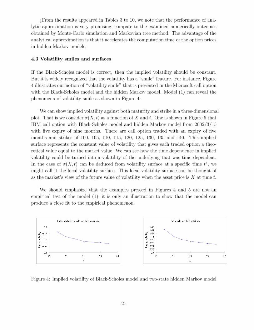
4.3 Volatility smiles and surfaces

If the Black-Scholes model is correct, then the implied volatility should be constant.

But it is widely recognized that the volatility has a “smile” feature. For instance, Figure

4 illustrates our notion of “volatility smile” that is presented in the Microsoft call option

with the Black-Scholes model and the hidden Markov model. Model (1) can reveal the

phenomena of volatility smile as shown in Figure 4.

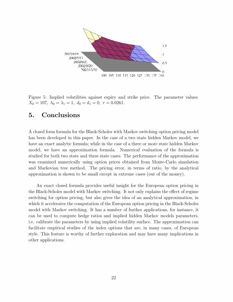
We can show implied volatility against both maturity and strike in a three-dimensional

plot. That is we consider σ(X, t) as a function of X and t. One is shown in Figure 5 that

IBM call option with Black-Scholes model and hidden Markov model from 2002/3/15

with five expiry of nine months. There are call option traded with an expiry of five

months and strikes of 100, 105, 110, 115, 120, 125, 130, 135 and 140. This implied

surface represents the constant value of volatility that gives each traded option a theo-

retical value equal to the market value. We can see how the time dependence in implied

volatility could be turned into a volatility of the underlying that was time dependent.

In the case of σ(X, t) can be deduced from volatility surface at a specific time t∗, we

might call it the local volatility surface. This local volatility surface can be thought of

as the market’s view of the future value of volatility when the asset price is X at time t.

We should emphasize that the examples pressed in Figures 4 and 5 are not an

empirical test of the model (1), it is only an illustration to show that the model can

produce a close fit to the empirical phenomenon.

D=E FGFHI@JLKNM OGPGQ@RSPFGHTE RVUT E HFVQPGT KNW E T E W X

YZ [YZ [G\YZ ]YZ ]\YZ \

]\ \G\ ^G\ _\ `\a

b cdef gh ije klfef l m

no pSqSrsGtuv qVwu v tsVxrGu yNz v u v z

| ~| ~| ~| ~G| ~| | | G|

G

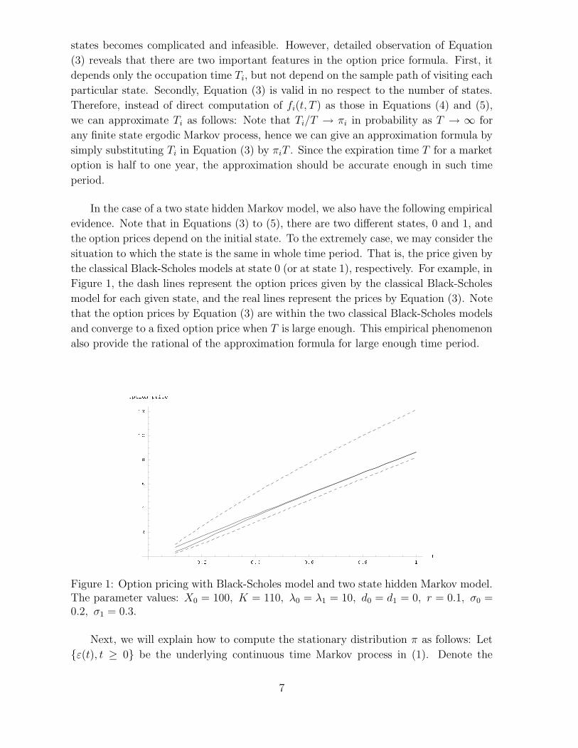
Figure 4: Implied volatility of Black-Scholes model and two-state hidden Markov model

21

-C+ " =

=- == " ==

Figure 5: Implied volatilities against expiry and strike price. The parameter values:X0 = 107, λ0 = λ1 = 1, d0 = d1 = 0, r = 0.0261.

5. Conclusions

A closed form formula for the Black-Scholes with Markov switching option pricing model

has been developed in this paper. In the case of a two state hidden Markov model, we

have an exact analytic formula; while in the case of a three or more state hidden Markov

model, we have an approximation formula. Numerical evaluation of the formula is

studied for both two state and three state cases. The performance of the approximation

was examined numerically using option prices obtained from Monte-Carlo simulation

and Markovian tree method. The pricing error, in terms of ratio, by the analytical

approximation is shown to be small except in extreme cases (out of the money).

An exact closed formula provides useful insight for the European option pricing in

the Black-Scholes model with Markov switching. It not only explains the effect of regime

switching for option pricing, but also gives the idea of an analytical approximation, in

which it accelerates the computation of the European option pricing in the Black-Scholes

model with Markov switching. It has a number of further applications, for instance, it

can be used to compute hedge ratios and implied hidden Markov models parameters,

i.e. calibrate the parameters by using implied volatility surface. The approximation can

facilitate empirical studies of the index options that are, in many cases, of European

style. This feature is worthy of further exploration and may have many implications in

other applications.

22

References

Anderson, T. G. (1996). Return volatility and trading volume: an information

flow interpretation of stochastic volatility. Journal of Finance, 51, 169-204.

Avellaneda, M., Levy, P., and Paras, A. (1995). Pricing and hedging derivative

securities in markets with uncertain volatilities. Applied Mathematical Finance, 2,

73-88.

Bittlingmayer, G. (1998). Output, stock volatility and political uncertainty in a

natural experiment: Germany, 1880-1940. Journal of Finance, 53, 2243-2257.

Black, F. and Scholes, M. (1973). The pricing of options and corporate liabilities.

Journal of Political Economy, 81, 637-654.

Cox, J., Ross, S., and Rubinstein, M. (1979). Option pricing, a simplified approach.

Journal of Financial Economics, 7, 229-263.

David, A. (1997). Fluctuating confidence in stock markets: Implications for re-

turns and volatility. Journal of Financial and Quantitative Analysis, 32, 427-462.

Detemple, J. B. (1991). Further results on asset pricing with incomplete informa-

tion. Journal of Economic Dynamics and Control, 15, 425-453.

Di Masi, G. B., Kabanov, Yu, M., and Runggaldier, W. J. (1994). Mean-variance

hedging of options on stocks with Markov volatility. Theory of Probability and Its

Applications, 39, 173-181.

Diebold, F. X., and Inoue, A. (2001). Long memory and regime switching. Journal

of Econometrics, 105, 131-159.

Duffie, D., and Huang, C. F. (1986). Multiperiod security markets with differential

information. Journal of Mathematical Economics, 15, 283-303.

Follmer, H. and Sondermann, D. (1986). Hedging of nonredundant contingent

claims. In: Hildenbrand and Mas-Colell, eds., Contributions to Mathematical

Economics, 205-223.

Grorud, A., and Pontier, M., (1998). Insider trading in a continuous time market

model. International Journal of Theoretical and Applied Finance, 1, 331-347.

Guilaume, D. M., Dacorogna, M., Dave, R., Muller, U., Olsen, R., and Pictet, P.

(1997). ¿From the bird’s eye to the microscope, a survey of stylized facts of the

intra-daily foreign exchange market. Finance and Stochastics, 1, 95-129.

Guo, X. (2001). Information and option pricing. Journal of Quantitative Finance,

1, 38-44.

23

Hamilton, J. D. (1988). Rational-Expectations econometric analysis of changes in

regime: an investigation of term structure of interest rates. Journal of Economic

Dynamics and Control, 12, 385-423.

Hamilton, J. D. (1989). A new approach to the economic analysis of nonstationary

time series and the business cycle. Econometrica, 57, 357-384.

Hamilton, J. D., and Susmel, R. (1994). Autoregressive conditional heteroscedas-

ticity and changes in regime. Journal of Econometrics, 64, 307-333.

Heston, S. L. (1993). A closed-form solution for options with stochastic volatility

with applications to bond and currency options. Review of Financial Studies, 6,

327-343.

Hull, J. and White, A. (1987). The pricing of options on assets with stochastic

volatility. Journal of Finance, 2, 281-300.

Karatzas, I., and Pikovsky, I. (1996). Anticipative portfolio optimization. Ad-

vances in Applied Probability, 28, 1095-1122.

McKean, H. P. (1969). Stochastic Integrals. Academic Press, New York.

Ross, S. A. (1989). Information and volatility, the no-arbitrage martingale ap-

proach to timing and resolution irrelevancy. Journal of Finance, 44, 1-8.

Schweizer, M. (1991). Option hedging for semimartingales. Stochastic Processes

and their Applications, 37, 339-363.

So, M. K. P., Lam, K., and Li, W. K. (1998). A stochastic volatility model with

Markov switching. Journal of Business & Economic Statistics, 16, 244-253.

Stein, E. M., and Stein, C. J. (1991). Stock prices distribution with stochastic

volatility, an analytic approach. Review of Financial Studies, 4, 727-752.

Turner, C., Startz, R., and Nelson, C. (1989). A Markov model of heteroscendas-

ticity, risk, and learning in the stock market. Journal of Financial Economics, 25,

3-22.

Veronesi, P. (1999). Stock market overreaction to bad news in good times: a

rational expectations equilibrium model. Review of Financial Studies, 12, 5, 975-

1007.

Wiggins, J. B. (1987). Option values under stochastic volatility. Theory and

empirical evidence. Journal of Financial Economics, 19, 351-372.

Appendix

24

Proof of Theorem 1.

Since the arbitrage price of the European option is the discounted expected value of

Xt under the equivalent martingale measure Q, we have

Vi(T,K, r) = EQ[e−rT (XT −K)+|ε(0) = i].

Recalling that

Xt = X0 exp(∫ t

0(r − dε(s) −

1

2σ2

ε(s))ds+∫ t

0σε(s)dW

Qs ),

the key point is to calculate the instantaneous distribution of Xt. Let Yt = lnXt, then

Yt = Y0 +∫ t

0(r − dε(s) −

1

2σ2

ε(s))ds+∫ t

0σε(s)dW

Qs .

Denote Ti as the total time between 0 and T during which ε(t) = 0, starting from

state i, and we consider the probability distribution function fi(t, T ), which is defined

as the probability distribution function of Ti.

Vi(T,K, r) = E[e−rT (XT −K)+|ε(0) = i]= e−rTE[E[(XT −K)+|Ti]|ε(0) = i]= e−rTEi[E[(XT −K)+|Ti]|Fε(0) = i]

= e−rT∫ ∞

0

∫ T

0

y

y +Kρ(ln(y +K), m(t), v(t))fi(t, T )dtdy,

where ρ(x,m(t), v(t)) is the normal density function with expectation m(t) and variance

v(t),

m(t) = ln(X(0)) + (d1 − d0 −1

2(σ2

0 − σ21))t + (r − d1 −

1

2σ2

1)T,

v(t) = (σ20 − σ2

1)t+ σ21T,

and

ρ(x,m(t), v(t)) =1

√

2πv(t)exp(−(x−m(t))2

2v(t)).

Then

fi(t, T )dt = P (∫ T

0χ0(εs)ds ∈ dt),

where χ0 is the indicate function at state 0.

Let

ψi(r, T ) = E[e−r∫ T

0χ0(εs)ds|ε(0) = i]

=∫ ∞

0e−rtfi(t, T )dt

:= Lr(fi(·, T )),

then we haveψi(r, T ) = e−rT e−λiT δ0(i− 0) + e−λiT δ0(1− i)

+∫ T

0e−λiuλiψ1−i(T − u)e−ruδ0(i−0)du.

25

That is,

ψ0(r, T ) = e−rTe−λ0T +∫ T

0e−λ0uλ0ψ1(T − u)e−rudu,

ψ1(r, T ) = e−λ1T +∫ T

0e−λ1uλ1ψ0(T − u)du.

Taking Laplace transforms on both sides, and writing

Ls(ψi(r, ·)) = Ls[Lr(fi(·, T ))(r, ·)]=

∫ ∞

0e−sTψi(r, T )dT

:= ψi(r, s),

then

ψ0(r, s) =1

r + s+ λ0+

λ0

r + s+ λ0ψ1(r, s),

ψ1(r, s) =1

s+ λ1+

λ1

s + λ1ψ0(r, s).

Solving these equations, we get

ψ0(r, s) =s+ λ0 + λ1

s2 + sλ1 + sλ0 + rs+ rλ1,

ψ1(r, s) =r + s+ λ0 + λ1

s2 + sλ1 + sλ0 + rs+ rλ1

.

Taking r the inverse Laplace transform with represent w

L−1r (ψ0(r, s))(w, ·) = e

−sws+ λ0 + λ1

s+ λ1s+ λ0 + λ1

s+ λ1

,

L−1r (ψ1(r, s))(w, ·) = e

−sws+ λ0 + λ1

s+ λ1λ1(s+ λ0 + λ1)

(s+ λ1)2+δ0(w)

s+ λ1.

Again, tacking s the inverse Laplace transform with represent v

L−1s [L−1

r (ψ0(r, s))(w, ·)](·, v) = e−λ0vδ0(v − w) + e−λ1(v−w)−λ0w[λ0I0(2(λ0λ1w(v − w))1/2)

+ (λ0λ1w

v − w)1/2I1(2(λ0λ1w(v − w))1/2)],

L−1s [L−1

r (ψ1(r, s))(w, ·)](·, v) = e−λ1vδ0(v − w) + e−λ1(v−w)−λ0w[λ1I0(2(λ0λ1w(v − w))1/2)

+ (λ1λ0(v − w)

w)1/2I1(2(λ0λ1w(v − w))1/2)].

Thus, we get f0(w, v) and f1(w, v), the distribution function of T0 and T1, such that

f0(w, v) = e−λ0vδ0(v − w) + e−λ1(v−w)−λ0w[λ0I0(2(λ0λ1w(v − w))1/2)

+ (λ0λ1w

v − w)1/2I1(2(λ0λ1w(v − w))1/2)],

f1(w, v) = e−λ1vδ0(v − w) + e−λ1(v−w)−λ0w[λ1I0(2(λ0λ1w(v − w))1/2)

+ (λ1λ0(v − w)

w)1/2I1(2(λ0λ1w(v − w))1/2)].

26