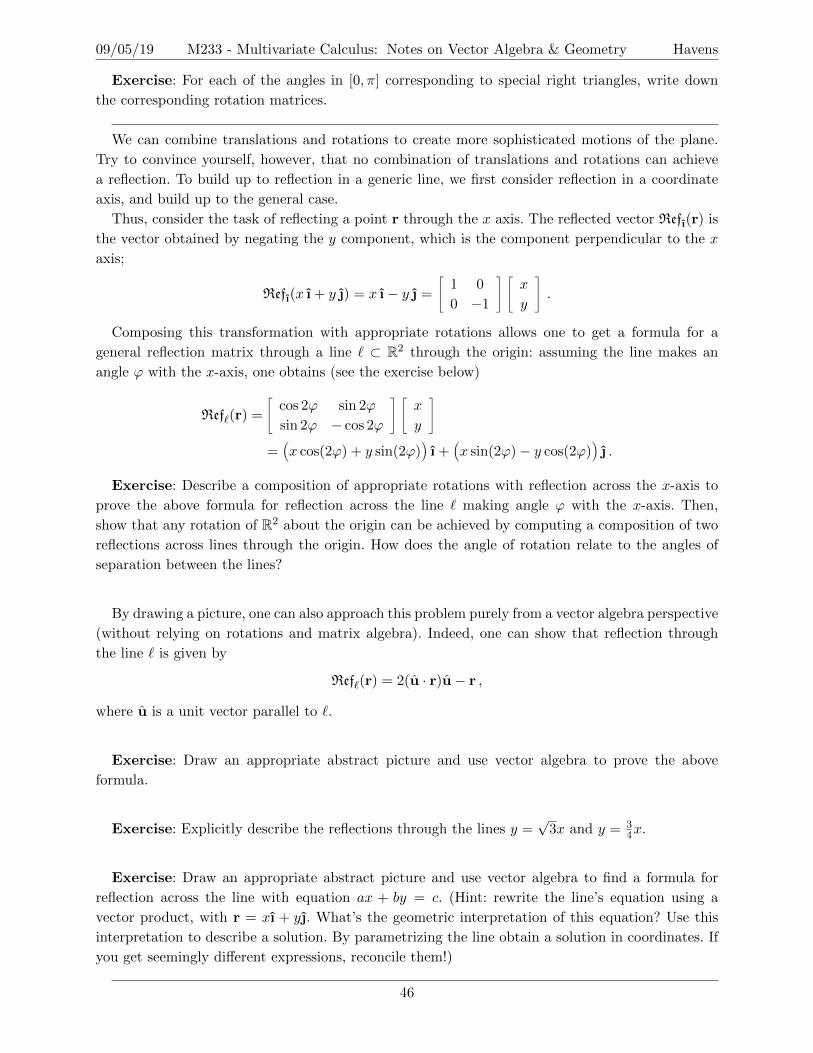
Page 1
VECTOR ALGEBRA
A. HAVENS
Vectors in the context of physics, engineering, and other sciences are mathematical objects rep-
resenting phenomena in space that possess two attributes: direction, and magnitude.
They are the natural geometric objects for describing instantaneous linear motion or action, such
as displacements, velocities, forces, and, once given an origin (a distinguished point in space), posi-
tion. Thus, we will encounter position vectors, displacement vectors, velocities, forces and more, all
collectively obeying algebraic rules that capture their geometric behaviors. Employing coordinates,
we can give vectors a concrete life with which computations can be performed; we will nevertheless
prefer geometric and coordinate-free definitions first in these notes, and derive the relevant coordi-
nate rules from our geometric intuition whenever possible. Occasionally this kind of thinking will
be relegated to the exercises and problems at the end of each section.
There is an optional section at the end which explores the mathematics behind certain geometric
transformations of two and three dimensional space, and connects these to the history of vectors,
via Hamilton’s theory of quaternions.
Contents
1 Vectors and Coordinates 1
1.1 Defining vectors geometrically . . . . . . . . . . . . . . . . . . . . . . . . . . . . 1
1.2 Addition, Subtraction, and Scaling . . . . . . . . . . . . . . . . . . . . . . . . . . 2
1.3 Vectors in Coordinates . . . . . . . . . . . . . . . . . . . . . . . . . . . . . . . . 4
1.4 Problems . . . . . . . . . . . . . . . . . . . . . . . . . . . . . . . . . . . . . . . . 11
2 The Dot Product 13
2.1 Motivation from Projections . . . . . . . . . . . . . . . . . . . . . . . . . . . . . 13
2.2 Coordinate Expressions . . . . . . . . . . . . . . . . . . . . . . . . . . . . . . . . 15
2.3 Algebraic Properties . . . . . . . . . . . . . . . . . . . . . . . . . . . . . . . . . . 16
2.4 Simple applications of the dot product . . . . . . . . . . . . . . . . . . . . . . . . 16
2.5 Problems . . . . . . . . . . . . . . . . . . . . . . . . . . . . . . . . . . . . . . . . 21
3 Cross Product 25
3.1 Geometric Definition . . . . . . . . . . . . . . . . . . . . . . . . . . . . . . . . . . 25
3.2 Physical Definition . . . . . . . . . . . . . . . . . . . . . . . . . . . . . . . . . . . 25
3.3 Algebraic and Geometric properties . . . . . . . . . . . . . . . . . . . . . . . . . 27
3.4 Deriving Coordinate Expressions . . . . . . . . . . . . . . . . . . . . . . . . . . . 27
3.5 Determinants and Areas . . . . . . . . . . . . . . . . . . . . . . . . . . . . . . . . 29
3.6 Triple Products . . . . . . . . . . . . . . . . . . . . . . . . . . . . . . . . . . . . 30
3.7 Problems . . . . . . . . . . . . . . . . . . . . . . . . . . . . . . . . . . . . . . . . 33
4 Lines 36
4.1 Vector Equations and Parametric Equations . . . . . . . . . . . . . . . . . . . . 36
4.2 Symmetric Equations . . . . . . . . . . . . . . . . . . . . . . . . . . . . . . . . . 38i
Page 2
09/05/19 M233 - Multivariate Calculus: Notes on Vector Algebra & Geometry Havens
4.3 Problems . . . . . . . . . . . . . . . . . . . . . . . . . . . . . . . . . . . . . . . . 38
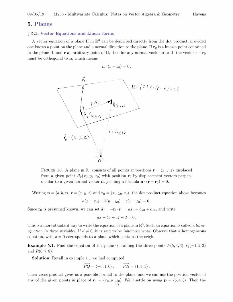
5 Planes 40
5.1 Vector Equations and Linear forms . . . . . . . . . . . . . . . . . . . . . . . . . . 40
5.2 Distances . . . . . . . . . . . . . . . . . . . . . . . . . . . . . . . . . . . . . . . . 42
5.3 Problems . . . . . . . . . . . . . . . . . . . . . . . . . . . . . . . . . . . . . . . . 43
6 Geometry of rigid motions in the plane and 3-Space* 45
6.1 Translations, Rotations, and Reflections in the plane . . . . . . . . . . . . . . . . 45
6.2 Complex multiplication and planar geometry . . . . . . . . . . . . . . . . . . . . 47
6.3 Spatial motions via vector algebra . . . . . . . . . . . . . . . . . . . . . . . . . . 49
6.4 Quaternions . . . . . . . . . . . . . . . . . . . . . . . . . . . . . . . . . . . . . . 49
6.5 Problems . . . . . . . . . . . . . . . . . . . . . . . . . . . . . . . . . . . . . . . . 52
ii
Page 3
09/05/19 M233 - Multivariate Calculus: Notes on Vector Algebra & Geometry Havens
1. Vectors and Coordinates
We will give an informal definition of geometric vectors in dimensions ≤ 3, and begin to introduce
the notations common for working with them, in particular in three dimensions. Thus, this section
presumes familiarity with 3-dimensional rectangular coordinates. Later in the course we will see
other coordinate systems (such as polar coordinates), which we will define as needed. We will not
formally define vector spaces, deferring such treatment to a linear algebra course.
We’ll label vectors by bolded letters, as distinguished from real (or complex numbers), which
are written in italics. As our definitions of vectors as well as the algebra we will do with them are
presently grounded in real numbers, it is important to be fluent in real arithmetic and algebra.
The set of all reals will be denoted R, while the real plane will be denoted R2 := R × R, and real
3-dimensional space will be denoted by R3 := R × R × R. We will refer to the reals as scalars, in
keeping with standard language to distinguish the base field from the spaces of vectors built in real
coordinates.
§ 1.1. Defining vectors geometrically
In practice, we wish to model vectors as arrows with a definite direction and length, sitting in
our favorite (real, Euclidean) space, such as the plane R2 or 3-dimensional space R3. By direction,
we mean two things: the arrow determines a line segment, and this line segment has an orientation.
When we draw this, the arrow’s head will tell us the orientation. More formally, we can describe a
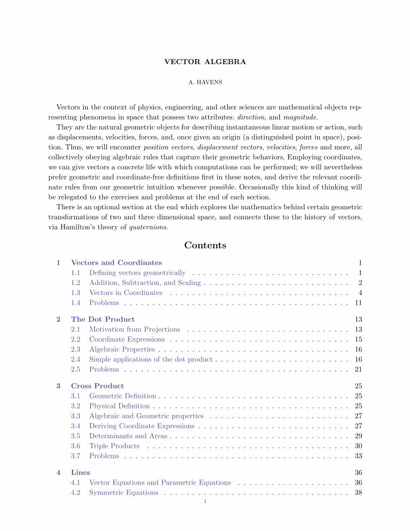
vector’s anatomy as follows: there is an initial point in space, sometimes referred to as the tail, and
a terminal point, often called the tip. The direction is then determined by the oriented line segment
going from this initial point to the terminal point. See figure (1a). The initial and terminal points
may coincide, in which case we have a distinguished case, to be discussed momentarily when we
begin to define vector arithmetic.
(a) (b)
Figure 1. (a) – Anatomy of a vector. (b) – Various equivalent vectors.
We’ll call two vectors parallel if their corresponding line segments are parallel, even if the ori-
entations do not match. But for two vectors to have the same direction, we require that the line
segments be parallel, and that the orientations match. Equivalently, two vectors have the same
direction if and only if there is a continuous motion through similarity transformations taking one
arrow to the other through parallel arrows, i.e. via translation and dilation, but without rotation
or reflection.
We’ll assume the usual means of measurement in space, and thus there is a length, given by
a non-negative real number, associated to the line segments. The magnitude of a vector is this1
Page 4
09/05/19 M233 - Multivariate Calculus: Notes on Vector Algebra & Geometry Havens
length, and for a vector v the magnitude is denoted ‖v‖, or sometimes simply |v|. Some texts use
the convention that the italic letter denotes the magnitude of the corresponding boldfaced vector,
e.g. ‘v’ denotes ‖v‖, however we will prefer clarity and write the double-bar magnitude notation
with few exceptions1.
We will often say two vectors u,v are equivalent if and only if their directions are the same
and their magnitudes equal, and we will write u = v; see figure (1b). Observe that two vectors
u,v with different initial points are equivalent if and only if the translation taking the initial point
of u to the initial point of v translates the terminal point of u to the terminal point of v. Be
aware that in applications we may have cause to prefer to place a vector with a particular initial or
terminal point, but there is no preferred location for our abstract vectors in the sense of the above
equivalence.
We remark that is convenient to define things like “the space of all real, 3-dimensional vectors”.
To do so rigorously, we would need to explore vector spaces and linear algebra in greater detail, but
nevertheless it is convenient to have a notation for such things. Let V 3R be the set of all 3-dimensional
vectors, up to the defined equivalence, and similarly let V 2R be the set of all 2-dimensional vectors
up to the defined equivalence. Even more generally, there are higher dimensional analogs, here
denoted V nR , which are sets of n-vectors. All these sets will have additional structure coming from
the algebra of vectors we will define, making them into vector spaces2, but the abstract study of
vector space structure is the concern of a linear algebra course; we will but glimpse at it and focus
on the calculations and their applications as are pertinent to our study of multivariate calculus.
Thus, even if V nR is written, you may imagine for ease of use that n = 2 or 3, and picture the
comfortable world of arrows drawn on blackboards.
§ 1.2. Addition, Subtraction, and Scaling
Our geometric description of vectors as arrows, pointing from an initial point to a terminal
point, allows us to give pictorial definitions for many of the concepts we will be concerned with.
But to actually manipulate and compute with vectors, it is desirable to have representations that
take advantage of coordinate systems. Before we do this though, we will introduce a notion of
vector arithmetic. Vectors are useful precisely because they allow us to model linear motion and
displacement: unlike points, which are static and admit no inherent arithmetic, vectors may be
added and subtracted to describe changes in position, rates or directions of travel or acceleration,
rotations in 3-space, and many other phenomena.
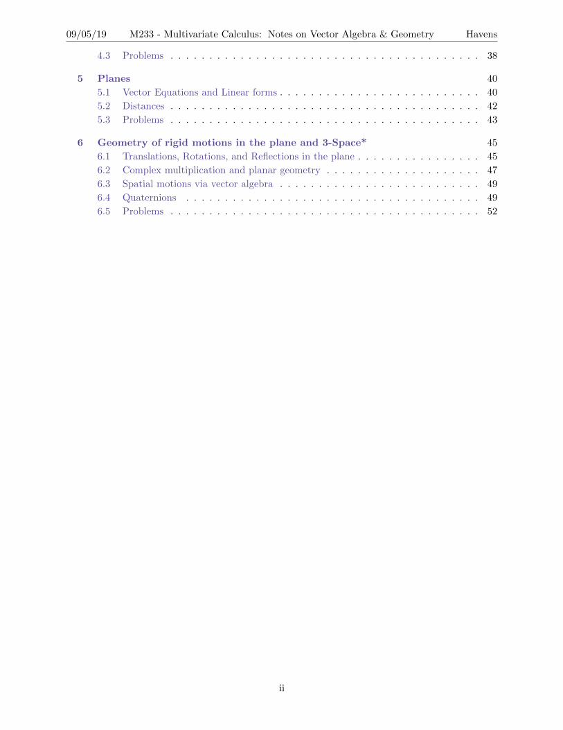
The initial and essential idea is that by placing vectors tail to tip, we locate a new terminal point
and may construct a new vector from the initial point of the first vector to the terminal point of
the last vector of the sum. The result of vector summation is sometimes called the resultant.
Consider the parallelogram in figure (2a), depicting the pair of vectors u and v emanating from a
common initial point, their translates which we label as u and v as well, (in keeping with our notion
of equivalence given above), and their sum, which is the diagonal vector of the parallelogram. The
figure illustrates the so called parallelogram rule of vector addition.
We can derive a subtraction rule from this picture by relabeling the figure and reversing the
orientation of u. Denote by w the vector u + v, and by −u the vector obtained by reversing the
1In physical applications and in the context of polar coordinates, it is convenient sometimes to use a convention
similar to the “bold denotes vectors, italic denotes scalar magnitudes of corresponding vectors.” In such cases, symbols
will be clearly defined in reference to the notations used throughout.2If you want to learn about the zoo of other vector spaces with which mathematicians fascinate themselves, I
highly recommend you take some linear algebra, or come bug me to motivate its study.
2
Page 5
09/05/19 M233 - Multivariate Calculus: Notes on Vector Algebra & Geometry Havens
(a)(b)
Figure 2. (a) – the parallelogram rule. (b) – the vector subtraction triangle rule.
direction of . It is then clear from the preceding definitions that w + −u = v. Thus, adding the
reverse of u to w recovers v. We then may define vector subtraction to be the operation of adding
the reverse, and we will simply write w−u instead of w +−u. Observe that subtraction satisfies a
diagrammatic rule of“closing a triangle”: if w and u are vectors emanating from a common initial
point, then w− u is the vector closing the triangle so that if its initial point is placed at the tip of
u, its terminal point will coincide with the terminal point of w, i.e. it completes the triangle and
points from u to w.
An issue remains: if vectors can be added and the addition is invertible via subtraction, there
ought to be an identity element! Indeed, the vector whose initial and terminal points coincide gives
us such an identity. We call this vector the zero vector, and denote it by 0. The zero vector is the
unique directionless vector and the unique vector of length zero. It is conventionally considered
both parallel and perpendicular to all other vectors (a caveat we will address and exploit later).
The zero vector satisfies v + 0 = v and v − v = 0, where v is any vector.
One may certainly consider iterated addition as one does for integers and real numbers. It is
natural to write for an integer n
nv = v + . . .+ v︸ ︷︷ ︸n times
=n∑i=1
v .
This has an obvious geometric interpretation: nv is the result of stretching v by a factor of n, that
is, the magnitude of nv is n times that of v. There is however no need to restrict ourselves to only
integer stretching. For any positive real number s, the vector sv is the vector whose direction is
the same as v and whose length is s ‖v‖. For a negative real number s, we take sv to denote the
vector whose direction is the same as the reverse of v, and whose length is |s| ‖v‖, i.e., sv = −|s|vfor negative s. Naturally, for s = 0 or for v = 0, we can take sv = 0.
Proposition. The following properties hold for any vectors u,v,w in V nR and any scalars s, t ∈ R.
(1) u + 0 = u (vector additive identity)
(2) 1u = u (scaling identity)
(3) u + (−1)u = u +−u = 0 (vector additive inverse)
(4) u + v = v + u (commutativity of vector addition)
(5) (u + v) + w = u + (v + w) (associativity of vector addition)
(6) s(u + v) = su + sv (distributivity of scaling)
(7) su + tu = (s+ t)u (factoring of scalars)
(8) (st)u = s(tu) (associativity of scaling)3
Page 6
09/05/19 M233 - Multivariate Calculus: Notes on Vector Algebra & Geometry Havens
Figure 3. Scaling a vector.
(9) 0v = 0 (annihilation by zero scaling)
(10) ‖u‖ ≥ 0, with equality ⇐⇒ u = 0 (non-degeneracy of magnitude)
(11) ‖u + v‖ ≤ ‖u‖+ ‖v‖ (triangle inequality for magnitudes)
(12) ‖sv‖ = |s| ‖v‖ (absolute scalability of magnitude)
A good exercise is to verify that the three dimensional vectors we have described satisfy each of
the above properties, using only the geometric definitions given for vector addition and scaling, and
known properties of real numbers. The first eight statements are the axioms of an abstract vector
space with real scalars, while the last three make V nR into a normed vector space. Property (9) is a
simple consequence of preceding properties.
§ 1.3. Vectors in Coordinates
We start by describing position vectors, i.e. vectors describing the positions of points in space.
Consider first a point P (x1, y1, z1) ∈ R3. Then the position vector p associated to P is the vector
whose initial point is the origin (0, 0, 0) ∈ R3 and whose terminal point is P . This motivates the
following coordinate description of p: we write
p = 〈x1, y1, z1〉 .
This notation is referred to as angle bracket notation. The angle bracket notation, while convenient,
somewhat obscures the relation between the coordinates and vector addition. To see this relationship
more concretely, we need another notation.
We define three special coordinate vectors, whose labels are historical3:
ı := 〈1, 0, 0〉 , := 〈0, 1, 0〉 , k := 〈0, 0, 1〉 .
Note that these give the position vectors for points a unit distance from the origin along the positive
coordinate axes. Using the definition of vector addition, it is clear (see the figure below) that
p = x1ı + y1 + z1k .
The numbers x1, y1, and z1 are called the components in the ı, , and k directions, respectively. It
is not uncommon to also refer to them respectively as the x, y and z components. An expression of
the form au1 + bu2 + cu3 for scalars a, b, c ∈ R and vectors u1, u2, u3 is called a linear combination
of the vectors u1, u2, and u3; thus writing the coordinate form of p amounts to expressing it as a
linear combination of the coordinate vectors ı, and k.4
Page 7
09/05/19 M233 - Multivariate Calculus: Notes on Vector Algebra & Geometry Havens
Figure 4. Visualizing the components of a vector in three dimensions.
A further notation, common in linear algebra, is to write the components vertically in a column
enclosed in a bracket or parentheses as follows:
p =
x1
y1
z1
or p =
Öx1
y1
z1
è.
This notation is convenient when describing linear algebraic operations, such as matrix multiplica-
tion, acting on vectors. We will use this notation sparingly in these notes.
For each of the above notations, one may omit the third component (i.e. the z1k term) and
obtain a notation suited to describing two-dimensional vectors. The convention of writing elements
of V 2R in coordinates as linear combinations of ı and conveniently also gives us a natural way to
view the vector space V 2R as being embedded in V 3
R , just as the xy-coordinate plane sits in R3. If
we need to strongly emphasize the difference between a planar vector xı + y and a spatial vector
with the same coordinates, we will write the latter as xı + y + 0k, or in angle bracket notation
〈x, y, 0〉.
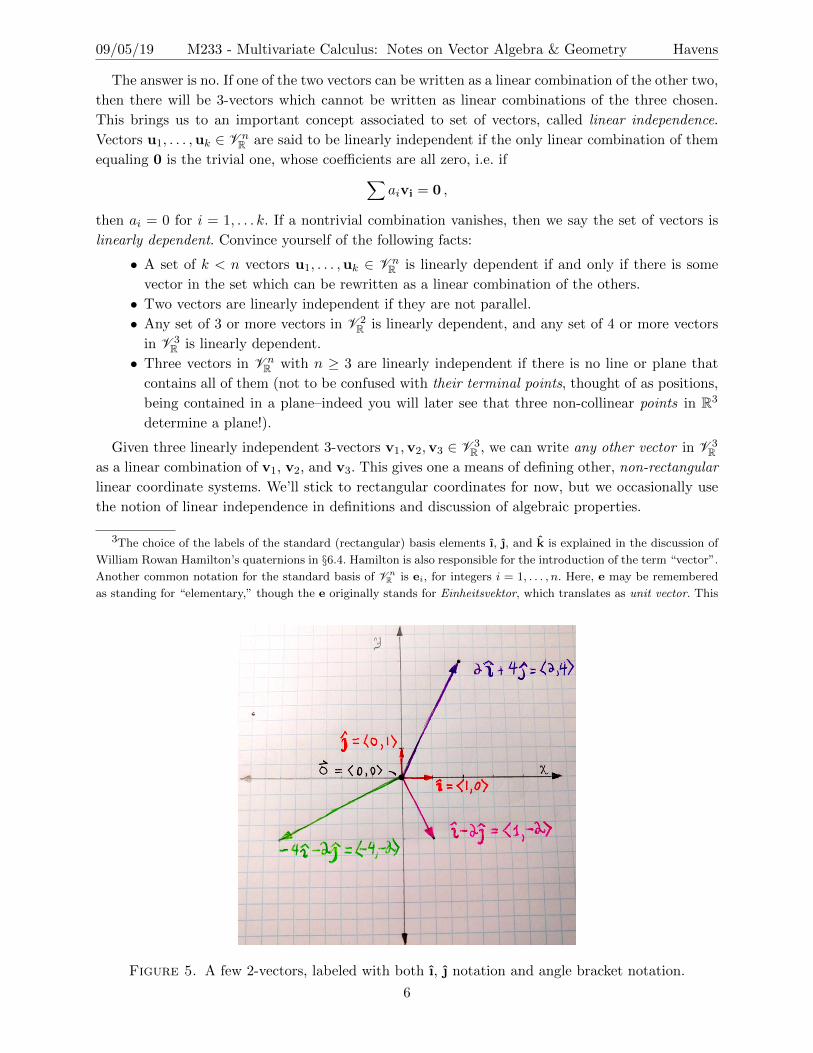
Example 1.1. Figure 5 illustrates several position 2-vectors with accompanying coordinate repre-
sentations. Note that for R2 we define ı = 〈1, 0〉 and = 〈0, 1〉.
An arbitrary vector has a coordinate expression which can be found by translating the initial
point to the origin, and treating it as a position vector, thus any v ∈ V 3R can be described in
coordinates using angle bracket notation, as a linear combination of the vectors ı, , and k, or
in column notation. Each coordinate notation involves listing the same triple of numbers, just in
a slightly different fashion. We can thus easily interpret the components as representing weights
in a linear combination, building the vector v by specifying vectors parallel to the rectangular
coordinate axes.
Many students first encounter the idea of components in physics, where vectors representing
physical data such as velocities or forces are often decomposed as sums of vectors along directions
chosen sensibly for a given physical configuration. This is not so different from our components: the
essential idea of components is just to decompose vectors as linear combinations of some chosen set
of vectors, and in our case we chose the (seemingly natural) set of vectors ı, , and k as a basis to
build other vectors. But can one just choose any three vectors to build all of V 3R ?
5
Page 8
09/05/19 M233 - Multivariate Calculus: Notes on Vector Algebra & Geometry Havens
The answer is no. If one of the two vectors can be written as a linear combination of the other two,
then there will be 3-vectors which cannot be written as linear combinations of the three chosen.
This brings us to an important concept associated to set of vectors, called linear independence.
Vectors u1, . . . ,uk ∈ V nR are said to be linearly independent if the only linear combination of them
equaling 0 is the trivial one, whose coefficients are all zero, i.e. if∑aivi = 0 ,
then ai = 0 for i = 1, . . . k. If a nontrivial combination vanishes, then we say the set of vectors is
linearly dependent. Convince yourself of the following facts:
• A set of k < n vectors u1, . . . ,uk ∈ V nR is linearly dependent if and only if there is some
vector in the set which can be rewritten as a linear combination of the others.
• Two vectors are linearly independent if they are not parallel.
• Any set of 3 or more vectors in V 2R is linearly dependent, and any set of 4 or more vectors
in V 3R is linearly dependent.
• Three vectors in V nR with n ≥ 3 are linearly independent if there is no line or plane that
contains all of them (not to be confused with their terminal points, thought of as positions,
being contained in a plane–indeed you will later see that three non-collinear points in R3
determine a plane!).
Given three linearly independent 3-vectors v1,v2,v3 ∈ V 3R , we can write any other vector in V 3
Ras a linear combination of v1, v2, and v3. This gives one a means of defining other, non-rectangular
linear coordinate systems. We’ll stick to rectangular coordinates for now, but we occasionally use
the notion of linear independence in definitions and discussion of algebraic properties.
3The choice of the labels of the standard (rectangular) basis elements ı, , and k is explained in the discussion of
William Rowan Hamilton’s quaternions in §6.4. Hamilton is also responsible for the introduction of the term “vector”.
Another common notation for the standard basis of V nR is ei, for integers i = 1, . . . , n. Here, e may be remembered
as standing for “elementary,” though the e originally stands for Einheitsvektor, which translates as unit vector. This
Figure 5. A few 2-vectors, labeled with both ı, notation and angle bracket notation.
6
Page 9
09/05/19 M233 - Multivariate Calculus: Notes on Vector Algebra & Geometry Havens
An arbitrary vector drawn with initial point P (x1, y1, z1) and terminal point Q(x2, y2, z2) can
be regarded as a displacement vectorÐÐ⇀PQ, modeling how Q is displaced from P . Since we wish to
express such vectors in coordinates, we need to understand coordinate arithmetic.
Let a = a1ı + a2k and b = b1ı + b2 be two arbitrary position vectors in the plane. From figure
(6) and the known properties of vector arithmetic, it should be clear that the coordinate forms for
vector addition and scaling are given as
a + b = (a1 + b1)ı + (a2 + b2) = 〈a1 + b1, a2 + b2〉 ,
sa = sa1ı + sa2 = 〈sa1, sa2〉 .
We can easily generalize this to 3-vectors, to deduce that vector addition is performed by adding
like components, and scaling a vector by a scalar s scales each component by s individually.
Figure 6. Adding 2-vectors by adding their components. Can you draw a pictorial
proof for 3-vectors? What algebraic properties from above would you use to prove
the analogous result at once for n-vectors with arbitrary n ≥ 3?
Returning to the issue of representing displacement vectors in coordinates, it becomes clear (draw
a picture!) that we can represent the displacement vectorÐÐ⇀PQ as the vector difference q− p of the
corresponding position vectors for the terminal and initial points. Thus, if p = x1ı + y1 + z1k and
q = x2ı + y2 + z2k then
ÐÐ⇀PQ = q− p = (x2 − x1)ı + (y2 − y1) + (z2 − z1)k .
Example 1.2. The points Q(−1, 5, 3) and R(6, 7, 8) are vertices of a parallelogram adjacent to a
vertex at P (5, 4, 3). Find the fourth vertex.
Solution: Since Q and R are each adjacent to P , the displacement vectorsÐÐ⇀PQ and
ÐÐ⇀PR represent
sides of the parallelogram. Let S denote the fourth point of the parallelogram. By applying the
parallelogram rule, we can find a displacement vectorÐ⇀PS from P to the fourth point. Namely,
Ð⇀PS =
ÐÐ⇀PQ+
ÐÐ⇀PR .
In coordinates, we have
ÐÐ⇀PQ = q− p = 〈−6, 1, 0〉 ,
ÐÐ⇀PR = r− p = 〈1, 3, 5〉 .
notation was introduced by Hermann Grassmann, in his seminal work Die Lineale Ausdehnungslehre, ein neuer Zweig
der Mathematik published in 1844.
7
Page 10
09/05/19 M233 - Multivariate Calculus: Notes on Vector Algebra & Geometry Havens
ThusÐ⇀PS = 〈−6, 1, 0〉+ 〈1, 3, 5〉 = 〈−5, 4, 5〉 .
The coordinates of S can be found by adding the position vector p for P to the displacement vectorÐ⇀PS, since P is the initial point of the displacement vector, and the desired point S is the terminal
point. Thus, the position vector s for the point S is
s = p +Ð⇀PS = 〈5, 4, 3〉+ 〈−5, 4, 5〉 = 〈0, 8, 8〉 .
This gives the fourth point as S(0, 8, 8). In general, to solve a problem like this, one may note that
Ð⇀PS = q− p + r− p and
Ð⇀PS = s− p , whence
s− p = q− p + r− p =⇒ s = q + r− p .
One can now check that, indeed,
〈0, 8, 8〉 = 〈−1, 5, 3〉+ 〈6, 7, 8〉 − 〈5, 4, 3〉 .
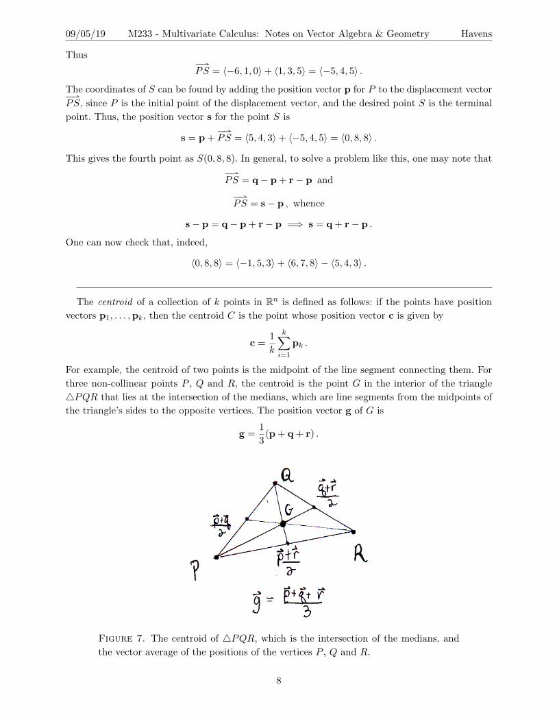
The centroid of a collection of k points in Rn is defined as follows: if the points have position
vectors p1, . . . ,pk, then the centroid C is the point whose position vector c is given by
c =1
k
k∑i=1
pk .
For example, the centroid of two points is the midpoint of the line segment connecting them. For
three non-collinear points P , Q and R, the centroid is the point G in the interior of the triangle
4PQR that lies at the intersection of the medians, which are line segments from the midpoints of
the triangle’s sides to the opposite vertices. The position vector g of G is
g =1
3(p + q + r) .
Figure 7. The centroid of 4PQR, which is the intersection of the medians, and
the vector average of the positions of the vertices P , Q and R.
8
Page 11
09/05/19 M233 - Multivariate Calculus: Notes on Vector Algebra & Geometry Havens
Example 1.3. Find the centroid of the points P (π, e), Q(1/e,−π), and R(√π, eπ).
Solution: The position vectors are
p = πı + e , q = 1/eı− π , r =√πı + eπ .
Thus the centroid has position vector
g =1
3
Äπı + e + 1/eı− π +
√πı + eπ
ä=
1
3(π + 1/e+
√π)ı +
1
3(e− π + eπ ) .
Thus
G
Çπ + 1/e+
√π
3,e− π + eπ
3
åis the centroid of 4PQR.
Using the Pythagorean theorem, one can readily confirm that our notion of vector magnitude
should be computable by summing the squares of components, and then taking the square root of
this sum. Thus if a = a1ı + a2 + a3k, we have
‖a‖ =»a2
1 + a22 + a2
3 .
A vector is called a unit vector if it has length 1. To get a unit vector from another vector, we
scale by the reciprocal of the magnitude:
u 7→ u =u
‖u‖.
Here, the hat ‘ ’ in u denotes that it is a unit vector. Conventionally, if you see a vector with a hat
in these notes, it has length 1.
Example 1.4. Find a unit vector in the direction of 3ı + 4, and a unit vector making an angle of
π/3 with ı.
Solution: The magnitude of 3ı + 4 is√
32 + 42 =√
25 = 5, so the unit vector in the same
direction as 3ı + 4 is 35 ı + 4
5 . For a unit vector making an angle of π/3 with ı, we can draw a right
triangle based at the origin, parallel to ı, with length one hypotenuse. Then the desired unit vector
has initial point at the origin and final point with coordinates (cos π3 , sinπ3 ) = (1
2 ,√
32 ), whence the
desired unit vector is 12 ı +
√3
2 .
Example 1.5. Resolve the vector v with magnitude 2 making an angle of π/12 with the positive
x-axis into x and y components.
Solution: A vector v making an angle θ with the positive x-axis determines an arrow the line
segment of which, when placed with its tail at the origin, forms the hypotenuse of a right triangle
with a horizontal leg of length ‖v‖ cos θ and a vertical leg of length ‖v‖ sin θ. For our example, v
has ‖v‖ = 2 and θ = π/12, so it resolves into components as
v = 2 cos( π
12
)ı + 2 sin
( π12
) =
⟨2 cos
( π12
), 2 sin
( π12
) ⟩.
It is tempting to merely plug the numbers into a calculator to get some decimal approximation;
this might be good enough in a physics problem, for example, and may be the only recourse for
many angles encountered “in the wild”. However π/12 isn’t as bad an angle as one might expect,
and so we have an opportunity here to review the sine and cosine addition/subtraction formulae,9
Page 12
09/05/19 M233 - Multivariate Calculus: Notes on Vector Algebra & Geometry Havens
which are used in the forthcoming discussion of dot products. We will give an exact answer for the
components in this particular case, using that π/12 = π/3− π/4.
Recall that for arbitrary angles α and β we have the identities
sin(α± β) = sin(α) cos(β)± cos(α) sin(β) ,
cos(β ± α) = cos(α) cos(β)∓ sin(α) sin(β) .
Using these identities we obtain
v = 2 cos(π
3 −π4
)ı + sin
(π3 −
π4
)
= 2îcosÄπ3
äcosÄπ4
ä+ sin
Äπ3
äsinÄπ4
äóı + 2
îsinÄπ3
äcosÄπ4
ä− cos
Äπ3
äsinÄπ4
äó
=1
2(√
2 +√
6)ı +1
2(√
6−√
2) .
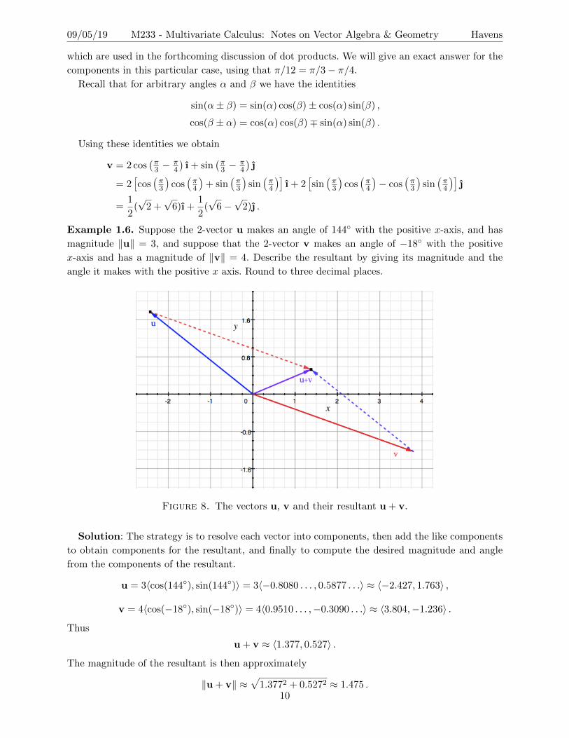
Example 1.6. Suppose the 2-vector u makes an angle of 144◦ with the positive x-axis, and has
magnitude ‖u‖ = 3, and suppose that the 2-vector v makes an angle of −18◦ with the positive
x-axis and has a magnitude of ‖v‖ = 4. Describe the resultant by giving its magnitude and the
angle it makes with the positive x axis. Round to three decimal places.
Figure 8. The vectors u, v and their resultant u + v.
Solution: The strategy is to resolve each vector into components, then add the like components
to obtain components for the resultant, and finally to compute the desired magnitude and angle
from the components of the resultant.
u = 3〈cos(144◦), sin(144◦)〉 = 3〈−0.8080 . . . , 0.5877 . . .〉 ≈ 〈−2.427, 1.763〉 ,
v = 4〈cos(−18◦), sin(−18◦)〉 = 4〈0.9510 . . . ,−0.3090 . . .〉 ≈ 〈3.804,−1.236〉 .
Thus
u + v ≈ 〈1.377, 0.527〉 .
The magnitude of the resultant is then approximately
‖u + v‖ ≈√
1.3772 + 0.5272 ≈ 1.475 .10
Page 13
09/05/19 M233 - Multivariate Calculus: Notes on Vector Algebra & Geometry Havens
Observe that the angle made with the positive x-axis can be computed using an arctangent of the
quotient of the component by the ı component:
θ ≈ arctan
Å0.527
1.377
ã≈ 20.951◦ .
In radians, the angle is approximately 0.366.
An intrepid student of geometry and trigonometry might recognize the angles and note that the
sines and cosines are exactly computable4. Such a student might give the following intimidating
but exact solution:
u =−3− 3
√5
4ı +
3»
10− 2√
5
4 , v =
»10− 2
√5 ı + (1−
√5) ,
u + v =1
4
Å−3− 3
√5 + 4
»10 + 2
√5
ãı +
Å1−√
5 +3
4
»10− 2
√5
ã
‖u + v‖ =
√25− 6
»10 + 2
√5 ,
θ = arctan
Ñ4− 4
√5 + 3
»10− 2
√5
−3− 3√
5 + 4»
10 + 2√
5
é.
This, together with the previous example, shows there is occasionally hope of obtaining exact
answers; be warned that one will generally not often encounter such special angles in the wild, nor
does one often need such exact answers in applications. Thus, for the question of resolving vectors
into components, and then recovering magnitudes and angles from a resultant, expect to obtain
only approximate answers, or complicated answers involving (possibly iterated) square roots.
§ 1.4. Problems
(1) If you are given three points, how many different ways can you complete them to a paral-
lelogram? If the three points have position vectors p, q and r, what are the vector formulae
for the possible position vectors of the final points of the parallelograms?
(2) Why are two linearly dependent vectors parallel?
(3) For each of the properties (3) - (8) of vectors listed in the proposition above, use pictures and
geometric reasoning to argue the truth of the properties without appealing to coordinate
algebra.
(4) Argue the absolute scalability property without using coordinates.
(5) Prove the absolute scalability property for vectors in V 3R using the coordinate formula for
magnitude.
(6) Prove the coordinate formula for the magnitude of a vector in V 3R using the pythagorean
theorem.
4One can compute the desired sines and cosines using double and half angle identities, from the knowledge that
cos 36◦ = (1 +√
5)/4, which happens to be half of the golden ratio and is also the apothem length of a regular
pentagon inscribed in the unit circle. To see the latter, cut the pentagon into ten triangles. See problems 14 and 15
below.
11
Page 14
09/05/19 M233 - Multivariate Calculus: Notes on Vector Algebra & Geometry Havens
(7) Prove the Pythagorean theorem. (Just kidding! But actually, if you can prove this visually,
that’s worth something...)
(8) For a fixed vector u in V 2R or V 3
R , what geometric object corresponds to the set of all vectors
parallel to u?
(9) For a fixed vector n ∈ V 3R , what is the geometric object corresponding to the set of all
vectors perpendicular to n?
(10) For a fixed pair of vectors u,v ∈ V 2R , what geometric object corresponds to the set of all
vectors x such that ‖x− u‖ = ‖x− v‖? What if we are in V 3R ?
(11) What geometric object corresponds to the set of all vectors of unit length in V 2R ? What
geometric object corresponds to the set of all vectors of unit length in V 3R ?
(12) For a vector u = u1ı + u2, give the coordinate form of the vector u′ = Rθu obtained by
rotating u counterclockwise by an angle θ.
(13) Use the previous exercise to describe equations relating the x, y coordinate system to an
x′, y′ coordinate system that is obtained by rotating the coordinate axes by an angle θ.
(14) For n = 3, 4, 5, and 6, give exact coordinates for position vectors for the vertices of a regular
n-gon (all sides equal length, all interior angles equal) inscribed in the unit circle, with one
vertex on the point (1, 0). Write down exact coordinates for displacement vectors giving the
sides of each n-gon, oriented so that walking along the sides of the n-gon, one circles the
origin counter-clockwise.
(15) For each n = 3, 4, 5, and 6 and regular n-gons as in the previous problem, what are the
sums of the displacement vectors giving the counter-clockwise oriented perimeter? What
are the perimeters? (You should give a positive scalar.) For each n-gon, what is the sum of
the position vectors of the vertices?
(16) Velocity is the derivative of position, and as position can be described as a vector quantity,
so too is velocity a vector quantity. If a particle is traveling around a unit circle at constant
unit speed, what, intuitively, should the velocity vector of the particle be at any given time?
(17) Acceleration is the derivative of velocity. For a particle traversing a circle as in the preceding
problem, what, intuitively, is the acceleration vector at any particular point in time?
(18) Suppose you are on a boat, traveling from a calm tributary into a river. The tributary meets
the river at a right angle, and you maintain a constant speed relative to the surface of the
water as you enter the main river. The river is flowing twice as fast as your speed relative to
its surface. You wish to travel to the point straight across from where you enter the river.
At what angle into the flow should you point your boat in order to get there? Why doesn’t
this depend on the width of the river?
12
Page 15
09/05/19 M233 - Multivariate Calculus: Notes on Vector Algebra & Geometry Havens
2. The Dot Product
We will define an operation which takes as input two vectors and outputs a scalar:
· : V nR × V n
R → R ,
a,b 7→ a · bIt is called the dot product or scalar product. The common approach to defining and studying
the dot product is to define it via a formula depending upon the coordinate representation in
rectangular coordinates. This has the advantage that it is immediately clear that the result is
defined in any finite number of dimensions. We will go a different route, studying first a geometric
problem that motivates the coordinate expression in 2 dimensions. We will then be able to argue
that the generalization of the coordinate expression continues to accomplish the geometric goal of
computing such a scalar product.
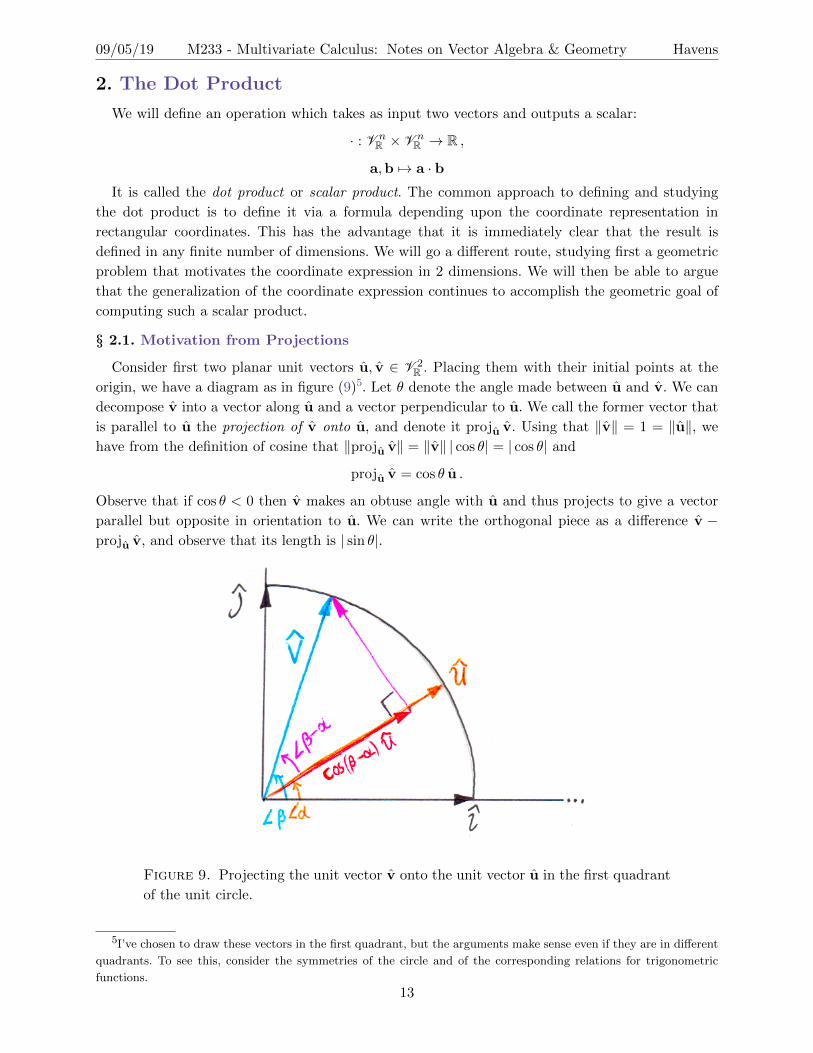
§ 2.1. Motivation from Projections
Consider first two planar unit vectors u, v ∈ V 2R . Placing them with their initial points at the
origin, we have a diagram as in figure (9)5. Let θ denote the angle made between u and v. We can
decompose v into a vector along u and a vector perpendicular to u. We call the former vector that
is parallel to u the projection of v onto u, and denote it proju v. Using that ‖v‖ = 1 = ‖u‖, we
have from the definition of cosine that ‖proju v‖ = ‖v‖ | cos θ| = | cos θ| and
proju v = cos θ u .
Observe that if cos θ < 0 then v makes an obtuse angle with u and thus projects to give a vector
parallel but opposite in orientation to u. We can write the orthogonal piece as a difference v −proju v, and observe that its length is | sin θ|.
Figure 9. Projecting the unit vector v onto the unit vector u in the first quadrant
of the unit circle.
5I’ve chosen to draw these vectors in the first quadrant, but the arguments make sense even if they are in different
quadrants. To see this, consider the symmetries of the circle and of the corresponding relations for trigonometric
functions.
13
Page 16
09/05/19 M233 - Multivariate Calculus: Notes on Vector Algebra & Geometry Havens
We can apply the above reasoning to obtain coordinate expressions for the unit vectors u and v
in terms of trigonometric functions. If α is the angle between u and ı and β is the angle between
v and ı then
u = cosα ı + sinα ,
v = cosβ ı + sinβ .
Writing u = u1ı + u2 and v = v1ı + v2, observe that
cos θ = cos(β − α) = cosα cosβ + sinα sinβ = u1v1 + u2v2 .
Thus, we can compute the cosine of the angle between two unit vectors from a simple expression
involving only the components.
Observe that if we scale v by a positive λ ∈ R to a non-unit vector v = λv = v′1ı + v′2 then the
projection proju v also scales, and the expression u1v′1 + u2v
′2 = λ(u1v1 + u2v2) instead computes
‖v‖ cos θ. If we scale u by a positive µ ∈ R to a non-unit vector u = µu = u′1ı + u′2, the projection
does not change length, but the formula for it is expressible as
‖v‖ cos(θ) u = ‖v‖ cos(θ)µ2u
µ2=
Ç‖u‖ ‖v‖ cos θ
‖u‖
åu
‖u‖.
The expression in the numerator of the coefficient on u = u/ ‖u‖ is what we will define to be the
dot product of u and v. Such a definition6 will still make sense in higher dimensions as two vectors
u,v ∈ V nR determine either a plane or a line, and one can measure the angle between them within
this smaller subspace, provided it is endowed with the same geometric notion of angle as the plane
R2.
Definition. Let u,v ∈ V nR be two vectors separated by an angle of θ ∈ [0, π]. Then the dot product
u · v is the scalar quantity
u · v = ‖u‖ ‖v‖ cos θ .
It follows that the cosine of the angle θ of separation between a pair of vectors u and v whose
dot product u · v is known is given by the expression
cos θ =u · v‖u‖ ‖v‖
.
However, to take advantage of this fact, we need another way to compute the dot product. We’ve
already seen that it can be done with coordinates when u and v are planar, and it is a simple leap
to generalize it.
6This is in some sense opposite to the usual approach, which is to define dot products algebraically, e.g. via
coordinates, and then show by the law of cosines that the dot product is proportional to the cosine of the angle
of separation via the product of magnitudes. One then defines angle in other contexts by first defining some inner
product (a product satisfying the algebraic properties of the dot product) and using it to define cosines and angles.
To arrest any concerns regarding the notion of angle, observe that since we are tacitly working in euclidean normed
topological vector spaces, we can define circles via the set of unit vectors in a 2-dimensional subspace, and we can
define the separation angle in radians between two vectors as the arc length of the smallest circular arc between the
corresponding unit vectors. Arc-length is of course computable provided we have a notion of integration, which we
always assume since this is a calculus course. We’ll describe arc-length computations in the next set of notes.
14
Page 17
09/05/19 M233 - Multivariate Calculus: Notes on Vector Algebra & Geometry Havens
§ 2.2. Coordinate Expressions
Our preceding discussion makes it clear that the dot product of u,v ∈ V 2R satisfies
u · v = u1v1 + u2v2 ,
where u1 = u · ı is the x component of u, u2 = u · is the y component of u, and similarly v1 = v · ı,v2 = v · . The nice result is that this generalizes easily:
Proposition. If u,v ∈ V 3R are given in coordinates as u = u1ı+u2+u3k and v = v1ı+v2+v3k,
then the coordinate expression for their dot products is
u · v = u1v1 + u2v2 + u3v3 .
More generally, if u = 〈u1, . . . un〉, v = 〈v1, . . . vn〉 are vectors in V nR , then the dot product is
computable as
u · v = u1v1 + . . .+ unvn =n∑i=1
uivi .
If you prefer, you may take the formula given in the preceding proposition as the definition, and
then prove that the geometric definition is equivalent. Armed with this definition, one can actually
compute projections and cosines of angles between vectors.
Recall, lines are said to be perpendicular or orthogonal to each other if they intersect and the
angle of separation between them at their point of intersection is a right angle. For vectors, if the
angle of separation is a right angle, the cosine vanishes, and so does the dot product. In fact, the
dot product is 0 if and only if either the vectors are perpendicular or at least one of the vectors is
the zero vector. We can define orthogonality for vectors then by the vanishing of the dot product.
The convention that 0 is orthogonal to all vectors allows us to succinctly say “two vectors have
vanishing dot product if and only if they are orthogonal”. When vectors u and v are perpendicular,
we sometimes write u ⊥ v.
On the other hand, vectors are said to be parallel if and only if one is a scalar multiple of the
other. In the parallel case, it is clear that the dot product is either the product of the two vectors’
magnitudes, if they have the same direction, or the negative of the product of their magnitudes, if
their directions are opposite. For parallel vectors u and v, we sometimes write u ‖ v.
Example 2.1. Show that the vectors u = ı − 8 + 10k and v = −2ı + + k are perpendicular.
Show that w = −4ı + 2− 2k is not parallel to v.
Solution: To show that u ⊥ v, we compute the dot product:
u · v = (ı− 8 + 10k) · (−2ı + + k) = (1)(−2) + (−8)(1) + (10)(1) = −2− 8 + 10 = 0 .
To show that v and w are not parallel, we can either check that one is not a multiple of the other,
or compute the angle between them from the dot product. For the first approach, one notes that if
they were parallel, there would be some λ ∈ R such that w = λv. Then
−4ı + 2− 2k = λ(−2ı + + k) = −2λı + λ + λk .
Then from the ı-components, we see that −4 = −2λ =⇒ λ = 2. for the component, this works,
but the k-component equation is −2 = λ. Since λ cannot be both 2 and −2, there can be no λ such
that w = λv.
Instead we can calculate the cosine of the angle of separation, which yields
cos θ =v ·w‖v‖ ‖w‖
=8 + 2− 2√
4 + 1 + 1√
16 + 4 + 4=
8
(√
6)(2√
6)=
2
3.
15
Page 18
09/05/19 M233 - Multivariate Calculus: Notes on Vector Algebra & Geometry Havens
If v ‖ w, then the cosine must be ±1, but instead we get 2/3, hence they are not parallel.
§ 2.3. Algebraic Properties
As with vector arithmetic, one can write down a litany of identities and properties satisfied by
the dot product. Arguing the truth of these identities from both the geometric and coordinate
definitions proves to be a most useful exercise. We list here the essential ones.
Proposition. Given vectors u,v,w in V nR and any scalar s ∈ R, the following properties hold:
(1) u · u = ‖u‖2 (norm compatibility)
(2) u · v = v · u (commutativity)
(3) (su) · v = s(u · v) = u · (su) (scalar/vector association)
(4) u · (v + w) = u · v + u ·w (distributivity)
(5) 0 · u = 0 (universal orthogonality of zero vector)
(6) |u · v| ≤ ‖u‖ ‖v‖ (Cauchy-Schwartz inequality)
Using the symmetry coming from (2), properties (3) and (4) can be combined into a single
identity as
u · (sv + w) = s(u · v) + u ·w .
Generally an operator L on vectors satisfying
L(u, sv + w) = s L(u,v) + L(u,w) , and
L(tu + v,w) = t L(u,w) + L(v,w)
is said to be bilinear. From the above properties it is clear that the dot product is a bilinear map
from pairs of real vectors to real scalars.
§ 2.4. Simple applications of the dot product
Returning to the subject of projections, and using that u · u = ‖u‖2, we can now state the
following general formula for projections:
Proposition. Given two vectors u,v ∈ V nR , the orthogonal projection of v onto u, also called the
component vector of v parallel to u is given by the formula
proju v =u · vu · u
u = (u · v)u = proju v ,
where u = u/√
u · u = u/ ‖u‖. The signed length of the projection, called the component of v in
the direction of u, is given by
compu v =u · v‖u‖
= u · v .
The component vector of v orthogonal to u is then given by v−proju v. That this is perpendicular
is easily verified with the dot product:
u · (v − proju v) = u · v − u · proju v
= u · v − u ·Å
u · vu · u
u
ã= u · v −
Åu · vu · u
ãu · u
= 0 .16
Page 19
09/05/19 M233 - Multivariate Calculus: Notes on Vector Algebra & Geometry Havens
Example 2.2. We will decompose the vector v = ı + 4 + 8k into components parallel and per-
pendicular to the vector u = 2ı − 4 + 4k. That is, we construct vectors v‖u and v⊥u such that
v⊥u · u = 0 and v‖u = proju(v). Following the preceding discussion, we thus compute
v‖u = proju(v) =
Åu · vu · u
ãu
=2− 16 + 32
4 + 16 + 16(2ı− 4 + 4k) =
18
36(2ı− 4 + 4k) = (ı− 2 + 2k)
v⊥u = v − proju(v) = ı + 4 + 8k− (ı− 2 + 2k)
= 6 + 6k .
Observe, we can easily check that v‖u · v⊥u = (ı− 2 + 2k) · (6 + 6k) = 0, and
v = ı + 4 + 8k = (ı− 2 + 2k)︸ ︷︷ ︸v‖u
+ (6ı + 6)︸ ︷︷ ︸v⊥u
.
Example 2.3. The projections of a vector u ∈ V 3R onto ı, and k respectively are just the
coordinate components:
u · ı = u1, u · = u2, u · k = u3 ,
u = u1ı + u2 + u3k = (u · ı)ı + (u · ) + (u · k)k = projı u + proj u + projk u .
Using the geometric interpretation of the dot product, we can compute the angles u makes with
each axis. Let α be the angle from the positive x axis to u, β the angle from the positive y axis to
u, and γ the angle from the positive z axis to u. These angles, called direction angles satisfy
cosα =u1
‖u‖cosβ =
u2
‖u‖cos γ =
u3
‖u‖.
Thus note that
u = ‖u‖Ä
cos(α) ı + cos(β) + cos(γ) kä.
In particular, any unit vector in R3 has components given by the three direction cosines!
We can use the dot product to find vectors perpendicular to a given vector u ∈ V 2R . If we write
u = 〈u1, u2〉, then we seek some vector v = 〈v1, v2〉 such that u · v = 0. Writing out the coordinate
expression for the product yields
u1v1 + u2v2 = 0 =⇒ u1v1 = −u2v2 .
Since we just want to find some vector perpendicular (after which we can scale to get others of
different lengths or in the opposite direction), we can make a choice: let’s set v1 = u2. We’ll see
that the result of our choice is we can find a vector v perpendicular to u with the same magnitude
as u. Indeed, our choice v1 = u2 then requires that v2 equal −u1 to satisfy the condition imposed
by the vanishing dot product. We can now easily check that v = 〈u2,−u1〉 is perpendicular to
u = 〈u1, u2〉, and the magnitudes are clearly the same since ‖v‖2 = v21 + v2
2 = u22 + (−u1)2 = ‖u‖2.
If you consider the slopes of the above vectors (the ratio of their y-components to their x-
components) then it should come as no surprise that v gives a vector perpendicular to u; the slope
of v is −u1u2
, which is the negative reciprocal of the slope u2u1
of u! Observe also that we could just
as well have taken −v to obtain another u-orthogonal vector of equal magnitude.17
Page 20
09/05/19 M233 - Multivariate Calculus: Notes on Vector Algebra & Geometry Havens
Example 2.4. The points P (−2, 3) and Q(4,−5) are opposite vertices of a square, meaning that
the line segment from P to Q is a diagonal of the square. Find the other two vertices of the square.
Solution:
Figure 10. The square with known vertices P and Q, and unknown vertices R and S.
Consider figure (10), which illustrates a square like the one described, where R and S are the
unknown vertices. Note that the two diagonals of the square have the same length and bisect
each other perpendicularly. By finding a vector perpendicular to the diagonalÐÐ⇀PQ, we get a vector
parallel toÐ⇀RS, which describes the displacement along the opposite diagonal. By finding position
vector m of the midpoint M between P and Q, and adding one halfÐ⇀RS, we can get the position
vector s for S, and similarly subtracting one halfÐ⇀RS from the midpoint position vector gives the
position vector r for R. Therefore we have
m = p +1
2
ÐÐ⇀PQ = p +
1
2(q− p) =
p + q
2
=1
2〈2,−2〉 = 〈1,−1〉 .
Note we computed the midpoint without writing downÐÐ⇀PQ, but we could just as well have computed
it using the first equality and the fact thatÐÐ⇀PQ = 〈6,−8〉, giving the equivalent computation
m = 〈−2, 3〉+1
2〈6,−8〉 = 〈−2, 3〉+ 〈3,−4〉 = 〈1,−1〉 .
Now, from the discussion preceding this example, we know thatÐ⇀RS = 〈8, 6〉 ,
and so
s = m +1
2
Ð⇀RS = 〈1,−1〉+ 〈4, 3〉 = 〈5, 2〉 , and
r = m− 1
2
Ð⇀RS = 〈1,−1〉 − 〈4, 3〉 = 〈−3,−4〉 .
Thus the other vertices of the square are S(5, 2) and R(−3,−4).
Projections and dot products are commonly applied in physics problems such as using Newton’s
laws to calculate forces in static and dynamic problems. By a velocity vector, we shall mean a
vector describing the motion of an object giving the direction of its movement at that instant, with
magnitude equal to the speed of the object. Velocity is the derivative of the position vector. The18
Page 21
09/05/19 M233 - Multivariate Calculus: Notes on Vector Algebra & Geometry Havens
derivative of velocity is acceleration, and describes both changes in direction and changes in speed.
Newton’s second law of motion states that force is proportional to acceleration via mass: if F is
a force vector applied to an object of mass m, and the object accelerates due to this force with
acceleration vector a7, then
F = ma .
This assumes no other forces are acting on the object; in nature we do not encounter such circum-
stances. The correct way to understand this is as follows. Since force is a vector, we can really view
F as representing the vector sum of all forces acting on the object within a particular inertial frame
of reference8. By this we mean there is a coordinate system within which we measure the forces
acting on objects, and if they sum to 0 in this coordinate system, there is no net acceleration of
the objects to which the forces were applied. Some authors clarify this by writing Newton’s second
law as
ΣF = ma ,
where the Σ reminds us that we are examining the net force, which is a sum of various forces acting
on the object. The acceleration vector a is taken to mean the acceleration relative to the inertial
coordinate system.
In the simplest applications, one considers the case where an object is at rest or undergoing
linear motion at a constant speed within an inertial frame of reference, and thus the acceleration is
0, and the forces must balance out in all directions. This is called a static system.9 We’ll consider
an example of a simple static system that demonstrates the use of projections.
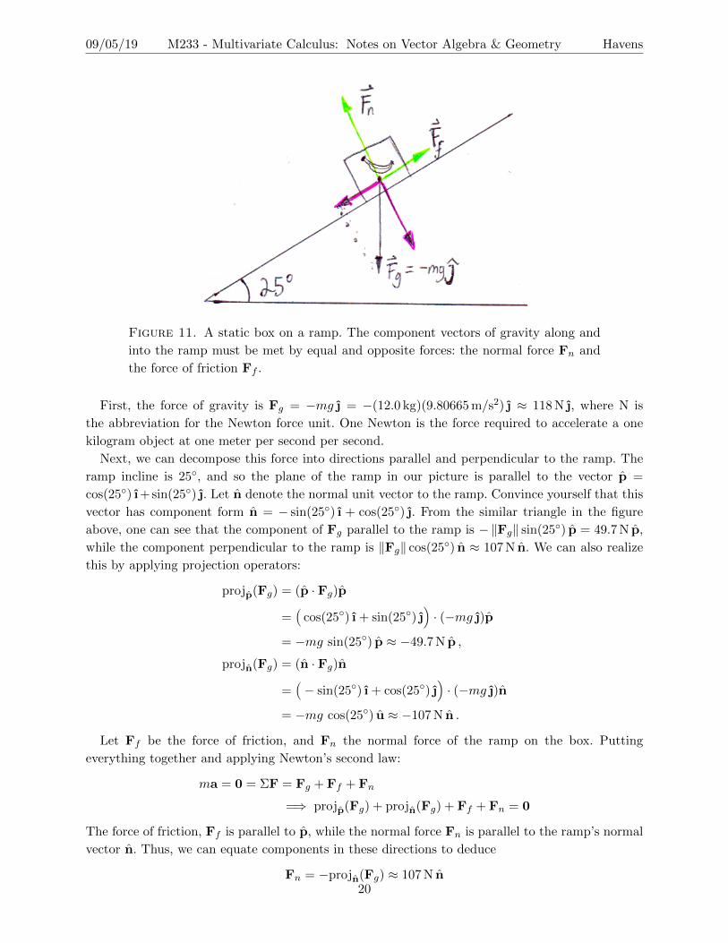
Example 2.5. A box is sitting on a ramp, and does not slide down the ramp. The ramp is inclined
at 25.0◦ relative to the horizontal. If the box has a mass of 12.0 kilograms, what is the acting force
of friction keeping the box from sliding? Assume that gravity exerts a force equal to the mass of
the box times g = 9.80665m/s2 in a direction perpendicular to the horizontal.
Solution: The first step is to understand what forces act on the box, and in what directions.
There is the downward force exerted by gravity, there is the normal force exerted by the ramp
perpendicular to the incline, and there is a force of friction parallel to the plane of incline. The
normal force must exist else the box would accelerate into the ramp, while the force of friction
is what prevents the box from sliding along the ramp. To understand these, we decompose the
gravitational force into components parallel and perpendicular to the ramp, and apply Newton’s
second law to the sum of forces, with a net acceleration of 0. A visual aid helps keep track of this
information, as in figure 11 below.
7Recall, acceleration is the derivative of velocity, which is the derivative of position. Thus, for a particle with
position r(t) at time t, the acceleration is a(t) = dvdt
= d2rdt2
. Here, the position r(t), the velocity v(t) = drdt
, and the
acceleration a(t) are each vector valued functions. The next set of notes concerns vector valued functions and their
derivatives, and explores velocity and acceleration in greater depth.8The name inertial reference frame is itself a reference to Newton’s first law of motion: the law of inertia. The
modern statement is that an object with no net force acting upon it will experience no net acceleration in such a
reference frame. The term inertia describes the tendency to resist change (in this case, in velocity): as it is often
quoted “an object at rest will remain at rest until an outside force acts upon it, and an object in motion will stay in
motion until an outside force acts upon it.”9Though the word “static” conjures an image of motionlessness, our definition permits an object moving at constant
velocity. Why then call it “static”? Well, if the object has velocity v, we can choose a new inertial reference system
that moves along with the object at constant velocity v relative to the old reference frame. Then in this frame of
reference, the object is motionless, i.e., static!
19
Page 22
09/05/19 M233 - Multivariate Calculus: Notes on Vector Algebra & Geometry Havens
Figure 11. A static box on a ramp. The component vectors of gravity along and
into the ramp must be met by equal and opposite forces: the normal force Fn and
the force of friction Ff .
First, the force of gravity is Fg = −mg = −(12.0 kg)(9.80665 m/s2) ≈ 118 N , where N is
the abbreviation for the Newton force unit. One Newton is the force required to accelerate a one
kilogram object at one meter per second per second.
Next, we can decompose this force into directions parallel and perpendicular to the ramp. The
ramp incline is 25◦, and so the plane of the ramp in our picture is parallel to the vector p =
cos(25◦) ı+sin(25◦) . Let n denote the normal unit vector to the ramp. Convince yourself that this
vector has component form n = − sin(25◦) ı + cos(25◦) . From the similar triangle in the figure
above, one can see that the component of Fg parallel to the ramp is −‖Fg‖ sin(25◦) p = 49.7 N p,
while the component perpendicular to the ramp is ‖Fg‖ cos(25◦) n ≈ 107 N n. We can also realize
this by applying projection operators:
projp(Fg) = (p · Fg)p
=Ä
cos(25◦) ı + sin(25◦) )· (−mg )p
= −mg sin(25◦) p ≈ −49.7 N p ,
projn(Fg) = (n · Fg)n
=Ä− sin(25◦) ı + cos(25◦)
)· (−mg )n
= −mg cos(25◦) u ≈ −107 N n .
Let Ff be the force of friction, and Fn the normal force of the ramp on the box. Putting
everything together and applying Newton’s second law:
ma = 0 = ΣF = Fg + Ff + Fn
=⇒ projp(Fg) + projn(Fg) + Ff + Fn = 0
The force of friction, Ff is parallel to p, while the normal force Fn is parallel to the ramp’s normal
vector n. Thus, we can equate components in these directions to deduce
Fn = −projn(Fg) ≈ 107 N n20
Page 23
09/05/19 M233 - Multivariate Calculus: Notes on Vector Algebra & Geometry Havens
Ff = −projp(Fg) ≈ 49.7 N p .
In particular, the effective force of friction on the box is about 49.7 Newtons upward along the
ramp.
Another physics context in which the dot product plays an important role is work. Work is
commonly described as force times displacement, but when this definition is given, it is tacit that
both force and displacement are vectors, and somehow the work you measure is how much force
works to produce how much linear displacement10. In particular, if you apply lots of force and
the object moves at an angle to the direction in which you applied the force, the work will only
account for the component of effective force, which is parallel to the object’s motion. Thus, a
careful definition of work inn the setting of constant applied force is as the dot product of force and
displacement, which equals the real product of the effective force in the direction of the displacement
it causes. So, if you apply a force F to an object, displacing it by a vector s, then the work is the
scalar
W = F · s .If the force varies across the displacement, then one needs to account for the change of the
force along the object’s trajectory, and so naturally some calculus becomes necessary. In partic-
ular, one must consider force fields along curved trajectories, and integrate to find net work. The
corresponding mathematical objects needed are “vector-valued functions” r : R → R3 to describe
the trajectory11, and “vector fields” F : V 3R → R3 to describe the force at different points of space.
Then one defines work via a gadget called a line integral. This idea is explored in the final unit of
this course (see the later notes on line integrals).
Example 2.6. A force of 100 Newtons is applied to a box on a floor. The force is applied at
an angle, so that a component of the force is upwards, with F making an angle of 32◦ with the
horizontal. Find the work done on the box if it is dragged 6.5 meters, in Joules (1 Joule is the work
to move an object 1 meter with an effective applied force of 1 Newton, i.e. 1 J = 1 N × 1 m.)
Solution: Applying the geometric interpretation of the dot product to compute work from its
definition:
W = F · s = ‖F‖ ‖s‖ cos 32◦ = (100 N)(6.5 m)(0.848 . . .) ≈ 550 N m = 550 J .
Equivalently, by computing the projection of F onto s and then multiplying by ‖s‖, we work directly
with the effective force coming from the component parallel to the displacement, and recover the
same calculation.
§ 2.5. Problems
(1) (Do this whole problem only if you want lots of practice computing)
Compute all possible dot products involving the vectors a = 〈1, 1, 1〉, b = 〈−2, 3,−3〉,c = 〈−1, 4, 7〉, u = 〈1/2,−1/3, 1/6〉, v = 〈0, 9, 9〉, and w = 〈−7, 6, 0〉, and compute all
possible projections and the complimentary orthogonal component vectors.
11Here, we can identify R3 with V 3R by considering each point along the trajectory as being determined by a
position vector; in practice we describe such functions parametrically as a triple or real valued functions r(t) =
x(t) ı + y(t) + z(t) k.
21
Page 24
09/05/19 M233 - Multivariate Calculus: Notes on Vector Algebra & Geometry Havens
(2) Give a concrete example showing that the dot product does not have the cancellation
property, i.e. show that u ·v = u ·w does not imply that v = w. For a fixed pair u,v ∈ V 3R ,
describe geometrically the set of all vectors w ∈ V 3R such that u ·w = u · v.
(3) For real numbers, it is well known that multiplication satisfies an associative property:
a(bc) = abc = a(bc) for any a, b, c ∈ R. Why is there no associative property of the dot
product? What’s wrong with writing a · (b · c) = a · b · c = (a · b) · c?
(4) By a diagonal of a cube, we mean the line segment from one vertex of a cube to the farthest
vertex across the cube. By a diagonal of a cube’s face, we mean the diagonal of the square
face from one vertex to the opposite vertex of that face.
(a) Find the lengths of the diagonals of a cube and diagonals of faces in terms of the side
length of a cube.
(b) Find the angles between a diagonal of a cube and an adjacent edge of the cube.
(c) Each diagonal of the cube is adjacent to how many face diagonals? Find the angle
between a diagonal of a cube and an adjacent face diagonal.
(5) For u = u1ı + u2 and v = v1ı + v2, write the magnitude of the resultant u + v in terms
of the components of u and v, and then give formulae for the angles made between the
resultant and each of ı, , u and v.
(6) A 10.5 kilogram box is sliding down a ramp, which is inclined at 28.2◦ relative to the
horizontal. Suppose the force of friction of the ramp on the sliding box has magnitude
proportional to the normal force exerted by the ramp on the box, with constant of pro-
portionality µ = 0.155 (such a µ is called the coefficient of friction). Assuming, as in the
example above, that gravity exerts a downward force equal to the mass of the box times
g = 9.80665m/s2, find the acceleration of the box along the ramp. Your answer should be
rounded so as to contain 3 significant figures. You may of course neglect things like air
resistance that would complicate the assumption of constant acceleration.
(7) A 5.25 kilogram sculpture is suspended from a gallery ceiling by three wires which meet at
a single hook on the sculpture. If the origin is placed at the hook, then one wire is parallel
to 1.0ı + 1.6 + 1.0k, one wire is parallel to 2.0ı− 3.0 + 2.0k and the last wire is parallel to
−3.0ı + 0.25 + 3.0k. If the sculpture hangs 1.57 meters below the ceiling of the gallery, find
the lengths of each of the wires. Assuming the sculpture is non-kinetic, find the tension in
each wire.
(8) Three exuberant dogs are recreationally pulling a sled around in a snow-covered field, but
they are not quite coordinated. They exert forces along 3 different directions, but manage
to pull the sled in a straight line briefly before it begins to veer about wildly. Suppose that
during the linear motion, one dog exerts a constant force of 165 Newtons of force in the
direction of the vector −1.00ı+1.80+0.60k, one dog exerts a constant force of 184 Newtons
parallel to the vector 2.00ı + 2.20 + 0.50k, and the final dog exerts a constant force of 240
Newtons along the vector 2.40ı + 0.70k.
(a) Assuming the sled does not lift off of the snow, and the only forces acting upon it are
those due to the dogs, gravity and friction, determine a unit vector in the direction of
the sled’s displacement.22
Page 25
09/05/19 M233 - Multivariate Calculus: Notes on Vector Algebra & Geometry Havens
(b) Compute the work each dog does if the sled is displaced 8.00 meters along the direction
described in part (a).
(c) Compute the total work done by the dogs on the sled.
(d) (Challenge) If the sled is packed to weigh 65.0 kilograms, the coefficient of friction
between the sled blades and the snow is µ = 0.007, and the dogs accelerate so that
the forces described above are the tensions maintained in the ropes during the linear
motion of the sled, determine the equations of the sled’s motion for the straight line
displacement. How many seconds does it take to complete the 8.00 meter run? You
may assume g = 9.80665m/s2, and use 3 significant figures for your final answer.
(9) Let a, b, c ∈ R+ be positive real numbers giving the lengths of the sides of a triangle. Suppose
the sides of length a and b are separated by an interior angle of θ. Then the Law of cosines
states that
c2 = a2 + b2 − 2ab cos θ .
Prove the Law of cosines using vector algebra. (Hint: describe the sides using vectors, and
compute the square of c geometrically by a dot product.)
(10) Prove that, for any u,v ∈ V nR ,
2 ‖u‖2 + 2 ‖v‖2 = ‖u + v‖2 + ‖u− v‖2 , and
u · v =1
4
(‖u + v‖2 − ‖u− v‖2
)(11) Consider linearly independent vectors u,v ∈ V 2
R , and let P be the parallelogram whose
sides they span. Under what conditions are the diagonals of P orthogonal?
(12) Demonstrate via vector algebra that the diagonals of a parallelogram always bisect each
other.
(13) For a line through the origin in the direction of u ∈ V 2R , use the projection operator to give
an expression for the reflection of a vector x through the line.
(14) Prove the Cauchy-Schwartz inequality for the dot product (property (6) in the proposition
above).
(15) Describe a procedure, using the dot product, to generate from a list of vectors v1, . . .vn ∈V nR , a new list u1, . . . , un ∈ V n
R such that
‖ui‖ = 1 , i = 1, . . . n ,
ui · uj = 0 if i 6= j .
Such a set is called an orthonormal basis. The vectors ı, , and k form an orthonormal basis
of V 3R .
(16) Use the procedure of the preceding problem to generate an orthonormal basis from the
vectors 〈4,−4, 7〉, 〈1, 1, 1〉, and 〈−3, 4,−5〉.
23
Page 26
09/05/19 M233 - Multivariate Calculus: Notes on Vector Algebra & Geometry Havens
(17) Using the algebraic properties of the dot product and the geometric definition, prove the
coordinate expression
u · v = u1v1 + u2v2 + u3v3
Generalize your proof to the expression
u · v = u1v1 + . . .+ unvn =n∑i=1
uivi
by using an orthonormal basis e1, . . . , en for V nR .
24
Page 27
09/05/19 M233 - Multivariate Calculus: Notes on Vector Algebra & Geometry Havens
3. Cross Product
While we have one notion of “product” for vectors, it doesn’t really meet the criteria that
the average mathematician would ideally desire in a product operation. Namely, the dot product
is a map from a pair of vectors to a scalar. But one might wonder if there is a map with useful
properties taking a pair of vectors to a vector in the same vector space. By a stroke of mathematical
fortune, in three dimensions such a product exists and its properties make it useful in the study of
lines, planes, areas, volumes, rotational mechanics, and spatial rotations. Its origins, like the ı, , k
notation for coordinate vectors, harken back to an historical attempt by William Rowan Hamilton
to generalize the success of complex number arithmetic in describing planar geometry to a spatial
analog via hypercomplex numbers. This is discussed in further depth in a later (optional) section
on quaternions. Fortunately, now we can approach a definition of the product in various modern
ways, all grounded in perspectives that will find use.
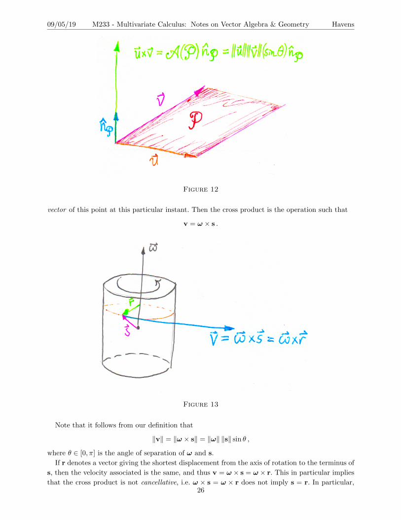
§ 3.1. Geometric Definition
We will rely on geometry to give a definition which is a priori not particularly helpful in com-
putations, but which will nonetheless give us a map
× : V 3R × V 3
R → V 3R .
Given a pair of nonzero vectors u,v ∈ V 3R , then either they span a plane, or they are parallel (and
thus, span only a line). In the event that they span only a line or at least one vector is the zero
vector, we will define their product to return the zero vector. On the other hand, if they span a
plane, we will determine a vector perpendicular to that plane whose direction will depend on the
right hand rule, and whose magnitude encodes geometric information about u and v. In particular,
for u and v not parallel, let P be the parallelogram spanned by them (so if u and v are placed
emanating from the origin, P has vertices with position vectors 0, u, v and u + v). The right
hand rule furnishes a unique unit vector nP normal to this parallelogram (and so, to both u and
v) such that (u,v, nP) is a right-handed triple (if we insisted on having a left-handed triple, we’d
get −nP). Note that we could get an expression in coordinates for nP by writing down coordinate
equations from the condition nP · u = 0 = nP · v, solving up to a constant, then choosing the
constant to ensure that the normal vector had unit length and that we had a right-handed triple.
Now, let A(P) be the area of the parallelogram. You should convince yourself (draw a picture!)
that this area is equal to ‖u‖ ‖v‖ sin θ where θ ∈ (0, π) is the angle of separation of u and v.
Definition. For u,v ∈ V 3R , the cross product is the vector defined by the following conditions:
(1) u× v = 0 whenever u and v are parallel.
(2) For u and v linearly independent, with P, nP , A(P), and θ as above,
u× v := A(P)nP = ‖u‖ ‖v‖ sin(θ) nP .
§ 3.2. Physical Definition
This definition is adapted from Bressoud’s Second Year Calculus. We consider a rigid object,
with center of mass at the origin, rotating around an axis. Let ω denote an angular velocity vector,
defined as follows: ω points along the axis of rotation from the center of mass such that, looking
back at the center of mass from the tip of ω, one sees the rotation as counter-clockwise, and ‖ω‖is the angular speed of rotation, measured in radians per second. Fix a moment in time. Now, let s
be a position vector locating a point of the object at this moment, and let v be the linear velocity25
Page 28
09/05/19 M233 - Multivariate Calculus: Notes on Vector Algebra & Geometry Havens
Figure 12
vector of this point at this particular instant. Then the cross product is the operation such that
v = ω × s .
Figure 13
Note that it follows from our definition that
‖v‖ = ‖ω × s‖ = ‖ω‖ ‖s‖ sin θ ,
where θ ∈ [0, π] is the angle of separation of ω and s.
If r denotes a vector giving the shortest displacement from the axis of rotation to the terminus of
s, then the velocity associated is the same, and thus v = ω × s = ω × r. This in particular implies
that the cross product is not cancellative, i.e. ω × s = ω × r does not imply s = r. In particular,26
Page 29
09/05/19 M233 - Multivariate Calculus: Notes on Vector Algebra & Geometry Havens
despite having a vector valued product operation for three dimensional vectors, there is no way to
define division for this product.12
In physics, the cross product appears frequently when dealing with rotational phenomena. An
elementary example is the definition of torque. Given a lever arm let ` be a vector from the fulcrum
to the end, and consider a force F applied to the lever arm at the terminal point of `. Then torque
is the vector quantity
τ := `× F .
§ 3.3. Algebraic and Geometric properties
A real test of geometric fluency with 3-dimensional vectors is to try and use the above two
definitions of the cross product to obtain a list of algebraic properties analogous to those of the dot
product. There will however be some important differences. The cross product is anti-commutative
and non-associative. It does however satisfy bilinearity properties like those of the dot product.
The proposition below lists the most important algebraic properties of the cross product. See if you
can rediscover or prove them by appealing to geometric and physical reasoning.
Proposition. Given vectors u,v,w in V 3R and any scalar s ∈ R, the following properties hold:
(1) u× v = −(v × u) (anti-commutativity)
(2) (su)× v = s(u× v) = u× (su) (scalar/vector association)
(3) u× (v + w) = u× v + u×w (left distributivity)
(4) (u + v)×w = u×w + v ×w (right distributivity)
(5) u× u = 0 (vanishing on co-linear pairs)
(6) 0× u = 0 (universal co-linearity of zero vector)
(7) u× (v ×w) + v × (w × u) + w × (u× v) = 0 (Jacobi identity)
The anti-commutative property is sometimes called skew-symmetry. The cross product deter-
mines a skew-symmetric bilinear map from pairs of 3-dimensional real vectors to 3-dimensional real
vectors. One might wonder if there are skew-symmetric bilinear products of vectors in V nR taking
values in V nR , for n other than 3. The initially startling answer is that these products are rare,
occurring only in dimensions n = 3 and n = 7 (there’s of course the usual product of 1-dimensional
real vectors, i.e. the usual product on real numbers, but that operation is commutative.)
§ 3.4. Deriving Coordinate Expressions
Given the properties of the cross product listed in the preceding proposition, we can apply our
definitions to obtain a computational rule for calculating the cross product in coordinates.
First, we consider the cross products of the coordinate basis vectors ı, and k. Note that their
are 9 possible ways to form cross products from these. Property (5) implies that 3 of these, namely
i× i, j× j, k× k, are all equal to 0. The remaining 6 products form three pairs, related according
to property 1, by reversal. For example, since ı and span a unit square with k the right-handed
unit normal to this square, we have from the geometric definition that
ı× = k = −× ı .
12The question of which vector spaces over R admit the structure of a real normed division algebra is closely
connected to the existence of cross products. The only vector spaces admitting such structures occur in dimensions
1, 2, 4, and 8, corresponding to the real numbers, complex numbers, quaternions, and octonions respectively. Cross
products, which fit into the scheme discussed below of skew symmetric bilinear products taking values orthogonal to
their arguments, are produced in dimensions 3 and 7 as a by-product of the normed division algebra structures in
dimensions 4 and 8.
27
Page 30
09/05/19 M233 - Multivariate Calculus: Notes on Vector Algebra & Geometry Havens
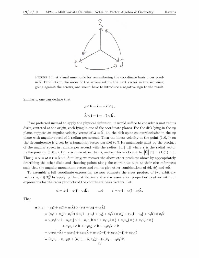
Figure 14. A visual mnemonic for remembering the coordinate basis cross prod-
ucts. Products in the order of the arrows return the next vector in the sequence;
going against the arrows, one would have to introduce a negative sign to the result.
Similarly, one can deduce that
× k = ı = −k× ,
k× ı = = −ı× k .
If we preferred instead to apply the physical definition, it would suffice to consider 3 unit radius
disks, centered at the origin, each lying in one of the coordinate planes. For the disk lying in the xy
plane, suppose an angular velocity vector of ω = k, i.e. the disk spins counterclockwise in the xy
plane with angular speed of 1 radian per second. Then the linear velocity at the point (1, 0, 0) on
the circumference is given by a tangential vector parallel to . Its magnitude must be the product
of the angular speed in radians per second with the radius, ‖ω‖ ‖r‖ where r is the radial vector
to the position (1, 0, 0). But r is none other than ı, and so this works out to∥∥∥k∥∥∥ ‖ı‖ = (1)(1) = 1.
Thus = v = ω× r = k× ı. Similarly, we recover the above other products above by appropriately
describing the other disks and choosing points along the coordinate axes at their circumferences
such that the angular momentum vector and radius give other combinations of ±ı, ± and ±k.
To assemble a full coordinate expression, we now compute the cross product of two arbitrary
vectors u,v ∈ V 3R by applying the distributive and scalar association properties together with our
expressions for the cross products of the coordinate basis vectors. Let
u = u1ı + u2 + u3k , and v = v1ı + v2 + v3k .
Then
u× v = (u1ı + u2 + u3k)× (v1ı + v2 + v3k)
= (u1ı + u2 + u3k)× v1ı + (u1ı + u2 + u3k)× v2 + (u1ı + u2 + u3k)× v3k
= u1v1i× i + u2v1j× i + u3v1k× i + u1v2i× j + u2v2j× j + u3v2k× j
+ u1v3i× k + u2v3j× k + u3v3k× k
= u2v1(−k) + u3v1 + u1v2k + u3v2(−ı) + u1v3(−) + u2v3ı
= (u2v3 − u3v2)ı + (u3v1 − u1v3) + (u1v2 − u2v1)k .28
Page 31
09/05/19 M233 - Multivariate Calculus: Notes on Vector Algebra & Geometry Havens
§ 3.5. Determinants and Areas
A popular mnemonic for the cross product’s component formula can be given in terms of an
object from linear algebra called a determinant. Determinants are defined for square matrices, which
may be thought of as collections of vectors. Determinants characterize the linear independence of
collections of vectors, and give a way to compute volumes of objects determined by collections of
vectors. The 2-dimensional case of the determinant characterizes when two vectors are not parallel,
and gives us a formula for the area of a parallelogram in terms of the vectors spanning its sides. It
shows up in explicit solutions for the intersection of two lines, and it turns out the coefficients in
our cross product formula are all determinants of certain 2× 2 matrices.
To see where determinants come from, you could try solving the system of equationsax+ by = e
cx+ dy = f.
After a little algebra, you should find that
x =de− bfad− bc
, y =af − cead− bc
,
provided the fractions given are defined. In particular, the quantity ad − bc cannot be zero if you
wish to have a unique solution corresponding to a point of intersection. We say that ad− bc is the
determinant associated to this linear system of equations. Traditionally, determinants are defined
for square matrices, so we shall look briefly at those in the simplest cases of 2×2 and 3×3 matrices.
One often rewrites such a linear system with a matrix-vector product, as follows:ña b
c d
ô ñx
y
ô=
ñe
f
ô,
where the square matrix acts on the vector 〈x, y〉 (written above in column notation) by the formulaña b
c d
ô ñx
y
ô=
ñax+ by
cx+ dy
ô.
Note that each entry of the resulting vector is the dot product of a row vector with the column
vector that the matrix is acting on. By equating this with the constant vector 〈e, f〉, and thus
separately equating their components, we recover the linear system of equations above.
We will define the determinant of the matrixña b
c d
ôto be ad− bc. One often writes ∣∣∣∣∣ a b
c d
∣∣∣∣∣ = ad− bc .
This definition is more than merely a convenient shorthand. One sees from the above algebra that
a linear system associated to this matrix possesses a unique solution if and only if the determinant
is nonzero. The determinant is nonzero if and only if the vectors 〈a, b〉 and 〈c, d〉 are linearly
independent. (for two vectors this means not parallel). Why might this number ad − bc capture
that fact?
It turns out, ad − bc is the signed area of the parallelogram with one vertex the origin and
sides given by the vectors 〈a, b〉 and 〈c, d〉. One can prove this using a little bit of trigonometry
(try writing the vectors in polar coordinates, compute the determinant, then try to relate it via a29
Page 32
09/05/19 M233 - Multivariate Calculus: Notes on Vector Algebra & Geometry Havens
trigonometric identity to the formula for parallelogram area.) Of course, if the vectors are parallel,
they do not determine a true parallelogram, and one can think of the ‘area enclosed” as 0.
It should then be unsurprising that determinants show up in our coordinate expression for the
cross product, since we defined it so that its length was the area of a parallelogram! The popular
mnemonic involves 3×3 determinants, though. Thankfully, a 3×3 determinant is built as a weighted
sum of three 2× 2 determinants.
Define a 3× 3 determinant to be∣∣∣∣∣∣∣a1 a2 a3
b1 b2 b3c1 c2 c3
∣∣∣∣∣∣∣ = a1
∣∣∣∣∣ b2 b3c2 c3
∣∣∣∣∣− a2
∣∣∣∣∣ b1 b3c1 c3
∣∣∣∣∣+ a3
∣∣∣∣∣ b1 b2c1 c2
∣∣∣∣∣= a1b2c3 − a1b3c2 − a2b1c3 + a2b3c1 + a3b1c2 − a3b2c1 .
By an abuse of notation, we place along the first row ı, , and k instead of a1, a2 and a3, and
along the second and third rows we place the components of the vectors we wish to cross, with the
first vector of the product having its entries in the second row, and the last vector having its entries
in the final row. This gives us
u× v =
∣∣∣∣∣∣∣ı k
u1 u2 u3
v1 v2 v3
∣∣∣∣∣∣∣ =
∣∣∣∣∣ u2 u3
v2 v3
∣∣∣∣∣ ı−∣∣∣∣∣ u1 u3
v1 v3
∣∣∣∣∣ +
∣∣∣∣∣ u1 u2
v1 v2
∣∣∣∣∣ k= (u2v3 − u3v2)ı + (u3v1 − u1v3) + (u1v2 − u2v1)k .
We’ll shortly connect this mnemonic with the volume interpretation of determinants, but for
the moment, we present an example involving the geometric interpretation of the cross product in
terms of area.
Example 3.1. Find the area of the triangle with vertices P (−1,−2,−3),Q(1,−1,−3) andR(1, 2, 0).
Solution: The triangle’s sides are spanned by displacement vectorsÐÐ⇀PQ = q− p = 〈2, 1, 0〉 and
ÐÐ⇀PR = r− p = 〈2, 4, 3〉. The area of the triangle is half of the area of the parallelogram spanned by
these vectors. Thus, we compute ‖ÐÐ⇀PQ×
ÐÐ⇀PR‖/2:∣∣∣∣∣∣∣
ı k
2 1 0
2 4 3
∣∣∣∣∣∣∣ = 3ı− 6 + 6k .
1
2‖ÐÐ⇀PQ×
ÐÐ⇀PR‖ =
1
2
√9 + 36 + 36 =
9
2.
Thus the area of the triangle is 9/2.
§ 3.6. Triple Products
Consider a triple of linearly independent vectors a,b, c ∈ V 3R , placed with tails at the origin of
R3. Each pair taken from this triple spans a parallelogram with one vertex at 0, and viewed as
position vectors, a, b, c, and 0 together with the sums a + b, b + c, c + a, and a + b + c, form the
vertices of a solid called a parallelepiped. The points on the interior of the parallelepiped form the
set W = {t1a + t2b + t3c | 0 ≤ ti ≤ 1, i = 1, 2, 3}. We wish to give an expression for the volume of
the parallelepiped.
Reasoning geometrically, this volume should equal the area of any one of the parallelogram faces
times an altitude perpendicular to that face, i.e. a line segment starting with the chosen face and30
Page 33
09/05/19 M233 - Multivariate Calculus: Notes on Vector Algebra & Geometry Havens
Figure 15. A view of a parallelepiped in R3.
ending in the opposite face, meeting each orthogonally. We can use a cross product of two of our
vectors to compute the area of one of the faces, and a little geometric reasoning allows us to see
that scaling the cross product by the length of the remaining vector times the cosine of the angle of
separation between the cross product and this remaining vector gives us, up to a sign, an expression
equal to the product of the area of a face with the length of an altitude. Thus, the volume of the
parallelepiped is given by the absolute value of a scalar triple product
V = |(a× b) · c| .
If the triple is right handed, the scalar triple product is positive, and gives the volume straight
away. Convince yourself of the following:
Proposition. For a given triple of vectors a,b, c ∈ V 3R , the possible rearrangements of scalar triple
products yield only two values, one of which is the volume of the associated parallelepiped, and the
other the negative of this volume. The positive arrangements for a right-handed triple (a,b, c) are
(a× b) · c , (c× a) · b , (b× c) · a .
The negative arrangements are
(a× c) · b , (b× a) · c , (c× b) · a .
Let’s examine the triple product with our coordinate expressions for the dot and cross products.
Consider, e.g. a · (b×c) with a = a1ı +a2 +a3k, b = b1ı + b2 + b3k, and c = c1ı + c2 + c3k. Then
a · (b× c) =Äa1ı + a2 + a3k
ä·((b2c3 − b3c2)ı− (b1c3 − b3c1) + (b1c2 − b2c1)k
)= a1(b2c3 − b3c2)− a2(b1c3 − b3c1) + a3(b1c2 − b2c1)
= a1
∣∣∣∣∣ b2 b3c2 c3
∣∣∣∣∣− a2
∣∣∣∣∣ b1 b3c1 c3
∣∣∣∣∣+ a3
∣∣∣∣∣ b1 b2c1 c2
∣∣∣∣∣=
∣∣∣∣∣∣∣a1 a2 a3
b1 b2 b3c1 c2 c3
∣∣∣∣∣∣∣ .This demonstrates that 3× 3 determinants compute volumes, up to sign!
31
Page 34
09/05/19 M233 - Multivariate Calculus: Notes on Vector Algebra & Geometry Havens
Example 3.2. Find the volume of the parallelepiped with edges spanned by the vectors 〈−2, 1, 2〉,〈2, 1,−2〉 and 〈−1, 2,−1〉.
Solution: we compute the determinant∣∣∣∣∣∣∣−2 1 2
2 1 −2
−1 2 −1
∣∣∣∣∣∣∣ = 2 + 2 + 8− (−2)− (8)− (−2) = 8 .
Here, the 3× 3 determinant was calculated using the formula∣∣∣∣∣∣∣a1 a2 a3
b1 b2 b3c1 c2 c3
∣∣∣∣∣∣∣ = a1b2c3 + a2b3c1 + a3b1c2 − c1b2a3 − a2b3c1 − c3b1a2 .
Figure 16. The volume of this parallelepiped is 8.
There is another type of triple product to consider, the vector triple product. For example, one
might consider products of the form
a× (b× c) , and (a× b)× c .
These are not in general equal.
Proposition. For a,b, c ∈ V 3R , the vector triple product satisfies
a× (b× c) = (a · c)b− (a · b)c .
This is sometimes written as a × (b × c) = b(a · c) − c(a · b), leading to the mnemonic name
“BAC−CAB rule” (pronounced “back minus cab rule”).
We offer a geometric argument for this identity, with a key part left as an exercise. First, convince
yourself that the following special case holds: if u · v = 0, then u × (v × u) = ‖u‖2 v (without
reference to the rule we seek to prove, of course – see problem (13) below). Now, the first observation
is that if b ‖ c, then the vector triple product a× (b× c) = 0. So let’s assume b and c are linearly
independent.
Now, since (b × c) is perpendicular to both b and c, the product a × (b × c) is perpendicular
to (b × c) and thus lies in the plane spanned by b, c. Anything in this plane can be written as a32
Page 35
09/05/19 M233 - Multivariate Calculus: Notes on Vector Algebra & Geometry Havens
linear combination of the linearly independent vectors b and c, whence there are scalars λ and µ
such that
(∗) a× (b× c) = λb + µc .
Now we wish to solve for λ and µ. If we can dot both sides of the equation (∗) with a vector that
is perpendicular to c which has an understood dot product with the left hand side of (∗) and with
b, then we could solve for λ. We can’t use b × c, as this is perpendicular to b, c, and the triple
product a× (b×c) (and so dotting with this would would annihilate all terms). Note however that
if we cross c with b× c, we obtain a vector that is perpendicular to c and to b× c, but not with b
(as it lies in the plane spanned by b and c). Taking a dot product with c× (b× c) on both sides
of (∗) yields Äa× (b× c)
ä·Äc× (b× c)
ä=Äλb + µc
ä·Äc× (b× c)
ä= λb ·
Äc× (b× c)
ä+ µc ·
Äc× (b× c)
ä= λb ·
Äc× (b× c)
ä.
We will use the fact that for the scalar triple product, u · (v ×w) = (u × v) ·w to simplify both
the left and right sides. On the left, we haveÄa× (b× c)
ä·Äc× (b× c)
ä= a ·
((b× c)×
Äc× (b× c)
ä)= a ·
Ä‖b× c‖2 c
ä= (a · c) ‖b× c‖2 ,
which relies on the fact that c ⊥ b× c implies that the triple product
(b× c)×Äc× (b× c)
ä=Ä‖b× c‖2 c
ä,
by the special case above (left to the reader as problem (12) below). Meanwhile, on the right-hand
side we have
λb ·Äc× (b× c)
ä= λ(b× c) · (b× c) = λ ‖b× c‖2 .
Equating the left and right sides and canceling, we have
(a · c) ‖b× c‖2 = λ ‖b× c‖2 ,
λ = a · c .Similarly, by dotting both sides of (∗) with b× (b× c), we can show µ = −(a · b), which proves
the BAC−CAB identity for the vector triple product a× (b× c).
§ 3.7. Problems
(1) Compute all possible pairs of cross products and triple products for the vectors u =
〈1,−2, 3〉, v = 〈−4, 2,−2〉, w = 〈7, 6, 5〉, and y = 〈8, 0, 9〉.
(2) If you are given non-collinear three points, they determine a triangle whose edges are line
segments connecting pairs of the points. How many different displacement vectors can you
find modeling these edges? From these, how many different cross products can be computed?
How are their magnitudes related?
(3) Referring to a picture and by using trigonometry and vectors, argue that the determinant
of a 2× 2 matrix gives the signed area of a parallelogram. How is the sign determined?
33
Page 36
09/05/19 M233 - Multivariate Calculus: Notes on Vector Algebra & Geometry Havens
(4) At what angle relative to a lever arm described by ` ∈ V 3R should you apply a force F to
maximize the torque τ on `? If you reduce the force by a factor of 2/3, how much longer
would ` need to be for the new torque to equal the previous torque?
(5) A tetrahedron is a solid with four triangular faces. Give a vector-based formula for the
volume of a tetrahedron spanned by vectors a,b, c ∈ V 3R (Hint: relate the tetrahedron to
the parallelepiped associated to the vectors a,b, c).
(6) The points P (4, 0,−4), Q(3,−3, 0), R(0,−4, 4), S(−3, 0, 3), T (−4, 4, 0) and U(0, 3,−3) form
an irregular hexagon in R3. Draw the hexagon in 3-space. What is the unit normal to the
plane in which this hexagon lies? Find the perimeter and area of the hexagon.
(7) Suppose a cube sits atop the xy-plane with one vertex at the origin, and with a vertex at
ı + + 2k that is diagonally across a face from the origin. The cube’s vertex opposite the
origin is directly above the origin, so that the cube’s diagonal is along the z-axis. Find the
other vertices of the cube. Then compute the surface area and volume of the cube using
vector products, and check that these answers agree with what you get from the standard
formulae.
(8) For each of the properties (1) – (4) of the cross product listed in the proposition above, use
pictures and geometric reasoning to argue the truth of the properties without appealing to
coordinate algebra.
(9) Suppose ∗ : V nR ×V n
R → V nR is a skew symmetric bilinear operator on n-dimensional vectors,
i.e. it satisfies properties (1) – (4) with ‘×’ replaced by ‘∗’. Show that u ∗ u = 0 for any
u ∈ V nR .
(10) Give an example of vectors a,b, c ∈ V 3R for which a × (b × c) 6= (a × b) × c. Then,
geometrically characterize when a× (b× c) = (a× b)× c holds.
(11) Give a proof of the Jacobi identity u× (v ×w) + v × (w × u) + w × (u× v) = 0 without
using coordinate expressions.
(12) Show that ‖a× b‖2 = ‖a‖2 ‖b‖2 − (a · b)2 using the geometric definitions of dot and cross
products.
(13) Prove the special case of the vector triple product, without using the BAC−CAB rule:
u · v = 0 =⇒ u× (v × u) = ‖u‖2 v .
(14) Let a,b, c ∈ V 3R . Show by geometric/algebraic arguments without appealing to coordinate
calculations that
(a× b)× (a× c) =Äa · (b× c)
äa , and
(a× b) · (c× d) = (a · c)(b · d)− (a · d)(b · c) .
34
Page 37
09/05/19 M233 - Multivariate Calculus: Notes on Vector Algebra & Geometry Havens
(15) For a non-associative operator ∗ : V → V on a vector space V , one can define the associator
bracket [·, ·, ·] : V × V × V → V given by [a,b, c] = (a ∗ b) ∗ c − a ∗ (b ∗ c). What
is the associator of the cross product? Can you give a geometric interpretation of the
cross product’s associator? (Hint: Consider the Jacobi identity, and think about linear
independence.)
(16) Find a matrix Au× such that the matrix vector product Au×v = u×v, and another matrix
Pproju such that the matrix vector product Pprojuv = proju v. Use these to reverify the
identities proven in problems (7), (10), and (13).
35
Page 38
09/05/19 M233 - Multivariate Calculus: Notes on Vector Algebra & Geometry Havens
4. Lines
§ 4.1. Vector Equations and Parametric Equations
Recall that in two dimensions we can describe a line by an equation of the form
y = mx+ b ,
where b is the height of the y-intercept, and m = ∆y∆x is the slope. One can instead describe a line
in two dimensions by a vector equation. Take any vector v with slope m, e.g. v = ı + m, for m
defined, or v = if the line is vertical. Then the line can be written in vector form as 〈x, y〉 = tv+ b,
where t ∈ R is called a parameter. Indeed, note that when t = 0, we get x = 0, y = b, which is the
intercept, and for t = 1 we have
x = 1 , y = m+ b .
Generally, setting t = x1 gives x = x1, y = mx1 + b. More generally, if we have a point (x0, y0) on
the line, and we know a vector v parallel to the line, we can describe the line by a vector equation
r = xı + y = tv + r0 .
We can generalize this to higher dimensions: as long as we know at least one point r0 on a line,
and a vector v parallel to the line, we can give a vector equation for the line of the form
r = r0 + tv .
Writing this out in components for the three dimensional case we have
x ı + y + z k = x0 ı + y0 + z0 k + tv1 ı + tv2 + tv3 k ,
which gives us the parametric equations
x = x0 + tv1 , y = y0 + tv2 , z = z0 + tv3
for the line.
Figure 17. A line in R3, together with two positions along it. It may be parame-
terized by the vector equation r(t) = 〈1− t, 2 + 2t, 2 + t〉.
36
Page 39
09/05/19 M233 - Multivariate Calculus: Notes on Vector Algebra & Geometry Havens
Example 4.1. Find parametric equations for the line from A(1, 2, 1) to B(−4, 3, 6).
Solution: We need a point on the line, and a direction. Since we know two points on the line,
we can work with either one as our initial point, and we can use the displacement vector from one
to the other as the direction. For example, we could set r0 = a = 〈1, 2, 1〉, and use the displacement
vectorÐÐ⇀AB = b− a = 〈−5, 1, 5〉
as the velocity vector v. The vector equations read as
r = 〈x, y, z〉 = 〈1, 2, 1〉+ t〈−5, 1, 5〉 ,
which gives us parametric equations
x = 1− 5t , y = 2 + t , z = 1 + 5t .
Swapping in r0 = b instead of a will change the initial constants, but you should convince yourself
that this corresponds to changing the above parametric equations by shifting t to t + 1. And if
we instead choseÐÐ⇀BA as the direction vector, the equations would differ from the those above by
an exchange of −t for t. In particular, the different constant speed parametric equations for a line
differ only by a linear change of the parameter.
Let us look at the above example symbolically. We were given two points A and B, to which we
associate position vectors a and b. Then we can obtain a vector equation for the line connecting A
and B by
r = a + tÐÐ⇀AB = a + t(b− a) = (1− t)a + tb .
Observe that t = 0 gives us a position of a, while t = 1 gives us a position of b. For any t between
0 and 1, we obtain a point between A and B along the line segment connecting A and B. Thus, we
can describe the line segment as
r = a + t(b− a) = (1− t)a + tb , 0 ≤ t ≤ 1 .
We can swap out t and reparameterize to suite certain applications. For example, if we want to
describe linear motion from a point A to B with a certain fixed speed (the magnitude of velocity),
we can reparameterize to alter the length of v, as in the following example.
Example 4.2. Parameterize the line segment from A(−3, 4, 5) to B(1,−3, 1) so that the speed is
2.
Solution: From the above formula, we can parametrize the line segment from A to B as
r(t) = a + t(b− a) = (−3 + 4t)ı + (4− 7t) + (5− 4t)k , 0 ≤ t ≤ 1 .
The velocity vector is v = 4ı− 7− 4k, which has length ‖v‖ =√
16 + 49 + 16 =√
81 = 9. Thus,
if we scale the velocity by 29 then the new velocity will have magnitude 2, as desired. But scaling v
can be accomplished by setting t = 29s, and rescaling the domain. Since the original line segment
is defined by the bounds 0 ≤ t ≤ 1, we obtain new bounds
0 ≤ 29s ≤ 1 =⇒ 0 ≤ s ≤ 9
2 .
The desired parameterization for the line segment is therefore
r(s) =
Å−3 +
8
9s
ãı +
Å4− 14
9s
ã +
Å5− 8
9s
ãk , 0 ≤ s ≤ 9
2.
37
Page 40
09/05/19 M233 - Multivariate Calculus: Notes on Vector Algebra & Geometry Havens
§ 4.2. Symmetric Equations
Note that we can solve each of the parametric equations for t, giving
t =x− x0
v1, t =
y − y0
v2, t =
z − z0
v3.
Setting these equal gives symmetric equations of the line:
x− x0
v1=y − y0
v2=z − z0
v3.
The components of the velocity vector appearing in the denominators in the symmetric equations
are called direction numbers. Observe that given symmetric equations, one can easily recover a
vector equation.
Example 4.3. For the points P (−3, 2, 5), Q(−1,−5,−7) and R(4,−3,−1), find symmetric equa-
tions for the line perpendicular to the triangle 4PQR passing through the triangle’s centroid.
Solution: First, we find the centroid, whose position vector will serve the role of r0 = 〈x0, y0, z0〉:
r =1
3(p + q + r) = 0ı− 2− k .
We need direction numbers v1, v2 and v3, which come from a velocity vector. Since we want the
normal direction to 4PQR we can cross the displacement vectorsÐÐ⇀PQ and
ÐÐ⇀PR to get the direction
numbers:
ÐÐ⇀PQ×
ÐÐ⇀PR =
∣∣∣∣∣∣∣ı k
2 −7 −12
7 −5 −6
∣∣∣∣∣∣∣ = −18ı− 72 + 39k
= −3(9ı + 24− 13k) .
The direction numbers are only defined up to multiplication of them all by some scalar, so we can
take
v1 = 9 , v2 = 24 , v3 = 13 .
Thus, we can describe the line perpendicular to 4PQR through its centroid by the symmetric
equationsx
9=y + 2
24=z + 1
−13.
§ 4.3. Problems
(1) Find vector equations for a line parallel to the line r = ı− + t( + 2k) such that it passes
through the point P (7, 7, 7).
(2) Find parametric equations for a a line normal to the triangle with vertices P (0,−2, 0),
Q(2, 0, 2) and R(−1,−1,−1), such that at t = 1 the line is at the point above the triangle
along the normal direction at a distance of 1 from the centroid of 4PQR.
(3) Parametrize the line between the points PÄ
12 ,
23 ,
34
äandQ
Ä−4
5 ,56 ,−
67
äso that the parameter
is the height above the xy-plane (i.e. use z = t as the parameter, for an appropriate choice
of velocity vector).
38
Page 41
09/05/19 M233 - Multivariate Calculus: Notes on Vector Algebra & Geometry Havens
(4) Give a vector parametrization of the line with equations
x = 3 ,y + 2
−1=
2z − 3
4.
(5) Use a vector equation to parametrize the diameter of the radius 6 sphere centered at
C(1,−2, 6), such that the diameter contains the point P (3,−1, 8).
(6) Find symmetric equations for the line, a segment of which gives the shortest distance be-
tween the surface of the sphere of radius 2 centered at P (−1,−2,−3) and the surface of the
sphere of radius 4 centered at Q(6, 7, 8). What is this shortest distance?
(7) Find a parametrization of a line whose velocity is perpendicular to the line with parametric
equations
x = 1− 6t , y = −6 + t , z = 4t ,
such that the two lines never intersect (be sure to show they never intersect.) Generally,
lines which are not parallel but never intersect are called skew.
(8) Parametrize the line segments of edges of the hexagon with vertices P (4, 0,−4), Q(3,−3, 0),
R(0,−4, 4), S(−3, 0, 3), T (−4, 4, 0) and U(0, 3,−3) by unit-speed parameterizations. Ar-
range your parameterizations into a piecewise function describing continuous motion around
the perimeter. How long would it take for a particle to traverse the entire perimeter if it
moved along each line segment according to these unit speed parameterizations?
(9) Recall that the medians of a triangle are line segments from the midpoints of the triangle’s
sides to opposite vertices. Use vector algebra and the vector description of line segments to
prove that the centroid of a triangle is the intersection of its medians.
(10) Recall that a chord of a circle is a line segment connecting two points P and Q that lie on
the circle’s circumference. Find a parametrization r(θ) of the chord of the unit circle from
(1, 0) to (0, 1) with parameter equal to the angle θ made by r with the x-axis. Give the
speed of motion along the chord under this parametrization.
(11) Find the a formula for the point on the line r(t) = r0 + tv that is closest to the origin.
(12) Given a line with parametric equations
x = x0 + tv1 , y = y0 + tv2 , z = z0 + tv3
and a vector u not parallel to the given line, describe a procedure for generating a line
parallel to u which is skew to the given line, and write a general form for the parametric
equations of the new line.
(13) Given two non-parallel lines L1 and L2 with direction vectors v1 and v2 respectively, which
meet at a point r0, give a unit-speed vector equation for the line through r0, perpendicular
to both L1 and L2, such that t = 0 gives the point on this line nearest the origin.
39
Page 42
09/05/19 M233 - Multivariate Calculus: Notes on Vector Algebra & Geometry Havens
5. Planes
§ 5.1. Vector Equations and Linear forms
A vector equation of a plane Π in R3 can be described directly from the dot product, provided
one knows a point on the plane and a normal direction to the plane. If r0 is a known point contained
in the plane Π, and r an arbitrary point of Π, then for any normal vector n to Π, the vector r− r0
must be orthogonal to n, which means
n · (r− r0) = 0 .
Figure 18. A plane in R3 consists of all points at positions r = 〈x, y, z〉 displaced
from a given point R0(x0, y0, z0) with position r0 by displacement vectors perpen-
dicular to a given normal vector n, yielding a formula n · (r− r0) = 0.
Writing n = 〈a, b, c〉, r = 〈x, y, z〉 and r0 = 〈x0, y0, z0〉, the dot product equation above becomes
a(x− x0) + b(y − y0) + c(z − z0) = 0 .
Since r0 is presumed known, we can set d := −n · r0 = ax0 + by0 + cz0, and write
ax+ by + cz + d = 0 .
This is a more standard way to write the equation of a plane in R3. Such an equation is called a linear
equation in three variables. If d 6= 0, it is said to be inhomogeneous. Observe that a homogeneous
equation, with d = 0 corresponds to a plane which contains the origin.
Example 5.1. Find the equation of the plane containing the three points P (5, 4, 3), Q(−1, 5, 3)
and R(6, 7, 8).
Solution: Recall in example 1.1 we had computed
ÐÐ⇀PQ = 〈−6, 1, 0〉 ,
ÐÐ⇀PR = 〈1, 3, 5〉 .
Their cross product gives us a possible normal to the plane, and we can use the position vector of
any of the given points in place of r0 = 〈x0, y0, z0〉. We’ll settle on using p = 〈5, 4, 3〉. Then the40
Page 43
09/05/19 M233 - Multivariate Calculus: Notes on Vector Algebra & Geometry Havens
equation of the plane can be given by setting equal to zero the scalar triple product
〈x− 5, y − 4, z − 3〉 · (ÐÐ⇀PQ×
ÐÐ⇀PR) .
This gives
0 =
∣∣∣∣∣∣∣x− 5 y − 4 z − 3
−6 1 0
1 3 5
= 5(x− 5) + 30(y − 4)− 19(z − 3) .
Simplifying this yields
5x+ 30y − 19z − 88 = 0 .
Example 5.2. Give parametric equations for the line of intersection of the two planes
Π1 : x+ y + z = 2 ,
Π2 : 3x− 3y + 2z = 1 .
Solution: We give two ways to accomplish this: first, by vector algebra, and then, by linear
algebra. The vector algebra way to do it is as follows: first, we need a velocity vector for the line.
The cross product of the normals to the planes will necessarily be parallel to each plane, and thus
parallel to the line of their intersection. Let n1 and n2 be the normals of the planes Π1 and Π2
respectively, and take v to be their cross product:
v = n1 × n2 = 〈1, 1, 1〉 × 〈3,−3, 2〉 = 5ı + − 6k .
Now, we need to find a point on the line. For this, any point on the line will do. Since neither
plane is of the form z = k for some constant k, and since and the velocity of our line has nonzero
component in the z direction, we are free to choose z = 0 (as the line will contain a point with z
coordinate equal to 0). Then the equation for Π1 gives us x+ y = 2. Then setting y = 2− x in the
equation for Π2 gives 3x− 3(2− x) = 6x− 6 = 1, so x = 76 , y = 2− 7
6 = 56 . This tells us that the
pointÄ
76 ,
56 , 0ä
is a point on the line. Then our parametric equations are
x =7
6+ 5t y =
5
6+ t , z = −6t .
The linear algebra solution is to use elimination to arrive at an equation dependent on one of
the variables. For example, we can add 3 times the equation of Π1 to the equation of Π2 to obtain
6x+ 5z = 7 .
solving for x, we get x = 16(7− 5z) = 7
6 −56z. Using the equation of Π1 we can now find y in terms
of z as well:1
6(7− 5z) + y + z = 2 =⇒ y =
5
6− 1
6z .
Setting z = s, we can write parametric equations
x =7
6− 5
6s , y =
5
6− 1
6s , z = s .
Note that by setting s = −6t we recover the parametric equations found by vector algebra.
41
Page 44
09/05/19 M233 - Multivariate Calculus: Notes on Vector Algebra & Geometry Havens
Figure 19. Portions of the planes Π1 and Π2, and the corresponding portion of
their line of intersection.
§ 5.2. Distances
Let Π be a plane with normal n = 〈a, b, c〉 containing the point R0 with position vector r0, and
suppose P (x1, y1, z1) is a point not on the plane. Then observe that the projection projn(p− r0) is
a vector normal to the plane whose length is the shortest distance to the plane from P . Recalling
that the magnitude of the projection is the absolute value of the component compn(p − r0), we
have that the distance D from P to Π is
D = |compn(p− r0)|
=|n · (p− r0)|‖n‖
=|ax1 + by1 + cz1 + d|√
a2 + b2 + c2,
where d = −n · r0, which is the very same constant appearing in the plane equation when it is in
the form ax+ by + cz + d = 0.
Example 5.3. Find the distance between the skew lines L1 and L2 with the given vector equations
L1 : 4ı− 7 + 16k + t
Å1
2ı +
1
4 +
1
7k
ã,
L2 : −6ı + 5 + 30k + s(28ı− 14 + 32k) .
Solution: The pair of skew lines lie in a pair of parallel planes, a normal of which is n = v1×v2,
where vi is a vector parallel to Li, i = 1, 2. We can read such vi off from the above equations and
compute the normal n, after which it is a matter of using a point in each plane (e.g. a point from42
Page 45
09/05/19 M233 - Multivariate Calculus: Notes on Vector Algebra & Geometry Havens
Figure 20. The distance from a point P (x, y, z) with position p to the plane Π
containing R0 is the length of the projection of the displacement from R0 to P onto
any normal to the plane: |compn(p− r0)|.
each line suffices) to apply the above formula for the distance.
n =
Å1
2ı +
1
4 +
1
7k
ã× (28ı− 14 + 32k) = 10ı− 12− 14k .
D =
∣∣∣n · î−6ı + 5 + 30k− (4ı− 7 + 16k)ó ∣∣∣
‖n‖
=|10(−10)− 12(12)− 14(−14)|√
102 + 122 + 142= 2√
110 .
§ 5.3. Problems
(1) Find a normal vector n to the plane with equation 4x− 3y = 12− 6z, and find a vector v
parallel to the plane. Verify that n is orthogonal to the vector parallel to the plane. How
does v × n relate geometrically to v and n?
(2) Find the angle between the planes
Π1 : 12x+ 18y − 17z = 32 , Π2 : −8x+ 3y + 5z = 24 .
(3) Find the equation of the plane through P (1, 0,−1) perpendicular to the line
x = 9− 4t , y = −1 + 9t , z = t .
(4) Find the point where the line r(t) = 〈3 + t, 4 + 4t,−2 + 3t〉 intersects the plane containing
the point P (8, 6, 3) with normal n = 〈−7, 1, 1〉.
43
Page 46
09/05/19 M233 - Multivariate Calculus: Notes on Vector Algebra & Geometry Havens
(5) Find the equation of the plane through Q(0,−4, 12) containing the line
x− 5
−2=y − 3
5=z + 1
6.
(6) By recognizing the symmetric equations of a line as an intersection of two planes, re-derive
the vector equation of the line in terms of the normals of the associated planes.
(7) Describe the equation of the plane containing three given points P , Q and R using a 3× 3
determinant.
(8) Given a point P and a plane Π with normal vector n and containing a point r0 but not
containing P , find an expression for the point on Π nearest to P . Writing r0 = x0ı+y0+z0k,
p = x1ı + y1 + z1k, and n = aı + b + ck, write the formula out explicitly in coordinates.
(9) Find a formula for the reflection of a three dimensional vector r through a plane Π, with
normal vector n containing a point r0. As in the previous problem, using r0 = x0ı+y0+z0k
and n = aı + b + ck, write the formula out explicitly in coordinates. You may also describe
it via a 3× 3 matrix.
(10) Find the equation of a plane such that the region in the first octant, bounded between the
plane and the coordinate planes forms a tetrahedron of volume 4 whose edges along the
coordinate axes are all of equal length.
(11) Find two vectors of length 3 whose cross product is the vector v = 4ı + 4 + 7k. What must
the scalar triple product of these vectors with v be, regardless of which two vectors you
find?
(12) Express the distance between the parallel planes ax+by+cz+d = 0 and ax+by+cz+e = 0
in terms of a, b, c, d, and e.
(13) Let r1(t) = tv1 + b1 and r2(s) = sv2 + b2 be skew lines in R3. Find explicit expressions
for the pair of nearest points on these lines in terms of the vectors v1, b1, v2, and b2. Note
that your expressions are explicitly independent of the distance between the two lines.
(14) Use vector algebra and geometric reasoning to prove that a system of three linear equations
in 3 variables has a unique solution if and only if the determinant of the matrix of the
equations’ coefficients is nonzero. (Hint: think about normal vectors to planes, and try to
envision ways a system with no solutions can arise.)
44
Page 47
09/05/19 M233 - Multivariate Calculus: Notes on Vector Algebra & Geometry Havens
6. Geometry of rigid motions in the plane and 3-Space*
This is an optional section which builds up to the historical origins of vectors, via Hamilton’s
quaternions. It is heavier on algebraic thinking than the preceding material, but there is ample
room for geometric intuition. One should at every opportunity try to draw pictures to capture the
ideas laid out here. The section also has exercises mixed in, and then some challenge problems at
the end. The exercises within the section are meant to encourage you to check claims being made
and to actively engage with the ideas before you move on. The problems are more challenging and
require greater mathematical maturity than those of preceding sections – though they are perhaps
best suited to an honors project, any ambitious student interested in the geometry of space may
find some portion of the problems quite interesting and useful.
§ 6.1. Translations, Rotations, and Reflections in the plane
Presently we consider how to use vectors and a little “light” linear algebra to model the so called
rigid motions of the plane (in the spirit of Euclidean geometry.) That is, we wish to describe maps
of the plane R2 to itself which preserve the Euclidean notions of angles, areas, and lengths, and
thus give us the classical notion of congruence of planar objects in Euclidean geometry.
The simplest such motion to describe is a translation, which relocates all points by moving a
constant distance in a given direction. Suppose for example we wanted to shift everything 3 units
to the right (along the x-direction), and 2 units upwards (along the y-direction). If r = x ı + y
is a generic position vector, then its new position is r + 3ı + 2 = (x + 3) ı + (y + 2) . Thus, we
see that translation is accomplished by adding a displacement vector to the position vector, and
we can view this as determining a map T : R2 → R2 given by T (r) = r + b where b is a constant
vector giving the displacement of the translation.
Suppose we wanted to rotate a vector r ∈ R2 by an angle ϕ. If r = x ı + y makes an angle of θ
with ı, then we can write r = r cos θ ı + r sin θ where r = ‖r‖. It follows that the rotated vector
has expression Rϕ(r) = r cos(θ + ϕ) ı + r sin(θ + ϕ) . We can re-express this in terms of x, y, and
ϕ as follows: using the trigonometric addition identities, we can re-write Rϕ(r):
Rθ(r) = r cos(θ + ϕ) ı + r sin(θ + ϕ)
=Är cos(θ) cos(ϕ)− r sin(θ) sin(ϕ)
äı +Är sin(θ) cos(ϕ) + r cos(θ) sin(ϕ)
ä
=Äx cos(ϕ)− y sin(ϕ)
äı +Äy cos(ϕ) + x sin(ϕ)
ä
=
ñcos(ϕ) − sin(ϕ)
sin(ϕ) cos(ϕ)
ô ñx
y
ô.
The final line above reveals a 2 × 2 matrix which acts on r to achieve the rotation: Rϕ(r) = Mr
where M is the matrix whose first row is 〈cos(ϕ),− sin(ϕ)〉 and whose second row is 〈sin(ϕ), cos(ϕ)〉.(Recall, the matrix product acts by dotting these row vectors with r to obtain the entries of the
transformed vector.) This map is a special example of a linear map of R2, and in fact, every linear
map from the plane to itself can be represented using a 2 × 2 matrix. We can see that this is the
correct transformation from a picture as well! See the following exercise.
Exercise: Draw an appropriate picture and use a right triangle to deduce the above formula for
planar rotation about the origin. This was the content of problems (12) and (13) at the end of the
first section. (Hint: By interpreting the columns of the rotation matrix as vectors, give a geometric
interpretation of their meaning.)45
Page 48
09/05/19 M233 - Multivariate Calculus: Notes on Vector Algebra & Geometry Havens
Exercise: For each of the angles in [0, π] corresponding to special right triangles, write down
the corresponding rotation matrices.
We can combine translations and rotations to create more sophisticated motions of the plane.
Try to convince yourself, however, that no combination of translations and rotations can achieve
a reflection. To build up to reflection in a generic line, we first consider reflection in a coordinate
axis, and build up to the general case.
Thus, consider the task of reflecting a point r through the x axis. The reflected vector Refı(r) is
the vector obtained by negating the y component, which is the component perpendicular to the x
axis;
Refı(x ı + y ) = x ı− y =
ñ1 0
0 −1
ô ñx
y
ô.
Composing this transformation with appropriate rotations allows one to get a formula for a
general reflection matrix through a line ` ⊂ R2 through the origin: assuming the line makes an
angle ϕ with the x-axis, one obtains (see the exercise below)
Ref`(r) =
ñcos 2ϕ sin 2ϕ
sin 2ϕ − cos 2ϕ
ô ñx
y
ô=Äx cos(2ϕ) + y sin(2ϕ)
äı +Äx sin(2ϕ)− y cos(2ϕ)
ä .
Exercise: Describe a composition of appropriate rotations with reflection across the x-axis to
prove the above formula for reflection across the line ` making angle ϕ with the x-axis. Then,
show that any rotation of R2 about the origin can be achieved by computing a composition of two
reflections across lines through the origin. How does the angle of rotation relate to the angles of
separation between the lines?
By drawing a picture, one can also approach this problem purely from a vector algebra perspective
(without relying on rotations and matrix algebra). Indeed, one can show that reflection through
the line ` is given by
Ref`(r) = 2(u · r)u− r ,
where u is a unit vector parallel to `.
Exercise: Draw an appropriate abstract picture and use vector algebra to prove the above
formula.
Exercise: Explicitly describe the reflections through the lines y =√
3x and y = 34x.
Exercise: Draw an appropriate abstract picture and use vector algebra to find a formula for
reflection across the line with equation ax + by = c. (Hint: rewrite the line’s equation using a
vector product, with r = xı + y. What’s the geometric interpretation of this equation? Use this
interpretation to describe a solution. By parametrizing the line obtain a solution in coordinates. If
you get seemingly different expressions, reconcile them!)
46
Page 49
09/05/19 M233 - Multivariate Calculus: Notes on Vector Algebra & Geometry Havens
§ 6.2. Complex multiplication and planar geometry
Recall that by i we denote a solution of the equation x2 + 1 = 0, and call i the imaginary unit.
Thus, we regard i as√−1, whence (±i)2 = −1. We wish to consider the set of complex numbers C
which can be regarded as all real linear-combinations of 1 and i:
C := {a+ bi | a, b ∈ R} .
We define the real and imaginary parts of a + bi in the obvious way: the real part is a and the
imaginary part is b.
Thinking of 1 and i as being vectors (playing the roles of ı and ), we get a vector space structure
on C, with complex numbers adding in precisely the same way as two dimensional real vectors.
This one-to-one correspondence will be denoted by writing a ı+b ∼ a+bi. We can draw a complex
number just as we would a real position vector sitting in R2 with its tail at the origin (the arrow
head is conventionally omitted, and sometimes the line segment itself, too, except for pedagogical
reasons). The x-axis becomes “the real axis” R sitting inside C as a subset (and as a vector subspace,
whatever that means!) and the y-axis becomes “the imaginary axis” iR.
We can now use complex arithmetic to immediately recover many of the previous rigid motions!
For example, translations are accomplished simply by complex addition!
How about rotations? Multiplying by i sends 1 to i, and sends x + yi to xi − y ∼ −y ı + x =
Rπ/2(r), which is merely rotation by π/2 radians. For a general rotation, one merely needs to
multiply by cosϕ+i sinϕ = eiϕ. This final equality is a remarkable fact (known as Euler’s formula),
which you are encouraged to investigate in the exercises below. This allows us also to express
complex numbers in polar form: z = x+ yi = r cos θ + ir sin θ = reiθ, where r2 = |z|2 = x2 + y2 is
the square of the modulus r = |z|. The angle θ is called the argument of z: θ = arg(z).
Exercise: Use the Maclaurin series for the natural exponential function f(x) = ex to derive
Euler’s formula eiθ = cos θ+ i sin θ, assuming that such expressions are well defined. How does one
determine convergence properties for such a series? Can you argue (at least informally) that the
series converges for all θ ∈ R?
Exercise: Check that the usual rules of exponentiation work for imaginary powers of e by using
Euler’s formula and appropriate trigonometric identities. What happens when you take roots of
imaginary powers, i.e., what happens with fractional exponents? (Hint: You must take care to
account for the fact that different values θ1, θ2 may yield the same complex number eiθ1 = eiθ2 .
How do such values differ?)
Exercise: Argue Euler’s formula in the following way: consider the differential equation dzdt = iz.
Here, the complex number z represents position in C. By appealing to geometry of motion and the
correspondence between C and V 2R , argue that the solution to the initial value problem dz
dt = iz,
z(0) = 1 is necessarily z(t) = cos t+ i sin t, and then appeal to the notion that f(t) = exp(kt) = ekt
is definable as the unique solution to the initial value problem dfdt = kf . In particular, you should
check that such a solution satisfies the known properties of an exponential function, as does the
complex trigonometry expression for the proposed solution z(t).
The polar form confers an immediate advantage in understanding complex multiplication geo-
metrically: the product of two complex numbers z and w has length equal to the product |z||w|and has an argument equal the sum of the arguments: arg(zw) = arg(z) + arg(w). That is, we can
47
Page 50
09/05/19 M233 - Multivariate Calculus: Notes on Vector Algebra & Geometry Havens
geometrically interpret the complex-linear map z 7→ wz for a fixed w as a rotation and dilation of
the complex plane, with rotation angle arg(w) and dilation factor |w|.
Exercise: For z = x+ iy = reiθ and w = u+ iv = seiϕ, verify that |zw| = |z||w| and arg(zw) =
arg(z) + arg(w), using the polar form and properties of exponents. Then check by multiplying out
the expressions (x+ iy)(u+ iv) and (r cos θ + ir sin θ)(s cosϕ+ is sinϕ).
The operation of complex conjugation acts on a complex number by negating its imaginary
component: x+ iy = x−iy, and thus geometrically is a reflection through the real axis: RefR(z) = z.
It is now quite easy to recover the formula for general reflection across a line through the origin:
if the line is represented by `(t) = teiϕ for real parameter t and constant ϕ representing the angle
made by ` with the real axis, and if z = x+ iy is a generic point of C, then
Ref`(z) = Rϕ ◦RefR ◦R−ϕ(z)
= Rϕ ◦RefR(e−iϕz)
= Rϕ
Äe−iϕz) = eiϕ
Äe−iϕz)
= eiϕ(eiϕz) = e2iϕz
= x cos(2ϕ) + y sin(2ϕ) + iÄx sin(2ϕ)− y cos(2ϕ)
ä.
Exercise: Show that zz = |z|2. Use this to check that complex division is well defined, in
particular, by calculating an expression for the real and imaginary parts of 1/z for z = x+ iy.
Exercise: Check that the real part of z = x+ iy is equal to z+z2 , and find a similar expression for
the imaginary part (remember, the imaginary part is a real number!); then draw a pair of pictures
clarifying the geometric reasons that these formulae work.
Exercise: Recall, a similarity transformation of the plane preserves the magnitude of angles and
proportions of plane figures, but not necessarily sizes. Argue that any similarity transformation
T : C→ C can be described by one of the following formulae, for complex numbers a and b:
T (z) = az + b if T is conformal
T (z) = az + b if T is anti-conformal
(See problem 1 below for the definition of conformal; for this exercise, it is merely a question of
whether or not the transformation is orientation preserving.)
Exercise: Argue, first with a geometric visualization and then algebraically, that the product
zw, for z = x+ yi ∼ xı + y = z and w = u+ vi ∼ uı + v = w, satisfies the equation
zw = z ·w + i(z×w) · k .
Exercise: Give geometric interpretations of the maps z 7→ 1/z and z 7→ 1/z by considering the
previous exercises. (Hint: use the polar form of z, and consider what sets are invariant under each
map.)
48
Page 51
09/05/19 M233 - Multivariate Calculus: Notes on Vector Algebra & Geometry Havens
§ 6.3. Spatial motions via vector algebra
The spatial motions we wish to describe are the rigid geometric motions of R3 which determine
the notion of congruence of surfaces and solids in 3-dimensional Euclidean geometry. As in the two
dimensional case, we will encounter translations, reflections, and rotations.
As before, translations merely involve the addition of a constant vector. The group of translations
can thus be identified with the space of 3-dimensional vectors V 3R , and thus with R3 itself. As in
the 2-dimensional case, the reflections can generate rotations. Nevertheless, we’ll take some time.
to study the algebra of rotations separately, after investigating reflections.
Let Π be a plane in R3 with normal vector n and containing the point r0. If r is the position vector
for a point R(x, y, z) not on the plane, then to reflect R across Π, we must subtract 2projn(r− r0)
from r to obtain the position of the reflected point RefΠ(R). Thus, we have the vector formula
RefΠ(r) = r− 2projn(r− r0) .
Exercise: If Π has scalar equation ax+ by+ cz+d = 0, rewrite the above formula for RefΠ(r) in
terms of a, b, c, and d by writing the projection operator as a matrix dependent only on the plane
equation and subsequently expressing the reflection operator as a matrix. In particular, express the
result of reflection on R(x, y, z) in coordinates, using only x, y, z, a, b, c, and d. C.f., problem (9)
of §5.3.
We now consider the problem of studying spatial rotations via vector algebra. First, consider
what is needed to describe a spatial rotation centered about the origin: we need an axis of rotation,
which can be described via any vector u ∈ V 3R , and we need an angle ϕ. By convention, since we use
right handed coordinates where the established positive orientation for angles is counterclockwise,
we let ϕ > 0 be measured as a counterclockwise rotation as viewed from the tip of the axial vector,
looking towards the center of rotation. We can assume without loss of generality that the axial
vector is a unit vector u.
Let r be an arbitrary position vector, and Ruϕ(r) be the corresponding rotated position vector,
after rotating by an angle ϕ about the axis a(t) = tu, t ∈ R.
Exercise: Draw a picture relating r to the axis, and determine an appropriate decomposition
of r relative to the axis. It may be helpful to draw the radius ‖r‖ sphere centered at the origin,
and imagine how the rotation acts on the sphere. USe this decomposition to deduce the following
formula:
Ruϕ(r) =
Ä1− cos(ϕ)
äproju(r) + cos(ϕ)r + sin(ϕ)u× r .
This is the Rodriguez formula for spatial rotation in modern notation, named for Olinde Rodriquez,
who worked out the components for angle-axis rotation and published the results in the 1840 paper
Des lois geometriques qui regissent les deplacements d’un systeme solide dans l’espace, et de la
variation des coordonnees provenant de ces deplacements consideres independamment des causes
qui peuvent les produire, which was largely ignored until long after Rodriguez’s death.13
§ 6.4. Quaternions
The 19th century mathematician William Rowan Hamilton wished to replicate for 3 dimensions
the success of complex numbers in algebraically encoding the Euclidean geometry of the plane. He
13The title of Rodriquez’s paper may be translated as “Geometrical laws that govern the displacements of a solid
system in space, and the variation of the coordinates resulting from these displacements considered independently of
the causes that can produce them.”
49
Page 52
09/05/19 M233 - Multivariate Calculus: Notes on Vector Algebra & Geometry Havens
thus sought a collection of hypercomplex numbers. After years of trying and failing to turn R3 into
something analogous to C, he realized that 3 dimensions was doomed to fail, but 4 dimensions could
work! Better yet, the algebra of 3 dimensional spatial rotations is encoded in the four dimensional
system that he uncovered.14
Let us first unravel what it is that makes C special algebraically, and just why we can’t have
a 3D system of hypercomplex numbers. In the modern language, what Hamilton desired was the
structure of a normed division algebra over the real numbers. Just what does that mean?
Observe that C can be regarded as a vector space over R, its elements behaving isomorphically
like the 2-vectors of R2. Additionally, C is endowed with a norm, namely the modulus function
z 7→ |z| =√zz, which in this case corresponds to the Euclidean notion of length. Finally, it
earns the title of division algebra because we can multiply any two complex numbers, and there
exists a well defined inverse for each nonzero complex number. This multiplication is compatible
with addition: it distributes and factors as one might hope. Additionally, the product structure is
commutative and associative, but as we shall see, one can’t always guarantee such things about a
division algebra.
The geometry we recover via complex algebra is that of dilative rotations, also called similarity
transformations, as they take planar figures to similar figures (meaning, angles and proportions are
preserved). Thus, an ideal hypercomplex algebra modeling geometry in 3 dimensions would also
capture dilative rotations via its hypercomplex multiplication.
Exercise: Show that there can be no 3-dimensional hypercomplex number system whose product
acts geometrically by dilative rotations. (HInt: by considering the discussion of rotations above in
§6.3, calculate the degrees of freedom necessary to specify an arbitrary dilative rotation.)
Hamilton’s idea for the Quaternions was born on October 16, 1843, while Hamilton walked with
his wife along the canals of Dublin, Ireland. After so long musing on the potentials of hypercomplex
numbers in 3-dimensions, he realized an equation for a system with three hypercomplex units, thus
making a 4-dimensional real division algebra. The fundamental relation that came to him on the
walk was
i2 = j2 = k2 = ijk = −1 .
Here, he uses i, j, and k as three independent stand-ins for square roots of −1. Thus, there would be
six distinct such roots,±i,±j,±k. The story goes that Hamilton was so excited at this breakthrough
that he whipped out his pen knife and carved the fundamental relation of the quaternions into the
Brougham Bridge crossing the canal. A commemorative plaque with these equations sits on the
bridge in the present day.
Exercise: Use the fundamental relation to deduce a multiplication table for the quaternionic
units ±i,±j,±k,±1. Hint: try taking pairs of equations from the relation, such as ijk = −1 and
i2 = −1; multiplying both sides by i on the left, deduce a relationship between j times k and i.
Observe that the product is not commutative, like matrix products and unlike complex and real
multiplication. Compare your multiplication table to the rules for taking cross products of the
vectors ı, , and k.
14Credit for the historical understanding of spatial rotations also belongs to Olinde Rodriguez and Leonhard
Euler, but the quaternions sprouted many developments in notation and algebra across the nineteenth century. For
an interesting account of the history and controversy around quaternions, see the article Hamilton, Rodrigues, and
the Quaternion Scandal by Simon Altmann, published in 1989 in the MAA’s Mathematics Magazine.
50
Page 53
09/05/19 M233 - Multivariate Calculus: Notes on Vector Algebra & Geometry Havens
We can define the full algebra of real quaternions as the associative normed division algebra
whose elements are real-linear combinations of 1, i, j, and k:
H := {t+ xi+ yj + zk : t, x, y, z ∈ R} ,
which has the natural vector space structure isomorphic to V 4R , with norm coinciding with the
euclidean norm, together with the associative and distributive product structure determined by
linearly extending the product determined by the fundamental relation. In particular, if q1 =
s+ ui+ vj + wk and q2 = t+ xi+ yj + zk, then
q1q2 = st− ux− vy − wz+ (sx+ ut+ vz − wy) i
+ (sy − uz + vt+ wx) j
+ (sz + uy − vx+ wt) k .
Exercise: Using the multiplication table built in the previous exercise, together with assumptions
of associativity and distributivity for quaternions and the same plus commutativity for scalars,
derive the above product expression by multiplying out q1q2 = (s+ui+ vj+wk)(t+xi+ yj+ zk).
Exercise: Compute the reverse order product q2q1, and compare it with the above, that is
compute the difference [q1, q2] := q1q1 − q2q1, which is called the commutator bracket of q1 and
q2. A product structure on a vector space is of course commutative if and only if all commutator
brackets are zero. Determine under what conditions two quaternions commute.
Quaternions, like complex numbers, can be endowed with a conjugation operation: if q = t +
x i+ y j + z k, then q = t− x i− y j − z k. There is a splitting of a quaternion into a real or scalar
part and a hypercomplex, or vector, part :
qs =q + q
2= t , qv =
q − q2
= x i+ y j + z k ∼ x ı + y + z k .
Observe that the hypercomplex part is best treated as being analogous to a vector, and is not
realizable as a scalar, unlike the imaginary part of a complex number.
Hamilton introduced the term vector to describe the spatial, hypercomplex piece of a quaternion,
before the advent of modern vector algebra. It is from this piece that we acquire the notation ı, , k
for the standard basis of V 3R . One can exploit the idea of a quaternion as “a sum of a scalar and a
vector” to better understand the quaternion product.
Exercise: Let q = qs + qv and p = ps + pv be two arbitrary quaternions. Show that
qp = qsps − qv · pv + qspv + psqv + qv × pv ,
where the dot and cross products perform as usual on 3-vectors, using the equivalence qv ∼ x ı +
y + z k for q = t+ x i+ y j + z k. Reinterpret the previous exercise on commutator brackets using
this formula. What does the non-vanishing of the commutator of quaternions tell us, geometrically,
about how they fail to be commutative?
The norm, or quaternionic modulus, is computed as one expects:
|q| =√qq =
»q2s + ‖qv‖2 =
»t2 + x2 + y2 + z2 .
Now, we need to check that division is actually well defined. We will avoid using fraction notation
with quaternions, except when dividing by scalars, because the non-commutative nature of the51
Page 54
09/05/19 M233 - Multivariate Calculus: Notes on Vector Algebra & Geometry Havens
product makes this notation ambiguous. Thus, we wish to show that to each q ∈ H there exists
a q−1 such that qq−1 = q−1q = 1. This is accomplished below in the exercises, in analogy to the
construction of an inverse for complex multiplication.
Exercise: Demonstrate the ambiguity mentioned above in using fraction notation.
Exercise: Show that q−1 may be defined as q/|q|2.
The problems below explore the use of complex numbers and quaternions to understand geometry
in 2 and 3 dimensions.
§ 6.5. Problems
(1) (Hard – requires familiarity with plane curves, partial derivatives and comfort with multi-
variable limits; see the subsequent batch of notes )
A map is called conformal if it preserves both the magnitude and sense (clockwise or
counter-clockwise) of all angles of tangency between curves. In particular, a transformation
T : C → C is said to be conformal at a point p if and only if whenever two differentiable
curves γ1, γ2 ⊂ C intersect at p, the angle between the tangent vectors of the curves at p
(measured in the parallelogram they span) equals the angle of separation of the tangent
vectors of the image curves T (γ1) and T (γ2) at the image point of intersection T (p) (again
measured in the parallelogram they span), with the same sense (meaning, if the angle is
swept counterclockwise from the tangent vector of γ1 to that of γ2, then so too is the angle
swept counterclockwise from the tangent vector of T (γ1) to that of T (γ2).) If a transfor-
mation T : C → C preserves the magnitudes of angles but reverses their sense, it is called
anti-conformal.
(a) Let T (z) = T (x, y) be a transformation of C that is continuously real-differentiable
with respect to x and y at a point p. Suppose further that ∂xT (p) + i∂yT (p) = 0, and
neither Tx nor Ty is zero at p. Show that T is conformal at p.
(b) Show that z is anti-conformal throughout C.
(c) Define
T ′(z0) = limz→z0
T (z)− T (z0)
z − z0.
Show that if T ′(z0) exists and is nonzero, then T is conformal at z0, and conversely, if T
is a conformal transformation on a set D ⊂ C with continuous real partial derivatives,
then T ′(z) exists and is nonzero throughout D.
(2) Prove that every spatial rotation is the composition of two reflections. For a rotation by ϕ
centered at a point with position p ∈ R3, about an axis u, give an explicit formula for the
normals of a pair of planes Π1 and Π2 such that the rotation is realized by the composition
RefΠ2◦ RefΠ1
. Do this exercise without quaternions or the results of later problems. See
also problem (10).
(3) Re-express the Rodriquez formula using a 3× 3 matrix. Observe that the columns form an
orthonormal basis: they are each unit vectors, and mutually orthogonal. Now argue that any
orthonormal 3 × 3 matrix with positive determinant determines a unique spatial rotation,
and describe how one can determine an axis and angle of the rotation from the columns of
this special orthogonal matrix.52
Page 55
09/05/19 M233 - Multivariate Calculus: Notes on Vector Algebra & Geometry Havens
(4) Prove or disprove the following claim: given a pair of skew lines in R3, there is a rigid motion
swapping the two lines.
(5) Taking the scalar-plus-vector derived formula for quaternion multiplication as definition,
show that the product is indeed associative, despite the fact the cross products are not
associative.
(6) This problem explores how one can encode spatial rotations using quaternions.
(a) A versor is a unit quaternion, i.e., a quaternion q with |q| = 1. A pure quaternion is
a quaternion whose scalar part is 0, and thus points of R3 can be identified with pure
quaternions in the obvious way, via their position vectors. Deduce first that any versor
can be expressed as
cos(ϕ/2) + sin(ϕ/2)u
for some angle ϕ ∈ [0, 2π), and where u is a unit pure quaternion, i.e., a pure versor.
(b) Let p be a pure quaternion, and q a versor as above. Multiply out qpq−1 and compare
to the Rodriquez formula to deduce that the map p 7→ qpq−1 models a spatial rotation.
How does one determine the axis and angle for the transformation? Is the corresponding
rotation uniquely represented?
(c) Show that computing the spatial rotation with quaternions is more computationally
efficient than using an orthogonal matrix, by showing that there are fewer elementary
operations (addition/subtractions, multiplications and divisions) necessary to compute
the effect of a spatial rotation on a vector.
(d) Derive an expression for a rotation matrix in terms of the components of a versor
representing the spatial rotation.
(7) These problems depend upon the previous collection of results on rotation.
(a) Give a geometric interpretation of the space of all versors, and the space of unit versors
inside it.
(b) Prove a polar form for quaternions, in analogy to the polar form of complex numbers
provided by Euler’s famous formula eiθ = cos θ + i sin θ.
(c) Let q be an arbitrary quaternion, and p a pure quaternion. Show that the map p 7→ qpq
represents a dilative rotation.
(8) Consider a product of rotations, represented by a pair of versors v1 and v2. Derive formulae
for the axis of rotation and the angle of the composite rotation in terms of the axes and
angles of the original versors. By geometrically interpreting the algebraic result in terms
of the unit parts of the versors, according to the result of (a) of the preceding problem,
rephrase the result in terms of triangles in spherical geometry.
(9) Let p and q be pure quaternions, corresponding to 3-vectors p and q.
(a) Show that pq + qp = 0 if and only if p and q represent orthogonal vectors.
(b) Show that if q is additionally a unit quaternion orthogonal to p, then p = qpq.
(c) Show that the map on R3 induced by sending an arbitrary pure quaternion p to upu
for some fixed unit pure quaternion u acts geometrically by reflection in a plane. In
particular, you must check that the map p 7→ upu induces a well defined map from R3
to itself (so upu must also be a pure quaternion).53
Page 56
09/05/19 M233 - Multivariate Calculus: Notes on Vector Algebra & Geometry Havens
(10) Reprove that any spatial rotation is a composition of two reflections, using quaternions.
Explicitly demonstrate the relationship between the axis of rotation and the quaternions
representing the reflections.
(11) (For students of linear algebra) Find a way to associate a matrix to any quaternion such
that, for quaternions q and q′ with Q and Q′ the respective matrices,
• the quaternion sum q + q′ has matrix Q+Q′,
• the quaternion product qq′ is realized by the matrix product QQ′
Can you instead find a matrix where qq′ is represented by Q′Q?
(12) (Hard - requires some topological background and intuition) Argue (informally) that the
space of all spatial rotations can be identified with the space of all lines through the origin
in R4. That is, the special orthogonal group SO(3) of 3× 3 orthogonal matrices with deter-
minant 1, is diffeomorphic to the real projective space RP3. How does the space of versors
relate to the space of rotations?
54