Page 1
PDEs, Optimal Design and Numerics 2005Benasque, September 2005
A Brinkman penalization method for
fluid flow with obstacles
R. Donat Departamento de Matematica ApplicadaUniversitat de ValenciaValencia (Spain)
G. Chiavassa EGIM-LATPTechnopole de Chateau-GombertMarseille (France)
Page 2
MOTIVATIONS
Mach 1.7 Mach 3
Shock waves High Order Shock Capturing Schemes
major difficulties Obstacles in Cartesian Grids
Penalization technique
BC on Obstacles
Page 3
Contents
I- Physical Problem and Governing Equations
II- The Tools
1. Shock Waves: High Resolution Shock Capturing Schemes
2. Obstacles: A Penalization Method for compressible fluid flow
3. Computational Complexity: The multilevel scheme
Page 4
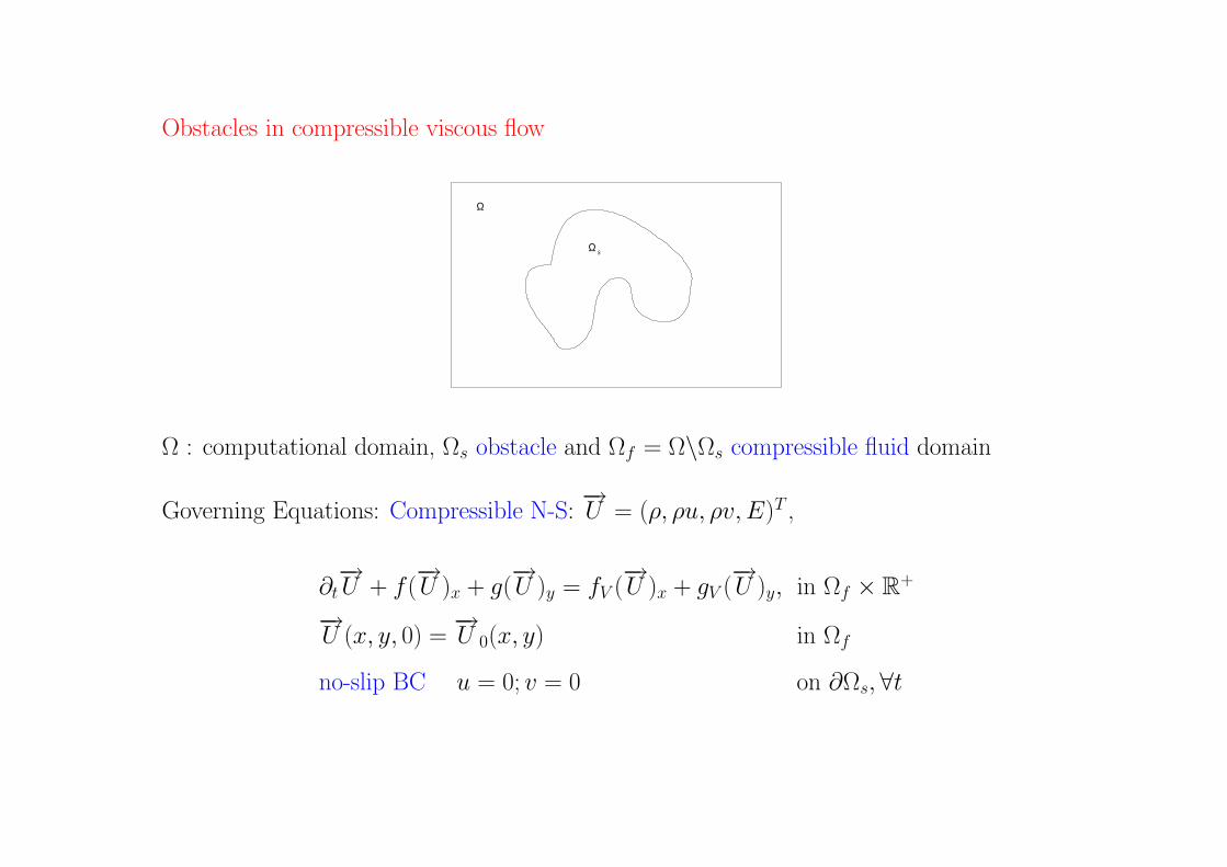
Obstacles in compressible viscous flow
Ω
Ω s
Ω : computational domain, Ωs obstacle and Ωf = Ω\Ωs compressible fluid domain
Governing Equations: Compressible N-S:−→U = (ρ, ρu, ρv, E)T ,
∂t−→U + f(
−→U )x + g(
−→U )y = fV (
−→U )x + gV (
−→U )y, in Ωf × R
+
−→U (x, y, 0) =
−→U 0(x, y) in Ωf
no-slip BC u = 0; v = 0 on ∂Ωs, ∀t
Page 5
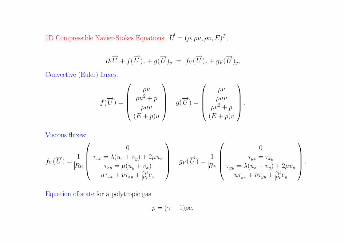
2D Compressible Navier-Stokes Equations:−→U = (ρ, ρu, ρv, E)T ,
∂t−→U + f(
−→U )x + g(
−→U )y = fV (
−→U )x + gV (
−→U )y,
Convective (Euler) fluxes:
f(−→U ) =
ρu
ρu2 + p
ρuv
(E + p)u
g(−→U ) =
ρv
ρuv
ρv2 + p
(E + p)v
.
Viscous fluxes:
fV (−→U ) =
1
Re
0
τxx = λ(ux + vy) + 2µux
τxy = µ(uy + vx)
uτxx + vτxy + γµPr
ex
gV (−→U ) =
1
Re
0
τyx = τxy
τyy = λ(ux + vy) + 2µvy
uτyx + vτyy + γµPr
ey
.
Equation of state for a polytropic gas
p = (γ − 1)ρe.
Page 6
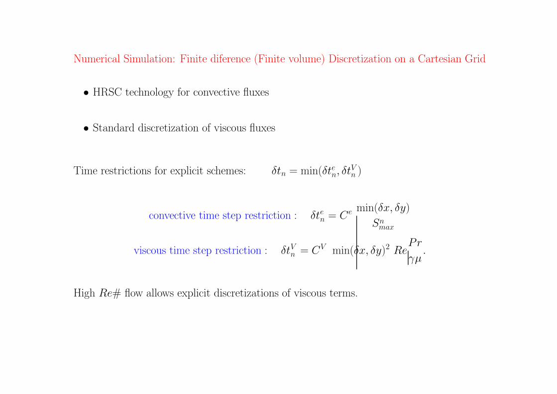
Numerical Simulation: Finite diference (Finite volume) Discretization on a Cartesian Grid
• HRSC technology for convective fluxes
• Standard discretization of viscous fluxes
Time restrictions for explicit schemes: δtn = min(δten, δtVn )
convective time step restriction : δten = Ce min(δx, δy)
Snmax
viscous time step restriction : δtVn = CV min(δx, δy)2 RePr
γµ.
High Re# flow allows explicit discretizations of viscous terms.
Page 7
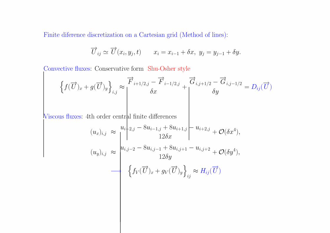
Finite diference discretization on a Cartesian grid (Method of lines):
−→U ij '
−→U (xi, yj, t) xi = xi−1 + δx, yj = yj−1 + δy.
Convective fluxes: Conservative form Shu-Osher style
f(−→U )x + g(
−→U )y
i,j≈
−→F i+1/2,j −
−→F i−1/2,j
δx+
−→G i,j+1/2 −
−→G i,j−1/2
δy= Dij(
−→U )
Viscous fluxes: 4th order central finite differences
(ux)i,j ≈ui−2,j − 8ui−1,j + 8ui+1,j − ui+2,j
12δx+ O(δx4),
(uy)i,j ≈ui,j−2 − 8ui,j−1 + 8ui,j+1 − ui,j+2
12δy+ O(δy4),
−→
fV (−→U )x + gV (
−→U )y
ij≈ Hij(
−→U )
Page 8
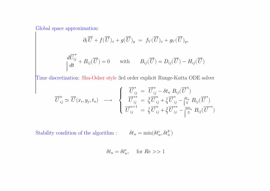
Global space approximation:
∂t−→U + f(
−→U )x + g(
−→U )y = fV (
−→U )x + gV (
−→U )y,
d−→Uij
dt+ Bij(
−→U ) = 0 with Bij(
−→U ) = Dij(
−→U ) − Hij(
−→U )
Time discretization: Shu-Osher style 3rd order explicit Runge-Kutta ODE solver
−→U
n
ij '−→U (xi, yj, tn) −→
−→U
∗
ij =−→U
n
ij − δtn Bij(−→U
n)
−→U
∗∗
ij = 34
−→U
n
ij + 14
−→U
∗
ij −δtn4 Bij(
−→U
∗)
−→U
n+1
ij = 13
−→U
n
ij + 23
−→U
∗∗
ij − 2δtn3 Bij(
−→U
∗∗)
Stability condition of the algorithm : δtn = min(δten, δtVn )
δtn = δten, for Re >> 1
Page 9
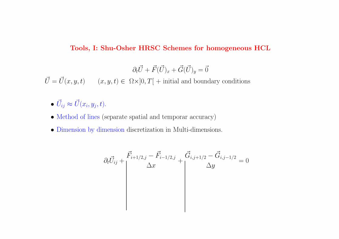
Tools, I: Shu-Osher HRSC Schemes for homogeneous HCL
∂t~U + ~F (~U)x + ~G(~U)y = ~0
~U = ~U (x, y, t) (x, y, t) ∈ Ω×]0, T [ + initial and boundary conditions
• ~Uij ≈ ~U(xi, yj, t).
• Method of lines (separate spatial and temporar accuracy)
• Dimension by dimension discretization in Multi-dimensions.
∂t~Uij +
~Fi+1/2,j − ~Fi−1/2,j
∆x+
~Gi,j+1/2 − ~Gi,j−1/2
∆y= 0
Page 10
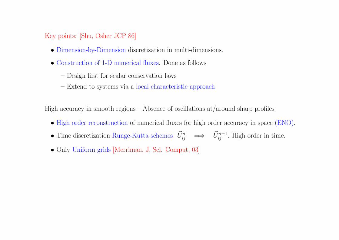
Key points: [Shu, Osher JCP 86]
• Dimension-by-Dimension discretization in multi-dimensions.
• Construction of 1-D numerical fluxes. Done as follows
– Design first for scalar conservation laws
– Extend to systems via a local characteristic approach
High accuracy in smooth regions+ Absence of oscillations at/around sharp profiles
• High order reconstruction of numerical fluxes for high order accuracy in space (ENO).
• Time discretization Runge-Kutta schemes ~Unij =⇒ ~Un+1
ij . High order in time.
• Only Uniform grids [Merriman, J. Sci. Comput, 03]
Page 11
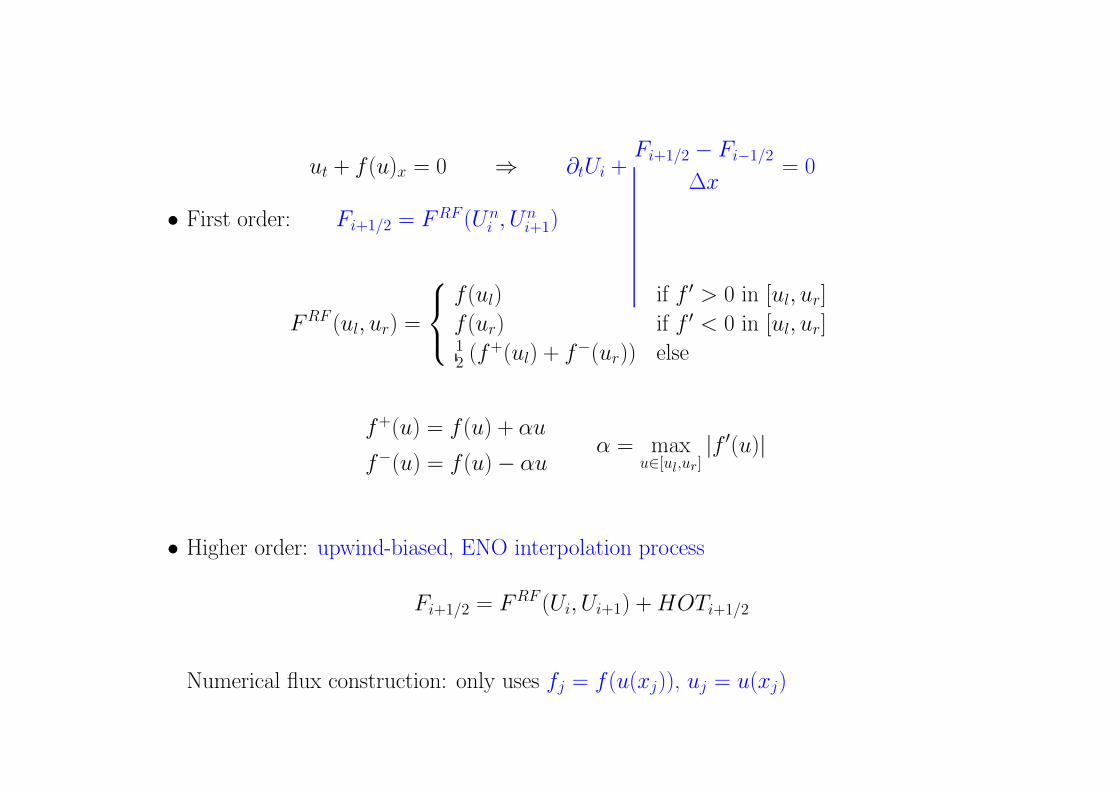
ut + f(u)x = 0 ⇒ ∂tUi +Fi+1/2 − Fi−1/2
∆x= 0
• First order: Fi+1/2 = FRF (Uni , Un
i+1)
FRF (ul, ur) =
f(ul) if f ′ > 0 in [ul, ur]
f(ur) if f ′ < 0 in [ul, ur]12 (f+(ul) + f−(ur)) else
f+(u) = f(u) + αu
f−(u) = f(u) − αuα = max
u∈[ul,ur]|f ′(u)|
• Higher order: upwind-biased, ENO interpolation process
Fi+1/2 = FRF (Ui, Ui+1) + HOTi+1/2
Numerical flux construction: only uses fj = f(u(xj)), uj = u(xj)
Page 12
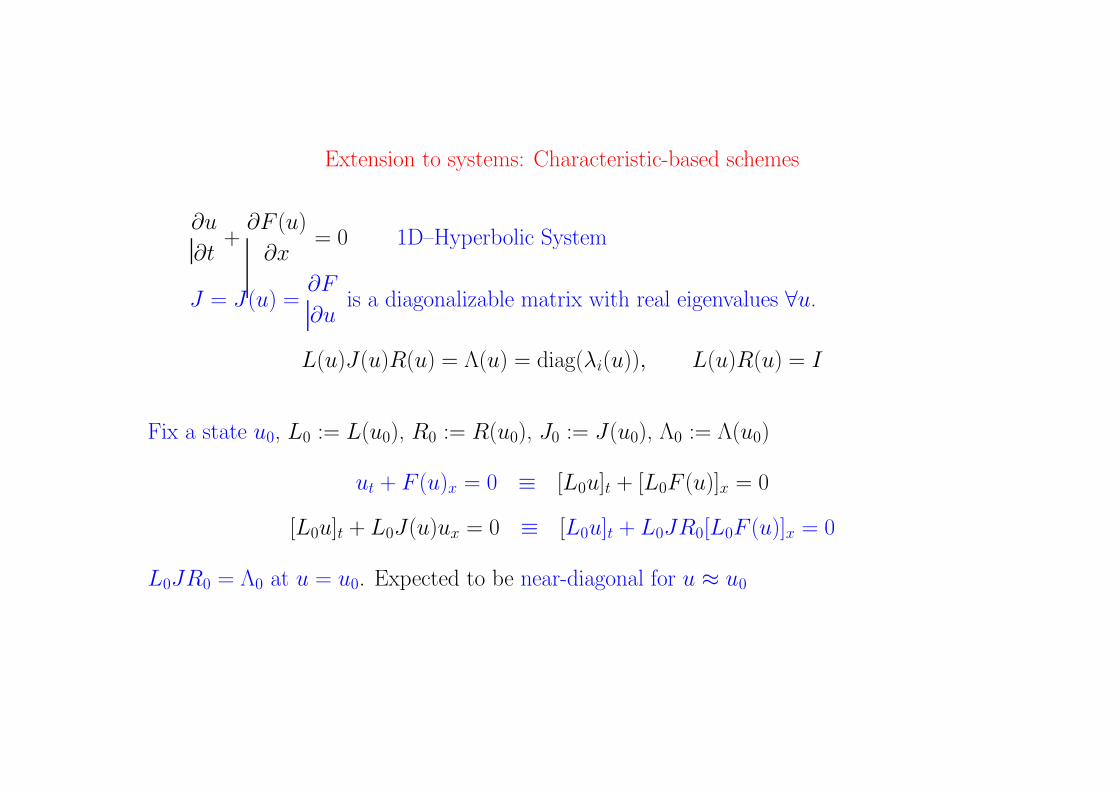
Extension to systems: Characteristic-based schemes
∂u
∂t+
∂F (u)
∂x= 0 1D–Hyperbolic System
J = J(u) =∂F
∂uis a diagonalizable matrix with real eigenvalues ∀u.
L(u)J(u)R(u) = Λ(u) = diag(λi(u)), L(u)R(u) = I
Fix a state u0, L0 := L(u0), R0 := R(u0), J0 := J(u0), Λ0 := Λ(u0)
ut + F (u)x = 0 ≡ [L0u]t + [L0F (u)]x = 0
[L0u]t + L0J(u)ux = 0 ≡ [L0u]t + L0JR0[L0F (u)]x = 0
L0JR0 = Λ0 at u = u0. Expected to be near-diagonal for u ≈ u0
Page 13
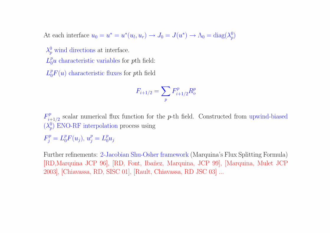
At each interface u0 = u∗ = u∗(ul, ur) → J0 = J(u∗) → Λ0 = diag(λ0p)
λ0p wind directions at interface.
Lp0u characteristic variables for pth field:
Lp0F (u) characteristic fluxes for pth field
Fi+1/2 =∑
p
F pi+1/2R
po
F pi+1/2 scalar numerical flux function for the p-th field. Constructed from upwind-biased
(λ0p) ENO-RF interpolation process using
F pj = Lp
0F (uj), upj = Lp
0uj
Further refinements: 2-Jacobian Shu-Osher framework (Marquina’s Flux Splitting Formula)
[RD,Marquina JCP 96], [RD, Font, Ibanez, Marquina, JCP 99], [Marquina, Mulet JCP
2003], [Chiavassa, RD, SISC 01], [Rault, Chiavassa, RD JSC 03] ...
Page 14
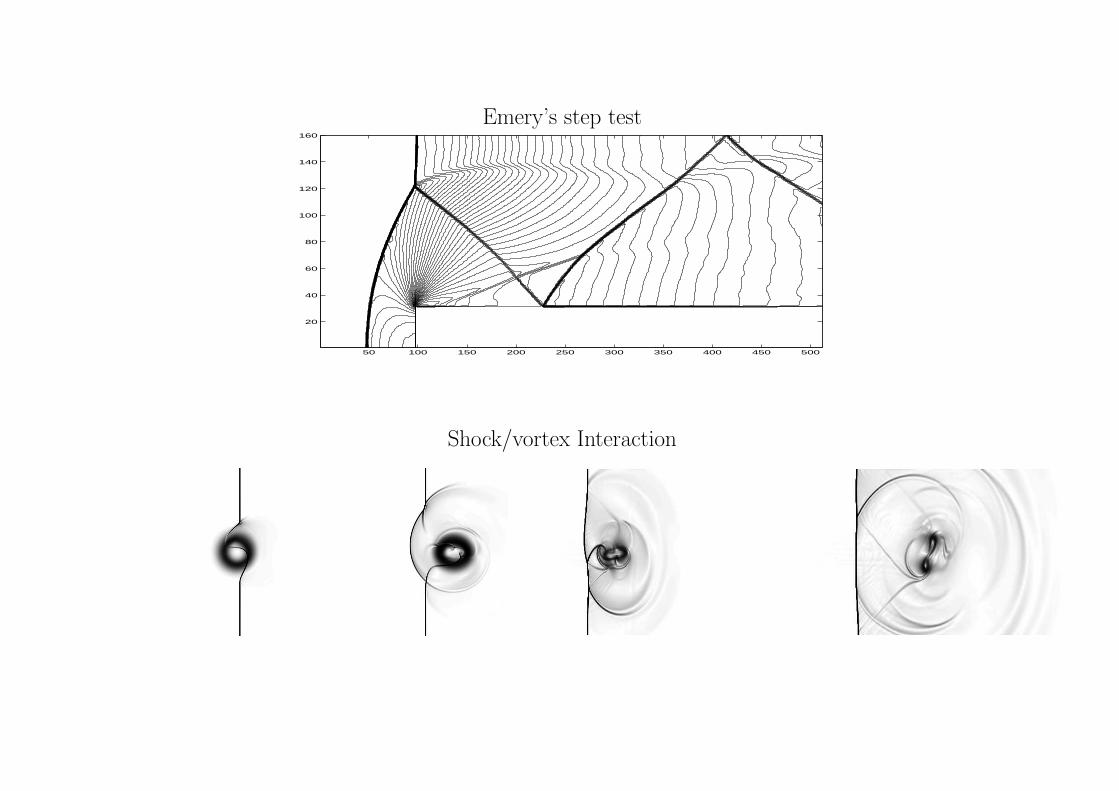
Emery’s step test
50 100 150 200 250 300 350 400 450 500
20
40
60
80
100
120
140
160
Shock/vortex Interaction
Page 15
Tools, II: Penalization methods for obstacles in Incompressible Fluid flow
Goal: Avoid body-fitted unstructured methods in order to use fast/effective spectral, finite-
differences or finite-volume approximations on cartesian meshes.
How: Modify the system of PDEs by adding a penalized velocity term in the momentum
equation
Observation: The penalization has to be extended to the volume of the body to give the
correct physical solutions at high Re.
• Peskin [JCP 77]
• Arquis, Caltagirone [Compt. Rend. A.S.P. 84] Brinkman models with variable perme-
ability for porous media.
• Angot, Bruneau, Fabrie [Num. Math. 99]
Page 16
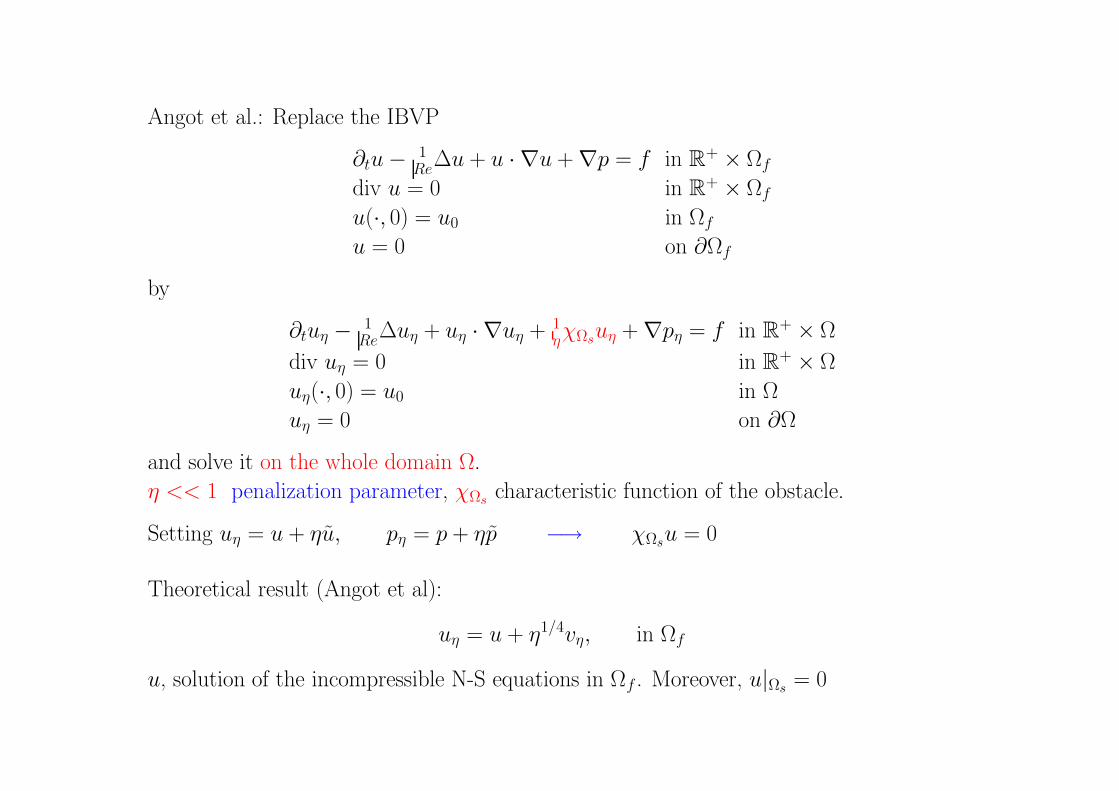
Angot et al.: Replace the IBVP
∂tu − 1Re
∆u + u · ∇u + ∇p = f in R+ × Ωf
div u = 0 in R+ × Ωf
u(·, 0) = u0 in Ωf
u = 0 on ∂Ωf
by
∂tuη −1
Re∆uη + uη · ∇uη + 1
ηχΩsuη + ∇pη = f in R
+ × Ω
div uη = 0 in R+ × Ω
uη(·, 0) = u0 in Ω
uη = 0 on ∂Ω
and solve it on the whole domain Ω.
η << 1 penalization parameter, χΩs characteristic function of the obstacle.
Setting uη = u + ηu, pη = p + ηp −→ χΩsu = 0
Theoretical result (Angot et al):
uη = u + η1/4vη, in Ωf
u, solution of the incompressible N-S equations in Ωf . Moreover, u|Ωs = 0
Page 17
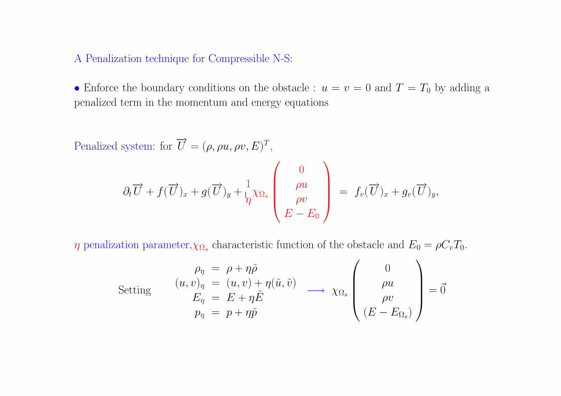
A Penalization technique for Compressible N-S:
• Enforce the boundary conditions on the obstacle : u = v = 0 and T = T0 by adding a
penalized term in the momentum and energy equations
Penalized system: for−→U = (ρ, ρu, ρv, E)T ,
∂t−→U + f(
−→U )x + g(
−→U )y +
1
ηχΩs
0
ρu
ρv
E − E0
= fv(−→U )x + gv(
−→U )y,
η penalization parameter,χΩs characteristic function of the obstacle and E0 = ρCvT0.
Setting
ρη = ρ + ηρ
(u, v)η = (u, v) + η(u, v)
Eη = E + ηE
pη = p + ηp
−→ χΩs
0
ρu
ρv
(E − EΩs)
= ~0
Page 18
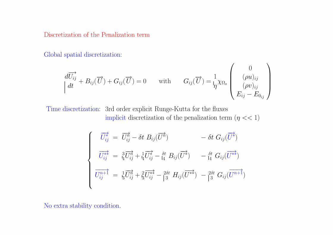
Discretization of the Penalization term
Global spatial discretization:
d−→Uij
dt+ Bij(
−→U ) + Gij(
−→U ) = 0 with Gij(
−→U ) =
1
ηχΩs
0
(ρu)ij(ρv)ij
Eij − E0ij
Time discretization: 3rd order explicit Runge-Kutta for the fluxes
implicit discretization of the penalization term (η << 1)
−→U ∗
ij =−→Un
ij − δt Bij(−→Un) − δt Gij(
−→U ∗)
−→U ∗∗
ij = 34
−→Un
ij + 14
−→U ∗
ij −δt4 Bij(
−→U ∗) − δt
4 Gij(−→U ∗∗)
−−→Un+1
ij = 13
−→Un
ij + 23
−→U ∗∗
ij − 2δt3 Hij(
−→U ∗∗) − 2δt
3 Gij(−−→Un+1)
No extra stability condition.
Page 19
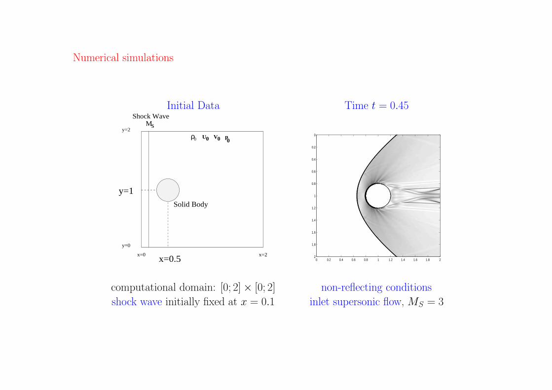
Numerical simulations
Initial Data Time t = 0.45
Solid Body
x=0.5
Shock WavesM
y=1
0p0V0U
y=2
y=0
x=2x=0
0ρ
0 0.2 0.4 0.6 0.8 1 1.2 1.4 1.6 1.8 2
0
0.2
0.4
0.6
0.8
1
1.2
1.4
1.6
1.8
2
computational domain: [0; 2] × [0; 2] non-reflecting conditions
shock wave initially fixed at x = 0.1 inlet supersonic flow, MS = 3
Page 20
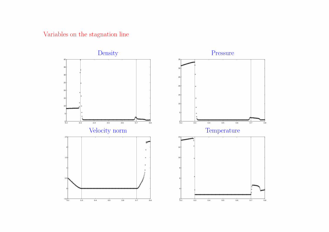
Variables on the stagnation line
Density Pressure
0.2 0.3 0.4 0.5 0.6 0.7 0.80
5
10
15
20
25
30
35
40
0.2 0.3 0.4 0.5 0.6 0.7 0.80
5
10
15
20
25
30
35
Velocity norm Temperature
0.2 0.3 0.4 0.5 0.6 0.7 0.8−0.5
0
0.5
1
1.5
2
2.5
0.2 0.3 0.4 0.5 0.6 0.7 0.82
4
6
8
10
12
14
Page 21
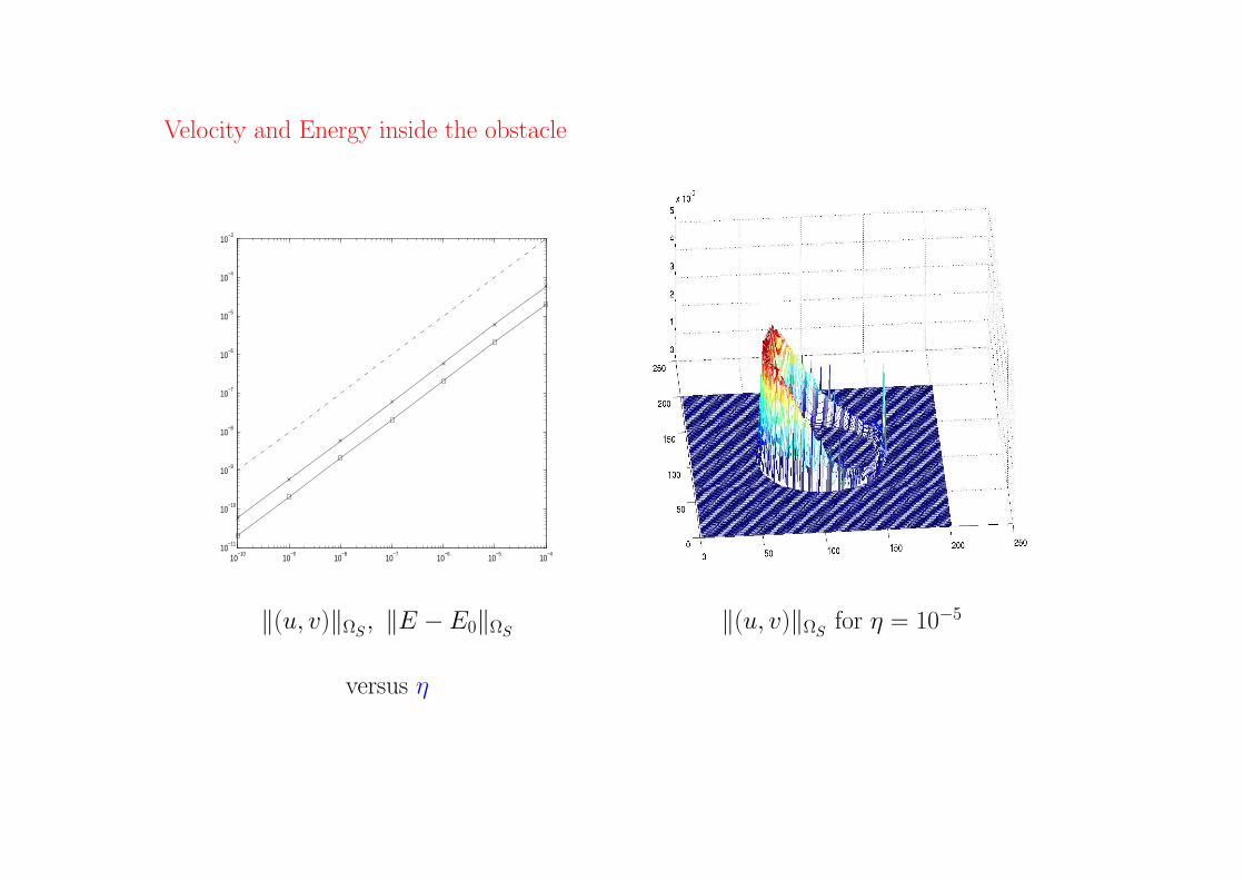
Velocity and Energy inside the obstacle
10−10
10−9
10−8
10−7
10−6
10−5
10−4
10−11
10−10
10−9
10−8
10−7
10−6
10−5
10−4
10−3
‖(u, v)‖ΩS, ‖E − E0‖ΩS
‖(u, v)‖ΩSfor η = 10−5
versus η
Page 22
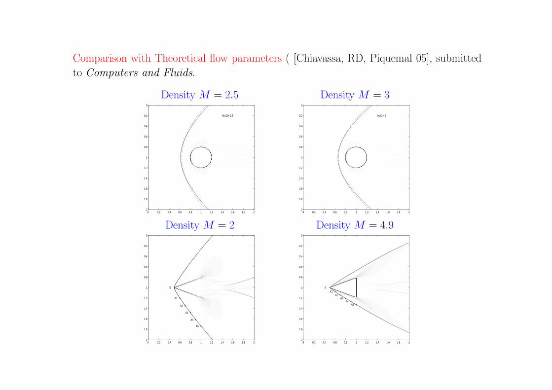
Comparison with Theoretical flow parameters ( [Chiavassa, RD, Piquemal 05], submitted
to Computers and Fluids.
Density M = 2.5 Density M = 3
MACH 2.5
0 0.2 0.4 0.6 0.8 1 1.2 1.4 1.6 1.8 2
0
0.2
0.4
0.6
0.8
1
1.2
1.4
1.6
1.8
2
MACH 3
0 0.2 0.4 0.6 0.8 1 1.2 1.4 1.6 1.8 2
0
0.2
0.4
0.6
0.8
1
1.2
1.4
1.6
1.8
2
Density M = 2 Density M = 4.9
A1
S
A2
A3
A4
A5
0 0.2 0.4 0.6 0.8 1 1.2 1.4 1.6 1.8 2
0
0.2
0.4
0.6
0.8
1
1.2
1.4
1.6
1.8
2
SA1
A2A3
A4A5
0 0.2 0.4 0.6 0.8 1 1.2 1.4 1.6 1.8 2
0
0.2
0.4
0.6
0.8
1
1.2
1.4
1.6
1.8
2
Page 23
Tools, III: Reducing the Computational cost: Multilevel Schemes for HCL
Basic idea:
• Reduce the cost asociated to a HRSC scheme by
reducing the number of costly numerical flux evaluations
• HRSC- Numerical fluxes only needed at/around discontinuities (existing or in formation)
• Analyze the data at each time step of the simulation to determine smoothness zones
HOW?
• Use an appropriate Multiresolution Analysis of the avaliable data.
• Finite Volume formulations: Discrete data are cell-averages
• Shu-Osher Framework: Discrete data are interpreted as point-values
Page 24
MR decompositions of discrete data sets
A multiresolution (MR) decomposition of a discrete data set is an equivalent representation
that encodes the information as a coarse realization of the given data set plus a sequence
of detail coefficients of ascending resolution.
uL → uL−1 → uL−2 → . . . → u0
dL−1 dL−2 . . .d0
uL ≡ MuL = (u0, d1, d2, . . . , dL)
• levels of resolution: Hierarchy of nested computational meshes
• detail coefficients: difference in information between consecutive levels
• direct relation between the detail coefficients and local regularity
Compression properties: Small detail coefficients can be truncated with little loss of
global information contents (Image/signal compression etc..).
Page 25
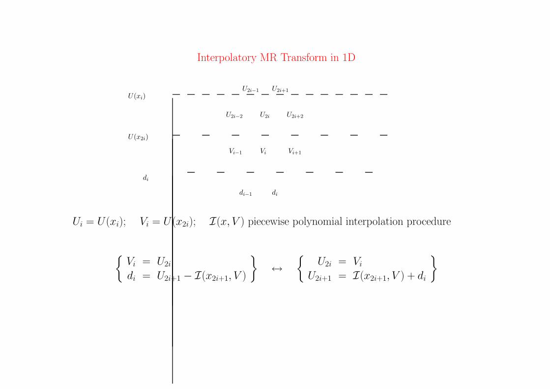
Interpolatory MR Transform in 1D
Vi+1ViVi−1
U2i−2
U2i−1
U2i
U2i+1
U2i+2
di−1 di
U(x2i)
U(xi)
di
Ui = U(xi); Vi = U(x2i); I(x, V ) piecewise polynomial interpolation procedure
Vi = U2i
di = U2i+1 − I(x2i+1, V )
↔
U2i = Vi
U2i+1 = I(x2i+1, V ) + di
Page 26
X l+1
X l
' $v
smooth
?
' $v
?
& %v?
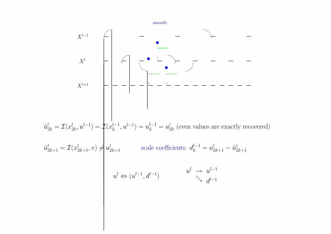
X l−1
ul2k = I(xl
2k, ul−1) = I(xl−1
k , ul−1) = ul−1k = ul
2k (even values are exactly recovered)
ul2k+1 = I(xl
2k+1, v) 6= ul2k+1 scale coefficients: dl−1
k = ul2k+1 − ul
2k+1
ul ⇔ (ul−1, dl−1)ul → ul−1
dl−1
Page 27
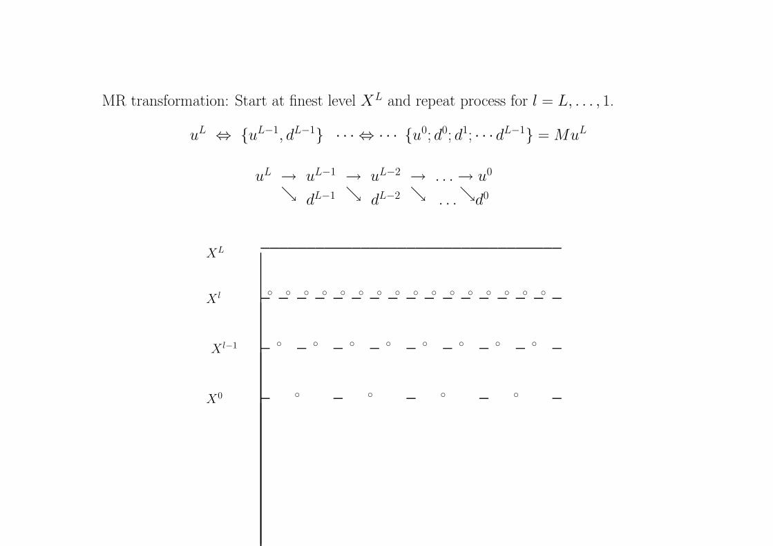
MR transformation: Start at finest level XL and repeat process for l = L, . . . , 1.
uL ⇔ uL−1, dL−1 · · · ⇔ · · · u0; d0; d1; · · · dL−1 = MuL
uL → uL−1 → uL−2 → . . . → u0
dL−1 dL−2 . . .d0
c c c cX0
c c c c c c c cX l−1
c c c c c c c c c c c c c c c cX l
XL
Page 28
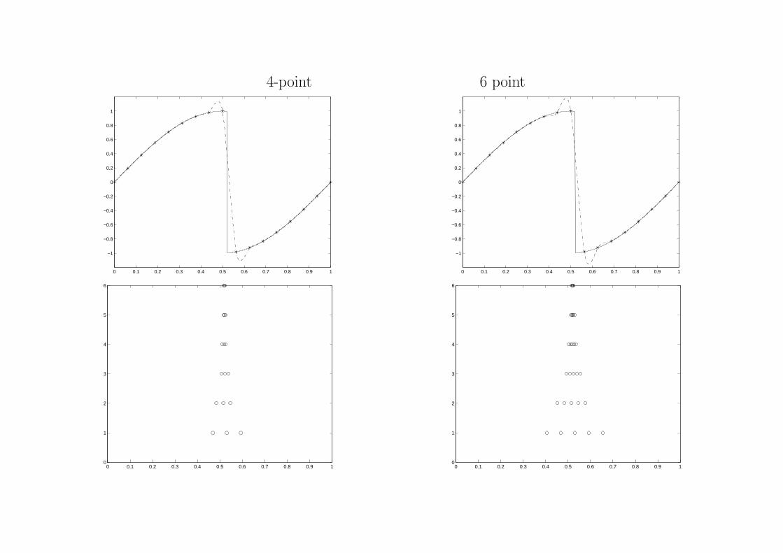
4-point 6 point
0 0.1 0.2 0.3 0.4 0.5 0.6 0.7 0.8 0.9 1
−1
−0.8
−0.6
−0.4
−0.2
0
0.2
0.4
0.6
0.8
1
0 0.1 0.2 0.3 0.4 0.5 0.6 0.7 0.8 0.9 1
−1
−0.8
−0.6
−0.4
−0.2
0
0.2
0.4
0.6
0.8
1
0 0.1 0.2 0.3 0.4 0.5 0.6 0.7 0.8 0.9 10
1
2
3
4
5
6
0 0.1 0.2 0.3 0.4 0.5 0.6 0.7 0.8 0.9 10
1
2
3
4
5
6
Page 29
Adaptive schemes for HCL within Harten’s framework
Numerical values correspond to a particular discretization of the solution.
• Cell-Averages
– Harten (1D)
– Bihari-Harten (2D-tensor product)
– Bihari (1D viscous, source terms, hexahedra)
– Abgrall-Harten (2D-unstructured)
– Dahmen, Gottschlich-Muller, Muller (2D curvilinear)
• Point-Values
– Chiavassa-Donat (2D-tensor product)
Main idea: Exploit the relation between scale coefficents and local regularity of the function
being discretized.
In the interpolatory and cell-average frameworks, the decay rate of the scale coefficients
is related to the smoothness of the data and the order of the interpolation used in the
prediction.
Page 30
• Harten’s original implementation [Comm. Pure and Appl. Math (1995)] seeked to
“Perform a uniform fine grid computation to a prescribed accuracy by reducing
the number of arithmetic operations and computer memory requirements to the
level of an adaptive grid computation”.
• Cost-reduction implementation.
– Bihari-Harten JCP (1996)—SISC (1997) (1D-2D/tensor-product –CA-MR) Bihari
AIAA (2003) (CA-MR unstructured)
– Abgrall-Harten SINUM (1996) (CA-MR unstructured)
– Chiavassa-Donat SISC-(2001) (2D/tensor-product –PV-MR)
– Dahmen, Gottschlich-Muller,Muller Num. Math (2000) (curvilinear meshes, Cell-
Average Framework)
– Cohen, Dyn, Kaber, Postel JCP (2000) (2D-unstructured)
• Fully-Adaptive Implementation.
– Muller(2002); Cohen, Kaber, Muller, Postel (2003) CA linked to an adaptive grid
that evolves in time. Data management required: tree structures (Roussel), hash-
tables (Muller)
Page 31
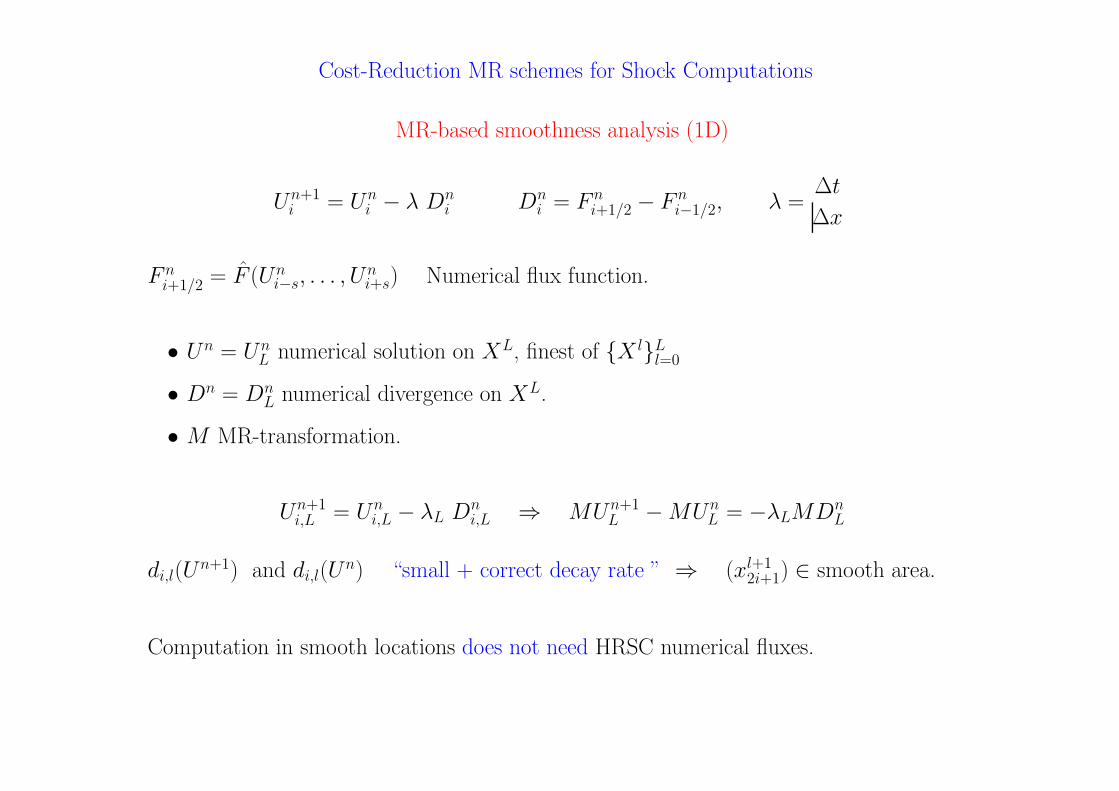
Cost-Reduction MR schemes for Shock Computations
MR-based smoothness analysis (1D)
Un+1i = Un
i − λ Dni Dn
i = F ni+1/2 − F n
i−1/2, λ =∆t
∆x
F ni+1/2 = F (Un
i−s, . . . , Uni+s) Numerical flux function.
• Un = UnL numerical solution on XL, finest of X lL
l=0
• Dn = DnL numerical divergence on XL.
• M MR-transformation.
Un+1i,L = Un
i,L − λL Dni,L ⇒ MUn+1
L − MUnL = −λLMDn
L
di,l(Un+1) and di,l(U
n) “small + correct decay rate ” ⇒ (xl+12i+1) ∈ smooth area.
Computation in smooth locations does not need HRSC numerical fluxes.
Page 32
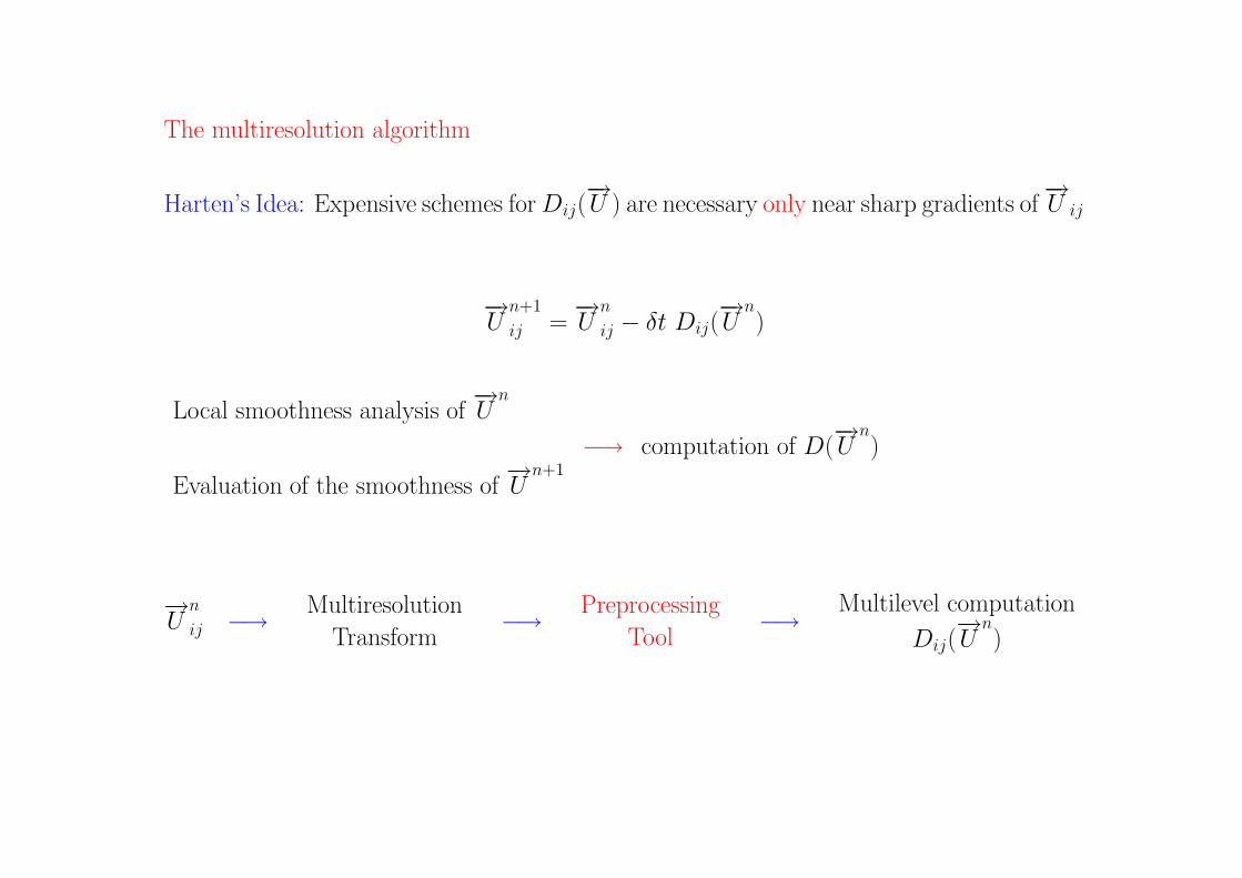
The multiresolution algorithm
Harten’s Idea: Expensive schemes for Dij(−→U ) are necessary only near sharp gradients of
−→U ij
−→U
n+1
ij =−→U
n
ij − δt Dij(−→U
n)
Local smoothness analysis of−→U
n
−→ computation of D(−→U
n)
Evaluation of the smoothness of−→U
n+1
−→U
n
ij −→Multiresolution
Transform−→
Preprocessing
Tool−→
Multilevel computation
Dij(−→U
n)
Page 33
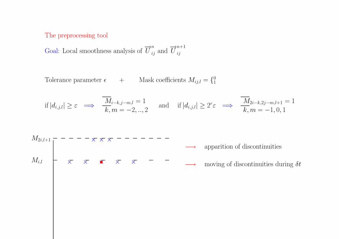
The preprocessing tool
Goal: Local smoothness analysis of−→U
n
ij and−→U
n+1
ij
Tolerance parameter ε + Mask coefficients Mij,l = 01
if |di,j,l| ≥ ε =⇒Mi−k,j−m,l = 1
k, m = −2, .., 2and if |di,j,l| ≥ 2rε =⇒
M2i−k,2j−m,l+1 = 1
k, m = −1, 0, 1
× × × × ×•
× × ×
Mi,l
M2i,l+1
−→ apparition of discontinuities
−→ moving of discontinuities during δt
Page 34
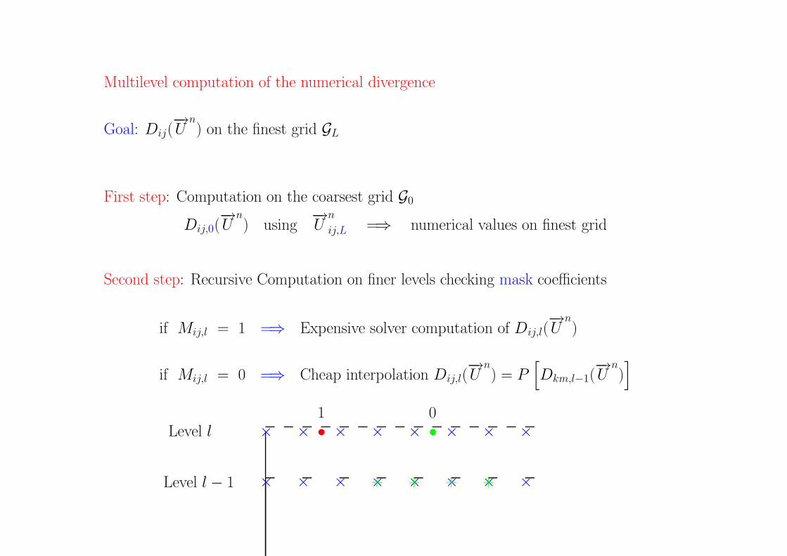
Multilevel computation of the numerical divergence
Goal: Dij(−→U
n) on the finest grid GL
First step: Computation on the coarsest grid G0
Dij,0(−→U
n) using
−→U
n
ij,L =⇒ numerical values on finest grid
Second step: Recursive Computation on finer levels checking mask coefficients
if Mij,l = 1 =⇒ Expensive solver computation of Dij,l(−→U
n)
if Mij,l = 0 =⇒ Cheap interpolation Dij,l(−→U
n) = P
[
Dkm,l−1(−→U
n)]
× × × × × × × ×+ + + +
× × × × × × × ×•1
•0
Level l − 1
Level l
Page 35
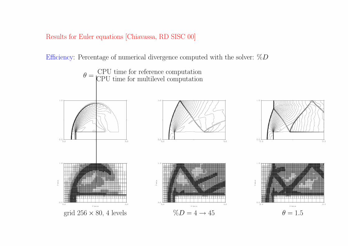
Results for Euler equations [Chiavassa, RD SISC 00]
Efficiency: Percentage of numerical divergence computed with the solver: %D
θ =CPU time for reference computationCPU time for multilevel computation
grid 256 × 80, 4 levels %D = 4 → 45 θ = 1.5
Page 36
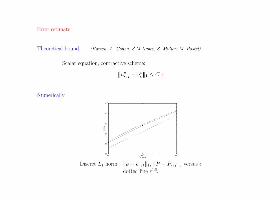
Error estimate
Theoretical bound (Harten, A. Cohen, S.M Kaber, S. Muller, M. Postel)
Scalar equation, contractive scheme:
‖unref − un
ε ‖1 ≤ C ε
Numerically
10−4
10−3
10−2
10−7
10−6
10−5
10−4
10−3
10−2
tolerance ε
erro
r e1
Discret L1 norm : ‖ρ − ρref‖1, ‖P − Pref‖1 versus ε
dotted line ε1.6.
Page 37
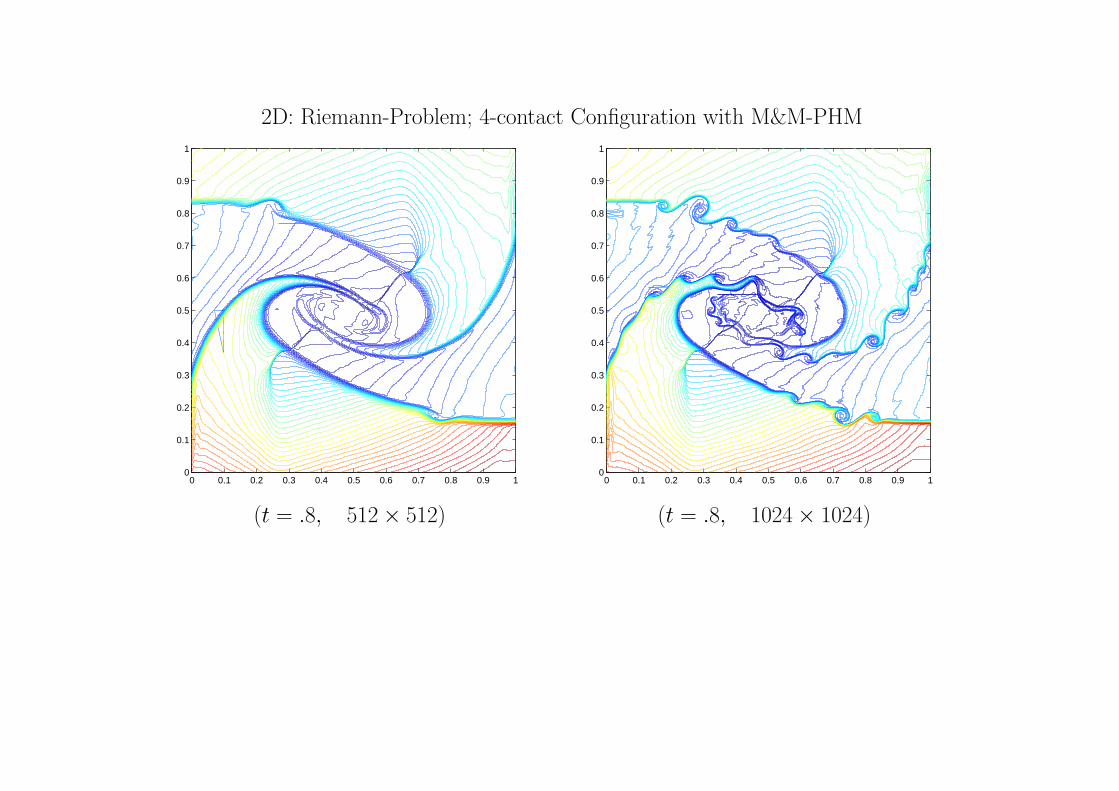
2D: Riemann-Problem; 4-contact Configuration with M&M-PHM
0 0.1 0.2 0.3 0.4 0.5 0.6 0.7 0.8 0.9 10
0.1
0.2
0.3
0.4
0.5
0.6
0.7
0.8
0.9
1
0 0.1 0.2 0.3 0.4 0.5 0.6 0.7 0.8 0.9 10
0.1
0.2
0.3
0.4
0.5
0.6
0.7
0.8
0.9
1
(t = .8, 512 × 512) (t = .8, 1024 × 1024)
Page 38
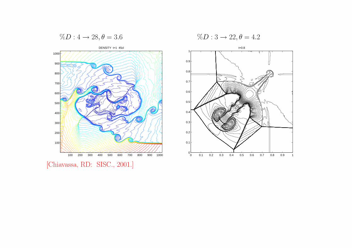
%D : 4 → 28, θ = 3.6 %D : 3 → 22, θ = 4.2
100 200 300 400 500 600 700 800 900 1000
100
200
300
400
500
600
700
800
900
1000
DENSITY t=1 45cl
0 0.1 0.2 0.3 0.4 0.5 0.6 0.7 0.8 0.9 10
0.1
0.2
0.3
0.4
0.5
0.6
0.7
0.8
0.9
1t=0.8
[Chiavassa, RD: SISC., 2001.]
Page 39
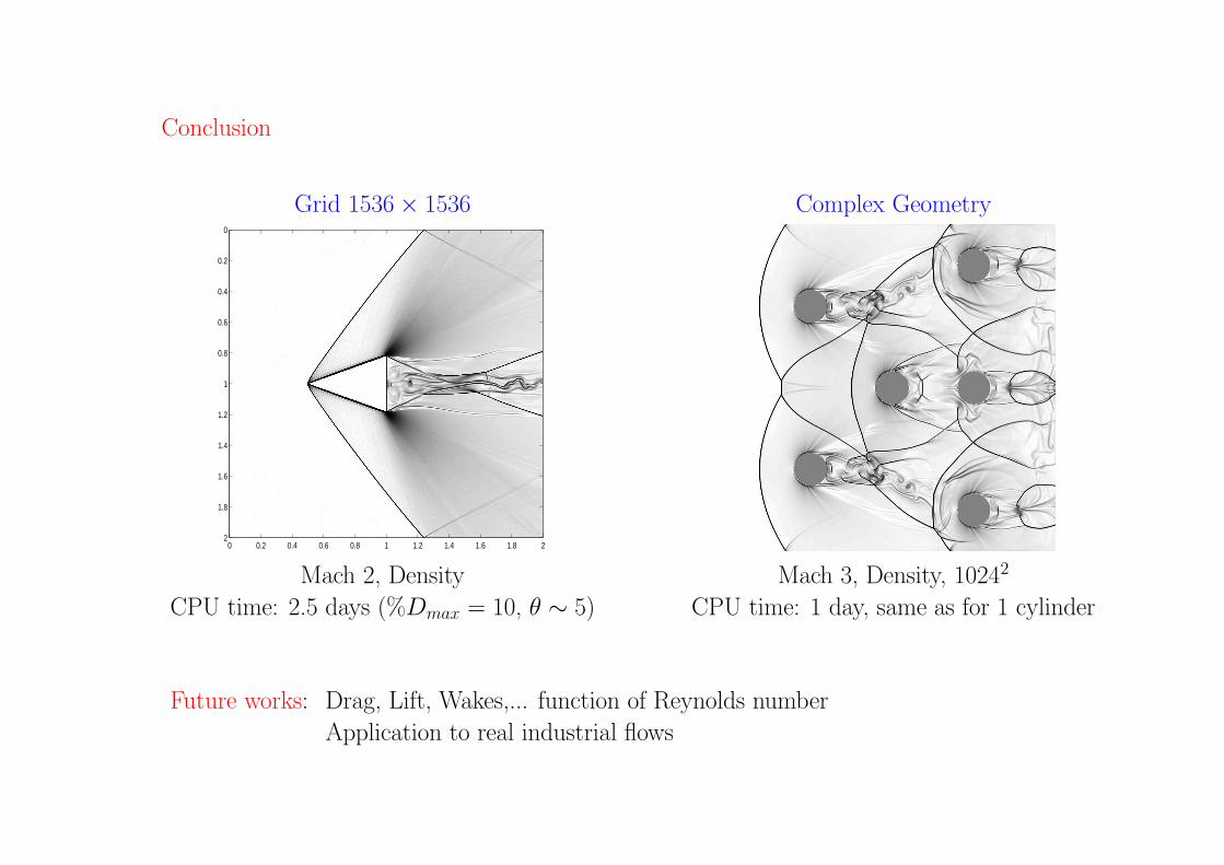
Conclusion
Grid 1536 × 1536 Complex Geometry
0 0.2 0.4 0.6 0.8 1 1.2 1.4 1.6 1.8 2
0
0.2
0.4
0.6
0.8
1
1.2
1.4
1.6
1.8
2
Mach 2, Density Mach 3, Density, 10242
CPU time: 2.5 days (%Dmax = 10, θ ∼ 5) CPU time: 1 day, same as for 1 cylinder
Future works: Drag, Lift, Wakes,... function of Reynolds number
Application to real industrial flows