Published on: Bulletin of Volcanology manuscript No.(will be inserted by the editor)

A Brownian Model for Recurrent Volcanic Eruptions: anApplication to Miyakejima Volcano (Japan)

Alexander Garcia-Aristizabal · Warner Marzocchi ·Eisuke Fujita

Published on: Bulletin of Volcanology (2012) 74:545-558

Abstract The definition of probabilistic models as mathematical structures to describe theresponse of a volcanic system is a plausible approach to characterize the temporal behaviorof volcanic eruptions, and constitutes a tool for long-term eruption forecasting. This kindof approach is motivated by the fact that volcanoes are complex systems in which a com-pletely deterministic description of the processes preceding eruptions is practically impos-sible. To describe recurrent eruptive activity we apply a physically-motivated probabilisticmodel based on the characteristics of the Brownian passage-time (BPT) distribution; thephysical process defining this model can be described by the steady rise of a state variablefrom a ground state to a failure threshold; adding Brownian perturbations to the steady load-ing produces a stochastic load-state process (a Brownian relaxation oscillator) in which aneruption relaxes the load state to begin a new eruptive cycle. The Brownian relaxation os-cillator and Brownian passage-time distribution connect together physical notions of unob-servable loading and failure processes of a point process with observable response statistics.The Brownian passage-time model is parameterized by the mean rate of event occurrence,µ , and the aperiodicity about the mean, α . We apply this model to analyze the eruptive his-tory of Miyakejima volcano, Japan, finding a value of 44.2(±6.5 years) for the µ parameterand 0.51(±0.01) for the (dimensionless) α parameter. The comparison with other modelsoften used in volcanological literature shows that this pysically-motivated model may be agood descriptor of volcanic systems that produce eruptions with a characteristic size. BPTis clearly superior to the exponential distribution and the fit to the data is comparable toother two-parameters models. Nonetheless, being a physically-motivated model, it providesan insight into the macro-mechanical processes driving the system.

A. Garcia-AristizabalIstituto Nazionale di Geofisica e Vulcanologia, via Donato Creti 12, 40128 Bologna, ItalyTel.: +39.051.5141465, Fax: +39.051.4151499E-mail: alexander.garcia@bo.ingv.it

W. MarzocchiIstituto Nazionale di Geofisica e Vulcanologia, Via di Vigna Murata 605, 00143 Roma, Italy

E. FujitaNational Research Institute for Earth Science and Disaster Prevention, Tennodai 3-1, Tsukuba, Ibaraki, 305-0006, Japan

2

Keywords Probabilistic models · Brownian passage-time distribution · Hazard Function ·Miyakejima volcano

PACS PACS 91.40.-k · PACS 91.40.Zz · PACS 91.40.Ft

Mathematics Subject Classification (2000) MSC 86A32 · MSC 60E05 · MSC 62H10

Introduction

Volcanoes can be viewed as complex physical systems in which a completely deterministicdescription of the processes occurring before or during an eruption is practically impossible.This fact motivates the definition and development of probabilistic models as mathematicalstructures to describe physical phenomena: this is a response to the problem in which we donot have direct access to the physical processes, but we can have a record of the responseof the system. In particular, if some characteristic properties of the response of the system(e.g. event times) can be associated with a random variable, and if it is possible to expressa probability function for the random variable, then it is possible to define a probabilisticmodel for the response of the considered system.

A time series of eruptions from a single volcano can be treated as a stochastic point pro-cess with individual eruptions as (random) independent events in time. Statistical analysisof both repose time and erupted volume catalogs have been performed for a large number ofvolcanoes (e.g., Wickman 1976; Klein 1982; Mulargia et al 1985, 1987; De la Cruz-Reyna1991; Burt et al 1994; Marzocchi and Zaccarelli 2006), mainly for those with frequent erup-tive activity and where detailed catalogs exist. The main objective of this kind of analysis isto develop probabilistic models to understand the past eruptive activity of the volcano andto forecast its future behavior.

When treating eruptions as events in time, several simplifying assumptions must be made(Klein 1982; Ho 1991): although the onset date of an eruption is generally well constrained,the duration some times is harder to determine and/or is rarely reported. In our analysis, weignore eruption duration since we take the onset date as the most physically meaningful,and measure repose times from one onset date (of an eruptive episode) to the next. In thisway, our modeling intends to describe the waiting times of the long-term physical processesgoverning renewed volcanic activity. Once the volcanic system has been perturbed and anew eruptive episode has started, the short-term behavior of the eruptive activity may followdifferent patterns during the gradual decline of activity; in this context, sporadic eruptiveactivity in a short time window (with respect to the repose time) after the onset of a neweruptive episode cannot be described using the former long-term model. Thus, the definitionof repose time from this point of view is not exactly equivalent to the classic concept ofnon-eruptive period; this assumption seems justified because most eruption durations aremuch shorter than typical effective repose intervals (e.g., Klein 1982).

Some distinct conceptual models have been proposed to describe the eruptive behavior ofdifferent volcanoes around the world. The most frequent solutions describe the eruptiveactivity in terms of (1) a homogeneous Poisson processes in the time domain (e.g., Klein1982; De la Cruz-Reyna 1991; Marzocchi and Zaccarelli 2006), (2) Time-Predictable pro-cesses (e.g., Burt et al 1994; Sandri et al 2005; Marzocchi and Zaccarelli 2006) or (3) Size-Predictable processes (e.g., Burt et al 1994; Marzocchi and Zaccarelli 2006). In our analy-

3

sis, none of these existing models successfully explains the eruptive activity of Miyakejimavolcano, which seems to show a more regular behavior and a characteristic size for theerupted volumes. Other probabilistic models often used in literature were also tested, asfor example the Loglogistic process (e.g., Connor et al 2003; Watt et al 2007), and a non-homogeneous Poisson process modeled using a Weibull process (e.g., Ho 1991; Bebbingtonand Lai 1996a,b). In this paper we present an interesting, physically-motivated, probabilisticmodel based on the Brownian passage-time distribution which has not been used before forvolcanological problems; we apply it to analyze the time series of repose times (as defined),τ , of Miyakejima volcano, and compare its performance respect to other models often usedin volcanology.

The Models

Most of the models considered here are based on generic distributions that characterizerenewal processes that in general may have some physical meaning and applicability. A re-newal process has the property that the inter-occurrence times are independent and identically-distributed, positive, random variables having a common distribution F(τ). We have alsoconsidered for test two non-renewal processes: the size-predictable (SPM) and the time-predictable (TPM) models.

Brownian Passage-Time Model (BPT)

A particularly interesting renewal model is the Brownian passage-time model (BPT). It wasoriginally introduced by Matthews et al (2002) and Ellsworth et al (1999) to provide aphysically-motivated renewal model for earthquake recurrence. It is based on the propertiesof the Brownian relaxation oscillator (BRO). A BPT model considers an event (earthquakesin Matthews’ model or renewed eruptive activity in our case) as a realization of a pointprocess in which new eruptive activity will occur when a state variable (or a set of them)reaches a threshold (X f ) and at which time the state variable returns to a base ground level(X0). Adding Brownian perturbations to steady loading of the state variable X produces astochastic load-state process. An eruption relaxes the load state to the characteristic groundlevel and begins a new cycle. The load-state process is a BRO, while intervals betweenevents have a distribution known as Brownian passage-time distribution. Note that this isthe name used in physics literature; in the statistics literature it is often known as InverseGaussian or Wald distribution (Matthews et al 2002).

In the conceptual model of Matthews et al (2002), the loading of the system has two com-ponents: (1) a constant-rate loading component, λ t, and (2) a random component, ε(t) =σW (t), that is defined as a Brownian motion (where W is a standard Brownian motion andσ is a non-negative scale parameter). Standard Brownian motion is simply integrated sta-tionary increments where the distribution of the increments is Gaussian (which might bemotivated by central-limit arguments if we consider perturbations as the sum of many small,independent contributions), with zero mean and constant variance. The Brownian perturba-tion process for the state variable X(t) (see figure 2 in Matthews et al (2002)) is defined as:

X(t) = λ t +σW (t) (1)

4

An event will occur when X(t)≥ X f ; event times are seen as “first passage” times of Brow-nian motion with drift (Matthews et al 2002), which means that eruptive episodes take placewhen the threshold X f is first reached. The BRO are a family of stochastic renewal pro-cesses defined by four parameters: the drift or mean loading (λ ), the perturbation rate (σ2),the ground state (X0), and the failure state (X f ). On the other hand, the recurrence propertiesof the BRO (repose times) are described by a Brownian passage-time distribution which ischaracterized by two parameters: (1) the mean time or period between events, (µ), and (2)the aperiodicity of the mean time, α , which is equivalent to the familiar coefficient of vari-ation (defined in equation 3). The probability density for the BPT model is given by:

f (t; µ;α) =( µ

2πα2t3

) 12 e

{− (t−µ)2

2α2µt

}(2)

The state variable X(t) is a formal parameter of a point process model and represents aconstant-rate mean path that embodies a macroscopic view of a uniform loading of thevolcanic system. It may summarize the macro-mechanics of the volcanic system controlledby one or more physical variables. An explicit definition of the driving physical parametersmay be unrealistic and impossible to demonstrate from our analysis. Independently of itsphysical nature, the state variable should be a parameter that accumulates with time duringrepose episodes, up to a critical value beyond which the system becomes perturbed enoughand a new eruptive process may be triggered. Then, the eruptive process relaxes the systemand the state variable returns to a ground level and a new cycle starts. The perturbationfactor ε(t) represents the total sum of all other factors which may play a role in the recurrenteruptive process considered and/or that may randomly disturb the state variable producingthe aperiodicity of the mean time between eruptions (e.g. effects from tectonic environment,changes in the magma rate supply, compositional changes).

Other models often used in volcanological problems

Poisson Process in the time domain: random model of eruption occurrences

The Poisson process is an important model often used to describe the patterns of eruptionoccurrences in volcanoes (e.g., Klein 1982; Mulargia et al 1985). It is mainly applicable tomajor eruptive activity involving a significant release of mass and energy (De la Cruz-Reyna1991). In a Poisson process the repose times follow an Exponential distribution. It charac-terizes a random volcano, which is one that is ready to erupt at any time. An alternativepossibility is that the eruption sequence is periodic to some degree, and that a certain reposetime is favored; if eruptions were periodic, the distribution of repose times would be peakedinstead of containing an exponentially decreasing number of larger times, as predicted bythe Exponential model. In order to explore the degree of departure from a homogeneousPoisson process, we calculate the coefficient of variation, η , given by

η =σµτ

(3)

where µτ and σ are, respectively, the average and standard deviation of the repose times τ(Marzocchi and Zaccarelli 2006). The coefficient η may help us to quantify if and how muchthe statistical distribution of τ differs from a Poisson process: for a Poisson process (and thenan Exponential distribution of τ), η = 1; more clustered distributions have η > 1 and formore regular recurrent times η < 1 (e.g., Cox and Lewis 1966; Marzocchi and Zaccarelli2006).

5

Renewal models described by Weibull, Gamma, Lognormal and Loglogistic distributions

In renewal models, the random variable τ represents the lifetime or time to failure of a sys-tem. To analyze the intrinsic characteristics of this kind of probabilistic models, it is oftenmore informative to consider the hazard function (also known as hazard rate, or intensityfunction) of the model than to look at the shape of the Probability Density Function (PDF)or Cumulative Distribution Function (CDF) directly; for this reason we make extensive useof the hazard function to compare the different renewal models considered. The hazard func-tion describes the instantaneous failure rate, or the conditional density of failure at a giventime, considering the information that no event occurred until that time. A more detaileddescription of the hazard function concept can be found forward in this paper.

The Exponential distribution (and its implicit homogeneous Poisson process) has a con-stant hazard function, highlighting its characteristic no-memory property. However, whenprocesses like wearing, improvement, learning and growth are implicit in the physical sys-tem, then it is necessary to consider models where the hazard function must be a functionof time. The Weibull, Gamma, Lognormal and Inverse Gaussian (the last one is described inthe next section) are the models with those characteristics that are widely used in the litera-ture.

The Weibull is one of the models most used in volcanological applications (e.g., Ho 1991,1996; Bebbington and Lai 1996a,b). The Weibull process (WEI(ν ,θ )) is one of the possiblegeneralizations of the Exponential case; θ and ν may be interpreted, respectively, as the de-gree of clustering/periodicity and the underlying activity (e.g., Bebbington and Lai 1996a).If the volcanism is waning or developing, the model is generalized to allow the rate of vol-canic events (which is constant in the homogeneous case) to be a decreasing or increasingfunction of time (Ho 1996). This can be defined as a non-homogeneous Poisson process(Bain 1978). The Gamma distribution (GAM(ν ,θ )) provides an alternative generalization ofthe Exponential distribution but with different characteristics with respect to the Weibull; infact, if we consider the hazard function for the Gamma model, the event rate may increaseinitially, but after some time the system would reach a stable condition and then it tends to aconstant hazard rate (Bain 1978). This is considerably different in the Weibull model where,for θ > 1, the hazard function tends to infinity as the time tends to infinity. The Lognormalmodel has been considered for periodicity tests by some authors (e.g., Bebbington and Lai1996a). In this case, the hazard function has a similar behavior as the Gamma model but withthe difference that the asymptotic event-rate goes to zero as the time goes to infinity. Finally,we also consider the possibility of a Loglogistic model, characterized by two parameters: µ ,a location parameter, and σ , a scale parameter, which has been used by some authors (e.g.,Connor et al 2003; Watt et al 2007) to successfully describe data in some volcanologicalapplications.

Time predictable (TPM) and Size predictable (SPM) models

TPM and SPM are widely used in both seismological and volcanological literature. Both ofthem imply a functional relationship between size (of eruptions) and repose times. In thecase of TPM, the time to the next eruption depends on the time required for magma enteringthe storage system to reach the eruptive level (Burt et al 1994). It can be described using ageneral definition of the form τi ∝ [Vi]

β , where ∝ stands for ’proportional to’ (Sandri et al

6

2005). A reliable application of a TPM requires that the size (e.g. erupted volume, explosiv-ity index, etc.) of the eruptions has to be significantly correlated to the logarithm of the timeto the next eruption (Marzocchi and Zaccarelli 2006). The applicability of this model relieson two main assumptions: (1) eruptions occur when a threshold of the magma volume in thestorage system is reached, and (2) the magma input in the storage system is a well definedfunction of the reservoir to be filled to reach that threshold; the specific case of β = 1 meansthat the input rate is constant (Marzocchi and Zaccarelli 2006).

On the other hand, in a SPM the duration of the repose time of the volcano (i.e. the timesince the last eruption) is the parameter which is useful to forecast the size of the nexteruption. As for the TPM case, the most general functional relationship between volumesand repose times for a SPM is of the form Vi ∝ τβ

i (e.g., Marzocchi and Zaccarelli 2006).In this case, the model relies on two main assumptions: (1) the output of each eruption isdetermined only by the magma accumulated since the last eruption, and (2) as in the previ-ous case, the magma enters in the plumbing system at a rate described by a ’well defined’function of the magma volume in the reservoir.

Miyakejima volcano and data set

Miyakejima volcano

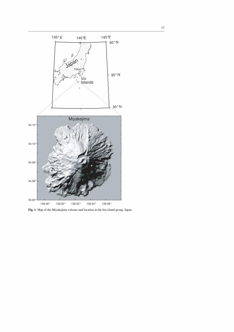
Miyakejima island, located about 200 km south of Tokyo (Fig. 1), is one of the most activebasaltic volcanoes in Japan. Its recurrent eruptive behavior has been observed but up to nowa detailed quantitative analysis based on its past activity has not been performed. In mosthistorical eruptions, basaltic lava and scoria erupted mainly from flank fissures (Tsukui andSuzuki 1998) and most eruptions lasted a short time (a day to a month). The latest eruptiveepisode started in June 2000 and a caldera formed at the summit; since then, the volcanohas been showing some seismic swarms accompanied by important gas emissions for morethan 9 years. On the basis of surface phenomena observed, many authors divided the 2000-2010 eruptive period into at least four stages (e.g., Nakada et al 2005; Ueda et al 2005):(1) magmatic intrusion (1 day), (2) summit subsidence (10 days), (3) Explosion (40 days),and (4) gas emissions accompanied by small seismic swarms, deformation and explosions(>9 years). The total volume of tephra erupted was about 0.009 km3 (DRE), which is muchsmaller than the volume of the resulting caldera (0.6 km3) (Nakada et al 2005).

(FIGURE 1 (MAP OF MIYAKEJIMA...) SOMEWHERE AROUND HERE)

Here we analyze a data set containing the repose periods and volumes of lava and tephraemitted by Miyakejima volcano based on the historical data published by Tsukui and Suzuki(1998) and from the Global Volcanism Program catalog (Simkin and Siebert 2002 onwards).The data set was updated introducing information of the last eruption (June 2000) fromNakada et al (2005) (Table 1).

Data set of eruptions and completeness of the catalog

In order to extract unbiased information from a catalog it is necessary to check for its com-pleteness. This issue is well known in seismology where the completeness of catalogs is

7

Table 1 Summary of the eruptive history of Miyakejima (this table updates the catalog provided by Tsukuiand Suzuki (1998). The volume of the 2000 eruption is from Nakada et al (2005); some dates missing inTsukui and Suzuki (1998) are from the Global Volcanism Program (Simkin and Siebert 2002 onwards). TheVEI values are calculated based on the DRE volumes using the criteria defined by Newhall and Self (1982).Eruption numbers accompanied by (∗) mark are those considered in the present study (after the completenessanalysis).

Num. Kind Date DRE volume (km3) VEI

29∗ 2000 Scoria 2000 Jun 27 (AD) 0.009 328∗ 1983 Scoria + Lava 1983 Oct 03 (AD) 0.007 227∗ 1962 Scoria + Lava 1962 Aug 24 (AD) 0.006 226∗ 1940 Scoria + Lava 1940 Jul 12 (AD) 0.015 325∗ 1874 Scoria + Lava 1874 Jul 03 (AD) 0.010 324∗ 1835 Lava 1835 Nov 11 (AD) <0.001 <223∗ 1811 Scoria 1811 Jan 27 (AD) <<0.010 2

1769 (?) Lava 0.00122∗ 1763 (?) Lava 1763 Aug 17 (AD) 0.001 3

Shinmio Explosion Breccia (SMB) 0.0311763 Scoria 0.033

21∗ 1712 Lava 1712 Feb 04 (AD) 0.001 220∗ 1643 Scoria 1643 Mar 31 (AD) 0.009 3

1643 Lava 0.00319∗ Kamakata Lava (KKL) 1595 Nov 22 (AD) <0.001 <218∗ Benkenezaki Lava (BKL) 1535 Mar (AD) 0.003 217∗ Enokizawa Lava (EZL) 1469 Dec 24 (AD) 0.002 216 Son-ei Bokujo Ash (SBA) 1154 AD (?) 0.040 3

1154 Scoria <<0.01015 Nanto Lava (NTL) 1085 AD (?) 0.012 2

Kamane Scoria (KMS) 10-11C AD (?) 0.01014 Miike Explosion Breccia (MKB) 838-886 AD 0.040 3

Oyama Scoria 0.030Oyama Lava 0.012

13 Kazahaya Scoria (KHS) 832 AD 0.007 212 Mitoribata Scoria (MBS) 1290 yBP 0.007 211 Daihannya-yama Scoria (DHS) 500 AD 0.010 3

Anegakata Lava 0.00110 Sabigahama Explosion Breccia (SHB) 320 AD (?)<0.010 2

Togahama-south Lava (TSL) <0.0019 Togataira Ash (TGA) 260 AD 0.040 3

Togataira Scoria (TGS) 0.005Usuki-west Scoria (UWS) n.dIgayazawa Scoria 0.010

8 Tairayama Lava (TYL) 2050 yBP 0.001 3Tairayama Scoria (TYS) 0.020

7 Izu Scoria (IZS) 600 BC 0.050 36 Hatchodaira Accrtionary Lapilli (HCA) 2500-3000 yBP 0.200 4

Furumio Explosion Breccia (FMB)Hatchodaira Scoria (HCS) 0.170Nagane Scoria (NGS) 1450 BC n.d.

5 Tsubota Scoria (TBS) 3000 yBP(?) 0.010 24 Mizutamari Explosion Breccia (MZB) 3500 yBP(?) 0.062 33 Igaya-east Scoria (IES) 3660 yBP <<0.010 22 Igaya Accrtionary Lapilli (IGA) 4000 yBP 0.090 3

Izushita Lava (ISL) (?)0.0011 Ofunato Explosion Breccia (OFB) 7000-8000 yBP 0.150 4

8

often checked by analyzing the Gutenberg-Richter law and/or the time evolution of the rateof occurrence of events. In volcanology however, the incompleteness of a catalog of erup-tions may be more difficult to evaluate because there are only weak indications that a generalpower law applies (Simkin and Siebert 2002 onwards), and also because we know that vol-canoes may have different eruptive regimes in their history and then the eruptive rate maychange with time (e.g., Ho 1991; Marzocchi and Zaccarelli 2006; Coles and Sparks 2006).Because of this difficulty, when we talk about the completeness of a given eruptive sequence,we understand it as a period of “uniformity” in the data set.

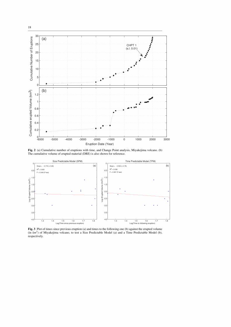
To analyze the completeness of the catalog we plot the cumulative number of eruptions intime, as seen in Figure 2a, and identify changes in the statistics of the repose times. Changesin the statistics of the sequence are identified applying a change point strategy (CHPT). Thechange point hunting methods aim to find one or more statistically significant change pointsin a sequence of data. Here we use a method based on the two-sample Kolmogorov-Smirnovstatistics (a non-parametric test for equal distributions), which has been proposed and testedby Mulargia and Tinti (1985) and Mulargia et al (1987).

(FIGURE 2 (CUMULATIVE NUMBER OF ERUPTIONS...) SOMEWHERE AROUNDHERE)

The cumulative plot in Fig. 2a shows a curve with a slope changing with time. Changesin the slope may be due to different factors as changes in the eruptive regime and/or under-reporting of eruptions in past time (incompleteness of the catalog). Applying the CHPTstrategy, we identify one change point (with 0.01 significance level threshold) between theeruptions 16 and 17 of the catalog (1154 and 1469 AD respectively, see table 1). It meansthat we can consider the catalog to be “uniform” in the period from 1469 up to now (13eruptive episodes), and then our analysis is oriented to describe the eruptive regime of thevolcano within this period. It is important to remark that volcanoes may change eruptiveregime through time: our analysis and the derived eruption forecasting assessment is basedon the eruptive regime shown by the volcano in the last (around) 540 years, and is valid onlyunder the assumption that in the future it will behave in the same way.

Data Analysis and Results

Our analysis consists of four groups of tests which can be summarized as: (1) test of a SPMand a TPM; (2) test of a homogeneous Poisson process in the time domain, (3) tests ofthe Brownian passage-time model, and (4) test of other possible renewal models describingdifferent processes (e.g. recurrent, non-homogeneous Poisson); in this case we have consid-ered as possible candidate distributions four models often used in volcanology: Lognormal,Gamma, Weibull, and Log-logistic.

We estimate the model parameters for each candidate model using a Maximum LikelihoodEstimate (MLE) approach, and use the Akaike Information criteria (AIC, Akaike 1974) forthe model selection; the AIC is a tool based on the concept of entropy, and offers a rel-ative measure of the information lost when a given model is used to describe some data(a trade-off between accuracy and complexity of the model). On the other hand, SPM andTPM models are tested by regression analysis of repose times and sizes (erupted volumesand VEI).

9

Estimating the parameters of the considered models

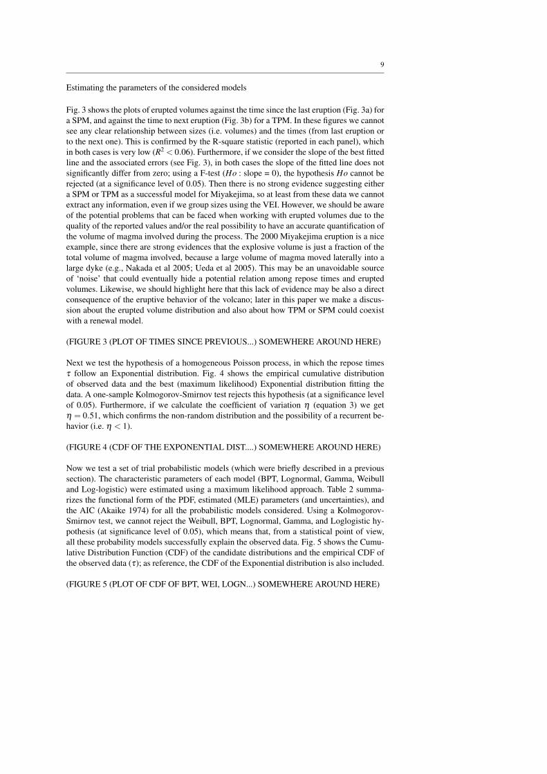
Fig. 3 shows the plots of erupted volumes against the time since the last eruption (Fig. 3a) fora SPM, and against the time to next eruption (Fig. 3b) for a TPM. In these figures we cannotsee any clear relationship between sizes (i.e. volumes) and the times (from last eruption orto the next one). This is confirmed by the R-square statistic (reported in each panel), whichin both cases is very low (R2 < 0.06). Furthermore, if we consider the slope of the best fittedline and the associated errors (see Fig. 3), in both cases the slope of the fitted line does notsignificantly differ from zero; using a F-test (Ho : slope = 0), the hypothesis Ho cannot berejected (at a significance level of 0.05). Then there is no strong evidence suggesting eithera SPM or TPM as a successful model for Miyakejima, so at least from these data we cannotextract any information, even if we group sizes using the VEI. However, we should be awareof the potential problems that can be faced when working with erupted volumes due to thequality of the reported values and/or the real possibility to have an accurate quantification ofthe volume of magma involved during the process. The 2000 Miyakejima eruption is a niceexample, since there are strong evidences that the explosive volume is just a fraction of thetotal volume of magma involved, because a large volume of magma moved laterally into alarge dyke (e.g., Nakada et al 2005; Ueda et al 2005). This may be an unavoidable sourceof ‘noise’ that could eventually hide a potential relation among repose times and eruptedvolumes. Likewise, we should highlight here that this lack of evidence may be also a directconsequence of the eruptive behavior of the volcano; later in this paper we make a discus-sion about the erupted volume distribution and also about how TPM or SPM could coexistwith a renewal model.

(FIGURE 3 (PLOT OF TIMES SINCE PREVIOUS...) SOMEWHERE AROUND HERE)

Next we test the hypothesis of a homogeneous Poisson process, in which the repose timesτ follow an Exponential distribution. Fig. 4 shows the empirical cumulative distributionof observed data and the best (maximum likelihood) Exponential distribution fitting thedata. A one-sample Kolmogorov-Smirnov test rejects this hypothesis (at a significance levelof 0.05). Furthermore, if we calculate the coefficient of variation η (equation 3) we getη = 0.51, which confirms the non-random distribution and the possibility of a recurrent be-havior (i.e. η < 1).

(FIGURE 4 (CDF OF THE EXPONENTIAL DIST....) SOMEWHERE AROUND HERE)

Now we test a set of trial probabilistic models (which were briefly described in a previoussection). The characteristic parameters of each model (BPT, Lognormal, Gamma, Weibulland Log-logistic) were estimated using a maximum likelihood approach. Table 2 summa-rizes the functional form of the PDF, estimated (MLE) parameters (and uncertainties), andthe AIC (Akaike 1974) for all the probabilistic models considered. Using a Kolmogorov-Smirnov test, we cannot reject the Weibull, BPT, Lognormal, Gamma, and Loglogistic hy-pothesis (at significance level of 0.05), which means that, from a statistical point of view,all these probability models successfully explain the observed data. Fig. 5 shows the Cumu-lative Distribution Function (CDF) of the candidate distributions and the empirical CDF ofthe observed data (τ); as reference, the CDF of the Exponential distribution is also included.

(FIGURE 5 (PLOT OF CDF OF BPT, WEI, LOGN...) SOMEWHERE AROUND HERE)

10

Based on AIC values listed in table 2, five out of six models have AIC values in therange 107.3 ≤ AIC ≤ 110.2 (Weibull, BPT, Gamma, Lognormal and Loglogistic), beingthe Weibull the model with the lowest AIC. All these two-parameters models perform bet-ter than the exponential distribution, whose AIC value is significantly higher. To test it wesimulate 1000 exponential catalogs and fit these catalogs using the exponential and each 2-parameters distributions; we find that more than 99% of the cases provide an AIC differencesmaller than 2.5, which is much smaller than the 7-9 units of AIC difference that we have inthe real catalog. On the other hand, the AIC differences found for the five two-parametersmodels are not significantly different. This fact demonstrates that the BPT model is able todescribe the data with similar performance as the other models normally used in volcanolog-ical applications, however, the BPT model can be an interesting alternative to describe thiskind of data since it may be directly linked to a physical system which may provide signifi-cant insights for the interpretation of the observed eruptive behavior. For instance, the meanrepose time µ of the BPT (44.2 ±6.5 years), or its reciprocal, the mean rate of occurrence,is the natural scale parameter of first-order interest, as it measures the typical frequencyat which eruptions occur. Changing the mean re-scales time but does not otherwise alterthe shape of the probability distribution. The aperiodicity (α = 0.51 ± 0.01) is chosen asa second parameter because it is a natural shape parameter of the BPT family, and it is adimensionless measure of irregularity in the event sequence (Matthews et al 2002); in otherwords, it is a measure of the aperiodicity of the mean. As α tends to 0, the sequence tendsto be perfectly periodic, while as α grows, the sequence tends to a (homogeneous or non-homogeneous) “Poisson-like” process. In particular, the higher α parameter (for α > 1), themore possibility that a given “Poisson-like” sequence has a clustered character (i.e. non-homogeneous Poisson process).

Distribution analysis of erupted volumes

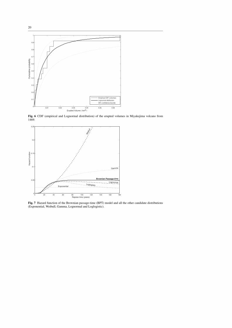
Using the eruption size data (volumes and VEI), it was not possible to find any evidence tosupport either a TPM or a SPM (highlighting that the unavoidable uncertainties in the vol-ume estimation or the possible recurrent behavior of the volcanic system may play an im-portant role to avoid the definition of a clear relationship between repose times and eruptedvolume). The question that arises is then, within this framework, how should the eruptedvolumes be distributed? We perform an analysis of the erupted volumes (within the periodof completeness of the catalog) and the results are summarized in Fig. 6. A Lognormal dis-tribution provides a good explanation of the erupted volume data (hypothesis not rejectedusing a one sample Kolmogorov-Smirnov test at a significance level of 0.05); it means thatthere exists a preferred or more common erupted volume (the mean erupted volume is 0.012±0.004 km3, assuming that not considerable bias exist in the volume database). In otherwords, we can consider that the logarithm of the erupted volumes are normally distributed.This result can support the hypothesis of a recurrent source model, as suggested by theBrownian passage-time distribution for the repose times, and may also explain the poor res-olution of the TPM, since if there is a preferred size and a preferred repose time, then thedata in a time-size space should tend to group in a cluster; from this point of view the BPTmodel would not be incompatible with a TPM model.

(FIGURE 6 (CDF OF ERUPTED VOLUMES...) SOMEWHERE AROUND HERE)

11

Table 2 Candidate distributions, PDF, estimated (MLE) model parameters and uncertainties, and AkaikeInformation Criteria (AIC)

Model Probability Parameters AICDensity (MLE)

Weibull θνθ tθ−1 e{−νθ tθ} ν−1 = 49.9 (±5.6) y. 107.3(ν , θ ) θ = 2.7 (±0.7)

Brownian(

µ2πα2t3

) 12 e

{− (t−µ)2

2α2 µt

}µ = 44.2 (±6.5) y. 108.3

Passage-time α = 0.51 (±0.01)(µ , α)

Gamma νθ tθ−1

Γ (θ) e−νt ν−1 = 9.1 (±3.8) 108.3(ν , θ ) θ = 4.9 (±1.9)

Lognormal 1σt

√2π e

{− (ln(t)−µ)2

2σ2

}µ = 3.68 (±0.15) 109.1

(µ , σ ) σ = 0.51 (±0.11)

Loglogistic eln(t)−µ

σ

σ(

1+eln(t)−µ

σ)2 µ = 3.72 (±0.15) 110.2

(µ , σ ) σ = 0.29 (±0.07)

Exponential ν e−νt ν−1 = 44.2 (±12.8) y. 116.9(ν)

Implications of Brownian model for Eruption Forecasting Assessment

As emerged from the model comparison analysis performed, five of the considered models(Weibull, BPT, Gamma, Lognormal, and Loglogistic) successfully described the Miyake-jima data set. Weibull, Gamma, Lognormal and Loglogistic models have been widely usedin volcanological literature, and their implications for the interpretation of the data havebeen discussed in many research papers (e.g., Bain 1978; Ho 1991, 1996; Bebbington andLai 1996a,b; Connor et al 2003; Watt et al 2007). Here we concentrate in analyze the intrin-sic characteristics of BPT model, and explore the implications that this tool may have foreruption forecasting.

Repose times for recurrent eruptive activity that may be described using a Brownian passage-time distribution may be used to define a model for time-dependent, long-term eruptionforecasting. This distribution has some noteworthy properties as (1) the probability of hav-ing renewed eruptive activity at time t = 0 is 0 (i.e. just after the last eruptive period); (2) ast → ∞ the hazard function is finite. In other words, it increases steadily from zero at t = 0to a finite maximum near the mean recurrence time. The first property should be analyzedcarefully since it may lead to misunderstanding if used improperly. As described in the in-troductory part, in our analysis we ignore eruption duration since we take the onset dateas the most physically meaningful; then we measure repose times from one onset date tothe next. Following this approach, our modeling intends to describe the waiting times ofthe long-term physical processes governing the onset of renewed volcanic activity. When an

12

eruption starts, the short-term behavior of eruptive activity might follow different patternsduring the gradual decline of activity; this means that sporadic eruptive episodes in a shorttime window after the onset of a new eruptive episode cannot be described using the formerlong-term model.

We now consider the random series of events t1 < t2 < .. . < ti . . ., and the repose timesτi = ti+1 − ti, (i = 1,2, . . .). If the sequence of random variables {τ} is independent anddistributed according to a function F(τ), then the original series of events {ti} is called arenewal process. For a history-dependent point process, the conditional intensity functionλ (t|Ht) of the form

λ (t|Ht) = h(x) =f (x)

1−F(x)=

f (x)S(x)

(4)

for x = (t − tL), defines the hazard function. Here, Ht is a history of occurrence times{ti; ti < t} before time t, including the information that no event occurred either in theintervals (t, ti+1) or in the interval (tL, t), and where tL is the last occurrence before theconsidered time t (e.g., Bain 1978; Ogata 1999). Then h(x) is the ratio of the probabilitydensity function f (x) to the survival function S(x) and it may be defined as the event rate attime t conditional on survival until time t (or later).

The hazard function describes instantaneous failure rate, or the conditional density of failureat time x given that no event occurred until time x. An increasing hazard function at time xindicates that an event is more likely to occur in a given increment of time (x,x+∆x) than itwould be in the same increment of time in an earlier age. It is also useful in the specificationof a point process since it may be directly linked with the probabilistic forecast of an eventoccurrence.

Fig. 7 shows the hazard function of the BPT model for Miyakejima volcano (see also Fig.5 for the corresponding cumulative distribution functions). Hazard functions of the othercandidate models are also included for comparison. For the BPT model, the failure rate iszero (0) immediately after an event, then it grows to a peak and then asymptotically tendsto a finite value at long times compared to the mean time. Fig. 7 can help to understandthe different behavior of the different candidate models and to compare them with the BPTmodel. The main characteristic of the Exponential model is the constant hazard function,implying a random occurrence of volcanic events in time. All the other models are moreor less similar up to the mean recurrence time, at which point their behavior diverges. Forexample, the hazard function of the Weibull model starts at zero and increases to infinity,while for the Lognormal model, the asymptotic failure rate goes to zero. The Gamma modelalso has a finite asymptotic failure rate, but the function grows more smoothly.

(FIGURE 7 (HAZARD FUNCTION OF BPT...) SOMEWHERE AROUND HERE)

We can calculate the conditional probability Pr(x, x+∆ t) that an eruption will happen in atime interval (x, x+∆ t], given an interval of x = (t − tL) years since the occurrence of theprevious eruption. Let T be the time to the next eruption, then

Pr(x, x+∆ t) = P(x < T ≤ (x+∆ t) | T > x) (5)

for x being the time since last eruption, as defined before. If F(τ) denotes the cumulativedistribution function of the repose times τ , then F(x) = Pr(T ≤ x), and F(x+∆ t) = Pr(T ≤

13

(x+∆ t)) for x ≥ 0, while the survival time function S(x) is S(x) = 1−F(x) = Pr(T> x), forx ≥ 0. Then, the probability that an eruption occurs in the next ∆ t interval is (e.g., Bowerset al 1997)

Pr(x, x+∆ t) =

∫ x+∆ tx f (s)ds1−F(x)

(6)

(note that for small ∆ t, Eq. 6 may be approximated to F(x+∆ t)−F(x)1−F(x) . Equation 6 can be in-

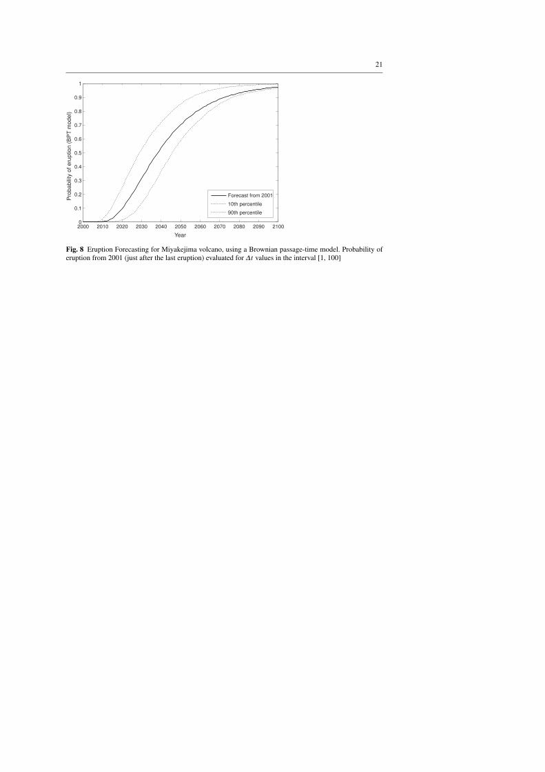
terpreted as the conditional probability that an eruption will occur in the time interval (x,x+∆ t), given an interval of x years since the occurrence of the last event. We can use thisequation to calculate probabilities of eruption and forecast future events. For example, Fig.8 is the evolution of Pr(x, x+∆ t) as seen from the time immediately after the last eruption in2000 for different values of ∆ t.

(FIGURE 8 (ERUPTION FORECASTING FOR MIYAKEJIMA...) SOMEWHERE AROUNDHERE)

Discussion

Renewal processes characterized by six different probabilistic models, plus a TPM and aSPM, have been applied to analyze the repose times between eruptive episodes of Miyake-jima volcano during the last 540 years (the period for which the catalog has been consid-ered complete). From our analysis we conclude that the two-parameters models (Weibull,Gamma, Lognormal, Loglogistic, and BPT) are able to explain the observed data, and showa better fit compared to the exponential distribution. While the former four models have beenwidely used in volcanological literature, the BPT model seems to be a new interesting alter-native to describe volcanological data. The BPT is based upon a simple physical model (theBrownian relaxation oscillator), and is parameterized by the mean rate of event occurrence,µ , and the aperiodicity about the mean, α . The Brownian passage-time family differs fromother usual candidate distributions for long-term eruption forecasting in that it may be morereadily interpreted in terms of the volcanic processes. The Brownian relaxation oscillatorand Brownian passage-time distribution connect together physical notions of unobservableloading and failure processes of a point process with observable response statistics (i.e. eventrecurrence in time).

The definition of a general model to describe eruptive activity is a difficult task due to dif-ferent factors such as the intrinsic complexity of eruptive processes and the difficulty ofgetting complete catalogs with sufficient observations. The BPT model may be consideredas a first-order approximation to describe different kinds of volcanic systems, which canspan from random volcanoes (Poisson-like processes), up to perfectly periodic systems. Thenon-homogeneous Poisson process model of Ho (1991), characterized by a Weibull distri-bution, was a first attempt of generalization to describe with a single model different kindsof processes. However, the Weibull is a model that possesses some intrinsically undesirablefeatures that are difficult to support from a physical point of view in volcanological applica-tions. For example, hazard rate functions of Weibull variates (Fig. 7) either start at zero andincrease to infinity or start at a finite value and decrease to zero. This asymptotic behaviormay be unrealistic in many physical systems and specifically in a volcanological application

14

may lead to unnecessary assumptions.

Conversely, the BPT model possesses many interesting features which make it a plausi-ble model to describe the activity of different volcanoes. If we consider its hazard function,the failure rate is zero immediately after an event. Then it grows to a peak and then de-clines to a finite asymptotic rate at times long compared to the mean rate. These are uniqueproperties among the set of candidate models considered. These properties provide a morerealistic asymptotic behavior of the failure rate. The BPT model may be regarded as a de-layed Poisson process (Ellsworth et al 1999), for which the failure rate is zero for a finitetime following an event and then steps up to an approximately constant failure rate at allsucceeding times.

To measure how much the BPT model approaches a Poisson-like or a periodic process,we can consider the α parameter. The more periodic the process, the more α approacheszero. The value α = 0.51 ± 0.01 found in this work for the aperiodicity in Miyakejimavolcano indicates a clear recurrent behavior in this volcanic system. To compare eruptiveactivity of different volcanoes with the results obtained in Miyakejima, we analyzed somecatalogs from published works in other volcanic areas: for instance, we considered the datafrom (1) Mt Ruapehu and (2) Mt. Ngauruhoe -New Zealand- (tables 2 and 3 in Bebbingtonand Lai (1996b)), (3) Kilauea and (4) Mauna Loa -Hawaii- (tables 1 and 2, respectively, inKlein (1982)), and (5) Mt. Etna (Marzocchi and Zaccarelli 2006).

Fig. 9 is a plot of the estimated parameters α and µ assuming a BPT model for the vol-canoes cited before. The µ (y axis) is just a scale parameter measuring the mean recurrencetime, whereas the (dimensionless) α parameter (x axis) may provide a good frameworkto compare different volcanic systems; for instance, if we consider the results in Fig. 9it is evident that all considered volcanoes but Miyakejima have α > 1. This is consistentwith the different results provided by the authors; for example, if we consider Mauna Loa(α = 1.28±0.4) and Kilauea (α = 3.02±1.49) volcanoes, α parameter indicates that thosevolcanoes have more Poisson-like or a clustered behavior, which is in agreement with theresults of Klein (1982) who concluded that Hawaiian eruptions are largely random phenom-ena displaying no periodicity. The high α value for Kilauea, could indicate clustering oferuptions (i.e. non-homogeneous Poisson processes). For Ruapehu (α = 1.26± 0.36) andNgauruhoe (α = 1.4± 0.33) volcanoes, the α parameter indicates also a Poisson-like be-havior, which is also in agreement with the results of Bebbington and Lai (1996b); in thosecases, the authors examined both the homogeneous Poisson and Weibull as possible modelsto describe the eruptive patterns of both volcanoes, concluding that both of them are morePoisson-like processes even if they are satisfactorily modeled by a Weibull renewal process.

(FIGURE 9 (ESTIMATED PARAMETERS (ALPHA AND MU)...) SOMEWHERE AROUNDHERE)

Another important consideration should be done with respect to the TPM/SPM models.As discussed in previous sections, it is not possible to define a clear relationship betweenrepose times and eruption sizes from Miyakejima volcano; additionally, we found that thereis a preferred erupted volume. Given the recurrent behavior of Miyakejima volcano (inferredfrom the α value of the BPT model), we argue that it is coherent that for preferred reposetimes it is possible to have preferred erupted volumes. It means that BPT model may be usedin volcanoes that tend to produce eruptions of similar sizes. It implies also that it is possible

15

that a TPM or SPM model could coexist within our BPT model for recurrent volcanic activ-ity. In fact, The BRO may be extended to models that are not renewal processes; in particularstochastic versions of TPM and SPM may be derived from randomized boundary conditionsin the Brownian oscillator (Matthews et al 2002).

Concluding remarks

The intrinsic complexity of volcanic systems motivates the definition of probability modelsas mathematical structures to describe the response of the considered systems. Here, we putforward a new model borrowed by seismology named Brownian Passage Time (BPT). Theapplication to the past eruptive activity of Miyakejima volcano shows that BPT fits signif-icantly better the eruptive time occurrence than the exponential distribution. Despite the fitis comparable to the one obtained by the other two-parameters models considered, BPT hassome interesting features that allow us to interpret straightforwardly and more realisticallythe long-term behavior of the volcano.

The Brownian passage-time family of distributions describes the response of a conceptualphysical system defined as a Brownian relaxation oscillator (BRO). BRO and BPT togetherconnect physical notions of unobservable loading and failure processes of a point processwith observable event-time statistics. BPT model is characterized by two parameters: themean repose time (µ) and the aperiodicity of the mean (α). While µ is just an scale param-eter that provides information about the typical frequency at which eruptive events occur,α is a dimensionless parameter that measures the aperiodicity of the mean response of thesystem, and for this reason this parameter may be useful to compare different volcanoesspanning from periodic-like to Poisson-like systems.

For the Miyakejima volcano, the mean repose time is µ = 44.2 ± 6.5 years, while thedimensionless aperiodicity parameter is α = 0.51 ±0.01. This value for α parameter is anevidence of recurrent eruptive activity of Miyakejima volcano, and the first such recognizedexample.

The BPT model provides some insights for time-dependent, long-term eruption forecast-ing. For instance, if we consider the hazard function, some noteworthy properties can bedefined: the probability of having renewed eruptive activity just after an eruptive cycle isvery low, then it increases steadily from zero to a finite maximum near the mean recurrencetime. Finally, for times greater than the mean recurrence time the hazard function tends toa finite constant value, indicating that for long repose times the system tends to behave as aPoisson process.

Acknowledgements The manuscript was greatly improved by helpful reviews and constructive commentsfrom G. Wadge, J. Phillips and an anonymous reviewer. Critical and useful comments of an earlier version ofthe manuscript were made by L. Sandri and J. Selva. A. Garcia thanks the staff of NIED’s Volcano ResearchDepartment for their friendly hospitality during his stay in Japan; A. Garcia’s stay in Japan was funded bythe Marco Polo program of the Universita di Bologna (Italy).

16

References

Akaike H (1974) A new look at the statistical model identification. IEEE Trans Automat Contr AC 19:716–723

Bain LJ (1978) Statistical analysis of reliability and life-testing models, Theory and Methods. Marcel Dekker,New York

Bebbington MS, Lai CD (1996a) On nonhomogeneous models for volcanic eruptions. Math Geol 28:585–600Bebbington MS, Lai CD (1996b) Statistical analysis of new zealand volcanic occurrence data. J Vol-

canol Geotherm Res 74:101–110Bowers N, Gerber H, Hickman J, Jones D, Nesbitt C (1997) Actuarial Mathematics, 2nd edn. Society of

ActuariesBurt ML, Wadge G, Scott WA (1994) Simple stochastic modelling of the eruption history of a basaltic vol-

cano: Nyamuragira, Zaire. Bull Volcanol 56:87–97Coles S, Sparks R (2006) Extreme value methods for modeling historical series of large volcanic magni-

tudes. In: Mader H, Coles S, Connor C, Connor L (eds) Statistics in Volcanology, IAVCEI Publications,Geological Society, London, pp 47–56

Connor CB, Sparks RSJ, Mason RM, Bonadonna C (2003) Exploring links between physical and probabilisticmodels of volcanic eruptions: The soufriere hills volcano, montserrat. Geophys Res Lett 30(13), DOI10.1029/2003GL017384

Cox DR, Lewis PAW (1966) The statistical analysis of Series of Events. Mathuen, New YorkDe la Cruz-Reyna S (1991) Poisson-distributed patterns of explosive eruptive activity. Bull Volcanol 54:57–67Ellsworth WL, Matthews MV, Nadeau RM, Nishenko SP, Reasenberg PA, Simpson RW (1999) A

physically based earthquake recurrence model for estimation of long-term earthquake probabilities.U S Geol Surv Open-File Rept pp 99–522

Ho C (1991) Nonhomogeneous Poisson model for volcanic eruptions. Math Geol 23(2):167–173Ho CH (1996) Volcanic time-trend analysis. J Volcanol Geotherm Res 74(3-4):171–177Klein F (1982) Patterns of historical eruptions at Hawaiian volcanoes. J Volcanol Geotherm Res 12(1-2):1–35,

DOI 10.1016/0377-0273(82)90002-6Marzocchi W, Zaccarelli L (2006) A quantitative model for time-size distribution of eruptions. J Geophys Res

111(B04204), DOI 10.1029/2005JB003709Matthews M, Ellsworth W, Reasenberg P (2002) A Brownian model for recurrent earthquakes.

Bull Seism Soc Am 92(6):2233–2250, DOI 10.1785/0120010267Mulargia F, Tinti S (1985) Seismic sample areas defined from incomplete catalogs: An application to the

italian territory. Phys Earth Planet Inter 40(4):273–300Mulargia F, Tinti S, Boschi E (1985) A statistical analysis of flank eruptions on Etna volcano. J Vol-

canol Geotherm Res 23(3-4):263–272Mulargia F, Gasperini P, Tinti E (1987) Identifying different regimes in eruptive activity: an application to

Etna volcano. J Volcanol Geotherm Res 34(1-2):89–106Nakada S, Nagai M, Kaneko T, Nozawa A, Suzuki-Kamata K (2005) Chronology and prod-

ucts of the 2000 eruption of Miyakejima volcano, Japan. Bull Volcanol 67(3):205–218, URLhttp://www.springerlink.com/content/cj0d4tkcfamr7f32

Newhall C, Self S (1982) The Volcanic Explosivity Index (VEI): An estimate of explosive magnitude forhistorical volcanism. J Geophys Res 87(C2):1231–1238

Ogata Y (1999) Estimating the hazard of ruptire using uncertain occurrence times of paleoearthquakes. J Geo-phys Res 104(B8):17,995–18,014

Sandri L, Marzocchi W, Gasperini P (2005) Some insights on the occurrence of recent volcanic eruptions ofMount Etna volcano (Sicily, Italy). Geophys J Int 163(3):1203–1218

Simkin T, Siebert L (2002 onwards) Volcanoes of the World: an Illustrated Catalog of Holocene Volca-noes and their Eruptions. Smithsonian Institution, Global Volcanism Program Digital Information Series,GVP-3, (http://www.volcano.si.edu/world/)

Tsukui M, Suzuki Y (1998) Eruptive history of Miyakejima volcano during the last 7000 years. Bull Vol-canol Soc Japan 43:149–166

Ueda H, Fujita E, Ukawa M, Yamamoto E, Irwan M, Kimata F (2005) Magma intrusion and discharge processat the initial stage of the 2000 activity of Miyakejima, Central Japan, inferred from tilt and GPS data.Geophys J Int 161(3):891–906, DOI 10.1111/j.1365-246X.2005.02602.x

Watt SFL, Mather TA, Pyle DM (2007) Vulcanian explosion cycles: Patterns and predictability. Geology35(9):839–842, DOI 10.1130/G23562A.1

Wickman FE (1976) Markov models of repose-period patterns of volcanoes, in: Random Process in Geology,Springer, New York, pp 135–161

17

135° E 140°E 145°E

30° N

35° N

40° N

34.12°

34.10°

34.08°

34.06°

34.04°

139.48° 139.50° 139.52° 139.54° 139.56°

Japan

Tokyo

Miyakejima

IzuIslands

Fig. 1 Map of the Miyakejima volcano and location in the Izu island group, Japan.

18

-6000 -5000 -4000 -3000 -2000 -1000 0 1000 2000 30000

0.2

0.4

0.6

0.8

1

1.2

Eruption Date (Year)

Cu

mu

lative

eru

pte

d V

olu

me

(km

3)

0

5

10

15

20

25

30

Cu

mu

lative

Nu

mb

er

of

Eru

ptio

ns

CHPT 1(s.l. 0.01)

(a)

(b)

Fig. 2 (a) Cumulative number of eruptions with time, and Change Point analysis, Miyakejima volcano. (b)The cumulative volume of erupted material (DRE) is also shown for reference.

1.3 1.4 1.5 1.6 1.7 1.8-4.0

-3.5

-3.0

-2.5

-2.0

-1.5

-1.0

-0.5

0

Slope = -0.176 (± 0.80)

R2 = 0.005

F = 0.049 (F-test)

(a)

Log (

Eru

pte

d V

olu

me (

Km

3)

)

Log(Time since previous eruption)

Size Predictable Model (SPM)

Slope = -0.500 (± 0.79)

R2 = 0.038

F = 0.397 (F-test)

(b)

Log(Time to following eruption)

Time Predictable Model (TPM)

-4.0

-3.5

-3.0

-2.5

-2.0

-1.5

-1.0

-0.5

0

Log (

Eru

pte

d V

olu

me (

Km

3)

)

1.3 1.4 1.5 1.6 1.7 1.8

Fig. 3 Plot of times since previous eruption (a) and times to the following one (b) against the erupted volume(in km3) of Miyakejima volcano, to test a Size Predictable Model (a) and a Time Predictable Model (b),respectively.

19

20 25 30 35 40 45 50 55 60 650

0.1

0.2

0.3

0.4

0.5

0.6

0.7

0.8

0.9

1

Repose time (Years)

Cum

ula

tive p

robabili

ty

Repose times (empirical CDF)

95% confidence bounds

CDF - Exponential distrib

ution

Fig. 4 Cumulative distribution function (CDF) of the best fitting Exponential distribution, and the empiricalCDF of the observed repose times.

20 25 30 35 40 45 50 55 60 650

0.1

0.2

0.3

0.4

0.5

0.6

0.7

0.8

0.9

1

Repose time (years)

Cum

ula

tive p

robabili

ty

Repose times

(empirical CDF)

Exponential

LogNormal

GammaWeibull

95% confidence bounds (W

eibull)

BPT

Loglogistic

Fig. 5 Plot of the Cumulative Distribution Function (CDF) of Brownian passage-time, Weibull, Lognormal,Gamma and Loglogistic models, and the empirical CDF of the observed repose times. The CDF of the Expo-nential model is also included for reference.

20

0.01 0.02 0.03 0.04 0.05 0.060

0.1

0.2

0.3

0.4

0.5

0.6

0.7

0.8

0.9

1

Erupted Volume ( km3 )

Cu

mu

lative

pro

ba

bili

ty

Empirical CDF (volumes)

Lognormal distribution

95% confidence bounds

Fig. 6 CDF (empirical and Lognormal distribution) of the erupted volumes in Miyakejima volcano from1469.

0 20 40 60 80 100 120 140 160 1800

0.05

0.1

0.15

0.2

0.25

Repose time (years)

Hazard

function

Brownian Passage-time

Loglogistic

Gamma

Lognormal

Weib

ull

Exponential

Fig. 7 Hazard function of the Brownian passage-time (BPT) model and all the other candidate distributions(Exponential, Weibull, Gamma, Lognormal and Loglogistic).

21

2000 2010 2020 2030 2040 2050 2060 2070 2080 2090 21000

0.1

0.2

0.3

0.4

0.5

0.6

0.7

0.8

0.9

1

Year

Pro

ba

bili

ty o

f e

rup

tio

n (

BP

T m

od

el)

Forecast from 2001

10th percentile

90th percentile

Fig. 8 Eruption Forecasting for Miyakejima volcano, using a Brownian passage-time model. Probability oferuption from 2001 (just after the last eruption) evaluated for ∆ t values in the interval [1, 100]

22

0 0.5 1 1.5 2 2.5 3 3.5 4 4.5

101

102

Ruapehu

Ngauruhoe

Kilauea

Mauna Loa

Miyakejima

Etna

Me

an

re

cu

rre

nce

tim

e µ

(ye

ars

)

α (dimensionless)

5

50

"Periodic-like"

behavior

"Poisson-like" behavior

(homogeneous/nonhomogeneous)

Fig. 9 Estimated parameters (α and µ) of the Brownian passage-time model for different volcanoes: Miyake-jima (Japan), Etna (Italy), Ruapehu and Ngauruhoe (New Zealand), Mauna Loa and Kulauea (Hawaii). Forthe source of the data see the text.