Page 1
Approximation of the Bessel functionA case study
D.S. Karachalios, I.V. Gosea, A.C. Antoulas
February 28, 2018
Affiliations:MPI Magdeburg, Rice University Houston
12th Elgersburg Workshop
Partners:
Page 2
Outline
Introduction and motivation.
Overview of the approximation methods we apply:
1 The Loewner Framework.
2 The AAA algorithm.
3 The Vector Fitting (VF) method.
Numerical results and comparison among the methods.
Further examples (Physical & Artificial).
Conclusion and further developments.
Dimitris, [email protected] Irrational Approximation 2/26
Page 3
Introduction
1. In general, model order reduction (MOR) is used to transform large,complex models (n) of time dependent processes into smaller(k n), simpler models that are still capable or representingaccurately the behavior of the original process under a variety ofconditions.
2. In particular, interpolatory model reduction methods constructreduced models whose (rational) transfer function matches that of theoriginal system at selected interpolation points.
3. Irrational transfer function correspond to infinite-dimensionaldynamical system. Is it possible to approximate such a function(without performing any spatial discretization)?
Main tool: The Loewner framework → data driven MOR method.Computes an independent linear realization (E,A,B,C).
Dimitris, [email protected] Irrational Approximation 3/26
Page 4
Introduction
1. In general, model order reduction (MOR) is used to transform large,complex models (n) of time dependent processes into smaller(k n), simpler models that are still capable or representingaccurately the behavior of the original process under a variety ofconditions.
2. In particular, interpolatory model reduction methods constructreduced models whose (rational) transfer function matches that of theoriginal system at selected interpolation points.
3. Irrational transfer function correspond to infinite-dimensionaldynamical system. Is it possible to approximate such a function(without performing any spatial discretization)?
Main tool: The Loewner framework → data driven MOR method.Computes an independent linear realization (E,A,B,C).
Dimitris, [email protected] Irrational Approximation 3/26
Page 5
Introduction
1. In general, model order reduction (MOR) is used to transform large,complex models (n) of time dependent processes into smaller(k n), simpler models that are still capable or representingaccurately the behavior of the original process under a variety ofconditions.
2. In particular, interpolatory model reduction methods constructreduced models whose (rational) transfer function matches that of theoriginal system at selected interpolation points.
3. Irrational transfer function correspond to infinite-dimensionaldynamical system. Is it possible to approximate such a function(without performing any spatial discretization)?
Main tool: The Loewner framework → data driven MOR method.Computes an independent linear realization (E,A,B,C).
Dimitris, [email protected] Irrational Approximation 3/26
Page 6
Introduction
1. In general, model order reduction (MOR) is used to transform large,complex models (n) of time dependent processes into smaller(k n), simpler models that are still capable or representingaccurately the behavior of the original process under a variety ofconditions.
2. In particular, interpolatory model reduction methods constructreduced models whose (rational) transfer function matches that of theoriginal system at selected interpolation points.
3. Irrational transfer function correspond to infinite-dimensionaldynamical system. Is it possible to approximate such a function(without performing any spatial discretization)?
Main tool: The Loewner framework → data driven MOR method.
Computes an independent linear realization (E,A,B,C).
Dimitris, [email protected] Irrational Approximation 3/26
Page 7
Introduction
1. In general, model order reduction (MOR) is used to transform large,complex models (n) of time dependent processes into smaller(k n), simpler models that are still capable or representingaccurately the behavior of the original process under a variety ofconditions.
2. In particular, interpolatory model reduction methods constructreduced models whose (rational) transfer function matches that of theoriginal system at selected interpolation points.
3. Irrational transfer function correspond to infinite-dimensionaldynamical system. Is it possible to approximate such a function(without performing any spatial discretization)?
Main tool: The Loewner framework → data driven MOR method.Computes an independent linear realization (E,A,B,C).
Dimitris, [email protected] Irrational Approximation 3/26
Page 8
Motivation
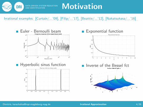
Irrational examples: [Curtain/...’09], [Filip/...’17], [Beattie/...’12], [Nakatsukasa/...’16]. . . . . . . . . . . . . . . . . . . . . . . . . . . . . . . . . . . . . . . . . . . . . . . . . . . . . . . . . . . . . . . . . . . . . . . . . . . . . . . . . . . . . . . . . . .
Euler - Bernoulli beam
frequency (Hz)101 102 103 104 105
Mag
nitu
de
10-6
10-4
10-2
100
102Frequency response of the original beam model
Hyperbolic sinus function
x-1 -0.8 -0.6 -0.4 -0.2 0 0.2 0.4 0.6 0.8 1
H(x
)
0
0.2
0.4
0.6
0.8
1Function with two sharp peaks
Exponential function
x0 1 2 3 4 5 6 7 8 9 10
H(x
)
0
0.2
0.4
0.6
0.8
1Exponential function
Inverse of the Bessel fct
Dimitris, [email protected] Irrational Approximation 4/26
Page 9
Motivation
Irrational examples: [Curtain/...’09], [Filip/...’17], [Beattie/...’12], [Nakatsukasa/...’16]. . . . . . . . . . . . . . . . . . . . . . . . . . . . . . . . . . . . . . . . . . . . . . . . . . . . . . . . . . . . . . . . . . . . . . . . . . . . . . . . . . . . . . . . . . .
Euler - Bernoulli beam
frequency (Hz)101 102 103 104 105
Mag
nitu
de
10-6
10-4
10-2
100
102Frequency response of the original beam model
Hyperbolic sinus function
x-1 -0.8 -0.6 -0.4 -0.2 0 0.2 0.4 0.6 0.8 1
H(x
)
0
0.2
0.4
0.6
0.8
1Function with two sharp peaks
Exponential function
x0 1 2 3 4 5 6 7 8 9 10
H(x
)
0
0.2
0.4
0.6
0.8
1Exponential function
Inverse of the Bessel fct
Dimitris, [email protected] Irrational Approximation 4/26
Page 10
Motivation
Irrational examples: [Curtain/...’09], [Filip/...’17], [Beattie/...’12], [Nakatsukasa/...’16]. . . . . . . . . . . . . . . . . . . . . . . . . . . . . . . . . . . . . . . . . . . . . . . . . . . . . . . . . . . . . . . . . . . . . . . . . . . . . . . . . . . . . . . . . . .
Euler - Bernoulli beam
frequency (Hz)101 102 103 104 105
Mag
nitu
de
10-6
10-4
10-2
100
102Frequency response of the original beam model
Hyperbolic sinus function
x-1 -0.8 -0.6 -0.4 -0.2 0 0.2 0.4 0.6 0.8 1
H(x
)
0
0.2
0.4
0.6
0.8
1Function with two sharp peaks
Exponential function
x0 1 2 3 4 5 6 7 8 9 10
H(x
)
0
0.2
0.4
0.6
0.8
1Exponential function
Inverse of the Bessel fct
Dimitris, [email protected] Irrational Approximation 4/26
Page 11
Motivation
Irrational examples: [Curtain/...’09], [Filip/...’17], [Beattie/...’12], [Nakatsukasa/...’16]. . . . . . . . . . . . . . . . . . . . . . . . . . . . . . . . . . . . . . . . . . . . . . . . . . . . . . . . . . . . . . . . . . . . . . . . . . . . . . . . . . . . . . . . . . .
Euler - Bernoulli beam
frequency (Hz)101 102 103 104 105
Mag
nitu
de
10-6
10-4
10-2
100
102Frequency response of the original beam model
Hyperbolic sinus function
x-1 -0.8 -0.6 -0.4 -0.2 0 0.2 0.4 0.6 0.8 1
H(x
)
0
0.2
0.4
0.6
0.8
1Function with two sharp peaks
Exponential function
x0 1 2 3 4 5 6 7 8 9 10
H(x
)
0
0.2
0.4
0.6
0.8
1Exponential function
Inverse of the Bessel fct
Dimitris, [email protected] Irrational Approximation 4/26
Page 12
Motivation
Irrational examples: [Curtain/...’09], [Filip/...’17], [Beattie/...’12], [Nakatsukasa/...’16]. . . . . . . . . . . . . . . . . . . . . . . . . . . . . . . . . . . . . . . . . . . . . . . . . . . . . . . . . . . . . . . . . . . . . . . . . . . . . . . . . . . . . . . . . . .
Euler - Bernoulli beam
frequency (Hz)101 102 103 104 105
Mag
nitu
de
10-6
10-4
10-2
100
102Frequency response of the original beam model
Hyperbolic sinus function
x-1 -0.8 -0.6 -0.4 -0.2 0 0.2 0.4 0.6 0.8 1
H(x
)
0
0.2
0.4
0.6
0.8
1Function with two sharp peaks
Exponential function
x0 1 2 3 4 5 6 7 8 9 10
H(x
)
0
0.2
0.4
0.6
0.8
1Exponential function
Inverse of the Bessel fct
Dimitris, [email protected] Irrational Approximation 4/26
Page 13
Motivation and Methods
What if we don’t have access to the matrix realization or to theexplicit form of the transfer function? (Only data provided)
Answer
→ Data Driven approach!
Take measurements and use:
1 The Loewner framework - [Mayo/Antoulas ’07]
2 The AAA algorithm - [Nakatsukasa/Sete/Trefethen ’16]
3 The Vector Fitting method - [Gustavsen/Semlyen ’99]
Dimitris, [email protected] Irrational Approximation 5/26
Page 14
Motivation and Methods
What if we don’t have access to the matrix realization or to theexplicit form of the transfer function? (Only data provided)
Answer → Data Driven approach!
Take measurements and use:
1 The Loewner framework - [Mayo/Antoulas ’07]
2 The AAA algorithm - [Nakatsukasa/Sete/Trefethen ’16]
3 The Vector Fitting method - [Gustavsen/Semlyen ’99]
Dimitris, [email protected] Irrational Approximation 5/26
Page 15
Motivation and Methods
What if we don’t have access to the matrix realization or to theexplicit form of the transfer function? (Only data provided)
Answer → Data Driven approach!
Take measurements and use:
1 The Loewner framework - [Mayo/Antoulas ’07]
2 The AAA algorithm - [Nakatsukasa/Sete/Trefethen ’16]
3 The Vector Fitting method - [Gustavsen/Semlyen ’99]
Dimitris, [email protected] Irrational Approximation 5/26
Page 16
Motivation and Methods
What if we don’t have access to the matrix realization or to theexplicit form of the transfer function? (Only data provided)
Answer → Data Driven approach!
Take measurements and use:
1 The Loewner framework - [Mayo/Antoulas ’07]
2 The AAA algorithm - [Nakatsukasa/Sete/Trefethen ’16]
3 The Vector Fitting method - [Gustavsen/Semlyen ’99]
Dimitris, [email protected] Irrational Approximation 5/26
Page 17
Motivation and Methods
What if we don’t have access to the matrix realization or to theexplicit form of the transfer function? (Only data provided)
Answer → Data Driven approach!
Take measurements and use:
1 The Loewner framework - [Mayo/Antoulas ’07]
2 The AAA algorithm - [Nakatsukasa/Sete/Trefethen ’16]
3 The Vector Fitting method - [Gustavsen/Semlyen ’99]
Dimitris, [email protected] Irrational Approximation 5/26
Page 18
Motivation and Methods
What if we don’t have access to the matrix realization or to theexplicit form of the transfer function? (Only data provided)
Answer → Data Driven approach!
Take measurements and use:
1 The Loewner framework - [Mayo/Antoulas ’07]
2 The AAA algorithm - [Nakatsukasa/Sete/Trefethen ’16]
3 The Vector Fitting method - [Gustavsen/Semlyen ’99]
Dimitris, [email protected] Irrational Approximation 5/26
Page 19
Overview of the methods
A simple SISO example - (spring - mass - damper). . . . . . . . . . . . . . . . . . . . . . . . . . . . . . . . . . . . . . . . . . . . . . . . . . . . . . . . . . . . . . . . . . . . . . . . . . . . . . . . . . . . . . . . . . .
Spring-mass-damper equation
mx(t) + dx(t) + kx(t) = F (t)
State variable: x1 = x,x2 = x, output y = x.x1 = x2mx2 = −kx1 − dx2 + Fu = F , y = x1
Compact form - System
x(t) = Ax(t) + Bu(t),y(t) = Cx(t)
Where x =
[xx
],
A =
[0 1
− km − d
m
],B =
[01m
], C =[1 0]
Transfer Function
H(s) = C(sI−A)−1B =1
ms2 + ds+ k
We assume that: m=1, d=1 and k=1.
Dimitris, [email protected] Irrational Approximation 6/26
Page 20
Overview of the methods
A simple SISO example - (spring - mass - damper). . . . . . . . . . . . . . . . . . . . . . . . . . . . . . . . . . . . . . . . . . . . . . . . . . . . . . . . . . . . . . . . . . . . . . . . . . . . . . . . . . . . . . . . . . .
Spring-mass-damper equation
mx(t) + dx(t) + kx(t) = F (t)
State variable: x1 = x,x2 = x, output y = x.x1 = x2mx2 = −kx1 − dx2 + Fu = F , y = x1
Compact form - System
x(t) = Ax(t) + Bu(t),y(t) = Cx(t)
Where x =
[xx
],
A =
[0 1
− km − d
m
],B =
[01m
], C =[1 0]
Transfer Function
H(s) = C(sI−A)−1B =1
ms2 + ds+ k
We assume that: m=1, d=1 and k=1.
Dimitris, [email protected] Irrational Approximation 6/26
Page 21
Overview of the methods
A simple SISO example - (spring - mass - damper). . . . . . . . . . . . . . . . . . . . . . . . . . . . . . . . . . . . . . . . . . . . . . . . . . . . . . . . . . . . . . . . . . . . . . . . . . . . . . . . . . . . . . . . . . .
Spring-mass-damper equation
mx(t) + dx(t) + kx(t) = F (t)
State variable: x1 = x,x2 = x, output y = x.x1 = x2mx2 = −kx1 − dx2 + Fu = F , y = x1
Compact form - System
x(t) = Ax(t) + Bu(t),y(t) = Cx(t)
Where x =
[xx
],
A =
[0 1
− km − d
m
],B =
[01m
], C =[1 0]
Transfer Function
H(s) = C(sI−A)−1B =1
ms2 + ds+ k
We assume that: m=1, d=1 and k=1.
Dimitris, [email protected] Irrational Approximation 6/26
Page 22
Overview of the methods
A simple SISO example - (spring - mass - damper). . . . . . . . . . . . . . . . . . . . . . . . . . . . . . . . . . . . . . . . . . . . . . . . . . . . . . . . . . . . . . . . . . . . . . . . . . . . . . . . . . . . . . . . . . .
Spring-mass-damper equation
mx(t) + dx(t) + kx(t) = F (t)
State variable: x1 = x,x2 = x, output y = x.x1 = x2mx2 = −kx1 − dx2 + Fu = F , y = x1
Compact form - System
x(t) = Ax(t) + Bu(t),y(t) = Cx(t)
Where x =
[xx
],
A =
[0 1
− km − d
m
],B =
[01m
], C =[1 0]
Transfer Function
H(s) = C(sI−A)−1B =1
ms2 + ds+ k
We assume that: m=1, d=1 and k=1.
Dimitris, [email protected] Irrational Approximation 6/26
Page 23
Overview of the methods
Method 1: The Loewner Framework - [Mayo/Antoulas ’07]. . . . . . . . . . . . . . . . . . . . . . . . . . . . . . . . . . . . . . . . . . . . . . . . . . . . . . . . . . . . . . . . . . . . . . . . . . . . . . . . . . . . . . . . . . .
Theory
Given: a row array of pairs ofcomplex numbers:
(ωk, Sk) : k = 1, ..., N
with ωk ∈ C, Sk ∈ C. We canpartition the data in two sets:
left data: (µj , νj), j = 1, ..., p
right data: (λi, wi), i = 1, ...,m
The objective is to find H(s) ∈ Csuch that:
H(λi) = wi and H (µj) = νj
Example
Sample the transfer function of thespring-mass-damper:ω =
[1 2 3 4 5 6 7 8
]S =
[13
17
113
121
131
143
157
173
]• left data:
µ =[
1 3 5 7]
V =[
13
113
131
157
]• right data:
λ =[
2 4 6 8]
W =[
17
121
143
173
]
Dimitris, [email protected] Irrational Approximation 7/26
Page 24
Overview of the methods
Method 1: The Loewner Framework - [Mayo/Antoulas ’07]. . . . . . . . . . . . . . . . . . . . . . . . . . . . . . . . . . . . . . . . . . . . . . . . . . . . . . . . . . . . . . . . . . . . . . . . . . . . . . . . . . . . . . . . . . .
Theory
Given: a row array of pairs ofcomplex numbers:
(ωk, Sk) : k = 1, ..., N
with ωk ∈ C, Sk ∈ C. We canpartition the data in two sets:
left data: (µj , νj), j = 1, ..., p
right data: (λi, wi), i = 1, ...,m
The objective is to find H(s) ∈ Csuch that:
H(λi) = wi and H (µj) = νj
Example
Sample the transfer function of thespring-mass-damper:ω =
[1 2 3 4 5 6 7 8
]S =
[13
17
113
121
131
143
157
173
]• left data:
µ =[
1 3 5 7]
V =[
13
113
131
157
]• right data:
λ =[
2 4 6 8]
W =[
17
121
143
173
]Dimitris, [email protected] Irrational Approximation 7/26
Page 25
Overview of the methods
Method 1: The Loewner Framework - [Mayo/Antoulas ’07]. . . . . . . . . . . . . . . . . . . . . . . . . . . . . . . . . . . . . . . . . . . . . . . . . . . . . . . . . . . . . . . . . . . . . . . . . . . . . . . . . . . . . . . . . . .
Theory
The Loewner matrix L ∈ Cp×m, isdefined as:
L =
v1−w1
µ1−λ1· · · v1−wm
µ1−λm
.... . .
...vp−w1
µp−λ1· · · vp−wm
µp−λm
The shifted Loewner matrixLs ∈ Cp×m, is defined as:
Ls =
µ1v1−w1λ1
µ1−λ1· · · µ1v1−wmλm
µ1−λm
.... . .
...µpvp−w1λ1
µp−λ1· · · µpvp−wmλm
µp−λm
Example
The Loewner matrix
L =
− 4
21 − 221 − 8
129 − 10219
− 691 − 8
273 − 10559 − 12
949
− 8217 − 10
651 − 121333 − 14
2263
− 10399 − 4
399 − 142451 − 16
4161
The shifted Loewner matrix
Ls =
− 1
21 − 121 − 5
129 − 7219
− 591 − 11
273 − 17559 − 23
949
− 9217 − 19
651 − 291333 − 39
2263
− 13399 − 3
133 − 412451 − 55
4161
Dimitris, [email protected] Irrational Approximation 8/26
Page 26
Overview of the methods
Method 1: The Loewner Framework - [Mayo/Antoulas ’07]. . . . . . . . . . . . . . . . . . . . . . . . . . . . . . . . . . . . . . . . . . . . . . . . . . . . . . . . . . . . . . . . . . . . . . . . . . . . . . . . . . . . . . . . . . .
Theory
The Loewner matrix L ∈ Cp×m, isdefined as:
L =
v1−w1
µ1−λ1· · · v1−wm
µ1−λm
.... . .
...vp−w1
µp−λ1· · · vp−wm
µp−λm
The shifted Loewner matrixLs ∈ Cp×m, is defined as:
Ls =
µ1v1−w1λ1
µ1−λ1· · · µ1v1−wmλm
µ1−λm
.... . .
...µpvp−w1λ1
µp−λ1· · · µpvp−wmλm
µp−λm
Example
The Loewner matrix
L =
− 4
21 − 221 − 8
129 − 10219
− 691 − 8
273 − 10559 − 12
949
− 8217 − 10
651 − 121333 − 14
2263
− 10399 − 4
399 − 142451 − 16
4161
The shifted Loewner matrix
Ls =
− 1
21 − 121 − 5
129 − 7219
− 591 − 11
273 − 17559 − 23
949
− 9217 − 19
651 − 291333 − 39
2263
− 13399 − 3
133 − 412451 − 55
4161
Dimitris, [email protected] Irrational Approximation 8/26
Page 27
Overview of the methods
Method 1: The Loewner Framework - [Mayo/Antoulas ’07]. . . . . . . . . . . . . . . . . . . . . . . . . . . . . . . . . . . . . . . . . . . . . . . . . . . . . . . . . . . . . . . . . . . . . . . . . . . . . . . . . . . . . . . . . . .
The following results allow us to construct reduced order models.
Theorem
If (L,Ls) is regular, then E = −L, A = −Ls, B = V, C = W is arealization of the data. Hence, H(z) = W(Ls − zL)−1V is the requiredinterpolant.
In the case of redundant data we perform a rank revealing SVD of:[L,Ls
]or
[LLs
]then
[L,Ls
]= YΣ`X
∗ and
[LLs
]= YΣrX
∗.
Theorem
The quadruple E = −Y∗LX, A = −Y∗LsX, B = Y∗V, C = WX, isthe realization of an approximate data interpolant.
Remark: Above is the SISO case. Moreover, the Loewner Framework can beapplied also for MIMO case via tangential interpolation.
Dimitris, [email protected] Irrational Approximation 9/26
Page 28
Overview of the methods
Method 1: The Loewner Framework - [Mayo/Antoulas ’07]. . . . . . . . . . . . . . . . . . . . . . . . . . . . . . . . . . . . . . . . . . . . . . . . . . . . . . . . . . . . . . . . . . . . . . . . . . . . . . . . . . . . . . . . . . .
The following results allow us to construct reduced order models.
Theorem
If (L,Ls) is regular, then E = −L, A = −Ls, B = V, C = W is arealization of the data. Hence, H(z) = W(Ls − zL)−1V is the requiredinterpolant.
In the case of redundant data we perform a rank revealing SVD of:[L,Ls
]or
[LLs
]then
[L,Ls
]= YΣ`X
∗ and
[LLs
]= YΣrX
∗.
Theorem
The quadruple E = −Y∗LX, A = −Y∗LsX, B = Y∗V, C = WX, isthe realization of an approximate data interpolant.
Remark: Above is the SISO case. Moreover, the Loewner Framework can beapplied also for MIMO case via tangential interpolation.
Dimitris, [email protected] Irrational Approximation 9/26
Page 29
Overview of the methods
Method 1: The Loewner Framework - [Mayo/Antoulas ’07]. . . . . . . . . . . . . . . . . . . . . . . . . . . . . . . . . . . . . . . . . . . . . . . . . . . . . . . . . . . . . . . . . . . . . . . . . . . . . . . . . . . . . . . . . . .
The following results allow us to construct reduced order models.
Theorem
If (L,Ls) is regular, then E = −L, A = −Ls, B = V, C = W is arealization of the data. Hence, H(z) = W(Ls − zL)−1V is the requiredinterpolant.
In the case of redundant data we perform a rank revealing SVD of:[L,Ls
]or
[LLs
]then
[L,Ls
]= YΣ`X
∗ and
[LLs
]= YΣrX
∗.
Theorem
The quadruple E = −Y∗LX, A = −Y∗LsX, B = Y∗V, C = WX, isthe realization of an approximate data interpolant.
Remark: Above is the SISO case. Moreover, the Loewner Framework can beapplied also for MIMO case via tangential interpolation.
Dimitris, [email protected] Irrational Approximation 9/26
Page 30
Overview of the methods
Method 1: The Loewner Framework - [Mayo/Antoulas ’07]. . . . . . . . . . . . . . . . . . . . . . . . . . . . . . . . . . . . . . . . . . . . . . . . . . . . . . . . . . . . . . . . . . . . . . . . . . . . . . . . . . . . . . . . . . .
The following results allow us to construct reduced order models.
Theorem
If (L,Ls) is regular, then E = −L, A = −Ls, B = V, C = W is arealization of the data. Hence, H(z) = W(Ls − zL)−1V is the requiredinterpolant.
In the case of redundant data we perform a rank revealing SVD of:[L,Ls
]or
[LLs
]then
[L,Ls
]= YΣ`X
∗ and
[LLs
]= YΣrX
∗.
Theorem
The quadruple E = −Y∗LX, A = −Y∗LsX, B = Y∗V, C = WX, isthe realization of an approximate data interpolant.
Remark: Above is the SISO case. Moreover, the Loewner Framework can beapplied also for MIMO case via tangential interpolation.
Dimitris, [email protected] Irrational Approximation 9/26
Page 31
Overview of the methods
Method 1: The Loewner Framework - [Mayo/Antoulas ’07]. . . . . . . . . . . . . . . . . . . . . . . . . . . . . . . . . . . . . . . . . . . . . . . . . . . . . . . . . . . . . . . . . . . . . . . . . . . . . . . . . . . . . . . . . . .
The following results allow us to construct reduced order models.
Theorem
If (L,Ls) is regular, then E = −L, A = −Ls, B = V, C = W is arealization of the data. Hence, H(z) = W(Ls − zL)−1V is the requiredinterpolant.
In the case of redundant data we perform a rank revealing SVD of:[L,Ls
]or
[LLs
]then
[L,Ls
]= YΣ`X
∗ and
[LLs
]= YΣrX
∗.
Theorem
The quadruple E = −Y∗LX, A = −Y∗LsX, B = Y∗V, C = WX, isthe realization of an approximate data interpolant.
Remark: Above is the SISO case. Moreover, the Loewner Framework can beapplied also for MIMO case via tangential interpolation.
Dimitris, [email protected] Irrational Approximation 9/26
Page 32
Overview of the methods
Method 1: The Loewner Framework - spring-mass-damper. . . . . . . . . . . . . . . . . . . . . . . . . . . . . . . . . . . . . . . . . . . . . . . . . . . . . . . . . . . . . . . . . . . . . . . . . . . . . . . . . . . . . . . . . . .
Example
We compute the singular values for the augmented matrix [L Ls]:
σ([L Ls]) =
0.27197
0.0638123.3768 · 10−17
4.522 · 10−18
, → rank = 2.
Reduce the dimension of the Loewner model from 4 to dimension 2;
The reduced model (C, E, A, B) is obtained by projecting the raw model
(W,L,Ls,V): C = WX, E = −Y∗LX, A = −Y∗LsX, B = Y∗V.Ez = Az + Bu
y = Cz→ Hr(s) = C(sE− A)−1B
(1
s2 + s+ 1
)Remark: Poles= eig(A, E) =
(−0.5 + 0.86603 i−0.5 − 0.86603 i
), Zeros = eig
([A B
C 0
],
[E 00 0
])≈ inf3,1
Dimitris, [email protected] Irrational Approximation 10/26
Page 33
Overview of the methods
Method 1: The Loewner Framework - spring-mass-damper. . . . . . . . . . . . . . . . . . . . . . . . . . . . . . . . . . . . . . . . . . . . . . . . . . . . . . . . . . . . . . . . . . . . . . . . . . . . . . . . . . . . . . . . . . .
Example
We compute the singular values for the augmented matrix [L Ls]:
σ([L Ls]) =
0.27197
0.0638123.3768 · 10−17
4.522 · 10−18
, → rank = 2.
Reduce the dimension of the Loewner model from 4 to dimension 2;
The reduced model (C, E, A, B) is obtained by projecting the raw model
(W,L,Ls,V): C = WX, E = −Y∗LX, A = −Y∗LsX, B = Y∗V.Ez = Az + Bu
y = Cz→ Hr(s) = C(sE− A)−1B
(1
s2 + s+ 1
)Remark: Poles= eig(A, E) =
(−0.5 + 0.86603 i−0.5 − 0.86603 i
), Zeros = eig
([A B
C 0
],
[E 00 0
])≈ inf3,1
Dimitris, [email protected] Irrational Approximation 10/26
Page 34
Overview of the methods
Method 1: The Loewner Framework - spring-mass-damper. . . . . . . . . . . . . . . . . . . . . . . . . . . . . . . . . . . . . . . . . . . . . . . . . . . . . . . . . . . . . . . . . . . . . . . . . . . . . . . . . . . . . . . . . . .
Example
We compute the singular values for the augmented matrix [L Ls]:
σ([L Ls]) =
0.27197
0.0638123.3768 · 10−17
4.522 · 10−18
, → rank = 2.
Reduce the dimension of the Loewner model from 4 to dimension 2;
The reduced model (C, E, A, B) is obtained by projecting the raw model
(W,L,Ls,V): C = WX, E = −Y∗LX, A = −Y∗LsX, B = Y∗V.Ez = Az + Bu
y = Cz→ Hr(s) = C(sE− A)−1B
(1
s2 + s+ 1
)Remark: Poles= eig(A, E) =
(−0.5 + 0.86603 i−0.5 − 0.86603 i
), Zeros = eig
([A B
C 0
],
[E 00 0
])≈ inf3,1
Dimitris, [email protected] Irrational Approximation 10/26
Page 35
Overview of the methods
Method 1: The Loewner Framework - spring-mass-damper. . . . . . . . . . . . . . . . . . . . . . . . . . . . . . . . . . . . . . . . . . . . . . . . . . . . . . . . . . . . . . . . . . . . . . . . . . . . . . . . . . . . . . . . . . .
Example
We compute the singular values for the augmented matrix [L Ls]:
σ([L Ls]) =
0.27197
0.0638123.3768 · 10−17
4.522 · 10−18
, → rank = 2.
Reduce the dimension of the Loewner model from 4 to dimension 2;
The reduced model (C, E, A, B) is obtained by projecting the raw model
(W,L,Ls,V): C = WX, E = −Y∗LX, A = −Y∗LsX, B = Y∗V.
Ez = Az + Bu
y = Cz→ Hr(s) = C(sE− A)−1B
(1
s2 + s+ 1
)Remark: Poles= eig(A, E) =
(−0.5 + 0.86603 i−0.5 − 0.86603 i
), Zeros = eig
([A B
C 0
],
[E 00 0
])≈ inf3,1
Dimitris, [email protected] Irrational Approximation 10/26
Page 36
Overview of the methods
Method 1: The Loewner Framework - spring-mass-damper. . . . . . . . . . . . . . . . . . . . . . . . . . . . . . . . . . . . . . . . . . . . . . . . . . . . . . . . . . . . . . . . . . . . . . . . . . . . . . . . . . . . . . . . . . .
Example
We compute the singular values for the augmented matrix [L Ls]:
σ([L Ls]) =
0.27197
0.0638123.3768 · 10−17
4.522 · 10−18
, → rank = 2.
Reduce the dimension of the Loewner model from 4 to dimension 2;
The reduced model (C, E, A, B) is obtained by projecting the raw model
(W,L,Ls,V): C = WX, E = −Y∗LX, A = −Y∗LsX, B = Y∗V.Ez = Az + Bu
y = Cz→ Hr(s) = C(sE− A)−1B
(1
s2 + s+ 1
)
Remark: Poles= eig(A, E) =
(−0.5 + 0.86603 i−0.5 − 0.86603 i
), Zeros = eig
([A B
C 0
],
[E 00 0
])≈ inf3,1
Dimitris, [email protected] Irrational Approximation 10/26
Page 37
Overview of the methods
Method 1: The Loewner Framework - spring-mass-damper. . . . . . . . . . . . . . . . . . . . . . . . . . . . . . . . . . . . . . . . . . . . . . . . . . . . . . . . . . . . . . . . . . . . . . . . . . . . . . . . . . . . . . . . . . .
Example
We compute the singular values for the augmented matrix [L Ls]:
σ([L Ls]) =
0.27197
0.0638123.3768 · 10−17
4.522 · 10−18
, → rank = 2.
Reduce the dimension of the Loewner model from 4 to dimension 2;
The reduced model (C, E, A, B) is obtained by projecting the raw model
(W,L,Ls,V): C = WX, E = −Y∗LX, A = −Y∗LsX, B = Y∗V.Ez = Az + Bu
y = Cz→ Hr(s) = C(sE− A)−1B
(1
s2 + s+ 1
)Remark: Poles= eig(A, E) =
(−0.5 + 0.86603 i−0.5 − 0.86603 i
), Zeros = eig
([A B
C 0
],
[E 00 0
])≈ inf3,1
Dimitris, [email protected] Irrational Approximation 10/26
Page 38
Overview of the methods
Method 2: The AAA algorithm - [Nakatsukasa/Sete/Trefethen ’16]. . . . . . . . . . . . . . . . . . . . . . . . . . . . . . . . . . . . . . . . . . . . . . . . . . . . . . . . . . . . . . . . . . . . . . . . . . . . . . . . . . . . . . . . . . .
The algorithm uses Barycentric representation of interpolants.
Z = [s1, ..., sn]T ,F = [f1, ..., fn]T
⇒r(s) = n(s)d(s) =
∑rk=1
wkfks−sk∑r
k=1wk
s−sk
.
R = mean(F), e = [1, ..., 1], J = [1, ..., j, ..., n]for m = 1, ..., r n
1 [v, j] = max|F−ReT | & J(J == j) =[]
2 z = [z, Z(j)], f = [f , F (j)] → update supports points and data
3 C = [C, 1Z−Z(j) ] → next column vector of the Cauchy matrix
4 A = SF ∗C−C ∗ Sf → Loewner matrix via scaling matrices SF, Sf
5 [v,v, V ] = svd(A(J, :)), w = V (:,m) → weight vector - min sv
6 N = C ∗ (w. ∗ f), D = C ∗w, R = F, R(J) = N(J)./D(J)
7 Error = ||F−R||inf → tolerance (reached?)
end
Dimitris, [email protected] Irrational Approximation 11/26
Page 39
Overview of the methods
Method 2: The AAA algorithm - [Nakatsukasa/Sete/Trefethen ’16]. . . . . . . . . . . . . . . . . . . . . . . . . . . . . . . . . . . . . . . . . . . . . . . . . . . . . . . . . . . . . . . . . . . . . . . . . . . . . . . . . . . . . . . . . . .
The algorithm uses Barycentric representation of interpolants.
Z = [s1, ..., sn]T ,F = [f1, ..., fn]T ⇒r(s) = n(s)d(s) =
∑rk=1
wkfks−sk∑r
k=1wk
s−sk
.
R = mean(F), e = [1, ..., 1], J = [1, ..., j, ..., n]for m = 1, ..., r n
1 [v, j] = max|F−ReT | & J(J == j) =[]
2 z = [z, Z(j)], f = [f , F (j)] → update supports points and data
3 C = [C, 1Z−Z(j) ] → next column vector of the Cauchy matrix
4 A = SF ∗C−C ∗ Sf → Loewner matrix via scaling matrices SF, Sf
5 [v,v, V ] = svd(A(J, :)), w = V (:,m) → weight vector - min sv
6 N = C ∗ (w. ∗ f), D = C ∗w, R = F, R(J) = N(J)./D(J)
7 Error = ||F−R||inf → tolerance (reached?)
end
Dimitris, [email protected] Irrational Approximation 11/26
Page 40
Overview of the methods
Method 2: The AAA algorithm - [Nakatsukasa/Sete/Trefethen ’16]. . . . . . . . . . . . . . . . . . . . . . . . . . . . . . . . . . . . . . . . . . . . . . . . . . . . . . . . . . . . . . . . . . . . . . . . . . . . . . . . . . . . . . . . . . .
The algorithm uses Barycentric representation of interpolants.
Z = [s1, ..., sn]T ,F = [f1, ..., fn]T ⇒r(s) = n(s)d(s) =
∑rk=1
wkfks−sk∑r
k=1wk
s−sk
.
R = mean(F), e = [1, ..., 1], J = [1, ..., j, ..., n]
for m = 1, ..., r n1 [v, j] = max|F−ReT | & J(J == j) =[]
2 z = [z, Z(j)], f = [f , F (j)] → update supports points and data
3 C = [C, 1Z−Z(j) ] → next column vector of the Cauchy matrix
4 A = SF ∗C−C ∗ Sf → Loewner matrix via scaling matrices SF, Sf
5 [v,v, V ] = svd(A(J, :)), w = V (:,m) → weight vector - min sv
6 N = C ∗ (w. ∗ f), D = C ∗w, R = F, R(J) = N(J)./D(J)
7 Error = ||F−R||inf → tolerance (reached?)
end
Dimitris, [email protected] Irrational Approximation 11/26
Page 41
Overview of the methods
Method 2: The AAA algorithm - [Nakatsukasa/Sete/Trefethen ’16]. . . . . . . . . . . . . . . . . . . . . . . . . . . . . . . . . . . . . . . . . . . . . . . . . . . . . . . . . . . . . . . . . . . . . . . . . . . . . . . . . . . . . . . . . . .
The algorithm uses Barycentric representation of interpolants.
Z = [s1, ..., sn]T ,F = [f1, ..., fn]T ⇒r(s) = n(s)d(s) =
∑rk=1
wkfks−sk∑r
k=1wk
s−sk
.
R = mean(F), e = [1, ..., 1], J = [1, ..., j, ..., n]for m = 1, ..., r n
1 [v, j] = max|F−ReT | & J(J == j) =[]
2 z = [z, Z(j)], f = [f , F (j)] → update supports points and data
3 C = [C, 1Z−Z(j) ] → next column vector of the Cauchy matrix
4 A = SF ∗C−C ∗ Sf → Loewner matrix via scaling matrices SF, Sf
5 [v,v, V ] = svd(A(J, :)), w = V (:,m) → weight vector - min sv
6 N = C ∗ (w. ∗ f), D = C ∗w, R = F, R(J) = N(J)./D(J)
7 Error = ||F−R||inf → tolerance (reached?)
end
Dimitris, [email protected] Irrational Approximation 11/26
Page 42
Overview of the methods
Method 2: The AAA algorithm - [Nakatsukasa/Sete/Trefethen ’16]. . . . . . . . . . . . . . . . . . . . . . . . . . . . . . . . . . . . . . . . . . . . . . . . . . . . . . . . . . . . . . . . . . . . . . . . . . . . . . . . . . . . . . . . . . .
The algorithm uses Barycentric representation of interpolants.
Z = [s1, ..., sn]T ,F = [f1, ..., fn]T ⇒r(s) = n(s)d(s) =
∑rk=1
wkfks−sk∑r
k=1wk
s−sk
.
R = mean(F), e = [1, ..., 1], J = [1, ..., j, ..., n]for m = 1, ..., r n
1 [v, j] = max|F−ReT | & J(J == j) =[]
2 z = [z, Z(j)], f = [f , F (j)] → update supports points and data
3 C = [C, 1Z−Z(j) ] → next column vector of the Cauchy matrix
4 A = SF ∗C−C ∗ Sf → Loewner matrix via scaling matrices SF, Sf
5 [v,v, V ] = svd(A(J, :)), w = V (:,m) → weight vector - min sv
6 N = C ∗ (w. ∗ f), D = C ∗w, R = F, R(J) = N(J)./D(J)
7 Error = ||F−R||inf → tolerance (reached?)
end
Dimitris, [email protected] Irrational Approximation 11/26
Page 43
Overview of the methods
Method 2: The AAA algorithm - [Nakatsukasa/Sete/Trefethen ’16]. . . . . . . . . . . . . . . . . . . . . . . . . . . . . . . . . . . . . . . . . . . . . . . . . . . . . . . . . . . . . . . . . . . . . . . . . . . . . . . . . . . . . . . . . . .
The algorithm uses Barycentric representation of interpolants.
Z = [s1, ..., sn]T ,F = [f1, ..., fn]T ⇒r(s) = n(s)d(s) =
∑rk=1
wkfks−sk∑r
k=1wk
s−sk
.
R = mean(F), e = [1, ..., 1], J = [1, ..., j, ..., n]for m = 1, ..., r n
1 [v, j] = max|F−ReT | & J(J == j) =[]
2 z = [z, Z(j)], f = [f , F (j)] → update supports points and data
3 C = [C, 1Z−Z(j) ] → next column vector of the Cauchy matrix
4 A = SF ∗C−C ∗ Sf → Loewner matrix via scaling matrices SF, Sf
5 [v,v, V ] = svd(A(J, :)), w = V (:,m) → weight vector - min sv
6 N = C ∗ (w. ∗ f), D = C ∗w, R = F, R(J) = N(J)./D(J)
7 Error = ||F−R||inf → tolerance (reached?)
end
Dimitris, [email protected] Irrational Approximation 11/26
Page 44
Overview of the methods
Method 2: The AAA algorithm - [Nakatsukasa/Sete/Trefethen ’16]. . . . . . . . . . . . . . . . . . . . . . . . . . . . . . . . . . . . . . . . . . . . . . . . . . . . . . . . . . . . . . . . . . . . . . . . . . . . . . . . . . . . . . . . . . .
The algorithm uses Barycentric representation of interpolants.
Z = [s1, ..., sn]T ,F = [f1, ..., fn]T ⇒r(s) = n(s)d(s) =
∑rk=1
wkfks−sk∑r
k=1wk
s−sk
.
R = mean(F), e = [1, ..., 1], J = [1, ..., j, ..., n]for m = 1, ..., r n
1 [v, j] = max|F−ReT | & J(J == j) =[]
2 z = [z, Z(j)], f = [f , F (j)] → update supports points and data
3 C = [C, 1Z−Z(j) ] → next column vector of the Cauchy matrix
4 A = SF ∗C−C ∗ Sf → Loewner matrix via scaling matrices SF, Sf
5 [v,v, V ] = svd(A(J, :)), w = V (:,m) → weight vector - min sv
6 N = C ∗ (w. ∗ f), D = C ∗w, R = F, R(J) = N(J)./D(J)
7 Error = ||F−R||inf → tolerance (reached?)
end
Dimitris, [email protected] Irrational Approximation 11/26
Page 45
Overview of the methods
Method 2: The AAA algorithm - [Nakatsukasa/Sete/Trefethen ’16]. . . . . . . . . . . . . . . . . . . . . . . . . . . . . . . . . . . . . . . . . . . . . . . . . . . . . . . . . . . . . . . . . . . . . . . . . . . . . . . . . . . . . . . . . . .
The algorithm uses Barycentric representation of interpolants.
Z = [s1, ..., sn]T ,F = [f1, ..., fn]T ⇒r(s) = n(s)d(s) =
∑rk=1
wkfks−sk∑r
k=1wk
s−sk
.
R = mean(F), e = [1, ..., 1], J = [1, ..., j, ..., n]for m = 1, ..., r n
1 [v, j] = max|F−ReT | & J(J == j) =[]
2 z = [z, Z(j)], f = [f , F (j)] → update supports points and data
3 C = [C, 1Z−Z(j) ] → next column vector of the Cauchy matrix
4 A = SF ∗C−C ∗ Sf → Loewner matrix via scaling matrices SF, Sf
5 [v,v, V ] = svd(A(J, :)), w = V (:,m) → weight vector - min sv
6 N = C ∗ (w. ∗ f), D = C ∗w, R = F, R(J) = N(J)./D(J)
7 Error = ||F−R||inf → tolerance (reached?)
end
Dimitris, [email protected] Irrational Approximation 11/26
Page 46
Overview of the methods
Method 2: The AAA algorithm - [Nakatsukasa/Sete/Trefethen ’16]. . . . . . . . . . . . . . . . . . . . . . . . . . . . . . . . . . . . . . . . . . . . . . . . . . . . . . . . . . . . . . . . . . . . . . . . . . . . . . . . . . . . . . . . . . .
The algorithm uses Barycentric representation of interpolants.
Z = [s1, ..., sn]T ,F = [f1, ..., fn]T ⇒r(s) = n(s)d(s) =
∑rk=1
wkfks−sk∑r
k=1wk
s−sk
.
R = mean(F), e = [1, ..., 1], J = [1, ..., j, ..., n]for m = 1, ..., r n
1 [v, j] = max|F−ReT | & J(J == j) =[]
2 z = [z, Z(j)], f = [f , F (j)] → update supports points and data
3 C = [C, 1Z−Z(j) ] → next column vector of the Cauchy matrix
4 A = SF ∗C−C ∗ Sf → Loewner matrix via scaling matrices SF, Sf
5 [v,v, V ] = svd(A(J, :)), w = V (:,m) → weight vector - min sv
6 N = C ∗ (w. ∗ f), D = C ∗w, R = F, R(J) = N(J)./D(J)
7 Error = ||F−R||inf → tolerance (reached?)
end
Dimitris, [email protected] Irrational Approximation 11/26
Page 47
Overview of the methods
Method 2: The AAA algorithm - [Nakatsukasa/Sete/Trefethen ’16]. . . . . . . . . . . . . . . . . . . . . . . . . . . . . . . . . . . . . . . . . . . . . . . . . . . . . . . . . . . . . . . . . . . . . . . . . . . . . . . . . . . . . . . . . . .
The algorithm uses Barycentric representation of interpolants.
Z = [s1, ..., sn]T ,F = [f1, ..., fn]T ⇒r(s) = n(s)d(s) =
∑rk=1
wkfks−sk∑r
k=1wk
s−sk
.
R = mean(F), e = [1, ..., 1], J = [1, ..., j, ..., n]for m = 1, ..., r n
1 [v, j] = max|F−ReT | & J(J == j) =[]
2 z = [z, Z(j)], f = [f , F (j)] → update supports points and data
3 C = [C, 1Z−Z(j) ] → next column vector of the Cauchy matrix
4 A = SF ∗C−C ∗ Sf → Loewner matrix via scaling matrices SF, Sf
5 [v,v, V ] = svd(A(J, :)), w = V (:,m) → weight vector - min sv
6 N = C ∗ (w. ∗ f), D = C ∗w, R = F, R(J) = N(J)./D(J)
7 Error = ||F−R||inf → tolerance (reached?)
end
Dimitris, [email protected] Irrational Approximation 11/26
Page 48
Overview of the methods
Method 2: The AAA algorithm - [Nakatsukasa/Sete/Trefethen ’16]. . . . . . . . . . . . . . . . . . . . . . . . . . . . . . . . . . . . . . . . . . . . . . . . . . . . . . . . . . . . . . . . . . . . . . . . . . . . . . . . . . . . . . . . . . .
The algorithm uses Barycentric representation of interpolants.
Z = [s1, ..., sn]T ,F = [f1, ..., fn]T ⇒r(s) = n(s)d(s) =
∑rk=1
wkfks−sk∑r
k=1wk
s−sk
.
R = mean(F), e = [1, ..., 1], J = [1, ..., j, ..., n]for m = 1, ..., r n
1 [v, j] = max|F−ReT | & J(J == j) =[]
2 z = [z, Z(j)], f = [f , F (j)] → update supports points and data
3 C = [C, 1Z−Z(j) ] → next column vector of the Cauchy matrix
4 A = SF ∗C−C ∗ Sf → Loewner matrix via scaling matrices SF, Sf
5 [v,v, V ] = svd(A(J, :)), w = V (:,m) → weight vector - min sv
6 N = C ∗ (w. ∗ f), D = C ∗w, R = F, R(J) = N(J)./D(J)
7 Error = ||F−R||inf → tolerance (reached?)
end
Dimitris, [email protected] Irrational Approximation 11/26
Page 49
Overview of the methods
Method 2: The AAA algorithm - [Nakatsukasa/Sete/Trefethen ’16]. . . . . . . . . . . . . . . . . . . . . . . . . . . . . . . . . . . . . . . . . . . . . . . . . . . . . . . . . . . . . . . . . . . . . . . . . . . . . . . . . . . . . . . . . . .
The algorithm uses Barycentric representation of interpolants.
Z = [s1, ..., sn]T ,F = [f1, ..., fn]T ⇒r(s) = n(s)d(s) =
∑rk=1
wkfks−sk∑r
k=1wk
s−sk
.
R = mean(F), e = [1, ..., 1], J = [1, ..., j, ..., n]for m = 1, ..., r n
1 [v, j] = max|F−ReT | & J(J == j) =[]
2 z = [z, Z(j)], f = [f , F (j)] → update supports points and data
3 C = [C, 1Z−Z(j) ] → next column vector of the Cauchy matrix
4 A = SF ∗C−C ∗ Sf → Loewner matrix via scaling matrices SF, Sf
5 [v,v, V ] = svd(A(J, :)), w = V (:,m) → weight vector - min sv
6 N = C ∗ (w. ∗ f), D = C ∗w, R = F, R(J) = N(J)./D(J)
7 Error = ||F−R||inf → tolerance (reached?)
end
Dimitris, [email protected] Irrational Approximation 11/26
Page 50
Overview of the methods
Method 3: Vector Fitting (VF) - [Gustavsen/Semlyen ’99]. . . . . . . . . . . . . . . . . . . . . . . . . . . . . . . . . . . . . . . . . . . . . . . . . . . . . . . . . . . . . . . . . . . . . . . . . . . . . . . . . . . . . . . . . . .
VF aims at finding an approximant expressed in pole-residue form, as
f(s) =
r∑n=1
cns− an
+ d + sh.
VF solves the above problem as a linear problem in two stages.1. Stage: Pole identification: Specify the starting poles
an, n = 1..., r.Then multiply with an unknown function σ(s).
σ(s)f(s) =∑r
n=1cn
s−an+ d + sh , σ(s) =
∑rn=1
cns−an
+ 1∑rn=1
(cn
s−an+ 1
)f(s) =
∑rn=1
cns−an
+ d + sh
Overdetermined Ax = b with unknowns: cn, d, h, cn.
2. Stage: Residue identification: We can solve the original problem withthe zeros of σ(s) as a new poles an for f(s).
Overdetermined Ax = b with unknowns: cn, d, h.
repeat until converge.
Dimitris, [email protected] Irrational Approximation 12/26
Page 51
Overview of the methods
Method 3: Vector Fitting (VF) - [Gustavsen/Semlyen ’99]. . . . . . . . . . . . . . . . . . . . . . . . . . . . . . . . . . . . . . . . . . . . . . . . . . . . . . . . . . . . . . . . . . . . . . . . . . . . . . . . . . . . . . . . . . .
VF aims at finding an approximant expressed in pole-residue form, as
f(s) =
r∑n=1
cns− an
+ d + sh.
VF solves the above problem as a linear problem in two stages.1. Stage: Pole identification: Specify the starting poles
an, n = 1..., r.Then multiply with an unknown function σ(s).
σ(s)f(s) =∑r
n=1cn
s−an+ d + sh , σ(s) =
∑rn=1
cns−an
+ 1∑rn=1
(cn
s−an+ 1
)f(s) =
∑rn=1
cns−an
+ d + sh
Overdetermined Ax = b with unknowns: cn, d, h, cn.
2. Stage: Residue identification: We can solve the original problem withthe zeros of σ(s) as a new poles an for f(s).
Overdetermined Ax = b with unknowns: cn, d, h.
repeat until converge.
Dimitris, [email protected] Irrational Approximation 12/26
Page 52
Overview of the methods
Method 3: Vector Fitting (VF) - [Gustavsen/Semlyen ’99]. . . . . . . . . . . . . . . . . . . . . . . . . . . . . . . . . . . . . . . . . . . . . . . . . . . . . . . . . . . . . . . . . . . . . . . . . . . . . . . . . . . . . . . . . . .
VF aims at finding an approximant expressed in pole-residue form, as
f(s) =
r∑n=1
cns− an
+ d + sh.
VF solves the above problem as a linear problem in two stages.
1. Stage: Pole identification: Specify the starting polesan, n = 1..., r.Then multiply with an unknown function σ(s).
σ(s)f(s) =∑r
n=1cn
s−an+ d + sh , σ(s) =
∑rn=1
cns−an
+ 1∑rn=1
(cn
s−an+ 1
)f(s) =
∑rn=1
cns−an
+ d + sh
Overdetermined Ax = b with unknowns: cn, d, h, cn.
2. Stage: Residue identification: We can solve the original problem withthe zeros of σ(s) as a new poles an for f(s).
Overdetermined Ax = b with unknowns: cn, d, h.
repeat until converge.
Dimitris, [email protected] Irrational Approximation 12/26
Page 53
Overview of the methods
Method 3: Vector Fitting (VF) - [Gustavsen/Semlyen ’99]. . . . . . . . . . . . . . . . . . . . . . . . . . . . . . . . . . . . . . . . . . . . . . . . . . . . . . . . . . . . . . . . . . . . . . . . . . . . . . . . . . . . . . . . . . .
VF aims at finding an approximant expressed in pole-residue form, as
f(s) =
r∑n=1
cns− an
+ d + sh.
VF solves the above problem as a linear problem in two stages.1. Stage: Pole identification: Specify the starting poles
an, n = 1..., r.
Then multiply with an unknown function σ(s).
σ(s)f(s) =∑r
n=1cn
s−an+ d + sh , σ(s) =
∑rn=1
cns−an
+ 1∑rn=1
(cn
s−an+ 1
)f(s) =
∑rn=1
cns−an
+ d + sh
Overdetermined Ax = b with unknowns: cn, d, h, cn.
2. Stage: Residue identification: We can solve the original problem withthe zeros of σ(s) as a new poles an for f(s).
Overdetermined Ax = b with unknowns: cn, d, h.
repeat until converge.
Dimitris, [email protected] Irrational Approximation 12/26
Page 54
Overview of the methods
Method 3: Vector Fitting (VF) - [Gustavsen/Semlyen ’99]. . . . . . . . . . . . . . . . . . . . . . . . . . . . . . . . . . . . . . . . . . . . . . . . . . . . . . . . . . . . . . . . . . . . . . . . . . . . . . . . . . . . . . . . . . .
VF aims at finding an approximant expressed in pole-residue form, as
f(s) =
r∑n=1
cns− an
+ d + sh.
VF solves the above problem as a linear problem in two stages.1. Stage: Pole identification: Specify the starting poles
an, n = 1..., r.Then multiply with an unknown function σ(s).
σ(s)f(s) =∑r
n=1cn
s−an+ d + sh , σ(s) =
∑rn=1
cns−an
+ 1
∑rn=1
(cn
s−an+ 1
)f(s) =
∑rn=1
cns−an
+ d + sh
Overdetermined Ax = b with unknowns: cn, d, h, cn.
2. Stage: Residue identification: We can solve the original problem withthe zeros of σ(s) as a new poles an for f(s).
Overdetermined Ax = b with unknowns: cn, d, h.
repeat until converge.
Dimitris, [email protected] Irrational Approximation 12/26
Page 55
Overview of the methods
Method 3: Vector Fitting (VF) - [Gustavsen/Semlyen ’99]. . . . . . . . . . . . . . . . . . . . . . . . . . . . . . . . . . . . . . . . . . . . . . . . . . . . . . . . . . . . . . . . . . . . . . . . . . . . . . . . . . . . . . . . . . .
VF aims at finding an approximant expressed in pole-residue form, as
f(s) =
r∑n=1
cns− an
+ d + sh.
VF solves the above problem as a linear problem in two stages.1. Stage: Pole identification: Specify the starting poles
an, n = 1..., r.Then multiply with an unknown function σ(s).
σ(s)f(s) =∑r
n=1cn
s−an+ d + sh , σ(s) =
∑rn=1
cns−an
+ 1∑rn=1
(cn
s−an+ 1
)f(s) =
∑rn=1
cns−an
+ d + sh
Overdetermined Ax = b with unknowns: cn, d, h, cn.
2. Stage: Residue identification: We can solve the original problem withthe zeros of σ(s) as a new poles an for f(s).
Overdetermined Ax = b with unknowns: cn, d, h.
repeat until converge.
Dimitris, [email protected] Irrational Approximation 12/26
Page 56
Overview of the methods
Method 3: Vector Fitting (VF) - [Gustavsen/Semlyen ’99]. . . . . . . . . . . . . . . . . . . . . . . . . . . . . . . . . . . . . . . . . . . . . . . . . . . . . . . . . . . . . . . . . . . . . . . . . . . . . . . . . . . . . . . . . . .
VF aims at finding an approximant expressed in pole-residue form, as
f(s) =
r∑n=1
cns− an
+ d + sh.
VF solves the above problem as a linear problem in two stages.1. Stage: Pole identification: Specify the starting poles
an, n = 1..., r.Then multiply with an unknown function σ(s).
σ(s)f(s) =∑r
n=1cn
s−an+ d + sh , σ(s) =
∑rn=1
cns−an
+ 1∑rn=1
(cn
s−an+ 1
)f(s) =
∑rn=1
cns−an
+ d + sh
Overdetermined Ax = b with unknowns: cn, d, h, cn.
2. Stage: Residue identification: We can solve the original problem withthe zeros of σ(s) as a new poles an for f(s).
Overdetermined Ax = b with unknowns: cn, d, h.
repeat until converge.
Dimitris, [email protected] Irrational Approximation 12/26
Page 57
Overview of the methods
Method 3: Vector Fitting (VF) - [Gustavsen/Semlyen ’99]. . . . . . . . . . . . . . . . . . . . . . . . . . . . . . . . . . . . . . . . . . . . . . . . . . . . . . . . . . . . . . . . . . . . . . . . . . . . . . . . . . . . . . . . . . .
VF aims at finding an approximant expressed in pole-residue form, as
f(s) =
r∑n=1
cns− an
+ d + sh.
VF solves the above problem as a linear problem in two stages.1. Stage: Pole identification: Specify the starting poles
an, n = 1..., r.Then multiply with an unknown function σ(s).
σ(s)f(s) =∑r
n=1cn
s−an+ d + sh , σ(s) =
∑rn=1
cns−an
+ 1∑rn=1
(cn
s−an+ 1
)f(s) =
∑rn=1
cns−an
+ d + sh
Overdetermined Ax = b with unknowns: cn, d, h, cn.
2. Stage: Residue identification: We can solve the original problem withthe zeros of σ(s) as a new poles an for f(s).
Overdetermined Ax = b with unknowns: cn, d, h.
repeat until converge.
Dimitris, [email protected] Irrational Approximation 12/26
Page 58
Overview of the methods
Method 3: Vector Fitting (VF) - [Gustavsen/Semlyen ’99]. . . . . . . . . . . . . . . . . . . . . . . . . . . . . . . . . . . . . . . . . . . . . . . . . . . . . . . . . . . . . . . . . . . . . . . . . . . . . . . . . . . . . . . . . . .
VF aims at finding an approximant expressed in pole-residue form, as
f(s) =
r∑n=1
cns− an
+ d + sh.
VF solves the above problem as a linear problem in two stages.1. Stage: Pole identification: Specify the starting poles
an, n = 1..., r.Then multiply with an unknown function σ(s).
σ(s)f(s) =∑r
n=1cn
s−an+ d + sh , σ(s) =
∑rn=1
cns−an
+ 1∑rn=1
(cn
s−an+ 1
)f(s) =
∑rn=1
cns−an
+ d + sh
Overdetermined Ax = b with unknowns: cn, d, h, cn.
2. Stage: Residue identification: We can solve the original problem withthe zeros of σ(s) as a new poles an for f(s).
Overdetermined Ax = b with unknowns: cn, d, h.
repeat until converge.
Dimitris, [email protected] Irrational Approximation 12/26
Page 59
Overview of the methods
Method 3: Vector Fitting (VF) - [Gustavsen/Semlyen ’99]. . . . . . . . . . . . . . . . . . . . . . . . . . . . . . . . . . . . . . . . . . . . . . . . . . . . . . . . . . . . . . . . . . . . . . . . . . . . . . . . . . . . . . . . . . .
VF aims at finding an approximant expressed in pole-residue form, as
f(s) =
r∑n=1
cns− an
+ d + sh.
VF solves the above problem as a linear problem in two stages.1. Stage: Pole identification: Specify the starting poles
an, n = 1..., r.Then multiply with an unknown function σ(s).
σ(s)f(s) =∑r
n=1cn
s−an+ d + sh , σ(s) =
∑rn=1
cns−an
+ 1∑rn=1
(cn
s−an+ 1
)f(s) =
∑rn=1
cns−an
+ d + sh
Overdetermined Ax = b with unknowns: cn, d, h, cn.
2. Stage: Residue identification: We can solve the original problem withthe zeros of σ(s) as a new poles an for f(s).
Overdetermined Ax = b with unknowns: cn, d, h.
repeat until converge.
Dimitris, [email protected] Irrational Approximation 12/26
Page 60
Bessel ApproximationDefinitions. . . . . . . . . . . . . . . . . . . . . . . . . . . . . . . . . . . . . . . . . . . . . . . . . . . . . . . . . . . . . . . . . . . . . . . . . . . . . . . . . . . . . . . . . . .
The Bessel function of the first kind:
Jn(s) = 12πi
∮e(
s2)(t− 1
t)t−n−1dt, s ∈ C
The aim is to approximate 1J0(s)
over Ω = [0, 10]× [−1, 1].
Dimitris, [email protected] Irrational Approximation 13/26
Page 61
Bessel ApproximationDefinitions. . . . . . . . . . . . . . . . . . . . . . . . . . . . . . . . . . . . . . . . . . . . . . . . . . . . . . . . . . . . . . . . . . . . . . . . . . . . . . . . . . . . . . . . . . .
The Bessel function of the first kind:
Jn(s) = 12πi
∮e(
s2)(t− 1
t)t−n−1dt, s ∈ C
The aim is to approximate 1J0(s)
over Ω = [0, 10]× [−1, 1].
Dimitris, [email protected] Irrational Approximation 13/26
Page 62
Bessel ApproximationDefinitions. . . . . . . . . . . . . . . . . . . . . . . . . . . . . . . . . . . . . . . . . . . . . . . . . . . . . . . . . . . . . . . . . . . . . . . . . . . . . . . . . . . . . . . . . . .
The Bessel function of the first kind:
Jn(s) = 12πi
∮e(
s2)(t− 1
t)t−n−1dt, s ∈ C
The aim is to approximate 1J0(s)
over Ω = [0, 10]× [−1, 1].
Dimitris, [email protected] Irrational Approximation 13/26
Page 63
Sampling BesselChoose interpolation points in two different ways.
1. Structured grid with 2121 conjugate points.
Re(s)0 1 2 3 4 5 6 7 8 9 10
Im(s
)
-1
-0.5
0
0.5
1Structured grid with 2121 points
2. Random uniformly distributed points as 2000 conjugate points.
Re(s)0 1 2 3 4 5 6 7 8 9 10
Im(s
)
-1
-0.5
0
0.5
1Sampling points as conjugate pairs 2M=2000
Remark: In both cases, conjugates pairs are under consideration inorder to built a real model approximant.
Dimitris, [email protected] Irrational Approximation 14/26
Page 64
Sampling BesselChoose interpolation points in two different ways.
1. Structured grid with 2121 conjugate points.
Re(s)0 1 2 3 4 5 6 7 8 9 10
Im(s
)
-1
-0.5
0
0.5
1Structured grid with 2121 points
2. Random uniformly distributed points as 2000 conjugate points.
Re(s)0 1 2 3 4 5 6 7 8 9 10
Im(s
)
-1
-0.5
0
0.5
1Sampling points as conjugate pairs 2M=2000
Remark: In both cases, conjugates pairs are under consideration inorder to built a real model approximant.
Dimitris, [email protected] Irrational Approximation 14/26
Page 65
Sampling BesselChoose interpolation points in two different ways.
1. Structured grid with 2121 conjugate points.
Re(s)0 1 2 3 4 5 6 7 8 9 10
Im(s
)
-1
-0.5
0
0.5
1Structured grid with 2121 points
2. Random uniformly distributed points as 2000 conjugate points.
Re(s)0 1 2 3 4 5 6 7 8 9 10
Im(s
)
-1
-0.5
0
0.5
1Sampling points as conjugate pairs 2M=2000
Remark: In both cases, conjugates pairs are under consideration inorder to built a real model approximant.
Dimitris, [email protected] Irrational Approximation 14/26
Page 66
Bessel ApproximationMethod 1: The Loewner Framework. . . . . . . . . . . . . . . . . . . . . . . . . . . . . . . . . . . . . . . . . . . . . . . . . . . . . . . . . . . . . . . . . . . . . . . . . . . . . . . . . . . . . . . . . . .
Singular values and superimposed graphs - H(s) , Hr(s).
100 101 102 103
10-15
10-10
10-5
100Singular values of the [L Ls] and [L;Ls]
[L Ls][L,Ls]
Error O(10−11) and the 2× 11 compressed points from the initial2121.
real part0 1 2 3 4 5 6 7 8 9 10
imag
inar
y pa
rt
-1
-0.5
0
0.5
1Projected interpolation points
RightLeft
Dimitris, [email protected] Irrational Approximation 15/26
Page 67
Bessel ApproximationMethod 1: The Loewner Framework. . . . . . . . . . . . . . . . . . . . . . . . . . . . . . . . . . . . . . . . . . . . . . . . . . . . . . . . . . . . . . . . . . . . . . . . . . . . . . . . . . . . . . . . . . .
Poles and Zeros diagram
real part-5 0 5 10 15
imag
inar
y pa
rt
-10
-5
0
5
10
Poles and Zeros PolesZeros
Poles =
−8.32213293322054 − 1.4252 i−8.32213289862456 + 1.4252 i
−5.51461491999547−2.40481847965605
2.404825557695775.520078110286318.65372791291101
11.791535600890814.9135964357538
17.6548692348549 − 1.561 i17.654869354827 + 1.561 i
Bessel original roots =
2.404825557695775.520078110286318.65372791291101
11.791534439014214.930917708487718.0710639679109
.
Dimitris, [email protected] Irrational Approximation 16/26
Page 68
Left & Right Projected Points
Structured grid 2121 points compressed to 22.
Re(s)0 1 2 3 4 5 6 7 8 9 10
Im(s
)
-1
-0.5
0
0.5
1Structured grid with 2121 points
⇒real part
0 1 2 3 4 5 6 7 8 9 10
imag
inar
y pa
rt
-1
-0.5
0
0.5
1Projected interpolation points
RightLeft
Random Uniformly grid 2000 points compressed to 24.
Re(s)0 1 2 3 4 5 6 7 8 9 10
Im(s
)
-1
-0.5
0
0.5
1Sampling points as conjugate pairs 2M=2000
⇒real part
0 1 2 3 4 5 6 7 8 9 10
imag
inar
y pa
rt
-1
-0.5
0
0.5
1Projected interpolation points
RightLeft
Remark: If we directly use those compressed points together with thecorresponding values as the interpolation data set (points/values), theinterpolant constructed this way will coincide with the interpolantcomputed from the initial v 2000 points. Hence, those are optimal points.
Dimitris, [email protected] Irrational Approximation 17/26
Page 69
Left & Right Projected Points
Structured grid 2121 points compressed to 22.
Re(s)0 1 2 3 4 5 6 7 8 9 10
Im(s
)
-1
-0.5
0
0.5
1Structured grid with 2121 points
⇒real part
0 1 2 3 4 5 6 7 8 9 10
imag
inar
y pa
rt
-1
-0.5
0
0.5
1Projected interpolation points
RightLeft
Random Uniformly grid 2000 points compressed to 24.
Re(s)0 1 2 3 4 5 6 7 8 9 10
Im(s
)
-1
-0.5
0
0.5
1Sampling points as conjugate pairs 2M=2000
⇒real part
0 1 2 3 4 5 6 7 8 9 10
imag
inar
y pa
rt
-1
-0.5
0
0.5
1Projected interpolation points
RightLeft
Remark: If we directly use those compressed points together with thecorresponding values as the interpolation data set (points/values), theinterpolant constructed this way will coincide with the interpolantcomputed from the initial v 2000 points. Hence, those are optimal points.
Dimitris, [email protected] Irrational Approximation 17/26
Page 70
Left & Right Projected Points
Structured grid 2121 points compressed to 22.
Re(s)0 1 2 3 4 5 6 7 8 9 10
Im(s
)
-1
-0.5
0
0.5
1Structured grid with 2121 points
⇒real part
0 1 2 3 4 5 6 7 8 9 10
imag
inar
y pa
rt
-1
-0.5
0
0.5
1Projected interpolation points
RightLeft
Random Uniformly grid 2000 points compressed to 24.
Re(s)0 1 2 3 4 5 6 7 8 9 10
Im(s
)
-1
-0.5
0
0.5
1Sampling points as conjugate pairs 2M=2000
⇒real part
0 1 2 3 4 5 6 7 8 9 10
imag
inar
y pa
rt
-1
-0.5
0
0.5
1Projected interpolation points
RightLeft
Remark: If we directly use those compressed points together with thecorresponding values as the interpolation data set (points/values), theinterpolant constructed this way will coincide with the interpolantcomputed from the initial v 2000 points. Hence, those are optimal points.
Dimitris, [email protected] Irrational Approximation 17/26
Page 71
Bessel ApproximationMethod 2: The AAA algorithm. . . . . . . . . . . . . . . . . . . . . . . . . . . . . . . . . . . . . . . . . . . . . . . . . . . . . . . . . . . . . . . . . . . . . . . . . . . . . . . . . . . . . . . . . . .
The AAA approximant Hr(s) and the original function.
Real Part-20 -15 -10 -5 0 5 10 15
Imag
inar
y P
art
-10
-5
0
5
10
Poles & Zeros - AAA algorithm
Absolute error over the Ω domain: O(10−11) + support points.
Re(z)0 1 2 3 4 5 6 7 8 9 10
Im(z
)
-1
-0.5
0
0.5
1Support points z with AAA algorithm Support points
Dimitris, [email protected] Irrational Approximation 18/26
Page 72
Bessel ApproximationMethod 3: The VF method. . . . . . . . . . . . . . . . . . . . . . . . . . . . . . . . . . . . . . . . . . . . . . . . . . . . . . . . . . . . . . . . . . . . . . . . . . . . . . . . . . . . . . . . . . .
The VF approximant Hr(s) and the original function.
real part-5 0 5 10 15 20
imag
inar
y pa
rt
-10
-5
0
5
10
Poles and Zeros with VF PolesZeros
Zero/Pole Cancellation
Absolute error over the Ω domain: O(10−6).
After the pole/zero cancellation,obtain an order r=11 approximant.
The largest error appears in thevicinity of the 3rd pole.
Dimitris, [email protected] Irrational Approximation 19/26
Page 73
Bessel ApproximationMethods comparison. . . . . . . . . . . . . . . . . . . . . . . . . . . . . . . . . . . . . . . . . . . . . . . . . . . . . . . . . . . . . . . . . . . . . . . . . . . . . . . . . . . . . . . . . . .
Case/Method Loewner AAA VF1st: 2121 structured points O(10−11) O(10−11) O(10−6)2nd: 2000 uniformly points O(10−11) O(10−13) O(10−6)
Table: Error comparison
1. The Loewner Framework:builds:(r − 1, r) real approximant.is a direct method.main complexity is due to SVD.
2. The AAA algorithm:builds: (r, r) complex approximant.is an iterative method.main complexity is due to SVDs of an incremental dimension.
3. The VF method:builds:(r + 1, r) real approximant.is an iterative method.main complexity is due to: solving 2 least squares.
Dimitris, [email protected] Irrational Approximation 20/26
Page 74
Bessel ApproximationMethods comparison. . . . . . . . . . . . . . . . . . . . . . . . . . . . . . . . . . . . . . . . . . . . . . . . . . . . . . . . . . . . . . . . . . . . . . . . . . . . . . . . . . . . . . . . . . .
Case/Method Loewner AAA VF1st: 2121 structured points O(10−11) O(10−11) O(10−6)2nd: 2000 uniformly points O(10−11) O(10−13) O(10−6)
Table: Error comparison
1. The Loewner Framework:builds:(r − 1, r) real approximant.is a direct method.main complexity is due to SVD.
2. The AAA algorithm:builds: (r, r) complex approximant.is an iterative method.main complexity is due to SVDs of an incremental dimension.
3. The VF method:builds:(r + 1, r) real approximant.is an iterative method.main complexity is due to: solving 2 least squares.
Dimitris, [email protected] Irrational Approximation 20/26
Page 75
Bessel ApproximationMethods comparison. . . . . . . . . . . . . . . . . . . . . . . . . . . . . . . . . . . . . . . . . . . . . . . . . . . . . . . . . . . . . . . . . . . . . . . . . . . . . . . . . . . . . . . . . . .
Case/Method Loewner AAA VF1st: 2121 structured points O(10−11) O(10−11) O(10−6)2nd: 2000 uniformly points O(10−11) O(10−13) O(10−6)
Table: Error comparison
1. The Loewner Framework:builds:(r − 1, r) real approximant.is a direct method.main complexity is due to SVD.
2. The AAA algorithm:builds: (r, r) complex approximant.is an iterative method.main complexity is due to SVDs of an incremental dimension.
3. The VF method:builds:(r + 1, r) real approximant.is an iterative method.main complexity is due to: solving 2 least squares.
Dimitris, [email protected] Irrational Approximation 20/26
Page 76
Bessel ApproximationMethods comparison. . . . . . . . . . . . . . . . . . . . . . . . . . . . . . . . . . . . . . . . . . . . . . . . . . . . . . . . . . . . . . . . . . . . . . . . . . . . . . . . . . . . . . . . . . .
Case/Method Loewner AAA VF1st: 2121 structured points O(10−11) O(10−11) O(10−6)2nd: 2000 uniformly points O(10−11) O(10−13) O(10−6)
Table: Error comparison
1. The Loewner Framework:builds:(r − 1, r) real approximant.is a direct method.main complexity is due to SVD.
2. The AAA algorithm:builds: (r, r) complex approximant.is an iterative method.main complexity is due to SVDs of an incremental dimension.
3. The VF method:builds:(r + 1, r) real approximant.is an iterative method.main complexity is due to: solving 2 least squares.
Dimitris, [email protected] Irrational Approximation 20/26
Page 77
An Euler - Bernoulli Beam
Further examples treated with the Loewner Framework - [R. Curtain/K. Morris ’09]. . . . . . . . . . . . . . . . . . . . . . . . . . . . . . . . . . . . . . . . . . . . . . . . . . . . . . . . . . . . . . . . . . . . . . . . . . . . . . . . . . . . . . . . . . .
PDE
∂2w(x, t)
∂t2+
∂2
∂x2
[EI
∂2w(x, t)
∂x2+ cdI
∂3w(x, t)
∂x2∂t
]= 0
Boundary Conditions and Input - Output
w(0, t) = 0, ∂w∂x
(0, t) = 0, EI∂2w(L,t)
∂x2 + cdI∂3w(L,t)
∂x2∂t= 0
−EI∂3w(L,t)
∂x3 − cdI∂4w(L,t)
∂x3∂t= u(t), y(t) =
∂w(L,t)∂t
H(s) =sN(s)
(EI + sCdI)m3(s)D(s)
m(s) =
[−s2
EI+cdIs
] 14, N(s) = cosh(Lm(s))sin(Lm(s)) − sinh(Lm(s))cos(Lm(s)),
D(s) = 1 + cosh(Lm(s))cos(Lm(s))
Dimitris, [email protected] Irrational Approximation 21/26
Page 78
An Euler - Bernoulli Beam
Further examples treated with the Loewner Framework. . . . . . . . . . . . . . . . . . . . . . . . . . . . . . . . . . . . . . . . . . . . . . . . . . . . . . . . . . . . . . . . . . . . . . . . . . . . . . . . . . . . . . . . . . .
Approximant: sample domain → [10, 104]Hz and Error curve.
Hz101 102 103 104 105
log-
Mag
nitu
de
10-4
10-2
100
Init.points n=800 - Loewner Appr. - order r=16 - Sampl.freq.domain: [1.0e+01,1.0e+04]HLoewner approximant
Imaginary axis101 102 103 104 105
abs(
erro
r)
10-10
10-5
Error curve |H-Hr|
Pole/Zero diagram.
Re(s) ×10-6-3 -2.5 -2 -1.5 -1 -0.5 0
Im(s
)
×104
-3
-2
-1
0
1
2
3Loewner Poles and Zeros for Irrational Beam Loewner Poles
Loewner Zeros
Parameter values: E = 69, GPa = 6, 9 · 1010N/m2-Young’s modulus elasticity constant,
I = (1/12) · 7 · 8.53 · 10−11m4-moment of inertia, cd = 5 · 10−4-damping constant,L = 0.7m, b = 7cm, h = 8.5mm-length,base,height of the rectangular cross section.
Dimitris, [email protected] Irrational Approximation 22/26
Page 79
Hyperbolic sinus
Example from [Filip/Nakatsukasa/Trefethen/Beckermann ’17]. . . . . . . . . . . . . . . . . . . . . . . . . . . . . . . . . . . . . . . . . . . . . . . . . . . . . . . . . . . . . . . . . . . . . . . . . . . . . . . . . . . . . . . . . . .
H(x) = 100π(x2−0.36)sinh(100π(x2−0.36)) , x ∈ [−1, 1]
real axis-1 -0.8 -0.6 -0.4 -0.2 0 0.2 0.4 0.6 0.8 1
Mag
nitu
de
0.2
0.4
0.6
0.8
1
1.2Init.points n=800 - Loewner Appr.- order r=38 - Sampling domain: [-1,1]
HLoewner approximant
real axis-1 -0.8 -0.6 -0.4 -0.2 0 0.2 0.4 0.6 0.8 1
abs(
erro
r)
10-14
10-13
10-12
Error curve with max|H-Hr| = 6.9747e-12
|H-Hr|
Pole/Zero diagram (”Far” - ”Zoom”)
Re(s)-2 0 2 4 6 8 10 12 14
Im(s
)
-0.5
0
0.5Loewner Poles and Zeros
Loewner PolesLoewner Zeros
Re(s)-1 -0.8 -0.6 -0.4 -0.2 0 0.2 0.4 0.6 0.8 1
Im(s
)
-0.06
-0.04
-0.02
0
0.02
0.04
0.06
Loewner Poles and Zeros
Loewner PolesLoewner Zeros
Dimitris, [email protected] Irrational Approximation 23/26
Page 80
Transfer function from 1D Heat equation
Example from [Beattie/Gugergin 12’]. . . . . . . . . . . . . . . . . . . . . . . . . . . . . . . . . . . . . . . . . . . . . . . . . . . . . . . . . . . . . . . . . . . . . . . . . . . . . . . . . . . . . . . . . . .
H(s) = e−√s with s ∈ I = jω : ω ∈ R+.
frequency (Hz)10-1 100 101 102
log-
Mag
nitu
de
10-4
10-3
10-2
10-1
Init.points n=800 - Loewner Appr. - order r=6 - Sampling domain: [1.0e-01,1.0e+02]
HLoewner approximanterror curve
0 50 100 150 200 250 300 350 40010-20
10-15
10-10
10-5
100Singular values for [L Ls] and [L;Ls]
[Lr sLr][Lr;sLr]
X: 6Y: 0.006154
O(1e-3)
Poles/Zeros diagram and the impulse responce of the system.
Re(s)-40 -20 0 20 40 60 80
Im(s
)
-50
0
50Poles and Zeros from Loewner rational approximant
Loewner PolesLoewner Zeros
time (s)0 0.5 1 1.5 2 2.5 3
h
0
0.2
0.4
0.6
0.8
1Impulse Response
h(t)h
r(t)-Loewner
Dimitris, [email protected] Irrational Approximation 24/26
Page 81
Conclusions and further developments
We investigated the practical applicability of three rationalapproximation methods for fitting irrational transfer functions.
The Loewner framework computes a full SVD. We are able tooptimize the computational cost:
By investigating the theoretical upper bounds of the singular values ofL, we can use a theoretical bound as a ”seed” for a shorter version ofSVD (or rSVD where r stands for randomized SVD). This could beaccessible with the Zolotarev bounds. [Beckermann & Townsend’16]Another approach is to substitute SVD with ”pseudoskeleton”approximation - CUR decomposition:
1. Max volume/Cross approximation [B.Kramer & A. Gorodetsky ’16]2. DEIM - CUR [D.C. Sorensen & M. Embree ’16]
Left and Right compressed projected points are special points!
1. Aim is to analyse the compressed information.2. Connection with potential theory and Zolotarev numbers.
Dimitris, [email protected] Irrational Approximation 25/26
Page 82
Conclusions and further developments
We investigated the practical applicability of three rationalapproximation methods for fitting irrational transfer functions.
The Loewner framework computes a full SVD. We are able tooptimize the computational cost:
By investigating the theoretical upper bounds of the singular values ofL, we can use a theoretical bound as a ”seed” for a shorter version ofSVD (or rSVD where r stands for randomized SVD). This could beaccessible with the Zolotarev bounds. [Beckermann & Townsend’16]Another approach is to substitute SVD with ”pseudoskeleton”approximation - CUR decomposition:
1. Max volume/Cross approximation [B.Kramer & A. Gorodetsky ’16]2. DEIM - CUR [D.C. Sorensen & M. Embree ’16]
Left and Right compressed projected points are special points!
1. Aim is to analyse the compressed information.2. Connection with potential theory and Zolotarev numbers.
Dimitris, [email protected] Irrational Approximation 25/26
Page 83
Conclusions and further developments
We investigated the practical applicability of three rationalapproximation methods for fitting irrational transfer functions.
The Loewner framework computes a full SVD. We are able tooptimize the computational cost:
By investigating the theoretical upper bounds of the singular values ofL, we can use a theoretical bound as a ”seed” for a shorter version ofSVD (or rSVD where r stands for randomized SVD). This could beaccessible with the Zolotarev bounds. [Beckermann & Townsend’16]
Another approach is to substitute SVD with ”pseudoskeleton”approximation - CUR decomposition:
1. Max volume/Cross approximation [B.Kramer & A. Gorodetsky ’16]2. DEIM - CUR [D.C. Sorensen & M. Embree ’16]
Left and Right compressed projected points are special points!
1. Aim is to analyse the compressed information.2. Connection with potential theory and Zolotarev numbers.
Dimitris, [email protected] Irrational Approximation 25/26
Page 84
Conclusions and further developments
We investigated the practical applicability of three rationalapproximation methods for fitting irrational transfer functions.
The Loewner framework computes a full SVD. We are able tooptimize the computational cost:
By investigating the theoretical upper bounds of the singular values ofL, we can use a theoretical bound as a ”seed” for a shorter version ofSVD (or rSVD where r stands for randomized SVD). This could beaccessible with the Zolotarev bounds. [Beckermann & Townsend’16]Another approach is to substitute SVD with ”pseudoskeleton”approximation - CUR decomposition:
1. Max volume/Cross approximation [B.Kramer & A. Gorodetsky ’16]2. DEIM - CUR [D.C. Sorensen & M. Embree ’16]
Left and Right compressed projected points are special points!
1. Aim is to analyse the compressed information.2. Connection with potential theory and Zolotarev numbers.
Dimitris, [email protected] Irrational Approximation 25/26
Page 85
Conclusions and further developments
We investigated the practical applicability of three rationalapproximation methods for fitting irrational transfer functions.
The Loewner framework computes a full SVD. We are able tooptimize the computational cost:
By investigating the theoretical upper bounds of the singular values ofL, we can use a theoretical bound as a ”seed” for a shorter version ofSVD (or rSVD where r stands for randomized SVD). This could beaccessible with the Zolotarev bounds. [Beckermann & Townsend’16]Another approach is to substitute SVD with ”pseudoskeleton”approximation - CUR decomposition:
1. Max volume/Cross approximation [B.Kramer & A. Gorodetsky ’16]
2. DEIM - CUR [D.C. Sorensen & M. Embree ’16]
Left and Right compressed projected points are special points!
1. Aim is to analyse the compressed information.2. Connection with potential theory and Zolotarev numbers.
Dimitris, [email protected] Irrational Approximation 25/26
Page 86
Conclusions and further developments
We investigated the practical applicability of three rationalapproximation methods for fitting irrational transfer functions.
The Loewner framework computes a full SVD. We are able tooptimize the computational cost:
By investigating the theoretical upper bounds of the singular values ofL, we can use a theoretical bound as a ”seed” for a shorter version ofSVD (or rSVD where r stands for randomized SVD). This could beaccessible with the Zolotarev bounds. [Beckermann & Townsend’16]Another approach is to substitute SVD with ”pseudoskeleton”approximation - CUR decomposition:
1. Max volume/Cross approximation [B.Kramer & A. Gorodetsky ’16]2. DEIM - CUR [D.C. Sorensen & M. Embree ’16]
Left and Right compressed projected points are special points!
1. Aim is to analyse the compressed information.2. Connection with potential theory and Zolotarev numbers.
Dimitris, [email protected] Irrational Approximation 25/26
Page 87
Conclusions and further developments
We investigated the practical applicability of three rationalapproximation methods for fitting irrational transfer functions.
The Loewner framework computes a full SVD. We are able tooptimize the computational cost:
By investigating the theoretical upper bounds of the singular values ofL, we can use a theoretical bound as a ”seed” for a shorter version ofSVD (or rSVD where r stands for randomized SVD). This could beaccessible with the Zolotarev bounds. [Beckermann & Townsend’16]Another approach is to substitute SVD with ”pseudoskeleton”approximation - CUR decomposition:
1. Max volume/Cross approximation [B.Kramer & A. Gorodetsky ’16]2. DEIM - CUR [D.C. Sorensen & M. Embree ’16]
Left and Right compressed projected points are special points!
1. Aim is to analyse the compressed information.2. Connection with potential theory and Zolotarev numbers.
Dimitris, [email protected] Irrational Approximation 25/26
Page 88
Conclusions and further developments
We investigated the practical applicability of three rationalapproximation methods for fitting irrational transfer functions.
The Loewner framework computes a full SVD. We are able tooptimize the computational cost:
By investigating the theoretical upper bounds of the singular values ofL, we can use a theoretical bound as a ”seed” for a shorter version ofSVD (or rSVD where r stands for randomized SVD). This could beaccessible with the Zolotarev bounds. [Beckermann & Townsend’16]Another approach is to substitute SVD with ”pseudoskeleton”approximation - CUR decomposition:
1. Max volume/Cross approximation [B.Kramer & A. Gorodetsky ’16]2. DEIM - CUR [D.C. Sorensen & M. Embree ’16]
Left and Right compressed projected points are special points!
1. Aim is to analyse the compressed information.
2. Connection with potential theory and Zolotarev numbers.
Dimitris, [email protected] Irrational Approximation 25/26
Page 89
Conclusions and further developments
We investigated the practical applicability of three rationalapproximation methods for fitting irrational transfer functions.
The Loewner framework computes a full SVD. We are able tooptimize the computational cost:
By investigating the theoretical upper bounds of the singular values ofL, we can use a theoretical bound as a ”seed” for a shorter version ofSVD (or rSVD where r stands for randomized SVD). This could beaccessible with the Zolotarev bounds. [Beckermann & Townsend’16]Another approach is to substitute SVD with ”pseudoskeleton”approximation - CUR decomposition:
1. Max volume/Cross approximation [B.Kramer & A. Gorodetsky ’16]2. DEIM - CUR [D.C. Sorensen & M. Embree ’16]
Left and Right compressed projected points are special points!
1. Aim is to analyse the compressed information.2. Connection with potential theory and Zolotarev numbers.
Dimitris, [email protected] Irrational Approximation 25/26
Page 90
Bibliography
A.C. Antoulas, Approximation of Large-Scale Dynamical Systems, Advances in Design and Control,https://doi.org/10.1137/1.9780898718713,SIAM, Philadelphia, 2005,
A.C. Antoulas, S. Lefteriu and A.C. Ionita, A tutorial introduction to the Loewner Framework for ModelReduction, in Model Reduction and Approximation: Theory and Algorithms, edited by: P.Benner, M. Ohlberger, A.Cohen & K. Willcox, Series: Computational Science Engineering, pages 335-376, SIAM, Philadelphia, 2017,
Y. Nakatsukasa, O. Sete and L.N. Trefethen, The AAA Algorithm for rational approximation, arXiv: 1612.00337[math.NA], 29 pages, 2016
B. Gustavsen and A. Semlyen, Rational Approximation of frequency domain responses by vector fitting , IEEE Trans.Power Delivery, vol. 14, no. 3, pp. 1052-1061, July 1999
A.C. Ionita, Lagrange Rational Interpolation and its Applications to Approximation of Large-Scale DynamicalSystems,PhD thesis, Rice University, 2013
R. Curtain and K. Morris, Transfer Functions of Distributed Parameter Systems: A Tutorial, Automatica, 45(5),1101-1116
D.S. Karachalios, I.V Gosea & A.C. Antoulas, Case study: Approximations of the Bessel Function,arXiv:1801.03390v1 [math.NA], 18 pages, 2017,
THANK YOU VERY MUCH FOR YOUR ATTENTION!ANY QUESTIONS...?
Dimitris, [email protected] Irrational Approximation 26/26