arXiv:0811.4235v2 [gr-qc] 30 Apr 2009 A Causal Set Black Hole Song He ∗ School of Physics, Peking University, Beijing, 100871, China, David Rideout † Perimeter Institute for Theoretical Physics, 31 Caroline St. N, Waterloo, Ontario N2L 2Y5, Canada October 30, 2018 Abstract We explicitly compute the causal structure of the Schwarzschild black hole spacetime, by providing an algorithm to decide if any pair of events is causally related. The primary motivation for this study comes from discrete quantum gravity, in particular the causal set approach, in which the fundamental variables can be thought of as the causal ordering of randomly selected events in spacetime. This work opens the way to simulating non-conformally flat spacetimes within the causal set approach, which may allow one to study important questions such as black hole entropy and Hawking radiation on a full four dimensional causal set black hole. Contents 1 Introduction 2 2 Null geodesics and the causal structure of a Schwarzschild black hole 3 2.1 Preliminaries ................................................. 3 2.2 Radially separated pairs and radial null geodesics ........................... 5 2.3 Sufficient conditions for causally related and unrelated pairs ..................... 7 2.3.1 Spacelike bounds .......................................... 7 2.3.2 Timelike bound ........................................... 8 2.4 Generic pairs of events and null geodesics ................................ 9 3 Results 10 3.1 Causal Relations ............................................... 10 3.2 Causal Sets .................................................. 12 4 Conclusion and discussion 17 A Appendix: Proof of the proposition 18 * Email address: [email protected]† Email address: [email protected]1
Transcript
arX
iv:0
811.
4235
v2 [
gr-q
c] 3
0 A
pr 2
009
A Causal Set Black Hole
Song He∗
School of Physics, Peking University, Beijing, 100871, China,
David Rideout†
Perimeter Institute for Theoretical Physics,31 Caroline St. N, Waterloo, Ontario N2L 2Y5, Canada
October 30, 2018
Abstract
We explicitly compute the causal structure of the Schwarzschild black hole spacetime, by providing analgorithm to decide if any pair of events is causally related. The primary motivation for this study comesfrom discrete quantum gravity, in particular the causal set approach, in which the fundamental variables canbe thought of as the causal ordering of randomly selected events in spacetime. This work opens the way tosimulating non-conformally flat spacetimes within the causal set approach, which may allow one to studyimportant questions such as black hole entropy and Hawking radiation on a full four dimensional causal setblack hole.
Much is understood about the causal structure of the Schwarzschild black hole spacetime, e.g. in the sensethat the collection of all null geodesics has been completely classified [1]. However, what is missing is a com-plete specification of the causal relations, namely the set of ordered pairs of events in Schwarzschild which areconnected by a causal curve. It is the purpose of this paper to provide exactly such a prescription: Given anarbitrary ordered pair of events in Schwarzschild spacetime, does there exist a future directed causal curve from the firstto the second?
Unfortunately, the differential equations describing the null geodesics are solvable in closed form only forlimited values of their parameters [1]. (In fact only a set of measure zero are expressible in closed form.) Wetherefore describe an algorithm which will allow one to compute an answer to the above question, to any (fi-nite) precision. For more implicit discussion on how the space of null geodesics encodes the causal structure ofSchwarzschild, and general spacetimes, please refer to [2, 3] and references therein.
The primary motivation for this work comes from discrete quantum gravity, in particular the causal set ap-proach, for which the fundamental variables can be regarded as the causal ordering of randomly selected eventsin spacetime [4, 5, 6]. More specifically the causal set is a discrete set of ‘atoms of spacetime’, which possessesa partial order relation which corresponds to causal ordering in spacetime. Because of this straightforwardinterpretation of the fundamental variables, it is relatively easy to extract phenomenological predictions fromthe theory on the effects of fundamental spacetime discreteness. Perhaps the most famous of these is the pre-diction of a small but non-zero fluctuating cosmological constant, whose current order of magnitude matchesits observed value [7].
Mathematically a causal set is a set C endowed with an order relation ≺ with is irreflexive (x ⊀ x), transitive(x ≺ y and y ≺ z =⇒ x ≺ z), and locally finite (|{y|x ≺ y ≺ z}| is finite for all x, z ∈ C)1. The connectionbetween a microscopic discrete causal set and a macroscopic approximating continuum spacetime arises viathe notion of a ‘sprinkling’, which is a simple algorithm for generating a causal set from a spacetime. Givena spacetime M with finite spacetime volume V (such as a bounded region of an infinite spacetime), select atrandom N events in M , with respect to the volume measure. By this we mean that in any region of M ofvolume v one expects to find n sprinkled events, where n is sampled from a Poisson distribution of mean v.Thus the probability of finding n sprinkled events in a region of volume v is
Pr(n, v) =vne−v
n!. (1)
(Therefore N is sampled from the distribution Eq. (1) with v = V .) Each of these sprinkled events then corre-sponds to an element of the causal set. After sprinkling the N events, one defines the partial ordering by statingthat two elements are related iff the events are causally related in the spacetime. The microscopic–continuumcorrespondence then arises by the statement that if a causal set is likely to have arisen from a sprinkling intoa given spacetime, then one regards that spacetime as a good macroscopic approximation of the underlyingcausal set.
Thus far only conformally flat spacetimes, viz. those whose metric is given by a scalar conformal times theMinkowski metric, have been used in detailed calculations involving sprinklings of causal sets, because thesecond step of deducing the causal relations is particularly easy in that case. Here we open the possibility forsprinkling into a non-conformally flat spacetime: the Schwarzschild black hole. This allows one to address thegeneral question of whether the methods of deducing properties of continuum spacetime from the causal set
1The vertical brackets | · | stand for cardinality.
2
carry over to curved spacetime, and in particular spacetime with non-flat conformal structure. Some constructswhich one may like to test are dimension estimators [5, 8], the recovery of lengths of timelike [6, 9] and spacelike[10] geodesics, and extraction of macroscopic spatial topology [11].
The black hole is important for a number of other reasons, beyond merely being an example of a non-conformally flat spacetime. In the same way in which one can get a first approximation of the entropy of agas merely by counting molecules, there is now substantial evidence that one can do an analogous countingof ‘horizon molecules’, such as causal links of a causal set crossing the horizon, to compute the entanglemententropy of a black hole, and thus get a handle on its physical origin [12]. In addition one may test a recentlyproposed entropy bound [13] in this spherically symmetric, yet conformally curved context. Finally, this workcan shed light on the longstanding problem of the role trans-Planckian modes in Hawking radiation, by allow-ing the study of a full four dimensional causal set black hole.
The technique we present here, of deducing the causal relation from a classification of the null geodesicsof a spacetime, can be generalized to other spacetimes as well. The most obvious example is the Reissner-Nordstrom black hole. It remains spherically symmetric, which considerably simplifies the analysis, and itsnull geodesics are completely classified [1]. Presumably one could also analyze the Kerr black hole in this way,though the broken spherical symmetry will be considerably more complicated. Note also that one must avoidany regions which contain closed timelike curves (or consider a more general ordered substructure), since thecausal set description breaks down there.
In addition to describing an algorithm to decide if any two events in Schwarzschild are connected by acausal curve, we implement this prescription as a ‘thorn’ (module) in the Cactus high performance computingframework [14]. An advantage of doing so is that others can easily make use of the code, without having towrite their own implementation of the algorithm, nor having to understand the details of the representation ofthe causal set on the computer.
This paper is organized as follows. In section 2 we briefly describe the equations governing the nullgeodesics we will employ, and describe how to use them to determine if two events are causally related ornot. In section 3 we present some of the causal relations as computed by our algorithm, and pictures whichillustrate the causal sets which arise by sprinkling into a region of Schwarzschild spacetime. Section 4 containssome concluding remarks. In Appendix A we give a proof that the null geodesics we integrate to determinethe causal relations are those that arrive earliest. In Appendix B we describe the details of our implementationof this method, including how to sprinkle into the Schwarzschild geometry with uniform density.
2 Null geodesics and the causal structure of a Schwarzschild black hole
2.1 Preliminaries
In this paper, we want to find a general recipe to determine unambiguously whether two events in four di-mensional Schwarzschild spacetime are causally related to each other. This problem has a simple answer inMinkowski spacetime, since it is straightforward to show that if −(t2−t1)
2+(x1−x2)2+(y1−y2)
2+(z1−z2)2 ≤ 0,
two events E1 = (t1, x1, y1, z1) and E2 = (t2, x2, y2, z2) are causally related, otherwise there is no causal relationbetween them. Things become more complicated in curved spacetime, where in principle we need to integratethe infinitesimal invariant distance ds along every possible path from one event to the other to see if there is anull or timelike curve (causal curve) connecting them.
Nevertheless, it is possible to solve this problem, given an understanding of the collection of null geodesicsin the spacetime. In the Schwarzchild metric, it is always possible to choose a time parameter that only increasestowards future, i.e. ∂a
t is everywhere a future pointing timelike vector.2 Then given two events E1 and E2 with
2We will choose Eddington-Finkelstein coordinates, which have a such a time parameter, below.
3
later arrivingnull geodesic
earliestarrivingnullgeodesic
PSfrag replacementsγ
E1
E2
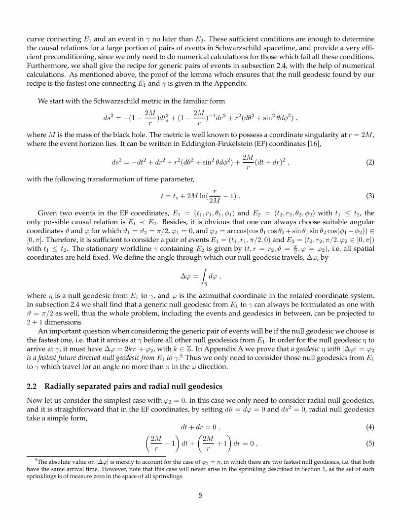
Figure 1: Illustration of the timelike worldline γ, on which all spatial coordinates (including r) are constant,and two null geodesics from E1 to γ.
t1 < t2, the only possible causal relation between them is that E1 ≺ E2, which means that there is a future-directed causal curve from E1 to E2. Imagine a bunch of light rays (null geodesics) B, emanating from E1, andE2 represents a particular moment t2 in the world line γ of a stationary observer. If the world line of any nullgeodesics in B, which is a null geodesic, meets γ at t ≤ t2, then we can conclude that they are causally-related.On the other hand, if any null geodesic emanating from E1 can only reach γ at t > t2, then E1 and E2 must becausally unrelated to each other. See Fig. 1 for an illustration. That this is true can be seen by proposition 2.20of [15], which states if A ∈ J−(B) but A 6∈ I−(B), then there must exist a future-directed null geodesic fromA to B. This tells us that the earliest future-directed causal curve must be a null geodesic, but since any nullgeodesic has failed to reach γ early enough for a causal relation between the two events, then the conclusion isthat there is no causal relation between them.
We will prove in Appendix A that our procedure always considers the fastest3 geodesic from E1 to γ, so thearrival time t at γ of that geodesic will be sufficient to determine if E1 and E2 are causally related. If we findthat even this null geodesic meets γ later than t2, we can say for sure that there is no way for these two eventsto be connected by any future directed causal curve.
After this brief introduction, we discuss in the next subsection the particular simple case where E1 and E2
are only radially separated, with no angular separation, so all we need to consider are radial geodesics. Formore generic pairs of events, we must consider the full three dimensional case,4 which is too complicated for acomplete analytic solution. However, before incorporating a numerical treatment for the generic case, in sub-section 2.3 we find two simple sufficient conditions for two events to be causally unrelated to each other. Oneuses a bound given by radial null geodesics, and the other by purely angular components. Furthermore, thereis also a sufficient condition for two events to have causal relation, which is the existence of a composed null
3By ‘fastest’ we mean the geodesic with the earliest arrival time, as given by the (EF) time coordinate.4Given two events in Schwarzschild spacetime, is is always possible to rotate the coordinates so that they both lie in the equatorial
plane, as explained below.
4
curve connecting E1 and an event in γ no later than E2. These sufficient conditions are enough to determinethe causal relations for a large portion of pairs of events in Schwarzschild spacetime, and provide a very effi-cient preconditioning, since we only need to do numerical calculations for those which fail all these conditions.Furthermore, we shall give the recipe for generic pairs of events in subsection 2.4, with the help of numericalcalculations. As mentioned above, the proof of the lemma which ensures that the null geodesic found by ourrecipe is the fastest one connecting E1 and γ is given in the Appendix.
We start with the Schwarzschild metric in the familiar form
ds2 = −(1− 2M
r)dt2s + (1− 2M
r)−1dr2 + r2(dθ2 + sin2 θdφ2) ,
where M is the mass of the black hole. The metric is well known to possess a coordinate singularity at r = 2M ,where the event horizon lies. It can be written in Eddington-Finkelstein (EF) coordinates [16],
ds2 = −dt2 + dr2 + r2(dθ2 + sin2 θdφ2) +2M
r(dt+ dr)2 , (2)
with the following transformation of time parameter,
t = ts + 2M ln(r
2M− 1) . (3)
Given two events in the EF coordinates, E1 = (t1, r1, θ1, φ1) and E2 = (t2, r2, θ2, φ2) with t1 ≤ t2, theonly possible causal relation is E1 ≺ E2. Besides, it is obvious that one can always choose suitable angularcoordinates ϑ and ϕ for which ϑ1 = ϑ2 = π/2, ϕ1 = 0, and ϕ2 = arccos(cos θ1 cos θ2+sin θ1 sin θ2 cos(φ1−φ2)) ∈[0, π]. Therefore, it is sufficient to consider a pair of events E1 = (t1, r1, π/2, 0) and E2 = (t2, r2, π/2, ϕ2 ∈ [0, π])with t1 ≤ t2. The stationary worldline γ containing E2 is given by (t, r = r2, ϑ = π
2, ϕ = ϕ2), i.e. all spatial
coordinates are held fixed. We define the angle through which our null geodesic travels, ∆ϕ, by
∆ϕ =
∫
ηdϕ ,
where η is a null geodesic from E1 to γ, and ϕ is the azimuthal coordinate in the rotated coordinate system.In subsection 2.4 we shall find that a generic null geodesic from E1 to γ can always be formulated as one withϑ = π/2 as well, thus the whole problem, including the events and geodesics in between, can be projected to2 + 1 dimensions.
An important question when considering the generic pair of events will be if the null geodesic we choose isthe fastest one, i.e. that it arrives at γ before all other null geodesics from E1. In order for the null geodesic η toarrive at γ, it must have ∆ϕ = 2kπ + ϕ2, with k ∈ Z. In Appendix A we prove that a geodesic η with |∆ϕ| = ϕ2
is a fastest future directed null geodesic from E1 to γ.5 Thus we only need to consider those null geodesics from E1
to γ which travel for an angle no more than π in the ϕ direction.
2.2 Radially separated pairs and radial null geodesics
Now let us consider the simplest case with ϕ2 = 0. In this case we only need to consider radial null geodesics,and it is straightforward that in the EF coordinates, by setting dϑ = dϕ = 0 and ds2 = 0, radial null geodesicstake a simple form,
dt+ dr = 0 , (4)(
2M
r− 1
)
dt+
(
2M
r+ 1
)
dr = 0 , (5)
5The absolute value on |∆ϕ| is merely to account for the case of ϕ2 = π, in which there are two fastest null geodesics, i.e. that bothhave the same arrival time. However, note that this case will never arise in the sprinkling described in Section 1, as the set of suchsprinklings is of measure zero in the space of all sprinklings.
5
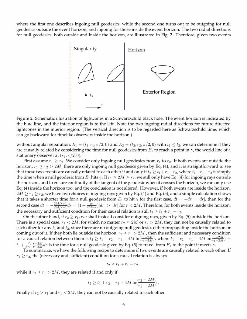
where the first one describes ingoing null geodesics, while the second one turns out to be outgoing for nullgeodesics outside the event horizon, and ingoing for those inside the event horizon. The two radial directionsfor null geodesics, both outside and inside the horizon, are illustrated in Fig. 2. Therefore, given two events
HorizonSingularity
Exterior RegionPSfrag replacements ts
r
Figure 2: Schematic illustration of lightcones in a Schwarzschild black hole. The event horizon is indicated bythe blue line, and the interior region is to the left. Note the two ingoing radial directions for future directedlightcones in the interior region. (The vertical direction is to be regarded here as Schwarzschild time, whichcan go backward for timelike observers inside the horizon.)
without angular separation, E1 = (t1, r1, π/2, 0) and E2 = (t2, r2, π/2, 0) with t1 ≤ t2, we can determine if theyare causally related by considering the time for null geodesics from E1 to reach a point in γ, the world line of astationary observer at (r2, π/2, 0).
First assume r1 ≥ r2. We consider only ingoing null geodesics from r1 to r2. If both events are outside thehorizon, r1 ≥ r2 > 2M , there are only ingoing null geodesics given by Eq. (4), and it is straightforward to seethat these two events are causally related to each other if and only if t2 ≥ t1+r1−r2, where t1+r1−r2 is simplythe time when a null geodesic from E1 hits γ. If r1 ≥ 2M ≥ r2, we still only have Eq. (4) for ingoing rays outsidethe horizon, and to ensure continuity of the tangent of the geodesic when it crosses the horizon, we can only useEq. (4) inside the horizon too, and the conclusion is not altered. However, if both events are inside the horizon,2M ≥ r1 ≥ r2, we have two choices of ingoing rays given by Eq. (4) and Eq. (5), and a simple calculation showsthat it takes a shorter time for a null geodesic from E1 to hit γ for the first case, dt = −dr = |dr|, than for the
second case dt = −2M/r+1
2M/r−1dr = (1+ 2r
2M−r )|dr| > |dr| for r < 2M . Therefore, for both events inside the horizon,
the necessary and sufficient condition for their causal relation is still t2 ≥ t1 + r1 − r2.On the other hand, if r2 ≥ r1, we shall instead consider outgoing rays, given by Eq. (5) outside the horizon.
There is a special case, r1 < 2M , for which no matter r2 ≤ 2M or r2 > 2M , they can not be causally related toeach other for any t1 and t2, since there are no outgoing null geodesics either propagating inside the horizon orcoming out of it. If they both lie outside the horizon, r2 ≥ r1 > 2M , then the sufficient and necessary conditionfor a causal relation between them is t2 ≥ t1 + r2 − r1 + 4M ln( r2−2M
r+2Mr−2M dr is the time for a null geodesic given by Eq. (5) to travel from E1 to the point it meets γ.
To summarize, we have the following recipe to determine if two events are causally related to each other. Ifr1 ≥ r2, the (necessary and sufficient) condition for a causal relation is always
t2 ≥ t1 + r1 − r2 ,
while if r2 ≥ r1 > 2M , they are related if and only if
t2 ≥ t1 + r2 − r1 + 4M ln(r2 − 2M
r1 − 2M) .
Finally if r2 > r1 and r1 < 2M , they can not be causally related to each other.
6
2.3 Sufficient conditions for causally related and unrelated pairs
Since in practice we are interested in computing the causal relations between many pairs of events, it is useful toderive bounds that allow one to decide whether the events are related quickly, based on simple criteria, withouthaving to perform any numerical integrations. In this section we derive such bounds, which are sufficient todetermine that the two events are unrelated (section 2.3.1) or related (section 2.3.2).
2.3.1 Spacelike bounds
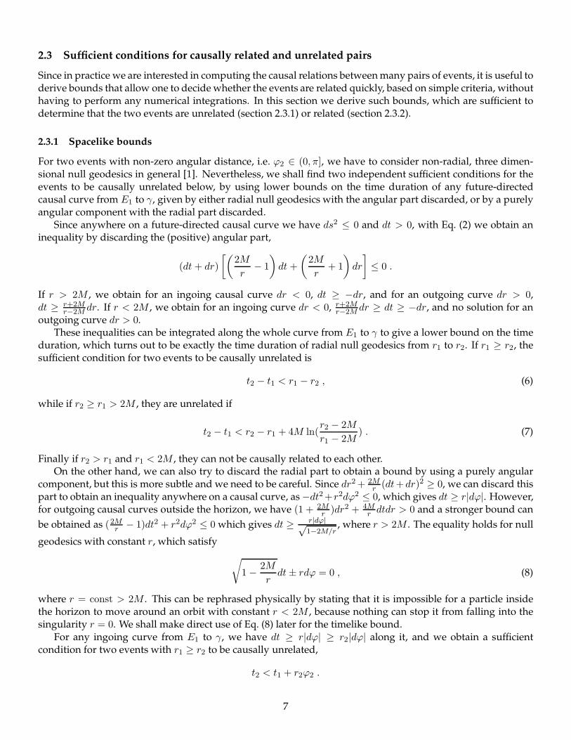
For two events with non-zero angular distance, i.e. ϕ2 ∈ (0, π], we have to consider non-radial, three dimen-sional null geodesics in general [1]. Nevertheless, we shall find two independent sufficient conditions for theevents to be causally unrelated below, by using lower bounds on the time duration of any future-directedcausal curve from E1 to γ, given by either radial null geodesics with the angular part discarded, or by a purelyangular component with the radial part discarded.
Since anywhere on a future-directed causal curve we have ds2 ≤ 0 and dt > 0, with Eq. (2) we obtain aninequality by discarding the (positive) angular part,
(dt+ dr)
[(
2M
r− 1
)
dt+
(
2M
r+ 1
)
dr
]
≤ 0 .
If r > 2M , we obtain for an ingoing causal curve dr < 0, dt ≥ −dr, and for an outgoing curve dr > 0,dt ≥ r+2M
r−2M dr. If r < 2M , we obtain for an ingoing curve dr < 0, r+2Mr−2M dr ≥ dt ≥ −dr, and no solution for an
outgoing curve dr > 0.These inequalities can be integrated along the whole curve from E1 to γ to give a lower bound on the time
duration, which turns out to be exactly the time duration of radial null geodesics from r1 to r2. If r1 ≥ r2, thesufficient condition for two events to be causally unrelated is
t2 − t1 < r1 − r2 , (6)
while if r2 ≥ r1 > 2M , they are unrelated if
t2 − t1 < r2 − r1 + 4M ln(r2 − 2M
r1 − 2M) . (7)
Finally if r2 > r1 and r1 < 2M , they can not be causally related to each other.On the other hand, we can also try to discard the radial part to obtain a bound by using a purely angular
component, but this is more subtle and we need to be careful. Since dr2+ 2Mr (dt+ dr)2 ≥ 0, we can discard this
part to obtain an inequality anywhere on a causal curve, as −dt2+r2dϕ2 ≤ 0, which gives dt ≥ r|dϕ|. However,for outgoing causal curves outside the horizon, we have (1 + 2M
r )dr2 + 4Mr dtdr > 0 and a stronger bound can
be obtained as (2Mr − 1)dt2 + r2dϕ2 ≤ 0 which gives dt ≥ r|dϕ|√1−2M/r
, where r > 2M . The equality holds for null
geodesics with constant r, which satisfy
√
1− 2M
rdt± rdϕ = 0 , (8)
where r = const > 2M . This can be rephrased physically by stating that it is impossible for a particle insidethe horizon to move around an orbit with constant r < 2M , because nothing can stop it from falling into thesingularity r = 0. We shall make direct use of Eq. (8) later for the timelike bound.
For any ingoing curve from E1 to γ, we have dt ≥ r|dϕ| ≥ r2|dϕ| along it, and we obtain a sufficientcondition for two events with r1 ≥ r2 to be causally unrelated,
t2 < t1 + r2ϕ2 .
7
For any outgoing curves from E1 to γ, we have dt ≥ r|dϕ|√1−2M/r
along it, and we need to find out the minimum
of f(r) = r√1−2M/r
in the range 2M < r1 ≤ r ≤ r2. It is straightforward to obtain
f ′(r) =1− 3M/r
(1− 2M/r)3/2,
from which the location of the minimum can be determined to be r0 = r1 for 3M ≤ r1 ≤ r2, r0 = 3M forr1 < 3M < r2, and r0 = r2 for r1 ≤ r2 ≤ 3M .
Therefore we have dt ≥ r0|dϕ|√1−2M/r0
along the curve and we obtain a sufficient condition for two events with
2M < r1 ≤ r2 to be causally unrelated,t2 − t1 < f(r0)ϕ2 . (9)
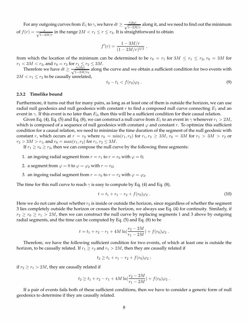
2.3.2 Timelike bound
Furthermore, it turns out that for many pairs, as long as at least one of them is outside the horizon, we can useradial null geodesics and null geodesics with constant r to find a composed null curve connecting E1 and anevent in γ. If this event is no later than E2, then this will be a sufficient condition for their causal relation.
Given Eq. (4), Eq. (5) and Eq. (8), we can construct a null curve from E1 to an event in γ whenever r1 > 2M ,which is composed of a sequence of null geodesics with constant ϕ and constant r. To optimize this sufficientcondition for a causal relation, we need to minimize the time duration of the segment of the null geodesic withconstant r, which occurs at r = r0 where r0 = min(r1, r2) for r1, r2 ≥ 3M , r0 = 3M for r1 > 3M > r2 orr2 > 3M > r1, and r0 = max(r1, r2) for r1, r2 ≤ 3M .
If r1 ≥ r0 ≥ r2, then we can compose the null curve by the following three segments:
1. an ingoing radial segment from r = r1 to r = r0 with ϕ = 0;
2. a segment from ϕ = 0 to ϕ = ϕ2 with r = r0;
3. an ingoing radial segment from r = r0 to r = r2 with ϕ = ϕ2.
The time for this null curve to reach γ is easy to compute by Eq. (4) and Eq. (8),
t = t1 + r1 − r2 + f(r0)ϕ2 . (10)
Here we do not care about whether r2 is inside or outside the horizon, since regardless of whether the segment3 lies completely outside the horizon or crosses the horizon, we always use Eq. (4) for continuity. Similarly, ifr2 ≥ r0 ≥ r1 > 2M , then we can construct the null curve by replacing segments 1 and 3 above by outgoingradial segments, and the time can be computed by Eq. (5) and Eq. (8) to be
t = t1 + r2 − r1 + 4M ln(r2 − 2M
r1 − 2M) + f(r0)ϕ2 .
Therefore, we have the following sufficient condition for two events, of which at least one is outside thehorizon, to be causally related. If r1 ≥ r2 and r1 > 2M , then they are causally related if
t2 ≥ t1 + r1 − r2 + f(r0)ϕ2 ;
if r2 ≥ r1 > 2M , they are causally related if
t2 ≥ t1 + r2 − r1 + 4M ln(r2 − 2M
r1 − 2M) + f(r0)ϕ2 .
If a pair of events fails both of these sufficient conditions, then we have to consider a generic form of nullgeodesics to determine if they are causally related.
8
2.4 Generic pairs of events and null geodesics
The most generic null geodesics in Schwarzschild spacetime have the following form [1],
ptdt
dτ− pr
dr
dτ− pθ
dθ
dτ− pφ
dφ
dτ= 0 ,
where τ is an affine parameter, and pt, pφ are constants,
pt = (1− 2M
r)dtsdτ
= E ,
pφ = r2 sin2 θdφ
dτ= L ,
and pφ satisfies
d(r2 dθdτ )
dτ= r2 sin θ cos θ(
dφ
dτ)2 .
If we choose ϑ = π/2 at the moment when dϑdτ = 0, we get also d2ϑ
dτ2= 0 at this moment, which implies ϑ = π/2
all along the geodesic. Therefore a general null geodesic can be described in the plane ϑ = π/2, which alsosimplifies its equations to
(dr
dτ)2 +
L2
r2(1− 2M
r) = E2 , (11)
where E and L denote the constant energy and angular momentum of the massless particle,
(1− 2M
r)dtsdτ
= E ,
dϕ
dτ=
L
r2. (12)
The energy is expressed in terms of the Schwarzschild time parameter ts.The full set of Eq. (11) and Eq. (12), combined with initial values of t, r and ϕ, as well as E and L, can
uniquely determine a null geodesic in Schwarzschild spacetime. However, since we only want to obtain rela-tions between t, r and ϕ without the affine parameter τ , it is convenient to consider r as a function of ϕ and usea new variable u = 1/r. We then obtain from Eq. (11),
(du
dϕ)2 = 2Mu3 − u2 + c2 ,
or equivalently,dϕ
du= ±(2Mu3 − u2 + c2)−1/2 , (13)
where + corresponds to dϕ/du > 0, − corresponds to dϕ/du < 0, and c = E/L for L 6= 0. The case of L = 0,which corresponds to radial null geodesics, has been discussed in Subsection 2.2. It turns out that, for L 6= 0,the geodesic depends on E and L only through their ratio c. Using Eq. (3) and Eq. (12), we can further obtain
dt
dϕ=
cr2
1− 2M/r+
dr/dϕ
r/2M − 1,
which can be simplified by using the new variable u = 1/r and Eq. (13) as
dt
dϕ=
c∓ 2Mu√2Mu3 − u2 + c2
u2 − 2Mu3. (14)
9
Alternatively, we can put it into an equation involving only t and u,
dt
du=
±c(2Mu3 − u2 + c2)−1/2 − 2Mu
u2 − 2Mu3, (15)
where, as mentioned before, + corresponds to dϕ/du > 0, − corresponds to dϕ/du < 0. Eq. (13) and Eq. (14),or equivalently Eq. (13) and Eq. (15) is a full set of equations for generic null geodesics with non-zero angularmomenta.
Now given E1 and E2 which do not satisfy any of the sufficient conditions in Subsection 2.3, we have to dothe following numerical calculation to see if they are causally related to each other. For any c we can integrateEq. (13) from ϕ1 = 0, u1 = 1/r1 to u2 = 1/r2, and get some value ϕ′
2. By choosing a suitable c0, we can makeϕ′2 = ϕ2 which means that the null geodesic with c0 hits γ from E1. Then we can use c0 in Eq. (15), and integrate
it from u1, t1 to u2 and get some value t. If t ≤ t2, then they are definitely causally related. If t > t2, accordingto the lemma of Section 2.1, they must be causally unrelated.
3 Results
3.1 Causal Relations
We sprinkle into a region of Schwarzschild spacetime, which is bounded by 0 ≤ r ≤ rmax and 0 ≤ t ≤ tmax. SeeAppendix B.1 for details on how this is done. It is important to note that in this section we use the unrotatedcoordinates, so θ is not restricted to π
2, and use coordinates such that M = 1. By ‘equatorial plane’, we simply
mean that θ = π2
.Nine events selected from a region of Schwarzschild with rmax = 3, tmax = 8, are shown in Table 1.6
Table 1: Nine events in Schwarzschild spacetime, specified by their Eddington-Finkelstein coordinates.
Our task is to decide, for each pair of events (E1, E2) (with E1 having an earlier EF time coordinate thanE2), whether they are causally related or not. To do this we perform the following algorithm:
1. Is E1 is behind the horizon and r2 > r1? If so they are unrelated.
2. Change the angular coordinates so that both lie on the equatorial plane, and restrict attention to nullgeodesics which traverse an azimuthal angle ≤ π on their trip from E1 to a stationary worldline γ con-taining E2.
3. Is the EF time separation of the events less than the angular or radial spacelike bounds? If so they areunrelated.
6We chose rmax = 3 to get roughly the same number of interior and exterior events, and tmax = 8 to be roughly half the circumfer-ence of a circle at r = 3. Note that r = 3 corresponds to the innermost circular orbit (which is therefore lightlike).
10
4. Is the EF time separation greater than the timelike bound? If so they are related.
5. If neither sufficient condition is satisfied, then we must numerically compute the value of (E/L)2 whichwill send a null geodesic from E1 to γ. Armed with this value, we compute the elapsed coordinate timealong this geodesic, and decide if it arrives before or after the event E2.
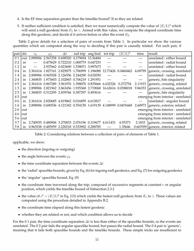
Table 2 gives details for a selection of pairs of events from Table 1. In particular we show the variousquantities which are computed along the way to deciding if this pair is causally related. For each pair, if
pair dir r0 ϕ2 ∆t rad trip ang bnd tot trip (E/L)2 time result
0 1 out 2.898906 2.567258 0.698520 4.179694 13.36484 — — — unrelated : either bound0 2 in — 0.475629 0.722210 1.000779 0.647253 — — — unrelated : radial bound1 2 in — 2.937662 0.023690 1.538071 3.997673 — — — unrelated : either bound0 4 in 2.361614 1.827161 2.825075 1.706999 1.196088 12.73426 0.0460462 4.69799 generic, crossing, unrelated1 4 in 2.898906 0.965528 2.126556 2.244290 0.632050 — — — unrelated : radial bound2 4 in 1.360835 1.973603 2.102865 0.706219 1.291951 — — — generic, hits singularity0 5 in 2.361614 0.867289 3.561976 1.398076 0.835666 6.632326 0.272754 2.11915 generic, crossing, related1 5 in 2.898906 2.821962 2.863456 1.935368 2.719068 16.62616 0.0388018 9.86353 generic, crossing, unrelated2 5 in 1.360835 0.512295 2.839766 0.397297 0.493616 — — — generic, hits singularity4 5 out emerging from interior : unrelated0 6 in 2.361614 2.820685 4.819862 0.016859 6.613817 — — — unrelated : angular bound1 6 in 2.898906 0.690536 4.121342 0.554150 1.619139 4.148999 0.0476468 2.60973 generic, exterior, related2 6 out emerging from interior : unrelated4 6 out emerging from interior : unrelated5 6 out emerging from interior : unrelated3 7 in 2.740935 0.480906 3.270833 2.076196 0.319677 4.611431 4.55373 2.1833 generic, crossing, related5 8 in 0.963538 0.485959 2.220218 0.533902 0.208785 — 1.35646 0.667059 generic, interior, related
Table 2: Considering relations between a collection of pairs of elements of Table 1.
applicable, we show:
• the direction (ingoing or outgoing)
• the angle between the events ϕ2
• the time coordinate separation between the events ∆t
• the ‘radial’ spacelike bounds, given by Eq. (6) for ingoing null geodesics, and Eq. (7) for outgoing geodesics
• the ‘angular’ spacelike bound, Eq. (9)
• the coordinate time traversed along the trip, composed of successive segments at constant r or angularposition, which yields the timelike bound of Subsection 2.3.2
• the value of c2 = (E/L)2 in Eq. (13) which yields the fastest null geodesic from E1 to γ. These values arecomputed using the procedure detailed in Appendix B.2.
• the coordinate time elapsed along this fastest geodesic
• whether they are related or not, and which condition allows us to decide
For the 0 1 pair, the time coordinate separation ∆t is less than either of the spacelike bounds, so the events areunrelated. The 0 2 pair fails the angular spacelike bound, but passes the radial bound. The 0 4 pair is ‘generic’,meaning that it fails both spacelike bounds and the timelike bounds. These simple tricks are insufficient to
11
determine if the events are related, so we must integrate Eq. (13) to locate the fastest null geodesic from event 0to the γ containing event 4. This geodesic crosses the horizon, but does not arrive at γ in time for the events tobe related (since the ‘time’ in the last column is larger than the ‘available time’ ∆t). The 2 4 pair fails the radialspacelike bound. The radial and timelike bounds fail because the pair is inside the horizon, for which there isno timelike, constant-r trajectory. Integrating (13), with c2 ≡ (E/L)2 = 0, gives only ϕ = 0.721811, which isnot enough to reach γ. All null geodesics will hit the singularity before reaching the θ2 = 0.11664, φ2 = 0.11664worldline. The 2 5 pair meets a similar fate: there are no future directed null geodesics from event 2 whichreach θ2 = 2.33727, φ2 = 1.38169 before falling into the singularity. The 0 5 pair fails all bounds, and thus isgeneric. This time, however, the null geodesic does reach γ before event 5. The 4 5 pair represents an attemptto ‘escape from the interior’, in the sense that event 4 is inside the horizon, and event 5 is at a larger radius than4. Even though event 5 is also inside the horizon, there are no causal curves inside the horizon which extendto larger radii. Events 0 and 6 are at almost the same radius, but at very different angular positions. Thus theangular bound is useful in deducing that they are unrelated, without having to integrate any geodesics. Events1 and 6 are an example of a generic pair which are both outside of the horizon. They happen to be related.The pairs 2 6, 4 6, and 5 6 suffer the same fate as 4 5. This time they are even attempting to escape across thehorizon. The 5 8 pair is generic and completely inside the horizon. This time there are causal curves whichreach γ from event 5, and the events end up being related.
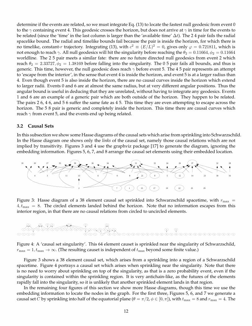
3.2 Causal Sets
In this subsection we show some Hasse diagrams of the causal sets which arise from sprinkling into Schwarzschild.In the Hasse diagram one shows only the links of the causal set, namely those causal relations which are notimplied by transitivity. Figures 3 and 4 use the graphviz package [17] to generate the diagram, ignoring theembedding information. Figures 5, 6, 7, and 8 arrange the causal set elements using their embedded location.
0
30 31
12
13
20
21
3436
3
27 35
4
10
5
24 2633 37
6
7
8 911 12 14
15
16
2832
17
18
19 22
23
25 29
Figure 3: Hasse diagram of a 38 element causal set sprinkled into Schwarzschild spacetime, with rmax =4, tmax = 8. The circled elements landed behind the horizon. Note that no information escapes from thisinterior region, in that there are no causal relations from circled to uncircled elements.
0 1 2
3
61
4 5 6
1432 47 51
52
7
8
26 63
9 10 11 1213
18 36
33
15 16 17 1920 21 22
6023
2462
25
27 28
29
30 3134
35 37 38
39 40
41
42 43
44 45 46
48 49
50
53 54 55 56 57
58 59
Figure 4: A ‘causal set singularity’. This 64 element causet is sprinkled near the singularity of Schwarzschild,rmax = 1, tmax → ∞. (The resulting causet is independent of tmax beyond some finite value.)
Figure 3 shows a 38 element causal set, which arises from a sprinkling into a region of a Schwarzschildspacetime. Figure 4 portrays a causal set which arises when sprinkling near the singularity. Note that thereis no need to worry about sprinkling on top of the singularity, as that is a zero probability event, even if thesingularity is contained within the sprinkling region. It is very antichain-like, as the futures of the elementsrapidly fall into the singularity, so it is unlikely that another sprinkled element lands in that region.
In the remaining four figures of this section we show more Hasse diagrams, though this time we use theembedding information to locate the nodes in the graph. For the first three, Figures 5, 6, and 7 we generate acausal set C by sprinkling into half of the equatorial plane (θ = π/2, φ ∈ [0, π]), with tmax = 8 and rmax = 4. The
12
-4-3
-2-1
0 1
2 3
4-4-3
-2-1
0 1
2 3
4
0 1 2 3 4 5 6 7 8
t
xy
t
Figure 5: Hasse diagram of a causal set C which arises from sprinkling 91 elements into the half equatorialplane. Elements sprinkled behind the horizon appear blue, while those outside are green.
13
-3 -2 -1 0 1 2 3 0
0.5
1
1.5
2
2.5
3 0 1 2 3 4 5 6 7 8t
x
y
t
Figure 6: The same 91 element causal set C as viewed from the ‘top’ (t → +∞, look into the past direction).The blue ‘half disk’ corresponds to the black hole interior.
14
0 0.5 1 1.5 2 2.5 3 3.5 4 0
0.5 1
1.5 2
2.5 3
3.5
0 1 2 3 4 5 6 7 8
t
r
t
PSfrag replacements
φ
Figure 7: The sprinkled 91 element causal set C , this time plotting r against φ interpreted as Cartesian co-ordinates, rather than polar coordinates. The blue region on the left corresponds to the interior of the blackhole.
15
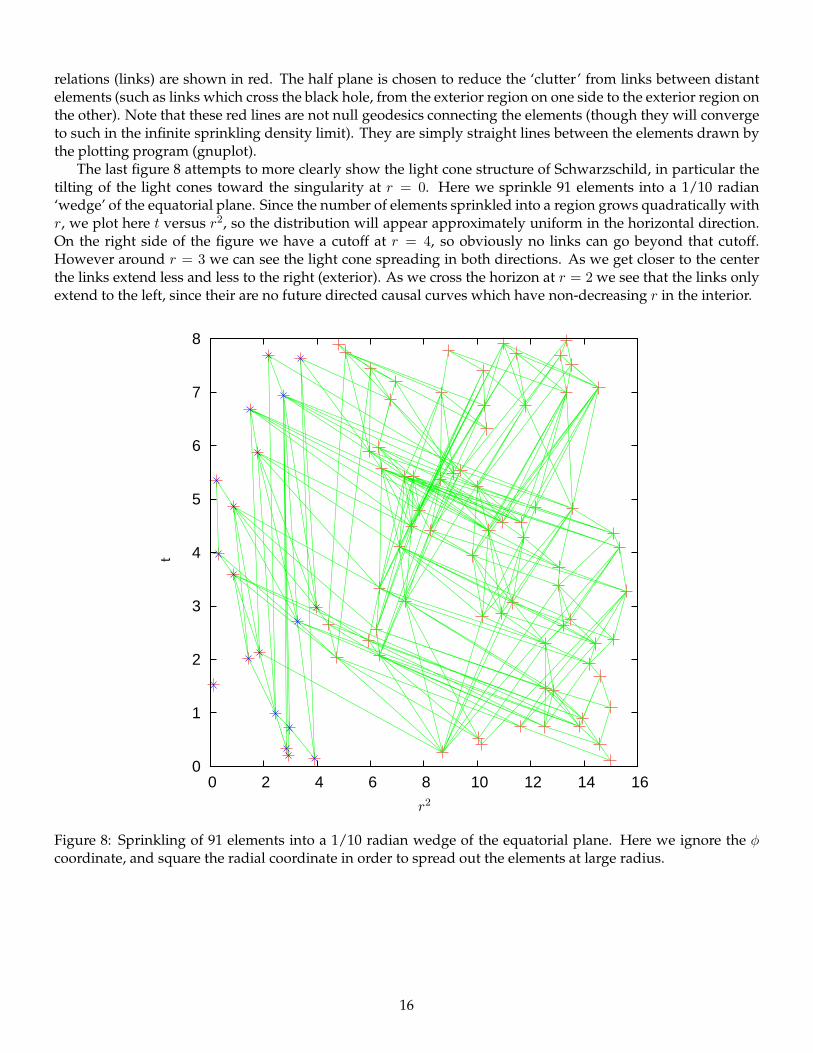
relations (links) are shown in red. The half plane is chosen to reduce the ‘clutter’ from links between distantelements (such as links which cross the black hole, from the exterior region on one side to the exterior region onthe other). Note that these red lines are not null geodesics connecting the elements (though they will convergeto such in the infinite sprinkling density limit). They are simply straight lines between the elements drawn bythe plotting program (gnuplot).
The last figure 8 attempts to more clearly show the light cone structure of Schwarzschild, in particular thetilting of the light cones toward the singularity at r = 0. Here we sprinkle 91 elements into a 1/10 radian‘wedge’ of the equatorial plane. Since the number of elements sprinkled into a region grows quadratically withr, we plot here t versus r2, so the distribution will appear approximately uniform in the horizontal direction.On the right side of the figure we have a cutoff at r = 4, so obviously no links can go beyond that cutoff.However around r = 3 we can see the light cone spreading in both directions. As we get closer to the centerthe links extend less and less to the right (exterior). As we cross the horizon at r = 2 we see that the links onlyextend to the left, since their are no future directed causal curves which have non-decreasing r in the interior.
0
1
2
3
4
5
6
7
8
0 2 4 6 8 10 12 14 16PSfrag replacements
t
r2
Figure 8: Sprinkling of 91 elements into a 1/10 radian wedge of the equatorial plane. Here we ignore the φcoordinate, and square the radial coordinate in order to spread out the elements at large radius.
16
4 Conclusion and discussion
We have described an algorithm to determine if two events are causally related in Schwarzschild spacetime.It involves first checking a number of sufficient conditions, to see if these are able to determine whether theyare related, without resorting to a time consuming numerical integration. If none of these are satisfied then welocate a future directed null geodesic which leads from the earlier event to a worldline containing the later, andintegrate the elapsed EF time along the geodesic to determine if the pair is related.
We then wrote a ‘thorn’ (module) within the Cactus framework with sprinkles events into a region ofSchwarzschild, and use this algorithm to deduce the causal relations between every pair of events. This proce-dure yields a causal set which ‘faithfully embeds’ into a Schwarzschild black hole spacetime.
It should not be difficult to generalize this prescription to other black hole spacetimes, such as Reissner-Nordstrom or Kerr. In order to describe the closed timelike curves in interior regions one may generalize thedefinition of the causal set slightly, replacing the irreflexive condition with reflexivity, so one ends up witha transitive directed graph. In addition one can consider other conformally curved spacetimes, such as thek = ±1 Friedman-Robertson-Walker universes.
This work is a good starting point for one to address a wide array of questions within the causal set program,which previously were inaccessible. On one hand it will allow one to easily investigate many kinematicalquestions with regard to the so-called ‘Hauptvermutung’ of causal sets, which conjectures that if one has acausal set which is likely to arise from sprinkling into two separate spacetimes, then those spacetimes mustbe approximately isometric. To date, all results regarding to how to deduce properties of an approximatingcontinuum from a causal set consider only conformally flat geometries. Now one will be able to test suchconstructs on a much wider class of geometries.
Another important application is towards our understanding of black hole thermodynamics. The funda-mental discreteness of causal sets gives us a possible way to characterize the degrees of freedom which giverise to black hole entropy. We are now in a position to repeat the analysis of the link counting and its gen-eralizations [12], for the full 4d Schwarzschild geometry. As argued by Dou and Sorkin, this may provideaccess to the fundamental length scale of quantum gravity, since entropy, as a pure number, is not subject torenormalization.
Finally, a long standing question in semi-classical gravity is the trans-Planckian problem, that the Hawkingradiation emanating from a black hole horizon, at late times (after the black hole forms), arises from modes offrequency much greater than the Planck scale [18]. If spacetime is discrete at this scale, then one may expectthat such trans-Planckian modes cannot exist. How then is Hawking radiation possible, in such a discretesetting? Important groundwork on the dynamics of scalar fields on a background causal set has recently beenlaid [19, 20, 21]. Now that we can construct causal sets which correspond to a full four dimensional black hole,it may be possible to address this question within the causal set approach.
Acknowledgments
We are extremely grateful to Joseph Samuel and Rafael Sorkin for illuminating discussions on the behaviorof null geodesics and their relation to causal structure. SH also thanks Hongbao Zhang for many helpfuldiscussions and comments.
This research was supported by the Perimeter Institute for Theoretical Physics. Research at Perimeter In-stitute is supported by the Government of Canada through Industry Canada and by the Province of Ontariothrough the Ministry of Research & Innovation. SH was supported by NFSC grants 10235040 and 10421003.
SH thanks the Perimeter Institute for hospitality while this work was carried out.
17
A Appendix: Proof of the proposition
In this section, we want to prove the following proposition. Given two events E1 and E2 in Schwarzschildspacetime, with t1 < t2, and E2 representing the moment t2 on the world line γ of a stationary observer, thenull geodesic with |∆ϕ| = ϕ2 is the fastest one (arrives at the earliest time in EF coordinates) for all future-directed null geodesics from E1 to γ.
It is clear that the fastest geodesic will have the least elapsed time. Thus from Eq. (15), we wish to minimizethe integral
∆t =
∫ u2
u1
±c(2Mu3 − u2 + c2)−1/2 − 2Mu
u2 − 2Mu3du (16)
along the geodesic. Since dϕ is clearly nonnegative, the sign in front of c will be positive for ingoing geodesics(du > 0) and negative for outgoing geodesics (du < 0). Given E1 and E2 (and thus γ), different null geodesicsare given by different values of c, and it is straightforward to see from Eq. (16) that in every case for larger c,∆t gets smaller. Therefore, the fastest null geodesic from E1 to γ must have the largest possible c to reach γ,which, by Eq. ( 13), has the smallest possible |∆ϕ| = ϕ2.7
B Numerical Details
B.1 Sprinkling into Schwarzschild Spacetime
In implementing these ideas on a computer, the first task is to randomly select events in spacetime, with adensity proportional to the spacetime volume factor
√−g = r√
r2 + 12M2 sin θ . (17)
Because of the simple product form of this expression, we can break up the sprinkling into an angular piece,a temporal piece, and a radial piece. For the uniform sprinkling of the angular coordinates, on a 2-sphere, wefollow the procedure described in Section 5.2 of [22]. For the temporal sprinkling, since the volume element isindependent of t, we can select its values uniformly at random.
The sprinkling in the radial direction must be performed such that it yields the distribution of Eq. (17)(ignoring the θ dependence; this is accounted for above). This is achieved by the following general method(derived from [23]). To sprinkle a coordinate x between the bounds a ≤ x ≤ b such that it has distribution f(x),compute the indefinite integral
I(x) =1
N
∫ x
af(x′)dx′ , (18)
where the constant normalization factor is
N =
∫ b
af(x′)dx′ .
Now invert Eq. (18) to get x as a function of I . This expression, where I is a random variable distributeduniformly in the unit interval [0, 1], will be distributed according to f(x). Of course this method only worksif f(x) is integrable and its integral is invertible. In our case f(r) = r
√r2 + 12M2, and the expression is
√
(3NI + (a2 + 12M2)3/2)2/3 − 12M2. 8
7As mentioned earlier, for ϕ2 < π, there is only one fastest null geodesic with the largest c to make ∆ϕ = ϕ2; while for ϕ2 = π,there are in fact two fastest null geodesics with ∆ϕ = ±π but the same c and ∆t.
8In fact the angular sprinkling is of this type as well. With f(θ) = sin θ the expression is arccos(2I − 1). The φ coordinate isdistributed uniformly in [0, 2π].
18
B.2 Determining the Causal Relations
Once equipped with a collection of events in Schwarzschild, we can sort them by their time coordinate, and thenconsider each sorted pair in turn. The first task is to check the sufficient conditions described in Subsection 2.3.This is relatively straightforward; numerous examples are given in Subsection 3.1. If the pair fails all availablesufficient conditions, then it is a ‘generic pair’, and we must integrate null geodesics as described in Subsection2.4.
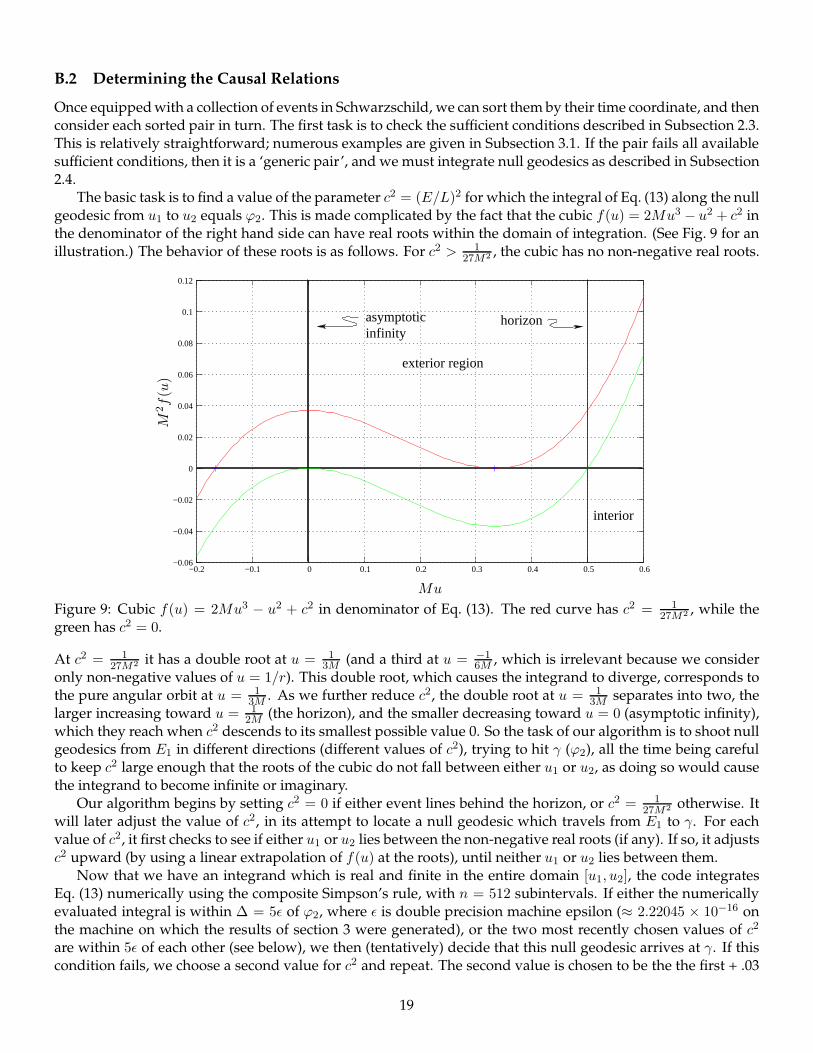
The basic task is to find a value of the parameter c2 = (E/L)2 for which the integral of Eq. (13) along the nullgeodesic from u1 to u2 equals ϕ2. This is made complicated by the fact that the cubic f(u) = 2Mu3 − u2 + c2 inthe denominator of the right hand side can have real roots within the domain of integration. (See Fig. 9 for anillustration.) The behavior of these roots is as follows. For c2 > 1
27M2 , the cubic has no non-negative real roots.
infinityasymptotic
interior
horizon
exterior region
−0.06
−0.04
−0.02
0
0.02
0.04
0.06
0.08
0.1
0.12
−0.2 −0.1 0 0.1 0.2 0.3 0.4 0.5 0.6
PSfrag replacements
Mu
M2f(u)
Figure 9: Cubic f(u) = 2Mu3 − u2 + c2 in denominator of Eq. (13). The red curve has c2 = 1
27M2 , while thegreen has c2 = 0.
At c2 = 1
27M2 it has a double root at u = 1
3M (and a third at u = −1
6M , which is irrelevant because we consideronly non-negative values of u = 1/r). This double root, which causes the integrand to diverge, corresponds tothe pure angular orbit at u = 1
3M . As we further reduce c2, the double root at u = 1
3M separates into two, thelarger increasing toward u = 1
2M (the horizon), and the smaller decreasing toward u = 0 (asymptotic infinity),which they reach when c2 descends to its smallest possible value 0. So the task of our algorithm is to shoot nullgeodesics from E1 in different directions (different values of c2), trying to hit γ (ϕ2), all the time being carefulto keep c2 large enough that the roots of the cubic do not fall between either u1 or u2, as doing so would causethe integrand to become infinite or imaginary.
Our algorithm begins by setting c2 = 0 if either event lines behind the horizon, or c2 = 1
27M2 otherwise. Itwill later adjust the value of c2, in its attempt to locate a null geodesic which travels from E1 to γ. For eachvalue of c2, it first checks to see if either u1 or u2 lies between the non-negative real roots (if any). If so, it adjustsc2 upward (by using a linear extrapolation of f(u) at the roots), until neither u1 or u2 lies between them.
Now that we have an integrand which is real and finite in the entire domain [u1, u2], the code integratesEq. (13) numerically using the composite Simpson’s rule, with n = 512 subintervals. If either the numericallyevaluated integral is within ∆ = 5ǫ of ϕ2, where ǫ is double precision machine epsilon (≈ 2.22045 × 10⁻¹⁶ onthe machine on which the results of section 3 were generated), or the two most recently chosen values of c2
are within 5ǫ of each other (see below), we then (tentatively) decide that this null geodesic arrives at γ. If thiscondition fails, we choose a second value for c2 and repeat. The second value is chosen to be the the first + .03
19
if the integral overshoots (is greater than) ϕ2, or the first - .005 if it undershoots. If the second guess of c2 alsomisses ϕ2, then subsequent values are chosen by a linear interpolation/extrapolation from the two previousguesses. This algorithm (with the additional features described below) converges for all pairs of events wehave encountered in our simulations.
There is a special situation which can arise (as in some of the examples of Subsection 3.1), in which thereare no causal curves from E1 to γ. This occurs when E2 lies behind the horizon, and the integral with c2 = 0undershoots ϕ2. This means that every future directed causal curve from E1 falls into the singularity beforereaching γ, so the events must be unrelated.
When c2 is small enough that the domain of integration touches a root, the integral diverges. Often the‘target value’ of ϕ2 requires a c2 which is is very close to this singular value. We find that a convenient way tohandle this situation numerically is to detect when we manage to find a valid value of c2, which is large enoughfor u1 and u2 to escape the roots, and yet small enough to yield an integral which exceeds ϕ2. Once we findthis value of c2 = c2
min, then we know that the value of c2 we seek is greater than this. Thus, in the course of
the above iteration, which uses linear interpolation/extrapolation to select subsequent values of c2, if a valueis selected which is smaller than c2 = c2
min, then we instead choose the mean of c2 = c2
minand the previous c2.
(Furthermore in subsequent iterations, if we find a yet larger value of c2 for which the integral exceeds ϕ2, thenwe use this as the new c2
min.)
Once the above loop converges, so that we have a value of c2 for which the integral of Eq. (13) yields ϕ2,we then check that the numerical approximation to the integral is sufficiently accurate. The check is simple:we compute the numerical approximation to the integral again at four times the resolution ϕ2(4n) (4n subin-tervals), and subtract that value from the ϕ2(n) using n subintervals. If the difference is greater than 8η, whereη is the larger of ϕ2(4n) − ϕ2 and 5ǫ, then we double n and repeat the above iteration. (Though we stop theiteration if the difference |ϕ2(4n)− ϕ2(n)| ever increases from that for the previous n.)
Now that we have an accurate value of c2, which yields a null geodesic which hits γ, we integrate Eq. (15)to get the elapsed time along the geodesic, and thus can determine if the two events are related by comparingthis elapsed time with t2 − t1.
References
[1] S. Chandrasekhar, Mathematical Theory of Black Holes, Oxford University Press, 1998.
[2] R.J. Low, “The Space of Null Geodesics (and a New Causal Boundary)” in Lecture Notes in Physics 692
pp. 35–50, Springer Berlin / Heidelberg (2006).
[3] R.J. Low, “Twistor linking and causal relations in exterior Schwarzschild space”, Class. Quant. Grav. 11
pp. 453–456 (1994).
[4] L. Bombelli, J.H. Lee, D. Meyer, and R. Sorkin, “Space-time as a causal set,” Phys. Rev. Lett. 59 (1987) 521.
[5] Jan Myrheim, “Statistical Geometry,” CERN preprint Ref.TH.2538-CERN (1978).
[6] G. Brightwell and R. Gregory, “The Structure of random discrete space-time,” Phys. Rev. Lett. 66, 260(1991).
E. Bachmat, “Discrete spacetime and its applications,” 〈e-print arXiv: gr-qc/0702140〉.
[7] R. D. Sorkin, “Space-time and causal sets,” in Relativity and Gravitation: Classical and Quantum (Proceedingsof the SILARG VII Conference, Cocoyoc, Mexico, December 1990), pp. 150–173. World Scientific, Singapore,1991.
M. Ahmed, S. Dodelson, P. B. Greene and R. Sorkin, “Everpresent Lambda,” Phys. Rev. D 69, 103523 (2004)〈e-print arXiv: astro-ph/0209274〉.
20
[8] D.A. Meyer, “Spherical containment and the Minkowski dimension of partial orders,” Order 10 227–237(1993).
———, The Dimension of Causal Sets, PhD Thesis, M.I.T. (1988).
D. D. Reid, “The manifold dimension of a causal set: Tests in conformally flat space-times,” Phys. Rev. D67, 024034 (2003).
[9] R. Ilie, G. B. Thompson and D. D. Reid, “A numerical study of the correspondence between paths in acausal set and geodesics in the continuum,” Class. Quant. Grav. 23, 3275 (2006).
[10] D. Rideout and P. Wallden, “Spacelike distance from discrete causal order,” 〈e-print arXiv: 0810.1768 [gr-qc]〉.
[11] S. Major, D. Rideout, and S. Surya, “On recovering continuum topology from a causal set,” J. Math. Phys.48 032501 (2007). 〈e-print arXiv: gr-qc/0009063〉.S. Major, D. Rideout, and S. Surya, “Stable Homology as an Indicator for Manifoldlikeness in Causal Sets”,in preparation.
[12] D. Dou and R. D. Sorkin, “Black Hole Entropy as Causal Links,” Found. Phys. 33, 279 (2003). 〈e-printarXiv: gr-qc/0302009〉.S. Marr, Black hole entropy from Causal Sets, PhD Thesis, Imperial College London (2007).
D. Rideout and S. Zohren,“Counting entropy in causal set quantum gravity,” in Proceedings of theEleventh Marcel Grossmann Meeting on General Relativity, (ed.) H. Kleinert, R.T. Jantzen and R. Ruffini,World Scientific, (2008), p. 2803. 〈e-print arXiv: gr-qc/0612074〉.
[13] D. Rideout and S. Zohren, “Evidence for an entropy bound from fundamentally discrete gravity,” Class.Quant. Grav.23 6195 (2006). 〈e-print arXiv: gr-qc/0606065〉.
[14] T. Goodale, G. Allen, G. Lanfermann, J. Masso, T. Radke, E. Seidel, and J. Shalf, “The Cactus Frameworkand Toolkit: Design and Applications” in Vector and Parallel Processing — VECPAR 2002, 5th InternationalConference, Springer, pp. 197–227.
[15] R. Penrose, Techniques of Differential Topology in Relativity, Society for Industrial and Applied Mathematics,1972.
[16] See for example p. 167 of E. Poisson, A Relativist’s Toolkit:The Mathematics of Black-hole Mechanics, Cam-bridge University Press, 2004.
[17] www.graphviz.org
[18] T. Jacobson, “Introduction to Quantum Fields in Curved Spacetime and the Hawking Effect,” in Valdivia2002, Lectures on Quantum Gravity, pp. 39–89 (2005).
[19] R. D. Sorkin, “Does locality fail at intermediate length-scales?”, to appear in Towards Quantum Gravity, D.Oriti (ed.), Cambridge University Press. 〈e-print arXiv: gr-qc/0703099〉.J. Henson, “The causal set approach to quantum gravity,” in Approaches to Quantum Gravity – Towards anew understanding of space and time, D. Oriti, ed. Cambridge University Press, 2006. 〈e-print arXiv: gr-qc/0601121〉.
[20] Steven Johnston, “Particle propagators on discrete spacetime,” Class. Quant. Grav.25 202001 (2008). 〈e-printarXiv: 0806.3083 [hep-th]〉.
[21] Roman Sverdlov and Luca Bombelli, “Gravity and Matter in Causal Set Theory,” (2008). 〈e-print arXiv:0801.0240 [gr-qc]〉.
21
[22] J. Brunnemann and D. Rideout, “Properties of the Volume Operator in Loop Quantum Gravity II: DetailedPresentation,” Class. Quant. Grav.25 065002 (2008). 〈e-print arXiv: 0706.0382 [gr-qc]〉.
[23] Donald E. Knuth, The Art of Computer Programming, Volume 2: Seminumerical Algorithms, Third Edition,Addison-Wesley (1998).