CERN-PH-TH/2011-275 FERMILAB-PUB-11-597-T Model-independent constraints on new physics in b → s transitions Wolfgang Altmannshofer a , Paride Paradisi b and David M. Straub c a Fermi National Accelerator Laboratory, P.O. Box 500, Batavia, IL 60510, USA b CERN, Theory Division, CH-1211, Geneva 23, Switzerland c Scuola Normale Superiore and INFN, Piazza dei Cavalieri 7, 56126 Pisa, Italy We provide a comprehensive model-independent analysis of rare decays involving the b → s transition to put constraints on dimension-six ΔF =1 effective operators. The constraints are derived from all the available up-to- date experimental data from the B-factories, CDF and LHCb. The implica- tions and future prospects for observables in b → s‘ + ‘ - and b → sν ¯ ν transi- tions in view of improved measurements are also investigated. The present work updates and generalises previous studies providing, at the same time, a useful tool to test the flavour structure of any theory beyond the SM. arXiv:1111.1257v2 [hep-ph] 12 Mar 2012
Transcript
CERN-PH-TH/2011-275FERMILAB-PUB-11-597-T
Model-independent constraintson new physics in b→ s transitions
Wolfgang Altmannshofera, Paride Paradisib and David M. Straubc
a Fermi National Accelerator Laboratory, P.O. Box 500, Batavia, IL 60510, USAbCERN, Theory Division, CH-1211, Geneva 23, Switzerland
cScuola Normale Superiore and INFN, Piazza dei Cavalieri 7, 56126 Pisa, Italy
We provide a comprehensive model-independent analysis of rare decaysinvolving the b → s transition to put constraints on dimension-six ∆F = 1effective operators. The constraints are derived from all the available up-to-date experimental data from the B-factories, CDF and LHCb. The implica-tions and future prospects for observables in b→ s`+`− and b→ sνν transi-tions in view of improved measurements are also investigated. The presentwork updates and generalises previous studies providing, at the same time,a useful tool to test the flavour structure of any theory beyond the SM.
arX
iv:1
111.
1257
v2 [
hep-
ph]
12
Mar
201
2
1. Introduction
The CKM description of flavour and CP violation in the Standard Model (SM) hasbeen extremely successful in describing the data from high-precision flavour experiments,among them the B factories and the Tevatron, and is also in agreement with recentmeasurements of rare B decays at LHC. This is a remarkable fact, given that the originof flavour, i.e. the origin of the replication of fermion species and of the hierarchies intheir masses and mixing is still a complete mystery. If one supposes new physics (NP) tobe at work not too far above the electroweak scale, as is implied by the gauge hierarchyproblem, this fact is even more surprising, since NP coupling to the SM generally leadsto modifications of flavour violation, in particular in flavour-changing neutral current(FCNC) processes, which are suppressed by the GIM mechanism and arise only at theloop level in the SM. Even under the most restrictive of assumptions that can be made onthe flavour sector of a NP theory, namely assuming all flavour violation to be governedby the SM Yukawa couplings (the hypothesis of Minimal Flavour Violation [1,2], MFV),many models predict significant deviations in FCNC observables. Moreover, many of theflavour-violating couplings are rather poorly constrained as yet and still allow for sizableNP contributions. In ∆B = 1 transitions, this is particularly true for NP contributionswith a different CP phase or chirality with respect to the SM contribution. In that case,large deviations in observables not measured yet are still easily possible. Quantifyingthis statement is one of the main goals of this paper.
Experimentally, the prospects to improve constraints on flavour violating couplingsare excellent: Today, the LHCb experiment has a high sensitivity to exclusive hadronic,semi-leptonic and leptonic B and Bs decays [3].1 In the mid-term future, two next-generation B factories will allow also the measurement of inclusive rare decays anddecays with neutrinos in the final state [4, 5].
Since FCNC processes test NP indirectly, through quantum corrections induced byheavy particles, the impact of NP on low-energy observables like branching ratios orasymmetries can be summarised by their modification of Wilson coefficients of local,non-renormalizable operators. These short-distance coefficients can be constrained ona completely model-independent basis by measuring FCNC observables and these con-straints can in turn be used to constrain individual NP models.
In this paper, we concentrate on ∆B = ∆S = 1 processes, i.e. rare decays witha b → s transition. We use up-to-date experimental constraints – in particular, weinclude the recent measurement at LHCb of angular observables in B → K∗µ+µ− [6],which is the most precise to date – to put model-independent constraints on the Wilsoncoefficients.2 Similar constraints have been considered in the literature before, e.g. in thecontext of MFV [9–11], magnetic penguin operators [12], SM operators [13–15] or genericNP [16–18]. We generalise these studies by considering SM operators, their chirality-
1In the case of leptonic decays, also ATLAS and CMS are competitive.2Instead, we do not consider here observables related to the decay B → K`+`−, since their current
experimental resolutions are rather poor. Including them would affect our results only in a negligibleway. However, once LHCb data onB → K`+`− observables will become available, it will be importantto include them given their high NP sensitivity [7, 8].
1
flipped counterparts and generic CP violation and considering also the case where theyare all simultaneously present instead of considering only a pair at a time. After imposingthe above constraints, we investigate the room left for NP in observables which have notbeen measured yet, like the branching ratios of Bs → µ+µ− and Bs → τ+τ−, CPasymmetries in B → K∗µ+µ− and observables in b→ sνν decays.
The paper is organised as follows. In section 2, we specify the effective Hamiltonianfor b→ s transitions and discuss all the observables relevant for our study. In section 3,we present our numerical results for the model-independent constraints on the Wilsoncoefficients. In section 4, we consider the constraints in the more restrictive case of semi-leptonic operators generated dominantly by modified Z couplings, which is the case inmany models beyond the SM. This allows us to correlate b→ s`+`− processes to b→ sννprocesses. Our main findings are summarised in section 5.
2. Observables in b→ sγ and b→ s`+`− decays
The effective Hamiltonian relevant for b → sγ and b → s`+`− transitions is givenby [19,20]
Heff = −4GF√2VtbV
∗ts
e2
16π2
∑i
(CiOi + C ′iO′i) + h.c. . (1)
The operators Oi that are most sensitive to NP effects are
O7 =mb
e(sσµνPRb)F
µν , O8 =gmb
e2(sσµνT
aPRb)Gµν a,
O9 = (sγµPLb)(¯γµ`) , O10 = (sγµPLb)(¯γµγ5`) ,
OS = mb(sPRb)(¯ ) , OP = mb(sPRb)(¯γ5`) , (2)
where mb denotes the running b quark mass in the MS scheme and PL,R = (1 ∓ γ5)/2.The corresponding operators O′i are obtained from the operators Oi via the replacementPL ↔ PR. Numerical values of the Wilson coefficients and the relation of the coefficientsat the matching scale to the effective low-energy coefficients are discussed in appendix B.
Note that we assume C(′)9 and C
(′)10 to be independent of the lepton flavour, but C
(′)S
and C(′)P to be proportional to the lepton Yukawa couplings (this assumption will become
relevant when we discuss the relation between Bs → µ+µ− and Bs → τ+τ−). Moreover,we also assume lepton flavour conservation, which is an excellent approximation for ourpurposes, given the stringent experimental bounds on lepton flavour violating processes.
We will now discuss the observables in processes sensitive to this effective Hamiltonian,which can be used to constrain new physics.
2.1. Bs → `+`−
In the SM, the Bs → µ+µ− decay is strongly helicity suppressed and among the rarestFCNC decays. Using directly the value of the Bs meson decay constant from the lattice,
2
fBs = (250± 12) MeV [21] we get the following SM prediction3
BR(Bs → µ+µ−)SM = (3.7± 0.4)× 10−9 . (3)
The LHCb and CMS collaborations have set a combined upper bound on the branchingratio of [24–26]
BR(Bs → µ+µ−)LHC < 1.1× 10⁻⁸ (4)
at 95% confidence level.4
In a generic NP model, the branching ratio of BR(Bs → µ+µ−) is given by
BR(Bs → µ+µ−)
BR(Bs → µ+µ−)SM= |S|2
(1−
4m2µ
m2Bs
)+ |P |2, (5)
where
S =m2Bs
2mµ
(CS − C ′S)
|CSM10 |
, P =m2Bs
2mµ
(CP − C ′P )
CSM10
+(C10 − C ′10)
CSM10
. (6)
The important feature of Bs → µ+µ− as a probe of NP is that it is among the veryfew b → s decays that are strongly sensitive to scalar and pseudoscalar operators. Inmodels where such operators are sizable, the branching ratio can easily saturate theexperimental limit. In section 3, we will use measurements of other b → s processes
to constrain the Wilson coefficients C(′)10 , which then allows us to predict the maximum
allowed size of BR(Bs → µ+µ−) in the absence of (pseudo)scalar currents.The process Bs → τ+τ−, is governed by Wilson coefficients analogous to Bs → µ+µ−
and its branching ratio is given by eqs. (5) and (6) with the appropriate replacementµ→ τ .
2.2. b→ sγ
The experimental data on the branching ratio of the inclusive B → Xsγ decay [28]
BR(B → Xsγ)exp = (3.55± 0.26)× 10−4 , (7)
and the corresponding NNLO SM prediction [29,30]
BR(B → Xsγ)SM = (3.15± 0.23)× 10−4 , (8)
show good agreement. As the BR(B → Xsγ) is highly sensitive to NP contributions
to the Wilson coefficients C(′)7 , this agreement leads to severe constraints on the flavour
3Using the remarkably precise value for fBs obtained very recently in [22]: fBs = (225 ± 4) MeV,we obtain BR(Bs → µ+µ−)SM = (3.0 ± 0.2) × 10−9 . This result is as precise as the value that isobtained by assuming ∆Ms free of NP and using its measurement to reduce the theory uncertainty inBs → µ+µ− arising from the Bs meson decay constant [23]. However, to be conservative, we use (3)in our analysis.
4We mention that the CDF collaboration found an excess of candidates for Bs → µ+µ− decays, whichhave been used to determine [27] BR(Bs → µ+µ−)CDF =
(1.8+1.1−0.9
)× 10−8 .
3
sectors of many NP models. In our numerical analysis, we use the expression for thebranching ratio reported in [31], rescaled to the SM prediction of [29], and assume theuncertainty in the SM prediction as relative error on the theory prediction.
Another interesting observable that probes the b→ sγ transition is the time-dependentCP asymmetry in the exclusive Bd → K∗(→ K0
The coefficient SK∗γ is highly sensitive to right handed currents as at leading order itvanishes for C ′7 → 0. As a consequence, SM contributions to SK∗γ are suppressed byms/mb or ΛQCD/mb [33], resulting in a very small SM prediction [35]
SSMK∗γ = (−2.3± 1.6)% . (10)
Experimental evidence for a large SK∗γ would be a clear indication of NP effects throughright handed currents. On the experimental side one has presently [28,36,37]
SexpK∗γ = −0.16± 0.22 (11)
and the prospects to improve this measurement significantly at next generation B facto-ries are excellent [38]. In our numerical analysis we use the LO expression for SK∗γ [34]
SK∗γ '2
|C7|2 + |C ′7|2Im(e−iφdC7C
′7
), (12)
that leads to accurate predictions in presence of NP. In the above expression for SK∗γ ,sin(φd) = SψKS
is the phase of the Bd mixing amplitude and the Wilson coefficientsare evaluated at the scale µ = mb. Using directly the experimental value for SψKS
=0.67± 0.02 [28], we automatically capture possible NP effects in Bd mixing. In our NPanalysis, we assume the theory uncertainty to be equal to the SM uncertainty in (10).
Another observable that is in principle sensitive to CP violating effects in the b→ sγtransition is ACP(b→ sγ), the direct CP asymmetry in the B → Xsγ decay [39, 40]. Incontrast to the observables discussed so far, it is also highly sensitive to NP contributions
to the Wilson coefficients C(′)8 . However, as shown in [41], the SM prediction for ACP(b→
sγ) is dominated by long-distance contributions and large hadronic uncertainties make itdifficult to predict this observable reliably in the context of NP scenarios. We thereforedo not consider ACP(b → sγ) in our analysis. We also do not consider the isospinasymmetry in B → K∗γ, as large hadronic uncertainties strongly limit the constrainingpower of this observable.
2.3. B → Xs`+`−
We consider the inclusive B → Xs`+`− decay in two different regions of the dilepton
invariant mass. The low q2 region with 1 GeV2 < q2 < 6 GeV2 and the high q2 region
4
Obs. [55] [56] [17] [57–59] [60] most sensitive to
FL −Sc2 FL FL FL C(′)7,9,10
AFB34S
s6 AFB AFB −AFB −AFB C7, C9
S5 S5 C7, C′7, C9, C
′10
S3 S312(1− FL)A
(2)T
12(1− FL)A
(2)T C ′7,9,10
A9 A923A9 Aim C ′7,9,10
A7 A7 −23A
D7 C
(′)7,10
Table 1: Dictionary between different notations for the B → K∗µ+µ− observables and
Wilson coefficients they are most sensitive to (the sensitivity to C(′)7 is only
present at low q2).
with q2 > 14.4 GeV2. Averaging the available results from BaBar [42] and Belle [43] onefinds the following averages for the branching ratios in the two regions
BR(B → Xs`+`−)exp
[1,6] = (1.63±0.50) 10−6 , BR(B → Xs`+`−)exp
>14.4 = (4.3±1.2) 10−7 .
(13)These results should be compared to the SM predictions [19,44–51]
BR(B → Xs`+`−)SM
[1,6] = (1.59±0.11) 10−6 , BR(B → Xs`+`−)SM
>14.4 = (2.3±0.7) 10−7 .(14)
While the low q2 values are in perfect agreement, the SM prediction in the high q2 regionis on the low side of the experimental result. We remark that the theory prediction inthe low q2 region quoted above does not include effects from the experimental cut on thehadronic final state. Such effects can be as large as 10% [52, 53]. Enlarging the theoryerror correspondingly however would effect our results only in a minor way, given thehuge experimental uncertainty in BR(B → Xs`
+`−).The branching ratio in the high q2 region is mainly sensitive to NP contributions to
the Wilson coefficients C(′)9 and C
(′)10 , while the branching ratio in the low q2 region also
depends strongly on C(′)7 . In our numerical analysis, we use the expressions given in [11],
adjusting them to take into account also the primed Wilson coefficients, and treat theuncertainties in the SM predictions as relative errors on the theory predictions.
In principle, another interesting observable to constrain NP would be the forward-backward asymmetry in B → Xs`
+`−. However, since it has not been measured yet, wedo not include it in our analysis. A fully inclusive measurement is probably not feasibleat LHCb and it will only be possible at next generation B factories [5, 38,54].
2.4. B → K∗µ+µ−
The angular distribution of the exclusive B → K∗0(→ K−π+)µ+µ− decay gives access tomany observables potentially sensitive to NP [14,15,17,31,55,56,61–65]. By means of itscharge conjugated mode B → K∗0(→ K+π−)µ+µ−, which can be distinguished from the
5
former simply by the meson charges, this decay allows a straightforward measurementof CP asymmetries.
Neglecting scalar operator contributions (which are strongly constrained by Bs →µ+µ−) and lepton mass effects (which is a very good approximation for electrons andmuons even if effects from collinear QED logarithms are taken into account [48]), thefull set of observables accessible in the angular distribution of the decay and its CP-conjugate is given by 9+9 angular coefficients Ii(q
2) and Ii(q2), which are functions of
the dilepton invariant mass q2. While the overall normalization of the angular coefficientsis subject to considerable uncertainties, theoretically cleaner observables are obtained bynormalizing them to the total invariant mass distribution. Furthermore, it makes senseto separate the observables into CP asymmetries Ai and CP-averaged ones Si. One thusarrives at [55]
Si =(Ii + Ii
)/d(Γ + Γ)
dq2, Ai =
(Ii − Ii
)/d(Γ + Γ)
dq2. (15)
We will also consider observables integrated in a q2 range, defined as
〈Si〉[a,b] =
(∫ b
adq2
(Ii + Ii
))/(∫ b
adq2d(Γ + Γ)
dq2
), (16)
and analogously for 〈Ai〉.For all observables one has to distinguish, both theoretically and experimentally, be-
tween the kinematical region where the dilepton invariant mass is below the charmoniumresonances (low q2 or large recoil region) and the region above (high q2 or low recoil re-gion). The intermediate region is of no interest to probe NP, as the cc resonancesdominate the short distance rate by two orders of magnitude.
At low q2, the observables are sensitive to all the Wilson coefficients C(′)7,9,10. Among
the CP asymmetries5, the most promising ones are then the T-odd CP asymmetriesA7, A8 and A9, which are not suppressed by small strong phases [17]. At high q2, the
contributions of the magnetic penguin operators C(′)7 are suppressed, which in turn allows
a cleaner sensitivity to the semi-leptonic operators. The CP asymmetries reduce to threeindependent ones, which are however T-even and therefore suppressed by small strongphases even beyond the SM [15]. Among the CP-averaged angular coefficients, two havealready been measured [6, 57–60]: the forward-backward asymmetry AFB and the K∗
longitudinal polarisation fraction FL. Recently, the CDF collaboration also publishedfirst bounds on S3 and A9 [60]. A promising observable in the early phase of LHC is theobservable S5 [67].
Since different notations and conventions exist for the numerous B → K∗`+`− observ-ables, in table 1 we provide a dictionary between the notation used in this work and aselection of other theory and experimental papers. It also lists the Wilson coefficients
5We do not consider the CP asymmetries AV 2s6s and AV
8 defined in [66] since the former is suppressedby a small strong phase even beyond the SM and the latter is normalized to the quantity I8 + I8,which is zero at LO even beyond the SM and afflicted with considerable uncertainty.
6
which, if modified by NP, would have the biggest impact on the observable in question.In the case of C7 and C ′7, this sensitivity is only present at low q2.
The main challenge in the theoretical prediction of the B → K∗`+`− observables isgiven on the one hand by the B → K∗ form factors; on the other by non-factorisableeffects6. At low q2, QCD factorisation can be used in the heavy quark limit, whichreduces the number of independent form factors from 7 to 2 and allows a systematic cal-culation of non-factorizable corrections [69,70]. The remaining theoretical uncertaintiesthen reside in phenomenological parameters like meson distribution amplitudes, in theform factors themselves, as well as in possible corrections of higher order in the ratioΛQCD/mb. Instead of using the two form factors in the heavy quark limit, we use the fullset of seven form factors calculated by QCD sum rules on the light cone (LCSR), usingthe results of [55,71]. This approach has two advantages. First, using the full set of formfactors takes into account an important source of power suppressed corrections at lowq2. Second, the correlated uncertainties between the different form factors obtained fromthe LCSR calculation leads to a strongly reduced form factor uncertainty on observablesinvolving ratios of form factors.
At high q2, QCD factorization and LCSR methods are not applicable. For the formfactors, lacking predictions from lattice QCD, one currently has to rely on extrapolationsof low-q2 calculations, which introduce considerable uncertainty. For the estimation ofnon-factorizable corrections, an operator product expansion in powers of 1/
√q2 can be
used [72, 73] and in Ref. [73] it has been argued that non-perturbative corrections notaccounted for by the form factors are of the order of only a few percent. We do takeinto account non-factorizable corrections proportional to form factors at O(αs) both atlow and high q2 [45, 51,69,70,74]
For our numerical analysis, a description of our treatment of theory uncertainties inthe B → K∗µ+µ− observables is in order. For both high and low q2, we take into accountparametric uncertainties, varying the ratio mc/mb from 0.25 to 0.33, the renormalizationscale from 4.0 to 5.6 GeV [55] and the CKM angle γ by±11◦ [75]. At low q2, as mentionedabove, we make use of the LCSR calculation of all 7 form factors and vary the LCSRparameters as discussed in Ref. [55]. To be conservative, we add an additional real scalefactor with an uncertainty of 10% to each of the transversity amplitudes to accountfor possible additional power suppressed corrections. The branching ratio is the onlyobservable that is sensitive to the overall normalization of the form factors. Since LCSRonly give predictions for the B meson decay constant times a form factor, we add anadditional relative uncertainty of twice the uncertainty of fB = (205 ± 12) MeV [21]to the branching ratio. Unlike in [55], we do not use the data on B → K∗γ to fixthe form factor normalization, since we allow for NP also in B → K∗γ. We add allthe individual uncertainties in quadrature. At high q2, we use the extrapolated formfactors of Ref. [76]. In the Simplified Series Expansion used there, each form factordepends on two parameters fitted to the low-q2 LCSR calculation. We estimate theform factor uncertainty by varying all 14 fit parameters separately, i.e. considering theuncertainties of the individual form factors as uncorrelated to each other, and add the
6For a recent discussion of uncertainties in the low q2 region see also [68].
7
resulting errors in quadrature. We consider this approach to be conservative. In view ofthe resulting sizable form factor uncertainties, at high q2 we do not consider additionaluncertainties due to power corrections or duality violation, which should amount to onlya few percent [73] and are therefore numerically irrelevant.
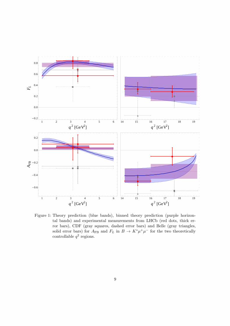
Figure 1 shows the predictions for FL and AFB with our error estimates at low andhigh q2 and compares them to the experimental data from Belle [58], CDF [77] andLHCb [6]. We do not show the data from BaBar [57], since they are given in large binsthat include q2 regions which are under poor theoretical control.
3. Model-independent constraints on Wilson coefficients
In a vast class of models beyond the SM, all NP effects in the observables listed in table 3and discussed in section 2 are described by a modification of the Wilson coefficients
C(′)7,8,9,10,S,P at a matching scale, typically of the order of heavy particles contributing to
the FCNC processes. For definiteness, we will consider in the following constraints onWilson coefficients evaluated at the scale µh = 160 GeV. The values at any other scalebelow the matching scale can be obtained straightforwardly using the renormalizationgroup [78,79], see also appendix B.
Up to subleading contributions, the coefficients C(′)8 enter the processes of interest
only via renormalization group running by the mixing of the operators O(′)7 and O(′)
8 .
Therefore, we will not consider constraints on C(′)8 in the following and keep in mind
that, in the presence of C(′)8 , the constraints on C
(′)NP7 we present can be understood as
constraints on the combination (C(′)NP7 + 0.16C
(′)NP8 ) at µh (see appendix B). Among
the observables we consider, the scalar and pseudoscalar coefficients C(′)S,P can only affect
the branching ratios of Bs → µ+µ− and Bs → τ+τ− in a significant way. Thus, we willdisregard also these coefficients and instead use the constraints on the remaining Wilsoncoefficients to give a prediction for the maximum possible sizes of BR(Bs → µ+µ−) andBR(Bs → τ+τ−) in the absence of (pseudo)scalar operators. We are thus left with the
6, potentially complex, Wilson coefficients C(′)7,9,10.
To obtain constraints on the Wilson coefficients, we construct a χ2 function, which is afunction of Wilson coefficients ~C and contains the theory predictions for the observablesOthi and the experimental central values Oexp
i as well as the corresponding uncertainties(which we assume to be Gaussian),
χ2(~C) =∑i
(Oexpi −Oth
i (~C))2
(σexpi )2 + (σth
i (~C))2. (17)
We write the theory uncertainty as a function of Wilson coefficients since, as discussedin section 2, it is a relative error for some observables and for some others, such asthe B → K∗µ+µ− angular coefficients, can even be a non-trivial function of Wilsoncoefficients.
8
à
à
òò
æ
æ
1 2 3 4 5 6-0.2
0.0
0.2
0.4
0.6
0.8
q2 @GeV2D
FL
à
à
ò
ò
æ
æ
14 15 16 17 18 19
q2 @GeV2D
ààòò
æ
æ
1 2 3 4 5 6
-0.6
-0.4
-0.2
0.0
0.2
q2 @GeV2D
AF
B
à
à
ò
ò
æ
æ
14 15 16 17 18 19
q2 @GeV2D
Figure 1: Theory prediction (blue bands), binned theory prediction (purple horizon-tal bands) and experimental measurements from LHCb (red dots, thick er-ror bars), CDF (gray squares, dashed error bars) and Belle (gray triangles,solid error bars) for AFB and FL in B → K∗µ+µ− for the two theoreticallycontrollable q2 regions.
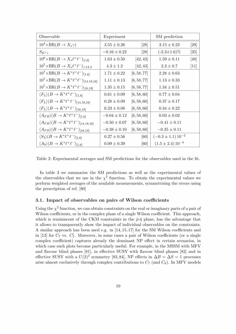
Table 2: Experimental averages and SM predictions for the observables used in the fit.
In table 3 we summarise the SM predictions as well as the experimental values ofthe observables that we use in the χ2 function. To obtain the experimental values weperform weighted averages of the available measurements, symmetrising the errors usingthe prescription of ref. [80]
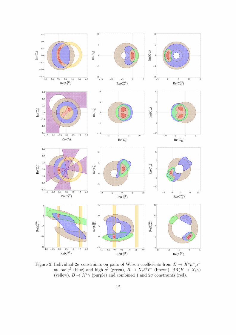
3.1. Impact of observables on pairs of Wilson coefficients
Using the χ2 function, we can obtain constraints on the real or imaginary parts of a pair ofWilson coefficients, or in the complex plane of a single Wilson coefficient. This approach,which is reminiscent of the CKM constraints in the ρ-η plane, has the advantage thatit allows to transparently show the impact of individual observables on the constraints.A similar approach has been used e.g. in [14, 15, 17] for the SM Wilson coefficients andin [12] for C7 vs. C ′7. Moreover, in some cases a pair of Wilson coefficients (or a singlecomplex coefficient) captures already the dominant NP effect in certain scenarios, inwhich case such plots become particularly useful. For example, in the MSSM with MFVand flavour blind phases [81], in effective SUSY with flavour blind phases [82] and ineffective SUSY with a U(2)3 symmetry [83, 84], NP effects in ∆B = ∆S = 1 processesarise almost exclusively through complex contributions to C7 (and C8). In MFV models
10
with dominance of Z penguins and without new sources of CP violation, only the realparts of C7 and C10 are relevant as will be discussed in section 4.
The resulting plots are shown in figure 2. In these plots, the dark and light red regionsshow the 1 and 2σ best fit regions (contours of χ2
tot−χ2tot,min = 1 or 4), while the shaded
regions in different colours show the 2σ allowed regions (contours of χ2−χ2min = 4) from
B → K∗µ+µ− at low q2 (blue), B → K∗µ+µ− at high q2 (green), B → Xs`+`− (brown),
BR(B → Xsγ) (yellow) and B → K∗γ (purple). We only show the observables that giverelevant constraints.
We make several observations.
• At the 95% C.L., all best fit regions are compatible with the SM.
• In the complex C7 plane, which is relevant e.g. for the models with flavour blindphases mentioned above, the inclusive and exclusive b → s`+`− observables – inparticular the measurement of BR(B → Xs`
+`−) at low q2 [13] and the LHCbmeasurement of AFB at low q2 – exclude a sign-flip in the low-energy Ceff
7 thatwould be allowed by BR(B → Xsγ) and that was favoured by Belle data onAFB [58]. We observe that an imaginary part of C7 as large as |Im(C7)| . 0.7 isstill allowed in this scenario.
• In the presence of C ′7, the current data on the time-dependent CP asymmetry inB → K∗γ gives already an important constraint.
• Similar to the complex C7 plane, in the Re(C7)–Re(C ′7) plane a sign-flip in Ceff7 is
excluded by the inclusive and exclusive b→ s`+`− observables. Imposing also theconstraint from SK∗γ leaves only two disjoint regions at 95% C.L.: one around theSM point and a second, less favoured one with a large Re(C ′7) ' 0.5.
• In the complex C9 and C10 planes, sign flips of the real parts are excluded butimaginary parts as large as |Im(C9)|, |Im(C10)| . 3 are still allowed.
• The slight preference towards non-SM values of the Wilson coefficients in the com-plex C ′9 and C ′10 planes results from the tension between SM prediction and ex-perimental data on BR(B → Xs`
+`−) in the high q2 region as well as the tensionbetween SM and experimental data on FL in B → K∗µ+µ− at low q2. The tensionin FL is also the reason for the slight preference for a non-SM value in the complexC ′7 plane.
• High-q2 data on B → K∗`+`− are competitive with and coplementary to the low-q2 ones. In particular, they are crucial to exclude a sign flip in Re(C10) as well assimultaneous sign flips in C10 and C ′10 or C7 and C9.
• In the Re(C9)–Re(C10) plane, a simultaneous sign flip in C9 and C10 would beallowed by high q2 data on B → K∗`+`− but is excluded by the new AFB mea-surement at low q2 from LHCb.
11
-1.0 -0.5 0.0 0.5 1.0 1.5 2.0-1.5
-1.0
-0.5
0.0
0.5
1.0
1.5
ReHC7NPL
ImHC
7L
-15 -10 -5 0 5-10
-5
0
5
10
ReHC9NPL
ImHC
9L
-5 0 5 10 15-10
-5
0
5
10
ReHC10NPL
ImHC
10L
-1.5 -1.0 -0.5 0.0 0.5 1.0 1.5-1.5
-1.0
-0.5
0.0
0.5
1.0
1.5
ReHC7' L
ImHC
7' L
-5 0 5 10-10
-5
0
5
10
ReHC9' L
ImHC
9' L
-10 -5 0 5-10
-5
0
5
10
ReHC10' L
ImHC
10'L
-1.0 -0.5 0.0 0.5 1.0 1.5 2.0-1.5
-1.0
-0.5
0.0
0.5
1.0
1.5
ReHC7NPL
ReH
C7' L
-10 -5 0 5 10
-5
0
5
10
ReHC9NPL
ReH
C9' L
-5 0 5 10 15
-10
-5
0
5
10
ReHC10NPL
ReH
C10'
L
-1.0 -0.5 0.0 0.5 1.0 1.5 2.0-15
-10
-5
0
5
ReHC7NPL
ReH
C9N
PL
-1.0 -0.5 0.0 0.5 1.0 1.5 2.0-5
0
5
10
15
ReHC7NPL
ReH
C10N
PL
-15 -10 -5 0 5-5
0
5
10
15
ReHC9NPL
ReH
C10N
PL
Figure 2: Individual 2σ constraints on pairs of Wilson coefficients from B → K∗µ+µ−
at low q2 (blue) and high q2 (green), B → Xs`+`− (brown), BR(B → Xsγ)
(yellow), B → K∗γ (purple) and combined 1 and 2σ constraints (red).
12
We stress that the above conclusions hold if one allows only the two quantities shown tobe non-zero. In many NP models, several of the Wilson coefficients will deviate from theSM, which renders some or all of these constraints ineffective. The more general casecalls for a global fit of all Wilson coefficients.
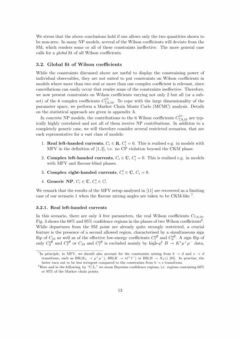
3.2. Global fit of Wilson coefficients
While the constraints discussed above are useful to display the constraining power ofindividual observables, they are not suited to put constraints on Wilson coefficients inmodels where more than two real or more than one complex coefficient is relevant, sincecancellations can easily occur that render some of the constraints ineffective. Therefore,we now present constraints on Wilson coefficients varying not only 2 but all (or a sub-
set) of the 6 complex coefficients C(′)7,9,10. To cope with the large dimensionality of the
parameter space, we perform a Markov Chain Monte Carlo (MCMC) analysis. Detailson the statistical approach are given in appendix A.
In concrete NP models, the contributions to the 6 Wilson coefficients C(′)7,9,10 are typ-
ically highly correlated and not all of them receive NP contributions. In addition to acompletely generic case, we will therefore consider several restricted scenarios, that areeach representative for a vast class of models:
1. Real left-handed currents, Ci ∈ R, C ′i = 0. This is realised e.g. in models withMFV in the definition of [1, 2], i.e. no CP violation beyond the CKM phase.
2. Complex left-handed currents, Ci ∈ C, C ′i = 0. This is realised e.g. in modelswith MFV and flavour-blind phases.
3. Complex right-handed currents, C ′i ∈ C, Ci = 0.
4. Generic NP, Ci ∈ C, C ′i ∈ C.
We remark that the results of the MFV setup analysed in [11] are recovered as a limitingcase of our scenario 1 when the flavour mixing angles are taken to be CKM-like 7.
3.2.1. Real left-handed currents
In this scenario, there are only 3 free parameters, the real Wilson coefficients C7,9,10.Fig. 3 shows the 68% and 95% confidence regions in the planes of two Wilson coefficients8.While departures from the SM point are already quite strongly restricted, a crucialfeature is the presence of a second allowed region, characterised by a simultaneous signflip of C10 as well as of the effective low-energy coefficients Ceff
7 and Ceff9 . A sign flip of
only Ceff9 and Ceff
7 or C10 and Ceff7 is excluded mainly by high-q2 B → K∗µ+µ− data,
7In principle, in MFV, we should also account for the constraints arising from b → d and s → dtransitions, such as BR(KL → µ+µ−), BR(K → π`+`−) or BR(B → Xdγ) [85]. In practise, thelatter turn out to be less stringent compared to the constraints from b→ s transitions.
8Here and in the following, by “C.L.” we mean Bayesian confidence regions, i.e. regions containing 68%or 95% of the Markov chain points.
13
0.0 0.5 1.0 1.5
-10
-5
0
C7NP
C9N
P
0.0 0.5 1.0 1.5
-2
0
2
4
6
8
10
C7NP
C10N
P
-10 -5 0
-2
0
2
4
6
8
10
C9NP
C10N
P
Figure 3: Constraints between Wilson coefficients in the scenario with real left-handedcurrents. Shown are 68% and 95% C.L. regions.
as was discussed already in [14]. Interestingly, a sign flip of only Ceff9 and C10 is now
excluded as well by the precise AFB measurement at low q2 (see section 3.1). We remarkthat an overall sign flip of all Wilson coefficients cannot be excluded by low-energy dataalone, since all observables involve squared amplitudes or interference terms, which areinvariant under such a sign flip. On the other hand, a NP model which generates effectsin C7, C9 and C10 which are each twice as large as their SM contributions seems highlyunlikely. In the region with SM-like signs, we obtain the constraints
CNP7 ∈ [−0.15, 0.03] , CNP
9 ∈ [−1.1, 1.6] , CNP10 ∈ [−1.2, 1.6] , (18)
at 95% C.L. These constraints can be translated into bounds on an effective NP scale Λthat suppresses NP contributions to the corresponding higher dimensional operators inthe effective Hamiltonian
HNPeff =
cbs7Λ2
7
O7 +cbs9Λ2
9
O9 +cbs10
Λ210
O10 + h.c. . (19)
Assuming the coefficients cbsi to be 1, and using 95% C.L. bounds on the absolute valuesof the Wilson coefficients we obtain
Λ7 > 55 TeV , Λ9 > 20 TeV , Λ10 > 21 TeV . (20)
These bounds on the effective NP scale are still weaker than the ones that can be obtainedfrom considering dimension 6 operators that contribute to Bs mixing [86].
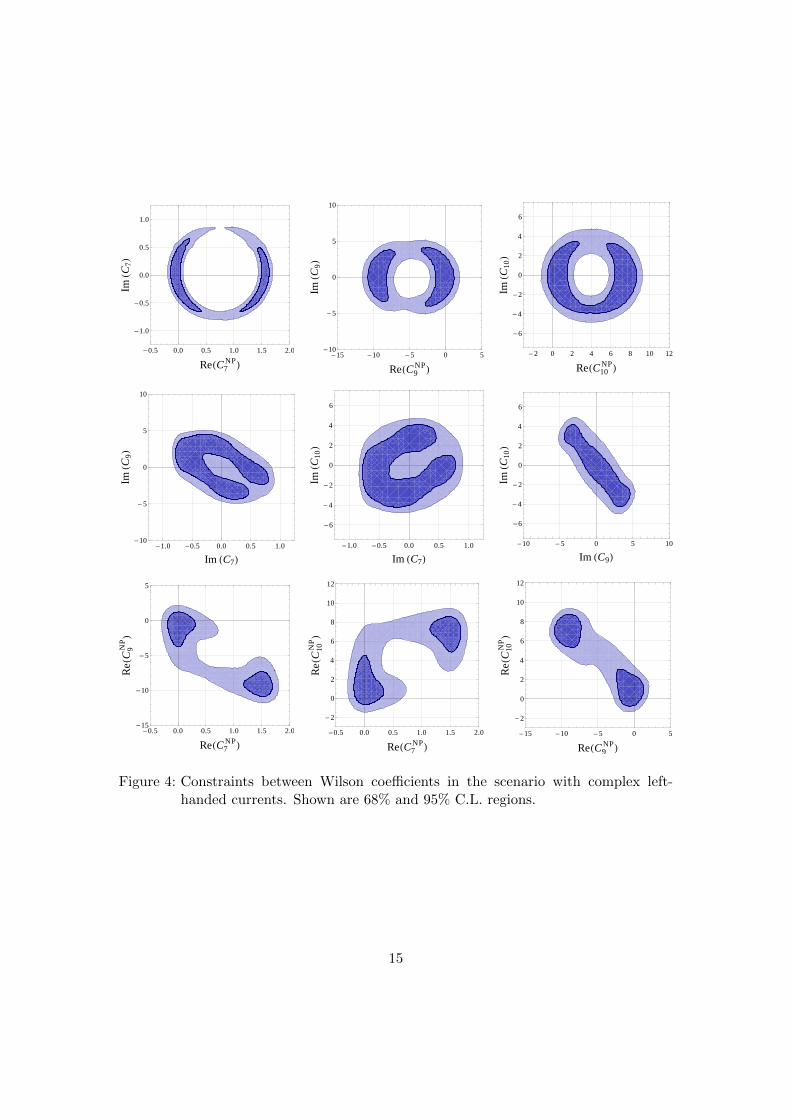
3.2.2. Complex left-handed currents
Complex contributions to the Wilson coefficients C7,9,10 with vanishing C ′i are predictede.g. in models with MFV and flavour-blind phases. Fig. 4 shows the 68% and 95%confidence regions in the planes of two Wilson coefficients, omitting plots lacking acorrelation. At 68% C.L., we observe two solutions for the real parts of the Wilson
14
-0.5 0.0 0.5 1.0 1.5 2.0
-1.0
-0.5
0.0
0.5
1.0
ReHC7NPL
ImHC 7
L
-15 -10 -5 0 5-10
-5
0
5
10
ReHC9NPL
ImHC 9
L
-2 0 2 4 6 8 10 12
-6
-4
-2
0
2
4
6
ReHC10NPL
ImHC 1
0L
-1.0 -0.5 0.0 0.5 1.0-10
-5
0
5
10
ImHC7L
ImHC 9
L
-1.0 -0.5 0.0 0.5 1.0
-6
-4
-2
0
2
4
6
ImHC7L
ImHC 1
0L
-10 -5 0 5 10
-6
-4
-2
0
2
4
6
ImHC9L
ImHC 1
0L
-0.5 0.0 0.5 1.0 1.5 2.0-15
-10
-5
0
5
ReHC7NPL
ReHC
9NP
L
-0.5 0.0 0.5 1.0 1.5 2.0
-2
0
2
4
6
8
10
12
ReHC7NPL
ReHC
10NP
L
-15 -10 -5 0 5
-2
0
2
4
6
8
10
12
ReHC9NPL
ReHC
10NP
L
Figure 4: Constraints between Wilson coefficients in the scenario with complex left-handed currents. Shown are 68% and 95% C.L. regions.
15
coefficients, corresponding to a SM-like case and a case with a simultaneous sign flipin the low-energy values of C10, Ceff
7 and Ceff9 . However, the room for NP is much
larger than in the case without non-standard CP violation since the increased number offree parameters allows for compensations among different contributions. In particular,sizable imaginary parts are allowed for all three coefficients and this implies, in turn,potentially large effects in CP violating observables, as will be quantified in sec. 3.2.6.A strong anti-correlation can be observed between the imaginary parts of C9 and C10,driven mostly by the forward-backward asymmetry in B → K∗µ+µ− at high q2.
3.2.3. Complex right-handed currents
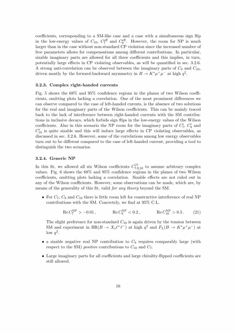
Fig. 5 shows the 68% and 95% confidence regions in the planes of two Wilson coeffi-cients, omitting plots lacking a correlation. One of the most prominent differences wecan observe compared to the case of left-handed curents, is the absence of two solutionsfor the real and imaginary parts of the Wilson coefficients. This can be mainly tracedback to the lack of interference between right-handed currents with the SM contribu-tions in inclusive decays, which forbids sign flips in the low-energy values of the Wilsoncoefficients. Also in this scenario the NP room for the imaginary parts of C ′7, C ′9 andC ′10 is quite sizable and this will induce large effects in CP violating observables, asdiscussed in sec. 3.2.6. However, some of the correlations among low energy observablesturn out to be different compared to the case of left-handed current, providing a tool todistinguish the two scenarios.
3.2.4. Generic NP
In this fit, we allowed all six Wilson coefficients C(′)7,9,10 to assume arbitrary complex
values. Fig. 6 shows the 68% and 95% confidence regions in the planes of two Wilsoncoefficients, omitting plots lacking a correlation. Sizable effects are not ruled out inany of the Wilson coefficients. However, some observations can be made, which are, bymeans of the generality of this fit, valid for any theory beyond the SM.
• For C7, C9 and C10 there is little room left for constructive interference of real NPcontributions with the SM. Concretely, we find at 95% C.L.
ReCNP7 > −0.01 , ReCNP
9 < 0.2 , ReCNP10 > 0.5 . (21)
The slight preference for non-standard C10 is again driven by the tension betweenSM and experiment in BR(B → Xs`
+`−) at high q2 and FL(B → K∗µ+µ−) atlow q2.
• a sizable negative real NP contribution to C9 requires comparably large (withrespect to the SM) positive contributions to C10 and C7.
• Large imaginary parts for all coefficients and large chirality-flipped coefficients arestill allowed.
16
-1.0 -0.5 0.0 0.5 1.0
-1.0
-0.5
0.0
0.5
1.0
ReHC7'L
ImHC 7
' L
-10 -5 0 5 10-10
-5
0
5
10
ReHC9' L
ImHC 9
' L
-6 -4 -2 0 2 4 6
-6
-4
-2
0
2
4
6
ReHC10' L
ImHC 1
0'L
-1.0 -0.5 0.0 0.5 1.0-10
-5
0
5
10
ImHC7'L
ImHC 9
' L
-1.0 -0.5 0.0 0.5 1.0
-6
-4
-2
0
2
4
6
ImHC7'L
ImHC 1
0'L
-10 -5 0 5 10
-6
-4
-2
0
2
4
6
ImHC9' L
ImHC 1
0'L
-1.0 -0.5 0.0 0.5 1.0-10
-5
0
5
10
ReHC7'L
ReHC
9' L
-1.0 -0.5 0.0 0.5 1.0
-6
-4
-2
0
2
4
6
ReHC7'L
ReHC
10'L
-10 -5 0 5 10
-6
-4
-2
0
2
4
6
ReHC9' L
ReHC
10'L
Figure 5: Constraints between Wilson coefficients in the scenario with complex right-handed currents. Shown are 68% and 95% C.L. regions.
17
-0.5 0.0 0.5 1.0 1.5 2.0
-1.0
-0.5
0.0
0.5
1.0
ReHC7NPL
ImHC 7
L
-15 -10 -5 0 5-10
-5
0
5
10
ReHC9NPL
ImHC 9
L
-2 0 2 4 6 8 10 12
-6
-4
-2
0
2
4
6
ReHC10NPL
ImHC 1
0L
-0.5 0.0 0.5 1.0 1.5 2.0
-1.0
-0.5
0.0
0.5
1.0
ReHC7NPL
ReHC
7' L
-15 -10 -5 0 5-10
-5
0
5
10
ReHC9NPL
ReHC
9' L
-2 0 2 4 6 8 10 12
-6
-4
-2
0
2
4
6
ReHC10NPL
ReHC
10'L
-0.5 0.0 0.5 1.0 1.5 2.0-15
-10
-5
0
5
ReHC7NPL
ReHC
9NP
L
-0.5 0.0 0.5 1.0 1.5 2.0
-2
0
2
4
6
8
10
12
ReHC7NPL
ReHC
10NP
L
-15 -10 -5 0 5
-2
0
2
4
6
8
10
12
ReHC9NPL
ReHC
10NP
L
Figure 6: Constraints between Wilson coefficients in the case of generic NP. Shown are68% and 95% C.L. regions.
Table 3: Predictions at 95% C.L. for the branching ratios of Bs → µ+µ− and Bs → τ+τ−
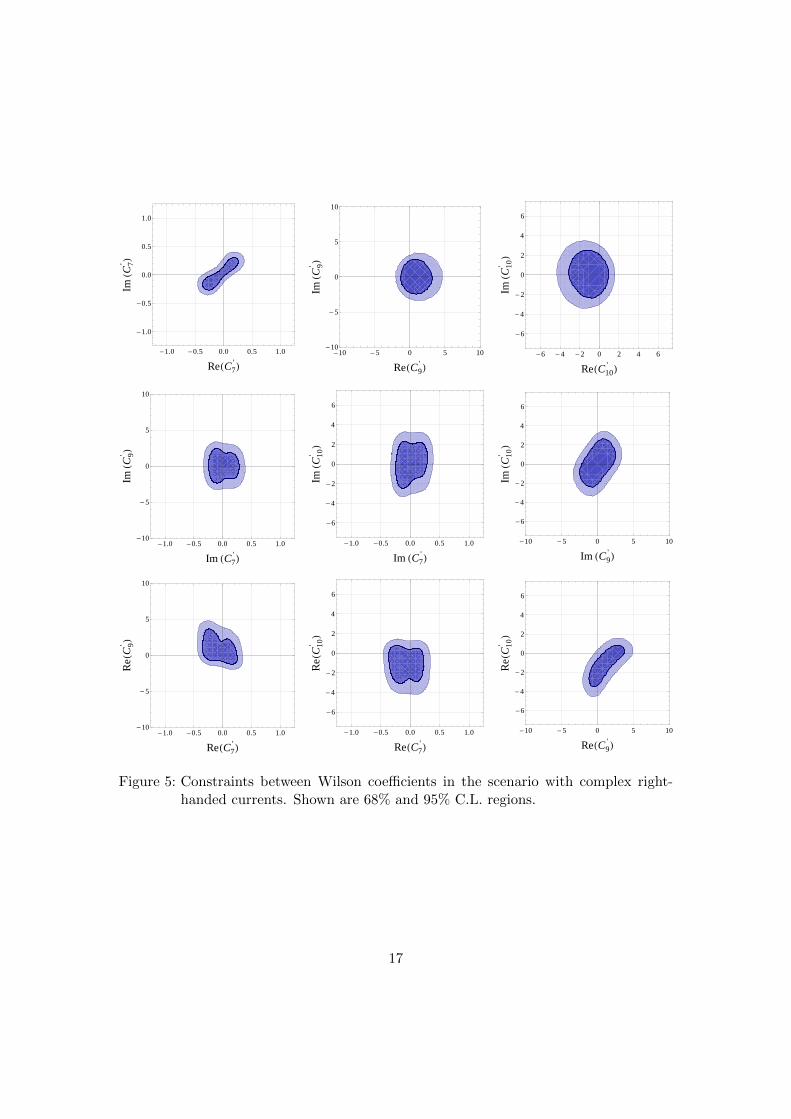
and predictions for low-q2 angular observables in B → K∗µ+µ− (neglecting tinySM effects below the percent level) in all the scenarios. The scenarios “RealLH”, “Complex LH”, “Complex RH”, “Generic NP”, “LH Z peng.”, “RH Zpeng.”, and “Generic Z p.” correspond to the scenarios discussed in sec. 3.2.1,sec. 3.2.2, sec. 3.2.3, sec. 3.2.4, sec. 4.1.1, sec. 4.1.2, and sec. 4.1.3, respectively,assuming negligible (pseudo)scalar currents. In the scenario “scalar current”only scalar currents are considered. The number quoted for Bs → τ+τ− in the“scalar current” scenario refers to the maximum value for its branching ratioin the case of dominant scalar (pseudoscalar) currents.
The last point highlights the importance of measuring observables sensitive to right-handed currents and to CP violation, such as the B → K∗µ+µ− observables A7,8,9 andS3.
3.2.5. Predictions for Bs → µ+µ− and Bs → τ+τ−
Due to its sensitivity to scalar currents, we did not include the branching ratios of
Bs → µ+µ− and Bs → τ+τ− in our fits. Instead, using the constraints on C(′)10 , we can
now give upper limits on the branching ratios in the considered scenarios assuming thescalar and pseudoscalar Wilson coefficients to be negligible. These bounds are usefulsince an observed violation of them would imply the presence of scalar currents. Thevalues we find at 95% C.L. are listed in table 3. In the scenario with right-handedcurrents as well as in the case of generic NP, a significant suppression of the branchingratios is possible. The upper bounds on BR(Bs → µ+µ−) in all cases are approximatelya factor of 2 below the current experimental bound (4) and correspond roughly to a 50%enhancement of the branching ratio with respect to the SM. Due to the new measurementof B → K∗µ+µ− angular observables, they are stronger than similar bounds presentedin the literature before [14].
19
We stress that scalar current effects in Bs → µ+µ− could still enhance the branchingratio over its current experimental bound.
Let us also mention that in the case of Bd → µ+µ−, both the effects induced by
the corresponding b → d Wilson coefficient C(′)10 and scalar currents can enhance the
branching ratio of Bd → µ+µ− over the experimental bound since the correspondingconstraints from b→ d`+`− processes are weaker. In addition, we remark that the ratioBR(Bd → µ+µ−)/BR(Bs → µ+µ−) can significantly depart from the SM as well as theMFV predictions BR(Bd → µ+µ−)/BR(Bs → µ+µ−) ≈ |Vtd/Vts|2 in both directions.
Finally, we discuss the allowed values for the branching ratio of Bs → τ+τ−. Fromthe general expressions of BR(Bs → `+`−) in presence of NP (see eq. 5) one has
BR(Bs → τ+τ−)
BR(Bs → µ+µ−)'
(1− 4m2
τ
m2Bs
)1/2m2τ
m2µ
×(1− 4m2
τ/m2Bs
)|S|2 + |P |2
|S|2 + |P |2, (22)
where S and P have been defined in eq. 6.
In the case where C(′)10 provides the dominant NP effects, one obtains
BR(Bs → τ+τ−)
BR(Bs → µ+µ−)' 212 , (23)
which implies, in particular, the SM prediction for the branching ratio of Bs → τ+τ−
BR(Bs → τ+τ−)SM = (7.7± 0.8)× 10−7 . (24)
In the case where (pseudo)scalar current effects dominate, BR(Bs → µ+µ−) can saturatethe current experimental bound while for BR(Bs → τ+τ−) we get
120 .BR(Bs → τ+τ−)
BR(Bs → µ+µ−). 212 , (25)
where the lower (upper) bound in eq. 25 correspond to the case where the scalar (pseu-doscalar) contribution dominates.
Combining eq. (3) with eq. (25), it turns out that BR(Bs → τ+τ−) . 2 × 10⁻⁶ (seealso table 3) and it has to be seen whether such values might be within the reach ofLHCb. However, we stress that this upper bound relies on the assumption that the
(pseudo)scalar Wilson coefficients C(′)S,P are linearly proportional to the lepton Yukawa
couplings, as discussed in sec. 2. If we relax this assumption, as it might be the case inmodels like R-parity violating SUSY [87] or models with enhanced couplings with thethird lepton generation (compared to the linear scaling assumed throughout this work),BR(Bs → τ+τ−) could get in principle much larger values than 10−6.
3.2.6. Predictions for B → K∗µ+µ−
Figure 7 shows the predictions for the T-odd B → K∗µ+µ− CP asymmetries A7 andA8 at low q2 for the scenarios with complex left-handed currents, complex right-handed
20
-0.4 -0.2 0.0 0.2 0.4
-0.3
-0.2
-0.1
0.0
0.1
0.2
0.3
XA7\@1,6D
XA8\ @1
,6D
-0.4 -0.2 0.0 0.2 0.4
-0.3
-0.2
-0.1
0.0
0.1
0.2
0.3
XA7\@1,6D
XA8\ @1
,6D
-0.4 -0.2 0.0 0.2 0.4
-0.3
-0.2
-0.1
0.0
0.1
0.2
0.3
XA7\@1,6D
XA8\ @1
,6D
Figure 7: Fit predictions for the low-q2 CP asymmetries 〈A7,8〉 in B → K∗µ+µ− inthe case of complex left-handed currents (left), complex right-handed currents(centre) and generic NP (right). Shown are 68% and 95% C.L. regions.
currents and for generic NP. In the absence of right-handed currents, one finds an anti-correlation between A7 and A8 which has already been found in models where only C7
contributes [55,82,84] (see also [88]), but is shown here to hold under more general con-ditions. At 68% C.L., one finds a preference for non-standard CP asymmetries drivenmostly by the tension between SM and experiment in FL(B → K∗µ+µ−) at low q2. Sim-ilarly, in the absence of complex left-handed currents, one finds an opposite correlation.In the generic case, there is no correlation at all. Interestingly, in all three scenarios,large effects in both asymmetries are still allowed, with the numerical bounds listed intable 3. Future measurements of A7 and A8 at LHCb will thus be crucial to constrainthe imaginary parts of the Wilson coefficients entering the B → K∗µ+µ− decay.
Also shown in table 3 are the predictions for the CP asymmetry A9 and the CP-averaged angular coefficient S3 at low q2, both of which are tiny in the SM but can besizable in presence of right-handed currents. Indeed, both observables can assume valuesin excess of 10% in the complex right-handed scenario and for generic NP.
We note that the CDF measurement of S3 and A9 shown in the last two rows of table 3currently puts no significant constraints on NP, yet. Future measurements at LHCb witherrors of the order of 0.1 will however put important constraints on CP-violating or CP-conserving right-handed currents.
4. Analysis of flavour-changing Z couplings
Tree level FCNC couplings of the Z boson can appear in a number of NP scenar-ios. Prominent examples are the SM with four non-sequential generations of quarksand models with an extra U(1) symmetry [89, 90]. Moreover, the contributions to thesemi-leptonic operators are dominated by Z penguins, i.e. loop-induced modified Z cou-
21
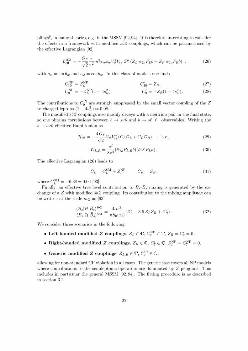
plings9, in many theories, e.g. in the MSSM [92,94]. It is therefore interesting to considerthe effects in a framework with modified sbZ couplings, which can be parametrised bythe effective Lagrangian [92]
LsbZeff = −GF√2
e
π2m2ZcwswV
∗tbVts Z
µ (ZL sγµPLb+ ZR sγµPRb) , (26)
with sw = sin θw and cw = cos θw. In this class of models one finds
CNP10 = ZNP
L , C ′10 = ZR , (27)
CNP9 = −ZNP
L (1− 4s2w) , C ′9 = −ZR(1− 4s2
w) . (28)
The contributions to C(′)9 are strongly suppressed by the small vector coupling of the Z
to charged leptons (1− 4s2w) ≈ 0.08.
The modified sbZ couplings also modify decays with a neutrino pair in the final state,so one obtains correlations between b → sνν and b → s`+`− observables. Writing theb→ sνν effective Hamiltonian as
Heff = −4GF√2VtbV
∗ts (CLOL + CROR) + h.c. , (29)
OL,R =e2
8π2(sγµPL,Rb)(νγ
µPLν) , (30)
The effective Lagrangian (26) leads to
CL = CSML + ZNP
L , CR = ZR , (31)
where CSML = −6.38± 0.06 [93].
Finally, an effective tree level contribution to Bs-Bs mixing is generated by the ex-change of a Z with modified sbZ coupling. Its contribution to the mixing amplitude canbe written at the scale mZ as [93]
〈Bs|H|Bs〉sbZ
〈Bs|H|Bs〉SM=
4αs2w
πS0(xt)(Z2
L − 3.5ZLZR + Z2R) . (32)
We consider three scenarios in the following:
• Left-handed modified Z couplings, ZL ∈ C, CNP7 ∈ C, ZR = C ′7 = 0,
• Right-handed modified Z couplings, ZR ∈ C, C ′7 ∈ C, ZNPL = CNP
allowing for non-standard CP violation in all cases. The generic case covers all NP modelswhere contributions to the semileptonic operators are dominated by Z penguins. Thisincludes in particular the general MSSM [92, 94]. The fitting procedure is as describedin section 3.2.
22
-0.5 0.0 0.5 1.0 1.5 2.0
-1.0
-0.5
0.0
0.5
1.0
ReHC7NPL
ImHC 7
L
-2 0 2 4 6 8 10 12
-6
-4
-2
0
2
4
6
ReHZLNPL
ImHZ L
L
-0.5 0.0 0.5 1.0 1.5 2.0-12
-10
-8
-6
-4
-2
0
2
ReHC7NPL
ReHZ
LNP
L
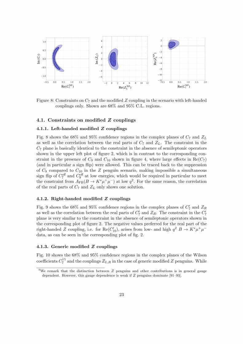
Figure 8: Constraints on C7 and the modified Z coupling in the scenario with left-handedcouplings only. Shown are 68% and 95% C.L. regions.
4.1. Constraints on modified Z couplings
4.1.1. Left-handed modified Z couplings
Fig. 8 shows the 68% and 95% confidence regions in the complex planes of C7 and ZLas well as the correlation between the real parts of C7 and ZL. The constraint in theC7 plane is basically identical to the constraint in the absence of semileptonic operatorsshown in the upper left plot of figure 2, which is in contrast to the corresponding con-straint in the presence of C9 and C10 shown in figure 4, where large effects in Re(C7)(and in particular a sign flip) were allowed. This can be traced back to the suppressionof C9 compared to C10 in the Z penguin scenario, making impossible a simultaneoussign flip of Ceff
7 and Ceff9 at low energies, which would be required in particular to meet
the constraint from AFB(B → K∗µ+µ−) at low q2. For the same reason, the correlationof the real parts of C7 and ZL only shows one solution.
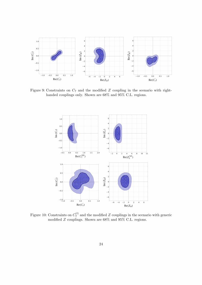
4.1.2. Right-handed modified Z couplings
Fig. 9 shows the 68% and 95% confidence regions in the complex planes of C ′7 and ZRas well as the correlation between the real parts of C ′7 and ZR. The constraint in the C ′7plane is very similar to the constraint in the absence of semileptonic operators shown inthe corresponding plot of figure 2. The negative values preferred for the real part of theright-handed Z coupling, i.e. for Re(C ′10), arises from low- and high q2 B → K∗µ+µ−
data, as can be seen in the corresponding plot of fig. 2.
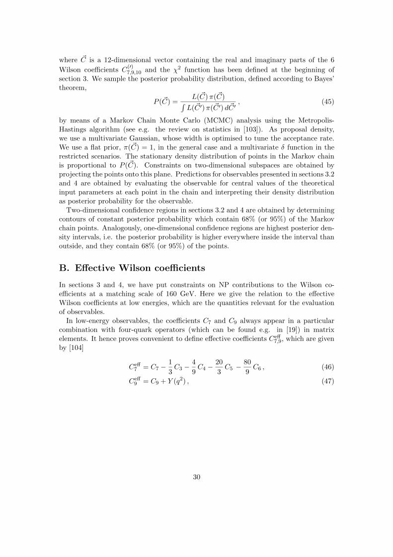
4.1.3. Generic modified Z couplings
Fig. 10 shows the 68% and 95% confidence regions in the complex planes of the Wilson
coefficients C(′)7 and the couplings ZL,R in the case of generic modified Z penguins. While
9We remark that the distinction between Z penguins and other contributions is in general gaugedependent. However, this gauge dependence is weak if Z penguins dominate [91–93].
23
-1.0 -0.5 0.0 0.5 1.0
-1.0
-0.5
0.0
0.5
1.0
ReHC7'L
ImHC 7
' L
-6 -4 -2 0 2 4 6
-6
-4
-2
0
2
4
6
ReHZRLIm
HZ RL
-1.0 -0.5 0.0 0.5 1.0
-6
-4
-2
0
2
4
6
ReHC7'L
ReHZ
RL
Figure 9: Constraints on C7 and the modified Z coupling in the scenario with right-handed couplings only. Shown are 68% and 95% C.L. regions.
-0.5 0.0 0.5 1.0 1.5 2.0
-1.0
-0.5
0.0
0.5
1.0
ReHC7NPL
ImHC 7
L
-2 0 2 4 6 8 10 12
-6
-4
-2
0
2
4
6
ReHZLNPL
ImHZ L
L
-1.0 -0.5 0.0 0.5 1.0-1.0
-0.5
0.0
0.5
1.0
ReHC7'L
ImHC 7
' L
-6 -4 -2 0 2 4 6
-6
-4
-2
0
2
4
6
ReHZRL
ImHZ R
L
Figure 10: Constraints on C(′)7 and the modified Z couplings in the scenario with generic
modified Z couplings. Shown are 68% and 95% C.L. regions.
24
-0.4 -0.2 0.0 0.2 0.4
-0.3
-0.2
-0.1
0.0
0.1
0.2
0.3
XA7\@1,6D
XA8\ @1
,6D
-0.4 -0.2 0.0 0.2 0.4
-0.3
-0.2
-0.1
0.0
0.1
0.2
0.3
XA7\@1,6D
XA8\ @1
,6D
-0.4 -0.2 0.0 0.2 0.4
-0.3
-0.2
-0.1
0.0
0.1
0.2
0.3
XA7\@1,6D
XA8\ @1
,6D
Figure 11: Fit predictions for the low-q2 CP asymmetries 〈A7,8〉 in B → K∗µ+µ− forthe scenario with left-handed (left), right-handed (centre) or generic (right)modified Z couplings. Shown are 68% and 95% C.L. regions.
the room for NP is larger than in the more constrained previous cases, also in the genericthere are no disjoint solutions for the Wilson coefficients. We are thus lead to concludeon a model-independent basis that if the NP contributions to semi-leptonic operatorsare dominated by Z penguins, the real parts of the Wilson coefficients C7,9,10 at lowenergies must have the same sign as in the SM.
4.2. Fit predictions
4.2.1. Predictions for Bs → µ+µ−, Bs → τ+τ− and B → K∗µ+µ−
Analogously to section 3.2.5, we can give fit predictions for BR(Bs → µ+µ−) andBR(Bs → τ+τ−) in the absence of scalar currents and for B → K∗µ+µ− observables inthe considered modified Z coupling scenarios based on the constraints obtained in theglobal fit. The allowed ranges are shown in table 3. In the generic case, the preferencefor smaller values of the Bs → µ+µ− and Bs → τ+τ− branching ratios is due to thenegative values preferred for Re(ZR) (cf. section 4.1.2), i.e. for Re(C ′10), which leads toa destructive interference with the SM in the decay amplitudes, see eq. (6).
Figure 11 shows the prediction for the B → K∗µ+µ− CP asymmetries A7 and A8
at low q2 in all three scenarios. The predictions are similar to the corresponding ones
obtained for generic C(′)9,10 shown in figure 7, so the comments made there apply here as
well. Also for the observables S3 and A9 we find predictions that are similar to the casesdiscussed in section 3.2.6. The results are summarised in table 3.
4.2.2. Predictions for Bs mixing
Since the real and imaginary parts of the left- and right-handed Z couplings are con-strained by b → s`+`− processes not to be significantly larger than the SM value ofthe (real) left-handed Z coupling, the Z exchange contribution to Bs mixing, which is
25
negligible in the SM, cannot lead to sizable deviations from the SM. Concretely, in theconsidered scenarios we find, at 95% C.L.,
Such NP contributions are well within the range allowed by the measurement of the Bsmixing phase at LHCb [95].
4.2.3. Predictions for b→ sνν decays
The two exclusive b → sνν decays, B → (K,K∗)νν, and the inclusive one B → Xsννgive access to four observables sensitive to NP: the three branching ratios and the K∗
longitudinal polarisation fraction FL in B → K∗νν. However, the observables are notall independent since they depend on only two real combinations of the complex Wilsoncoefficients CL and CR [93, 96,97],
ε =
√|CL|2 + |CR|2|(CL)SM|
, η =−Re (CLC
∗R)
|CL|2 + |CR|2. (36)
For the central values of the hadronic parameters, one obtains10 [93]
BR(B → K∗νν) = 6.8× 10⁻⁶ (1 + 1.31 η)ε2 , (37)
BR(B → Kνν) = 4.5× 10⁻⁶ (1− 2 η)ε2 , (38)
BR(B → Xsνν) = 2.7× 10⁻⁵ (1 + 0.09 η)ε2 , (39)
〈FL〉(B → K∗νν) = 0.54(1 + 2 η)
(1 + 1.31 η), (40)
where 〈FL〉 refers to the ratio of the branching ratio into a longitudinal K∗ over the totalbranching ratio. It can be extracted from the angular distribution of the K∗ → Kπ decayproducts.
In the scenario with left-handed modified Z couplings only, one has η = 0, FL isSM-like and all the branching ratios are merely scaled by a common factor. We obtain,at 95% C.L.,
ε2 =BR(B → K∗νν)
BR(B → K∗νν)SM=
BR(B → Kνν)
BR(B → Kνν)SM∈ [0.5, 1.3] . (41)
In the scenario with right-handed modified Z couplings and SM-like left-handed cou-plings, one finds an anticorrelation between the two experimentally most promising
10A lower central value for BR(B → Kνν) is obtained if the experimental value of BR(B → K`+`−) isused, assuming the latter decay to be SM-like [98]. Here we allow both decays to deviate from theSM prediction. We treat the B → τ(→ Kν)ν contribution [99] as a background to be subtractedfrom the experimental result.
26
0 2 4 6 8 10 12 140
2
4
6
8
10
12
106´BRHB®K ΝΝL
106 ´
BR
HB®K
* ΝΝL
Figure 12: Fit prediction for the branching ratios of B → K(∗)νν for generic modified Zcouplings. Shown are 68% and 95% C.L. regions.
modes, B → Kνν and B → K∗νν (see [88,100]). At 95% C.L., we find
BR(B → K∗νν)
BR(B → K∗νν)SM∈ [0.6, 1.0] ,
BR(B → Kνν)
BR(B → Kνν)SM∈ [1.0, 2.6] ,
〈FL〉〈FL〉SM
∈ [0.4, 1.0] ,
(42)The preference for a suppression of FL and BR(B → K∗νν) but an enhancement ofBR(B → Kνν) is again due to the negative values preferred for ZR commented on insection 4.1.2. The large enhancement possible for BR(B → Kνν) is close to the currentexperimental bound BR(B+ → K+νν) < 13× 10−6 [101].
In the case of left- and right-handed Z couplings, the correlation between the decayscarries information on the size of left- vs. right-handed currents and is thus a valuableprobe of the chirality structure of NP. In figure 12, we show the fit prediction for B →Kνν and B → K∗νν. We observe that the SM point is allowed at about 68% C.L.Also in this case, only a small enhancement or a sizable suppression is allowed for theB → K∗νν branching ratio, while an enhancement of the B → Kνν branching ratio upto a factor of 3 is possible. For FL, we find at 95% C.L.
〈FL〉〈FL〉SM
∈ [0.4, 1.1] . (43)
In all the scenarios, the full allowed range of branching ratios can be probed at thenext-generation B factories [38].
Finally, we stress that these conclusions are only valid under the assumptions thatmodified Z couplings dominate the NP contributions to b → sνν and b → s`+`− semi-leptonic operators. Much larger effects in B → K(∗)νν are possible in models where thisis not the case, e.g. models with a non-universal Z ′ coupling stronger to neutrinos thanto charged leptons [93].
27
5. Conclusions
Rare decays with a b → s transition offer excellent opportunities to probe the flavoursectors of extensions of the SM. The effects of new heavy degrees of freedom in theseprocesses can be parametrised by modifications of the Wilson coefficients of local, non-renormalizable operators, which allows to constrain such NP effects in a model-independentway. In this work, we analysed the constraints on the Wilson coefficients that follow fromthe currently available experimental data on b → s rare decays. We took into accountthe measurements from the B factories of the branching ratio of the radiative B → Xsγdecay, of the time-dependent CP asymmetry in B → K∗γ, of the branching ratio of theinclusive B → Xs`
+`− decay, Belle and CDF data on the branching ratio and angulardistribution of the exclusive B → K∗µ+µ− decay and in particular the recent LHCbresults on the branching ratio and angular distribution of B → K∗µ+µ−.
The constraints on the Wilson coefficients are obtained by using a χ2 function, whichdepends on the Wilson coefficients and contains the theory predictions for the observablesand experimental averages as well as the corresponding uncertainties.
We have analysed the following scenarios where:
1. the dominant NP effects are captured already by one complex Wilson coefficientor by a pair of real Wilson coefficients. This is a representative case of manyNP models like the MSSM with MFV and flavour blind phases [81,82], non-MFVSUSY models [83,84,102] and also models with dominance of Z penguins;
2. the NP effects are accounted for by means of the full set of the 6 complex Wilson
coefficients C(′)7,9,10.
3. the dominant NP effects in the semi-leptonic operators arise from non-standardflavour changing Z couplings.
While we refer to sections 3 and 4 for a detailed description of all our results, we wantto emphasise here the following main messages:
• At the 95% C.L., all best fit regions are compatible with the SM.
• The combination of inclusive and exclusive b → s`+`− observables exclude signflips in various low-energy WCs. That is, the SM is likely to provide the dominanteffects in low energy observables. In particular, we show that
– sign flips in C7, C9 or C10 are excluded if NP enters dominantly through Zpenguins,
– only a simultaneous sign flip of C7, C9 and C10, which cannot be excluded bylow-energy data alone, is allowed in the absence of non-standard CP violationor right-handed currents.
• The new AFB measurement at low q2 from LHCb is already quite effective inconstraining NP effects. The same is true for the time-dependent CP asymmetryin B → K∗γ.
28
• High-q2 data on B → K∗µ+µ− are competitive with and complementary to thelow-q2 ones.
Moreover, we have investigated the implications of the above constraints and the futureprospects for observables in b → s`+`− and b → sνν transitions in view of improvedmeasurements. In particular, we find that
• in the presence of non-standard CP violation, the low-q2 angular CP asymmetriesA7 and A8 in B → K∗µ+µ− can reach up to ±35% and ±20%, respectively.
• in the presence of right-handed currents, the low-q2 angular observables A9 and S3
in B → K∗µ+µ− can reach up to ±15%.
• in the absence of (pseudo)scalar currents, BR(Bs → µ+µ−) and BR(Bs → τ+τ−)can be enhanced at most by 50% over their SM values, mainly due to the newmeasurement of B → K∗µ+µ− angular observables. In contrast, if scalar currentsare at work, BR(Bs → µ+µ−) can still saturate the current experimental boundand BR(Bs → τ+τ−) can be enhanced by a factor of 3.
• if NP in b→ s`+`− and b→ sνν processes is dominated by left-handed Z penguins,an enhancement of the branching ratios of B → K(∗)νν by more than 30% isunlikely. If right-handed Z penguins are present, B → Kνν can saturate thepresent experimental bound, while B → K∗νν is unlikely to be enhanced.
The first two points highlight the importance of measuring observables in the B →K∗µ+µ− angular distribution sensitive to right-handed currents and CP violation. Suchmeasurements would be crucial to lift degeneracies in the space of Wilson coefficientswhich make it difficult at present to put strong constraints on individual coefficients ina completely generic NP model, as our analysis in sections 3.2.2 and 3.2.4 showed.
In conclusion, the present work updates and generalises previous studies providing, atthe same time, a useful tool to test the flavour structure of any theory beyond the SM.
Acknowledgements
We thank Andrzej Buras and Thorsten Feldmann for helpful discussions and ChristophBobeth and Zoltan Ligeti for useful comments. Fermilab is operated by Fermi ResearchAlliance, LLC under Contract No. De-AC02-07CH11359 with the United States Depart-ment of Energy. D.M.S. is supported by the EU ITN “Unification in the LHC Era”,contract PITN-GA-2009-237920 (UNILHC).
A. Statistical method
Here we give some details on our statistical method used to obtain the constraints on theWilson coefficients in section 3.2 and 4. We use a Bayesian approach with the likelihoodfunction
L(~C) = e−χ2( ~C)/2 , (44)
29
where ~C is a 12-dimensional vector containing the real and imaginary parts of the 6
Wilson coefficients C(′)7,9,10 and the χ2 function has been defined at the beginning of
section 3. We sample the posterior probability distribution, defined according to Bayes’theorem,
P (~C) =L(~C)π(~C)∫
L(~C ′)π(~C ′) d~C ′, (45)
by means of a Markov Chain Monte Carlo (MCMC) analysis using the Metropolis-Hastings algorithm (see e.g. the review on statistics in [103]). As proposal density,we use a multivariate Gaussian, whose width is optimised to tune the acceptance rate.We use a flat prior, π(~C) = 1, in the general case and a multivariate δ function in therestricted scenarios. The stationary density distribution of points in the Markov chainis proportional to P (~C). Constraints on two-dimensional subspaces are obtained byprojecting the points onto this plane. Predictions for observables presented in sections 3.2and 4 are obtained by evaluating the observable for central values of the theoreticalinput parameters at each point in the chain and interpreting their density distributionas posterior probability for the observable.
Two-dimensional confidence regions in sections 3.2 and 4 are obtained by determiningcontours of constant posterior probability which contain 68% (or 95%) of the Markovchain points. Analogously, one-dimensional confidence regions are highest posterior den-sity intervals, i.e. the posterior probability is higher everywhere inside the interval thanoutside, and they contain 68% (or 95%) of the points.
B. Effective Wilson coefficients
In sections 3 and 4, we have put constraints on NP contributions to the Wilson co-efficients at a matching scale of 160 GeV. Here we give the relation to the effectiveWilson coefficients at low energies, which are the quantities relevant for the evaluationof observables.
In low-energy observables, the coefficients C7 and C9 always appear in a particularcombination with four-quark operators (which can be found e.g. in [19]) in matrixelements. It hence proves convenient to define effective coefficients Ceff
7,9, which are givenby [104]
Ceff7 = C7 −
1
3C3 −
4
9C4 −
20
3C5 −
80
9C6 , (46)
Ceff9 = C9 + Y (q2) , (47)
30
with
Y (q2) = h(q2,mc)
(4
3C1 + C2 + 6C3 + 60C5
)− 1
2h(q2,mb)
(7C3 +
4
3C4 + 76C5 +
64
3C6
)− 1
2h(q2, 0)
(C3 +
4
3C4 + 16C5 +
64
3C6
)+
4
3C3 +
64
9C5 +
64
27C6 (48)
at leading order in αs and ΛQCD/mb. Beyond the leading order, there are perturbativecorrections as well as power corrections, which differ for inclusive and exclusive b →s`+`− decays. We refer the reader to Refs. [44, 45, 47–51, 69, 74] for these corrections.Ref. [70] contains the expressions for the doubly Cabibbo-suppressed contribution to(46)–(47) which is relevant for the SM prediction of the B → K∗µ+µ− CP asymmetries.
In the SM, one finds at the scale µb = 4.8 GeV, to NNLL accuracy [55],
while the primed coefficients are negligible. Beyond the SM, but assuming the four-quarkoperators to be free of NP, one has
Ceff7 (µb) = Ceff,SM
7 (µb) + CNP7 (µb) , (50)
Ceff9 (µb) = Ceff,SM
9 (µb) + CNP9 , (51)
C10 = CSM10 + CNP
10 , (52)
C ′7(µb) = C ′NP7 (µb) , (53)
C ′9,10(µb) = C ′NP9,10 . (54)
While the NP contributions to C(′)9 and C
(′)10 do not run, C
(′)7 do and they mix with C
(′)8
under renormalization. With leading order running, as is appropriate for NP contribu-tions evaluated at one loop, from a high matching scale µh = 160 GeV, one finds
C(′)NP7 (µb) = 0.623 C
(′)NP7 (µh) + 0.101 C
(′)NP8 (µh) . (55)
Since the low-energy observables are sensitive to C(′)NP7 (µb), the constraints we presented
in sections 3 and 4 on C(′)NP7 (µh) for vanishing C
(′)NP8 can be interpreted as constraints
on C(′)NP7 (µh) + 0.162 C
(′)NP8 (µh) for non-standard C
(′)8 .
References
[1] A. Buras, P. Gambino, M. Gorbahn, S. Jager, and L. Silvestrini, “Universalunitarity triangle and physics beyond the standard model,” Phys.Lett. B500(2001) 161–167, arXiv:hep-ph/0007085 [hep-ph].
[2] G. D’Ambrosio, G. Giudice, G. Isidori, and A. Strumia, “Minimal flavorviolation: An Effective field theory approach,” Nucl.Phys. B645 (2002) 155–187,arXiv:hep-ph/0207036 [hep-ph].
[3] LHCb Collaboration, “Roadmap for selected key measurements of LHCb,”arXiv:0912.4179 [hep-ex].
[4] T. Aushev, W. Bartel, A. Bondar, J. Brodzicka, T. Browder, et al., “Physics atSuper B Factory,” arXiv:1002.5012 [hep-ex].
[5] SuperB Collaboration, B. O’Leary et al., “SuperB Progress Reports – Physics,”arXiv:1008.1541 [hep-ex].
[6] LHCb Collaboration, “Angular analysis of B0 → K∗0µ+µ−,”.LHCb-CONF-2011-022.
[7] C. Bobeth, G. Hiller, and G. Piranishvili, “Angular Distributions of B → K``Decays,” JHEP 12 (2007) 040, arXiv:0709.4174 [hep-ph].
[8] C. Bobeth, G. Hiller, D. van Dyk, and C. Wacker, “The Decay B → K`+`− atLow Hadronic Recoil and Model-Independent ∆B = 1 Constraints,”arXiv:1111.2558 [hep-ph].
[9] C. Bobeth, M. Bona, A. J. Buras, T. Ewerth, M. Pierini, et al., “Upper boundson rare K and B decays from minimal flavor violation,” Nucl.Phys. B726 (2005)252–274, arXiv:hep-ph/0505110 [hep-ph].
[10] U. Haisch and A. Weiler, “Determining the Sign of the Z-Penguin Amplitude,”Phys.Rev. D76 (2007) 074027, arXiv:0706.2054 [hep-ph].
[11] T. Hurth, G. Isidori, J. F. Kamenik, and F. Mescia, “Constraints on New Physicsin MFV models: A Model-independent analysis of ∆ F = 1 processes,”Nucl.Phys. B808 (2009) 326–346, arXiv:0807.5039 [hep-ph].
[12] S. Descotes-Genon, D. Ghosh, J. Matias, and M. Ramon, “Exploring New Physicsin the C7 − C ′7 plane,” JHEP 1106 (2011) 099, arXiv:1104.3342 [hep-ph].
[13] P. Gambino, U. Haisch, and M. Misiak, “Determining the sign of the b→ sγamplitude,” Phys.Rev.Lett. 94 (2005) 061803, arXiv:hep-ph/0410155[hep-ph].
[14] C. Bobeth, G. Hiller, and D. van Dyk, “The Benefits of B → K∗`+`− Decays atLow Recoil,” JHEP 1007 (2010) 098, arXiv:1006.5013 [hep-ph].
[15] C. Bobeth, G. Hiller, and D. van Dyk, “More Benefits of Semileptonic Rare BDecays at Low Recoil: CP Violation,” JHEP 1107 (2011) 067, arXiv:1105.0376[hep-ph].
[16] G. Hiller and F. Kruger, “More model independent analysis of b→ s processes,”Phys.Rev. D69 (2004) 074020, arXiv:hep-ph/0310219 [hep-ph].
[17] C. Bobeth, G. Hiller, and G. Piranishvili, “CP Asymmetries in barB → K∗(→ Kπ)¯ and Untagged Bs, Bs → φ(→ K+K−)¯ Decays at NLO,”JHEP 0807 (2008) 106, arXiv:0805.2525 [hep-ph].
[18] C. Bobeth and U. Haisch, “New Physics in Γs12: (sb) (τ τ) Operators,”arXiv:1109.1826 [hep-ph].
[19] C. Bobeth, M. Misiak, and J. Urban, “Photonic penguins at two loops and mt
dependence of BR[B → Xs`+`−],” Nucl.Phys. B574 (2000) 291–330,
arXiv:hep-ph/9910220 [hep-ph].
[20] C. Bobeth, A. J. Buras, F. Kruger, and J. Urban, “QCD corrections toB → Xd,sνν, Bd,s → `+`−, K → πνν and KL → µ+µ− in the MSSM,”Nucl.Phys. B630 (2002) 87–131, arXiv:hep-ph/0112305 [hep-ph].
[21] J. Laiho, E. Lunghi, and R. S. Van de Water, “Lattice QCD inputs to the CKMunitarity triangle analysis,” Phys. Rev. D81 (2010) 034503, arXiv:0910.2928[hep-ph]. and online update at www.latticeaverages.org.
[22] C. McNeile, C. T. H. Davies, E. Follana, K. Hornbostel, and G. P. Lepage,“High-Precision fBs and HQET from Relativistic Lattice QCD,”arXiv:1110.4510 [hep-lat].
[23] A. J. Buras, “Relations between ∆Ms,d and Bs,d → µµ in models with minimalflavor violation,” Phys.Lett. B566 (2003) 115–119, arXiv:hep-ph/0303060[hep-ph].
[24] LHCb Collaboration, “Search for the rare decays B0(s) → µ+µ− with 300 pb−1 at
LHCb,”. LHCb-CONF-2011-037.
[25] CMS Collaboration, S. Chatrchyan et al., “Search for Bs and B to dimuondecays in pp collisions at 7 TeV,” arXiv:1107.5834 [hep-ex].
[26] LHCb and CMS Collaboration, “Search for the rare decay B0s → µ+µ− at the
LHC with the CMS and LHCb experiments,”. LHCb-CONF-2011-039,CMS-PAS-BPH-11-019.
[27] CDF Collaboration, T. Aaltonen et al., “Search for Bs → µ+µ− and Bd → µ+µ−
Decays with CDF II,” arXiv:1107.2304 [hep-ex].
[28] Heavy Flavor Averaging Group Collaboration, D. Asner et al., “Averages ofb-hadron, c-hadron, and τ -lepton Properties,” arXiv:1010.1589 [hep-ex].
[29] M. Misiak, H. Asatrian, K. Bieri, M. Czakon, A. Czarnecki, et al., “Estimate ofB(B → Xsγ) at O(α2
[30] M. Misiak and M. Steinhauser, “NNLO QCD corrections to the B → Xsγ matrixelements using interpolation in mc,” Nucl.Phys. B764 (2007) 62–82,arXiv:hep-ph/0609241 [hep-ph].
[31] E. Lunghi and J. Matias, “Huge right-handed current effects inB → K∗(Kπ)`+`− in supersymmetry,” JHEP 0704 (2007) 058,arXiv:hep-ph/0612166 [hep-ph].
[32] D. Atwood, M. Gronau, and A. Soni, “Mixing induced CP asymmetries inradiative B decays in and beyond the standard model,” Phys.Rev.Lett. 79 (1997)185–188, arXiv:hep-ph/9704272 [hep-ph].
[33] B. Grinstein, Y. Grossman, Z. Ligeti, and D. Pirjol, “The photon polarization inB → Xγ in the standard model,” Phys. Rev. D71 (2005) 011504,arXiv:hep-ph/0412019.
[34] P. Ball and R. Zwicky, “Time-dependent CP Asymmetry in B → K∗γ as a(Quasi) Null Test of the Standard Model,” Phys.Lett. B642 (2006) 478–486,arXiv:hep-ph/0609037 [hep-ph].
[35] P. Ball, G. W. Jones, and R. Zwicky, “B → V γ beyond QCD factorisation,”Phys.Rev. D75 (2007) 054004, arXiv:hep-ph/0612081 [hep-ph].
[36] Belle Collaboration, Y. Ushiroda et al., “Time-Dependent CP Asymmetries inB0 → K0
Sπ0γ transitions,” Phys.Rev. D74 (2006) 111104,
arXiv:hep-ex/0608017 [hep-ex].
[37] BaBar Collaboration, B. Aubert et al., “Measurement of Time-Dependent CPAsymmetry in B0 → K0
Sπ0γ Decays,” Phys.Rev. D78 (2008) 071102,
arXiv:0807.3103 [hep-ex].
[38] B. Meadows, M. Blanke, A. Stocchi, A. Drutskoy, A. Cervelli, et al., “The impactof SuperB on flavour physics,” arXiv:1109.5028 [hep-ex].
[39] J. M. Soares, “CP violation in radiative b decays,” Nucl.Phys. B367 (1991)575–590.
[40] A. L. Kagan and M. Neubert, “Direct CP violation in B → Xsγ decays as asignature of new physics,” Phys.Rev. D58 (1998) 094012,arXiv:hep-ph/9803368 [hep-ph].
[41] M. Benzke, S. J. Lee, M. Neubert, and G. Paz, “Long-Distance Dominance of theCP Asymmetry in B → Xs,d + γ Decays,” Phys.Rev.Lett. 106 (2011) 141801,arXiv:1012.3167 [hep-ph].
[42] BaBar Collaboration, B. Aubert et al., “Measurement of the B → Xs`+`−
branching fraction with a sum over exclusive modes,” Phys.Rev.Lett. 93 (2004)081802, arXiv:hep-ex/0404006 [hep-ex].
[44] H. Asatrian, H. Asatrian, C. Greub, and M. Walker, “Two loop virtualcorrections to B → Xs`
+`− in the standard model,” Phys.Lett. B507 (2001)162–172, arXiv:hep-ph/0103087 [hep-ph].
[45] H. Asatryan, H. Asatrian, C. Greub, and M. Walker, “Calculation of two loopvirtual corrections to b→ s`+`− in the standard model,” Phys.Rev. D65 (2002)074004, arXiv:hep-ph/0109140 [hep-ph].
[46] C. Bobeth, P. Gambino, M. Gorbahn, and U. Haisch, “Complete NNLO QCDanalysis of B → Xs`
+`− and higher order electroweak effects,” JHEP 0404(2004) 071, arXiv:hep-ph/0312090 [hep-ph].
[47] A. Ghinculov, T. Hurth, G. Isidori, and Y. Yao, “The Rare decay B → Xs`+`−
to NNLL precision for arbitrary dilepton invariant mass,” Nucl.Phys. B685(2004) 351–392, arXiv:hep-ph/0312128 [hep-ph].
[48] T. Huber, E. Lunghi, M. Misiak, and D. Wyler, “Electromagnetic logarithms inB → Xs`
[51] C. Greub, V. Pilipp, and C. Schupbach, “Analytic calculation of two-loop QCDcorrections to b→ s`+`− in the high q2 region,” JHEP 0812 (2008) 040,arXiv:0810.4077 [hep-ph].
[52] K. S. Lee, Z. Ligeti, I. W. Stewart, and F. J. Tackmann, “Universality and mX
cut effects in B → Xs`+`−,” Phys.Rev. D74 (2006) 011501,
arXiv:hep-ph/0512191 [hep-ph].
[53] G. Bell, M. Beneke, T. Huber, and X.-Q. Li, “Heavy-to-light currents at NNLOin SCET and semi-inclusive B → Xs`
[54] T. E. Browder, T. Gershon, D. Pirjol, A. Soni, and J. Zupan, “New Physics at aSuper Flavor Factory,” Rev.Mod.Phys. 81 (2009) 1887–1941, arXiv:0802.3201[hep-ph].
[55] W. Altmannshofer, P. Ball, A. Bharucha, A. J. Buras, D. M. Straub, andM. Wick, “Symmetries and Asymmetries of B → K∗µ+µ− Decays in theStandard Model and Beyond,” JHEP 0901 (2009) 019, arXiv:0811.1214[hep-ph].
[56] U. Egede, T. Hurth, J. Matias, M. Ramon, and W. Reece, “New observables inthe decay mode Bd → K∗0l+l−,” JHEP 0811 (2008) 032, arXiv:0807.2589[hep-ph].
[57] BaBar Collaboration, B. Aubert et al., “Angular Distributions in the DecaysB → K∗`+`−,” Phys.Rev. D79 (2009) 031102, arXiv:0804.4412 [hep-ex].
[58] Belle Collaboration, J.-T. Wei et al., “Measurement of the DifferentialBranching Fraction and Forward-Backword Asymmetry for B → K(∗)`+`−,”Phys.Rev.Lett. 103 (2009) 171801, arXiv:0904.0770 [hep-ex].
[59] CDF Collaboration, T. Aaltonen et al., “Measurement of the Forward-BackwardAsymmetry in the B → K(∗)µ+µ− Decay and First Observation of theB0s → φµ+µ− Decay,” Phys.Rev.Lett. 106 (2011) 161801, arXiv:1101.1028
[hep-ex].
[60] CDF Collaboration, T. Aaltonen et al., “Measurements of the AngularDistributions in the Decays B → K(∗)µ+µ− at CDF,” arXiv:1108.0695
[hep-ex].
[61] F. Kruger and J. Matias, “Probing new physics via the transverse amplitudes ofB0 → K∗0(→ K−pi+)l+l− at large recoil,” Phys.Rev. D71 (2005) 094009,arXiv:hep-ph/0502060 [hep-ph].
[62] A. K. Alok, A. Dighe, D. Ghosh, D. London, J. Matias, et al., “New-physicscontributions to the forward-backward asymmetry in B → K∗µ+µ−,” JHEP1002 (2010) 053, arXiv:0912.1382 [hep-ph].
[63] E. Lunghi and A. Soni, “An improved observable for the forward-backwardasymmetry in B → K∗l+l− and Bs → φl+l−,” JHEP 1011 (2010) 121,arXiv:1007.4015 [hep-ph].
[64] A. K. Alok, A. Datta, A. Dighe, M. Duraisamy, D. Ghosh, et al., “New Physicsin b→ sµ+µ−: CP-Conserving Observables,” arXiv:1008.2367 [hep-ph].
[65] A. K. Alok, A. Datta, A. Dighe, M. Duraisamy, D. Ghosh, et al., “New Physicsin b→ sµ+µ−: CP-Violating Observables,” arXiv:1103.5344 [hep-ph].
[66] U. Egede, T. Hurth, J. Matias, M. Ramon, and W. Reece, “New physics reach ofthe decay mode B → K∗0`+`−,” JHEP 1010 (2010) 056, arXiv:1005.0571[hep-ph].
[67] A. Bharucha and W. Reece, “Constraining new physics with B → K∗µ+µ− in theearly LHC era,” Eur.Phys.J. C69 (2010) 623–640, arXiv:1002.4310 [hep-ph].
[68] A. Khodjamirian, T. Mannel, A. Pivovarov, and Y.-M. Wang, “Charm-loop effectin B → K(∗)`+`− and B → K∗γ,” JHEP 1009 (2010) 089, arXiv:1006.4945[hep-ph].
[69] M. Beneke, T. Feldmann, and D. Seidel, “Systematic approach to exclusiveB → V `+`−, V γ decays,” Nucl.Phys. B612 (2001) 25–58,arXiv:hep-ph/0106067 [hep-ph].
[70] M. Beneke, T. Feldmann, and D. Seidel, “Exclusive radiative and electroweakb→ d and b→ s penguin decays at NLO,” Eur.Phys.J. C41 (2005) 173–188,arXiv:hep-ph/0412400 [hep-ph].
[71] P. Ball and R. Zwicky, “Bd,s → ρ, ω,K∗, φ decay form-factors from light-conesum rules revisited,” Phys.Rev. D71 (2005) 014029, arXiv:hep-ph/0412079[hep-ph].
[72] B. Grinstein and D. Pirjol, “Exclusive rare B → K∗`+`− decays at low recoil:Controlling the long-distance effects,” Phys.Rev. D70 (2004) 114005,arXiv:hep-ph/0404250 [hep-ph].
[73] M. Beylich, G. Buchalla, and T. Feldmann, “Theory of B → K(∗)l+l− decays athigh q2: OPE and quark-hadron duality,” Eur.Phys.J. C71 (2011) 1635,arXiv:1101.5118 [hep-ph].
[74] D. Seidel, “Analytic two loop virtual corrections to b→ dl+l−,” Phys.Rev. D70(2004) 094038, arXiv:hep-ph/0403185 [hep-ph].
[75] CKMfitter Collaboration, J. Charles et al., “CP violation and the CKMmatrix: Assessing the impact of the asymmetric B factories,” Eur.Phys.J. C41(2005) 1–131, arXiv:hep-ph/0406184 [hep-ph]. updated results and plotsavailable at: http://ckmfitter.in2p3.fr.
[76] A. Bharucha, T. Feldmann, and M. Wick, “Theoretical and PhenomenologicalConstraints on Form Factors for Radiative and Semi-Leptonic B-Meson Decays,”JHEP 1009 (2010) 090, arXiv:1004.3249 [hep-ph].
[77] CDF Collaboration, T. Aaltonen et al., “Observation of the BaryonicFlavor-Changing Neutral Current Decay Λ0
b → Λµ+µ−,” arXiv:1107.3753
[hep-ex].
[78] K. G. Chetyrkin, M. Misiak, and M. Munz, “Weak radiative B meson decaybeyond leading logarithms,” Phys.Lett. B400 (1997) 206–219,arXiv:hep-ph/9612313 [hep-ph].
[79] M. Gorbahn, U. Haisch, and M. Misiak, “Three-loop mixing of dipole operators,”Phys.Rev.Lett. 95 (2005) 102004, arXiv:hep-ph/0504194 [hep-ph].
[80] G. D’Agostini, “Asymmetric uncertainties: Sources, treatment and potentialdangers,” arXiv:physics/0403086 [physics].
[81] W. Altmannshofer, A. Buras, and P. Paradisi, “Low Energy Probes of CPViolation in a Flavor Blind MSSM,” Phys.Lett. B669 (2008) 239–245,arXiv:0808.0707 [hep-ph].
[82] R. Barbieri, P. Lodone, and D. M. Straub, “CP Violation in Supersymmetry withEffective Minimal Flavour Violation,” JHEP 1105 (2011) 049, arXiv:1102.0726[hep-ph].
[83] R. Barbieri, G. Isidori, J. Jones-Perez, P. Lodone, and D. M. Straub, “U(2) andMinimal Flavour Violation in Supersymmetry,” Eur.Phys.J. C71 (2011) 1725,arXiv:1105.2296 [hep-ph].
[84] R. Barbieri, P. Campli, G. Isidori, F. Sala, and D. M. Straub, “B-decayCP-asymmetries in SUSY with a U(2)3 flavour symmetry,” arXiv:1108.5125
[hep-ph].
[85] A. Crivellin and L. Mercolli, “B → Xdγ and constraints on new physics,”arXiv:1106.5499 [hep-ph].
[86] G. Isidori, Y. Nir, and G. Perez, “Flavor Physics Constraints for Physics Beyondthe Standard Model,” Ann.Rev.Nucl.Part.Sci. 60 (2010) 355, arXiv:1002.0900[hep-ph].
[87] R. Barbier, C. Berat, M. Besancon, M. Chemtob, A. Deandrea, et al., “R-parityviolating supersymmetry,” Phys.Rept. 420 (2005) 1–202,arXiv:hep-ph/0406039 [hep-ph].
[88] D. M. Straub, “New physics correlations in rare decays,” arXiv:1012.3893
[hep-ph].
[89] P. Langacker and M. Plumacher, “Flavor changing effects in theories with aheavy Z ′ boson with family nonuniversal couplings,” Phys.Rev. D62 (2000)013006, arXiv:hep-ph/0001204 [hep-ph].
[90] P. Langacker, “The Physics of Heavy Z-prime Gauge Bosons,” Rev. Mod. Phys.81 (2009) 1199–1228, arXiv:0801.1345 [hep-ph].
[91] A. J. Buras and L. Silvestrini, “Upper bounds on K → πνν and KL → π0e+e−
from ε′/ε and KL → µ+µ−,” Nucl.Phys. B546 (1999) 299–314,arXiv:hep-ph/9811471 [hep-ph].
[92] G. Buchalla, G. Hiller, and G. Isidori, “Phenomenology of nonstandard Zcouplings in exclusive semileptonic b→ s transitions,” Phys.Rev. D63 (2000)014015, arXiv:hep-ph/0006136 [hep-ph].
[93] W. Altmannshofer, A. J. Buras, D. M. Straub, and M. Wick, “New strategies forNew Physics search in B → K∗νν, B → Kνν and B → Xsνν decays,” JHEP0904 (2009) 022, arXiv:0902.0160 [hep-ph].
[95] LHCb Collaboration, “Combination of φs measurements from B0s → J/ψφ and
B0s → J/ψf0(980),”. LHCb-CONF-2011-056.
[96] Y. Grossman, Z. Ligeti, and E. Nardi, “New limit on inclusive B → Xsνν decayand constraints on new physics,” Nucl.Phys. B465 (1996) 369–398,arXiv:hep-ph/9510378 [hep-ph].
[97] D. Melikhov, N. Nikitin, and S. Simula, “Right-handed currents in rare exclusiveB → (K,K∗)νν decays,” Phys.Lett. B428 (1998) 171–178,arXiv:hep-ph/9803269 [hep-ph].
[98] M. Bartsch, M. Beylich, G. Buchalla, and D.-N. Gao, “Precision Flavour Physicswith B → Kνν and B → K`+`−,” JHEP 0911 (2009) 011, arXiv:0909.1512[hep-ph].
[99] J. F. Kamenik and C. Smith, “Tree-level contributions to the rare decaysB+ → π+νν, B+ → K+νν, and B+ → K∗+νν in the Standard Model,”Phys.Lett. B680 (2009) 471–475, arXiv:0908.1174 [hep-ph].
[100] A. J. Buras, K. Gemmler, and G. Isidori, “Quark flavour mixing withright-handed currents: an effective theory approach,” Nucl.Phys. B843 (2011)107–142, arXiv:1007.1993 [hep-ph].
[101] BaBar Collaboration, P. del Amo Sanchez et al., “Search for the Rare DecayB → Kνν,” Phys.Rev. D82 (2010) 112002, arXiv:1009.1529 [hep-ex].
[102] W. Altmannshofer, A. J. Buras, S. Gori, P. Paradisi, and D. M. Straub,“Anatomy and Phenomenology of FCNC and CPV Effects in SUSY Theories,”Nucl. Phys. B830 (2010) 17–94, arXiv:0909.1333 [hep-ph].
[103] Particle Data Group Collaboration, K. Nakamura et al., “Review of particlephysics,” J.Phys.G G37 (2010) 075021.
[104] A. Buras, M. Misiak, M. Munz, and S. Pokorski, “Theoretical uncertainties andphenomenological aspects of B → Xγ decay,” Nucl.Phys. B424 (1994) 374–398,arXiv:hep-ph/9311345 [hep-ph].