A ckno - i11 · and Alexander „Sascha“ Wolff, as well as Dominik Schultes from the neighboring...

Engineering Planar-Separatorand Shortest-Path Algorithmszur Erlangung des akademis hen Grades einesDoktors der Naturwissens haftender Fakultät für Informatikder Universität Frideri iana zu Karlsruhe (TH)genehmigteDissertationvonMartin Holzeraus Rottweil

Tag der mündli hen Prüfung: 13.06.2008Erste Guta hterin: Prof. Dr. Dorothea WagnerZweiter Guta hter: Prof. Dr. Matthias Müller-Hannemann

A knowledgmentsAs soon as some piece of work of a major scale has been accomplished, all the preceding

labor, setbacks, and occasional frustration are forgotten, and new-found serenity sets in.

That point in time is also an excellent occasion to thank all those people who accompanied

that project and—in one way or the other—guided the person conducting it. Thus, it is

now my pleasure to greatfully acknowledge all the support I received while working for

my PhD.

First of all, I’d like to thank my advisor Dorothea Wagner for encouraging me to join her

group: from among plenty of things, it was the trusting and respectful working environ-

ment that I enjoyed in particular. It was also Dorothea who in the first place respected

my burning desire for spending some time abroad, and strongly supported my stay at

Virginia Tech. Besides various occasions to attend great conferences and summer schools,

which didn’t exactly always take place in Germany or even Europe, I also got the chance to

participate in the university-teaching certificate program.

Next, I’d like to thank my colleagues, Reinhard Bauer, office mate Michael Baur, Marc

Benkert, Daniel Delling, Marco Gaertler, Robert Görke (who, ungrudgingly, also took the

toil of proof-reading this tome), Bastian Katz, Marcus Krug, Steffen Mecke, Sascha Mei-

nert, Martin Nöllenburg, Ignaz Rutter, Thomas Schank, Étienne Schramm, Silke Wagner,

and Alexander „Sascha“ Wolff, as well as Dominik Schultes from the neighboring group,

for the fruitful and harmonious collaboration during the entire time. In my first year, it was

Frank Schulz and Thomas Willhalm in particular who took me under their wings. My

gratitude extends to all co-authors not named in person.

A big thank-you goes to our secretaries, Lilian Beckert, Elke Sauer, and Nihal Yagi-

zefe, as well as to our systems administrator, Bernd Giesinger, whose great work in the

background became the most evident whenever they were not there. This whole project

would also not have been possible without the loyal assistance of our students, Imen Borgi,

Jürgen Graf, Sebastian Knopp, Valentin Mihaylov, Jens Müller, Kirill Müller, Andrea

Schumm, and Tirdad Rahmani, who greatly helped with the implementation and evalua-

tion, but also came up with inspiring new ideas.

During my four-month stay in Blacksburg, I enjoyed the wonderful hospitality by the

group of Chris Barrett, and manyfold advice especially from Madhav Marathe (thanks

also to my close friends, Scott Russell and Haris Volos, for greatly enriching my stay).

I furthermore received generous financial support through a fellowship granted by the

German Academic Exchange Service (DAAD).

Special thanks go to Matthias Müller-Hannemann from the University of Halle for

readily accepting the task of reviewing my dissertation, as well as the rest of the commit-

tee, examiners Ralf Reussner and Peter Sanders and chairman Roland Vollmar.

Finally, support for my endeavors was by no means restricted to my working environment,

but crucially granted through personal relationships. Heartfelt thanks to my family—my

devoted parents, my wonderful sisters, Petra and Katrin, and my dear partner, Tobias—for

all their love and assistance: einfach vielen Dank für alles! Though not by name, I won’t forget

to mention all those close friends of mine, with whom I share a great deal of memories.

Last but not least, I’d like to thank all those unnamed people who by their proactive help,

still inspiration, or simple presence enriched my life.

Martin Holzer Karlsruhe, August 13, 2008

Contents1 Zusammenfassung (German Summary) 1

2 Introduction 5

2.1 Overview . . . . . . . . . . . . . . . . . . . . . . . . . . . . . . . . . . . . . . . . 6

2.2 Fundamentals . . . . . . . . . . . . . . . . . . . . . . . . . . . . . . . . . . . . . 9

2.2.1 Graphs . . . . . . . . . . . . . . . . . . . . . . . . . . . . . . . . . . . . . 9

2.2.2 Shortest-Path Search . . . . . . . . . . . . . . . . . . . . . . . . . . . . . 10

3 Planar Separation 13

3.1 Motivation . . . . . . . . . . . . . . . . . . . . . . . . . . . . . . . . . . . . . . . 14

3.1.1 Related Work . . . . . . . . . . . . . . . . . . . . . . . . . . . . . . . . . 15

3.2 Algorithms . . . . . . . . . . . . . . . . . . . . . . . . . . . . . . . . . . . . . . . 17

3.2.1 Algorithm Description . . . . . . . . . . . . . . . . . . . . . . . . . . . . 17

3.2.2 Optimization . . . . . . . . . . . . . . . . . . . . . . . . . . . . . . . . . 19

3.3 Heuristics . . . . . . . . . . . . . . . . . . . . . . . . . . . . . . . . . . . . . . . 21

3.3.1 BFS Variants . . . . . . . . . . . . . . . . . . . . . . . . . . . . . . . . . . 21

3.3.2 Tree Height Control . . . . . . . . . . . . . . . . . . . . . . . . . . . . . 22

3.3.3 Triangulating BFS . . . . . . . . . . . . . . . . . . . . . . . . . . . . . . . 23

3.3.4 Star Trees . . . . . . . . . . . . . . . . . . . . . . . . . . . . . . . . . . . 24

3.3.5 Postprocessing . . . . . . . . . . . . . . . . . . . . . . . . . . . . . . . . 25

3.4 Graphs . . . . . . . . . . . . . . . . . . . . . . . . . . . . . . . . . . . . . . . . . 26

3.5 Experiments . . . . . . . . . . . . . . . . . . . . . . . . . . . . . . . . . . . . . . 29

3.5.1 Algorithmic Comparison . . . . . . . . . . . . . . . . . . . . . . . . . . 29

3.5.2 Graph Series . . . . . . . . . . . . . . . . . . . . . . . . . . . . . . . . . 35

3.5.3 Heuristics . . . . . . . . . . . . . . . . . . . . . . . . . . . . . . . . . . . 40

3.5.4 Postprocessing . . . . . . . . . . . . . . . . . . . . . . . . . . . . . . . . 41

3.5.5 Recommendation . . . . . . . . . . . . . . . . . . . . . . . . . . . . . . . 41

3.6 Discussion . . . . . . . . . . . . . . . . . . . . . . . . . . . . . . . . . . . . . . . 42

Contents4 Multi-Level Technique 43

4.1 Motivation . . . . . . . . . . . . . . . . . . . . . . . . . . . . . . . . . . . . . . . 44

4.1.1 Related Work . . . . . . . . . . . . . . . . . . . . . . . . . . . . . . . . . 45

4.2 Overlay Graphs . . . . . . . . . . . . . . . . . . . . . . . . . . . . . . . . . . . . 48

4.2.1 Shortest-Path Overlay Graph . . . . . . . . . . . . . . . . . . . . . . . . 48

4.2.2 Basic Multi-Level Graph . . . . . . . . . . . . . . . . . . . . . . . . . . . 50

4.2.3 Extended Multi-Level Graph . . . . . . . . . . . . . . . . . . . . . . . . 50

4.3 Shortest-Path Search . . . . . . . . . . . . . . . . . . . . . . . . . . . . . . . . . 52

4.4 Regular Multi-Level Graphs . . . . . . . . . . . . . . . . . . . . . . . . . . . . . 55

4.4.1 Theoretical Analysis . . . . . . . . . . . . . . . . . . . . . . . . . . . . . 55

4.4.2 Component-Induced Random Graphs . . . . . . . . . . . . . . . . . . . 56

4.5 Experimental Analysis . . . . . . . . . . . . . . . . . . . . . . . . . . . . . . . . 58

4.5.1 Selecting Vertices . . . . . . . . . . . . . . . . . . . . . . . . . . . . . . . 58

4.5.2 Graph Classes . . . . . . . . . . . . . . . . . . . . . . . . . . . . . . . . . 61

4.5.3 Shortest-Path Overlay Graphs . . . . . . . . . . . . . . . . . . . . . . . 62

4.5.4 Special Selection Criteria . . . . . . . . . . . . . . . . . . . . . . . . . . 63

4.5.5 Multi-Level Approach . . . . . . . . . . . . . . . . . . . . . . . . . . . . 65

4.6 Discussion . . . . . . . . . . . . . . . . . . . . . . . . . . . . . . . . . . . . . . . 71

5 Multimodal Routing 73

5.1 Overview . . . . . . . . . . . . . . . . . . . . . . . . . . . . . . . . . . . . . . . . 74

5.1.1 Motivation . . . . . . . . . . . . . . . . . . . . . . . . . . . . . . . . . . . 74

5.1.2 Related Work . . . . . . . . . . . . . . . . . . . . . . . . . . . . . . . . . 76

5.2 Foundation . . . . . . . . . . . . . . . . . . . . . . . . . . . . . . . . . . . . . . . 78

5.2.1 Problem Statement . . . . . . . . . . . . . . . . . . . . . . . . . . . . . . 78

5.2.2 Product Network . . . . . . . . . . . . . . . . . . . . . . . . . . . . . . . 79

5.2.3 Applications . . . . . . . . . . . . . . . . . . . . . . . . . . . . . . . . . . 79

5.3 Algorithms . . . . . . . . . . . . . . . . . . . . . . . . . . . . . . . . . . . . . . . 81

5.3.1 Speed-up Techniques . . . . . . . . . . . . . . . . . . . . . . . . . . . . . 81

5.3.2 Implementation . . . . . . . . . . . . . . . . . . . . . . . . . . . . . . . . 84

5.4 Experimental Study . . . . . . . . . . . . . . . . . . . . . . . . . . . . . . . . . . 86

5.4.1 Setup . . . . . . . . . . . . . . . . . . . . . . . . . . . . . . . . . . . . . . 87

5.4.2 Multimodal Routing . . . . . . . . . . . . . . . . . . . . . . . . . . . . . 88

5.4.3 k-Similar Paths . . . . . . . . . . . . . . . . . . . . . . . . . . . . . . . . 96

5.5 Adaptations . . . . . . . . . . . . . . . . . . . . . . . . . . . . . . . . . . . . . . 97

5.6 Discussion . . . . . . . . . . . . . . . . . . . . . . . . . . . . . . . . . . . . . . . 100

List of Figures 109

ContentsList of Tables 111

Résumé 113

Chapter 1ZusammenfassungUm meine Arbeit über die Entwicklung von Algorithmen zur planaren Separierung und Kürzeste-

Wege-Berechnung einer internationalen Leserschaft zugänglich zu machen, habe ich die vor-

liegende Dissertation in englischer Sprache verfasst. Der nachfolgende knappe Abriss soll

daher lediglich einen groben Überblick über die behandelten Themen sowie die wichtigsten

im Rahmen der Arbeit erzielten Ergebnisse vermitteln.Überbli kAuf dem Gebiet der angewandten Algorithmik begegnet einem immer öfter der Begriff des

Algorithm Engineering: hierunter wird meist ein zirkulärer Prozess verstanden, bei dem für

eine konkrete Problemstellung neue algorithmische Herangehensweisen entwickelt bzw.

bestehende Verfahren schrittweise verfeinert werden; diese werden anschließend auf einer

Menge typischer Eingaben mit dem Ziel weiterer Effizienzsteigerung empirisch evaluiert.

Da solche Algorithmen oft sehr vielfältige Anwendungen haben, mehrere Stellschrauben

bedient werden und überdies die Eingaben erheblich voneinander abweichen können, ist

eine grundlegende Voraussetzung für weitere Optimierung das Wissen um den Einfluss

von Parameterwahl und Eingabecharakteristik auf das Rechenergebnis. Kern dieser Arbeit

ist daher eine systematische Studie mehrerer Algorithmen mit dreierlei Fragestellung:

1. Auf welche Weise können unterschiedliche Eingaben hinsichtlich ihrer ‚Komplexität‘

und ihres Laufzeitverhaltens eingeordnet werden?

2. Welche Empfehlungen für eine Parameterwahl können, abhängig vom Typus der Ein-

gabe, gegeben werden?

3. Welches sind im Hinblick auf Laufzeitverhalten kritische Stellen im Algorithmus, und

wie können diese mit Hilfe neuentwickelter Heuristiken oder durch geschickte Kom-

bination bereits bestehender Ansätze effizienter implementiert werden?

1 Zusammenfassung (German Summary) 2Ausgangspunkt meiner Betrachtungen sind drei Graphenalgorithmen, die alle ein diver-

ses Anwendungsspektrum aufweisen und als Basisroutinen in einer Vielzahl komplexerer

Algorithmen zum Einsatz kommen:

• Bei der planaren Separierung soll in einem planaren, d. h. kreuzungsfrei in die Ebene

einbettbaren Graphen eine ‚kleine‘ Mengen von Knoten so bestimmt werden, dass

nach deren Wegnahme der Graph in (mindestens) zwei Zusammenhangskomponen-

ten ‚ähnlicher Größe‘ zerfällt. Solche Zerlegungen werden z. B. bei Divide-and-Conquer-

Verfahren verwendet: hierbei wird eine gegebene Probleminstanz so lange rekursiv in

zwei (oder mehr) Teilinstanzen aufgeteilt, bis diese elementar lösbar sind; die Teillö-

sungen werden anschließend wieder zu einer Gesamtlösung zusammengesetzt. Ein

allgemein bekannter Linearzeitalgorithmus für dieses Problem konnte zwar nach und

nach theoretisch verbessert werden, allerdings existierte unserer Kenntnis nach bis-

lang keine umfassendere Studie zu dessen Praxisverhalten.

• Bei der Kürzeste-Wege-Berechnung wird in einem gewichteten Graphen eine kürzes-

te (schnellste, günstigste etc.) Route zwischen zwei ausgewählten Knoten gesucht.

Dieses Problem ist Kern zahlreicher Anwendungen und stellt eine Grundherausfor-

derung insbesondere im Zusammenhang mit Verkehrsinformationssystemen, Rou-

tenplanungssoftware und Navigationsgeräten dar. Gegenstand unserer Forschung ist

eine Multilevel-Technik, die ursprünglich für die Berechnung von Zugverbindungen

entwickelt wurde. In dieser Arbeit werden nun mehrere Verbesserungen dieses An-

satzes vorgestellt und auf einer Vielzahl von Graphen ausgiebig getestet.

• In Fortführung des vorgenannten Problems sollen bei der multimodalen Wegesuche kür-

zeste Routen bestimmt werden, die gewissen Einschränkungen unterworfen sind: da-

zu werden die Kanten des Graphen mit zusätzlichen Beschriftungen versehen, wo-

bei die Beschriftung eines kürzesten Pfades einer vorgegebenen Bedingung genügen

muss. Diese Formulierung erlaubt eine einheitliche Behandlung sehr unterschiedli-

cher Probleme im Bereich der Netzplanung, wie z. B. bei Reiseauskunftssystemen, die

verschiedene Straßenkategorien oder Transportmittel berücksichtigen. In der vorlie-

genden Arbeit wird nun die konkrete Implementierung eines Lösungsalgorithmus

sowie Anpassungen einiger unimodaler Beschleunigungstechniken vorgestellt und in

verschiedenen Anwendungsszenarien auf zahlreichen Kombinationen von Netzwer-

ken und Pfadbedingungen evaluiert.ErgebnisseDer Hauptbeitrag meiner Arbeit ist in den folgenden Punkten begründet:

1 Zusammenfassung (German Summary) 3• Im Zusammenhang mit Separationsalgorithmen konnte gezeigt werden, dass die

Mehrzahl in der Praxis vorkommender Instanzen weit bessere Zerlegungen zulas-

sen, als durch die theoretischen Schranken vorgegeben. Weiterhin konnten mehrere

Subroutinen identifiziert werden, die sich signifikant auf die Separationsqualität aus-

wirken. Mit Hilfe einfacher Heuristiken konnte so sowohl die Separatorgröße als auch

die Komponentenverteilung beträchtlich optimiert werden.

Eine weitere Anwendung unserer Implementation besteht in der Berechnung ei-

ner Menge ausgewählter Knoten eines Graphen, die wiederum als Eingabe für den

Multilevel-Algorithmus gebraucht wird: zwar werden in unserer Arbeit etliche wei-

tere solcher Auswahlkriterien betrachtet; es stellt sich jedoch heraus, dass dieses Se-

paratorkriterium – zusammen mit einem weiteren – für alle Testinstanzen am besten

abschneidet.

• In einer theoretischen Analyse konnte gezeigt werden, dass der in der Vorberech-

nungsphase des Multilevel-Algorithmus beinhaltete Dekompositionsschritt einen ent-

scheidenden Einfluss auf das Laufzeitverhalten hat; dies wurde außerdem empi-

risch bestätigt. Weiterhin konnten hinsichtlich einer geeigneten Wahl der entsprechen-

den Eingabeparameter ein paar einfache Faustregeln angegeben werden, wodurch es

möglich ist, bei der Kürzeste-Wege-Berechnung auf unterschiedlichsten Graphklassen

brauchbare Beschleunigungen zu erzielen. Einige Zusammenhänge, die im Rahmen

der Studie aufgezeigt wurden, haben sich auch als recht bedeutsam für die Entwick-

lung zweier sehr ähnlicher Ansätze erwiesen.

• Ausgehend von einem Algorithmus zur Kürzeste-Wege-Berechnung mit Pfadbe-

schränkung durch reguläre Sprachen, bei dem die vorgegebene Restriktion durch einen

nichtdeterministischen Automaten repräsentiert wird, stellen wir eine praktische Im-

plementation sowie Anpassungen einiger Standardbeschleunigungstechniken vor. Im

experimentellen Teil der Studie ergaben sich einige überraschende Erkenntnisse im

Vergleich zur unimodalen Anwendung: so zeigten sich bei der multimodalen Suche

zum Teil erhebliche Abweichungen in der Robustheit dieser Techniken gegenüber

Eingabegraph und Eigenschaften der Restriktion.

Chapter 2Introdu tionIn this preliminary chapter, we expose our motivation for this work in algorithm engineer-

ing, giving a terse overview of the topics investigated and outlining the main contribution

arising from our study. The second part of this chapter provides some foundation from

the area of graph algorithmics and fixes some basic notation and conventions shared by

the subsequent parts of this work; more specific definitions can be found in the respective

chapters.

2.1 Introdu tion · Overview 62.1 OverviewIn the area of applied algorithmics, the term of algorithm engineering is being used with in-

creasing frequency: by this name we denote the circular process of designing, implement-

ing, testing, analyzing, and refining computational proceedings to tackle a given problem

for a set of possible instances more efficiently. Since such algorithms are often of fairly

general applicability, typically come with various parameters to be adjusted, and inputs to

them may vary considerably, one important premise to increasing their performance is to

have a basic understanding of the impact of both parameter settings and input characteris-

tics on the algorithmic outcome.

Our goal is to use insights gained from a systematic algorithmic study with respect to

three main purposes: classifying different kinds of input in terms of their typical runtime

complexity and behavior; drawing concrete recommendations for choosing the parameters

involved, depending on the input type; and identifying crucial parts of the algorithm for

which to devise new—or combine existing—approaches and heuristics in order to improve

algorithmic performance. This dissertation deals with algorithm engineering in the context

of graph algorithmics. We consider three problems, each of them with a broad range of

applications and being used as a core routine in a number of more complex algorithms:

• Planar separation: given a planar graph, i. e., a graph for which there exists a drawing

in the plane without any edge crossings, the objective is to find a ‘small’ number

of vertices such that upon removal of these, the graph falls apart into (at least) two

connected components of ‘similar size’. Such separations are used, e. g., with divide-

and-conquer algorithms, which solve a certain problem by recursively splitting a given

instance into two (or more) subinstances, until these can be tackled at an elementary

level; the partial solutions are then assembled to obtain one for the initial instance.

One well-known algorithm for this problem, running in time linear in the size of the

input graph, has been refined a couple of times with respect to theoretic bounds, but,

to our knowledge, no extensive study on its actual performance had been conducted.

• Single-pair shortest-path routing, where for a given graph with edge weights and two

dedicated vertices a shortest path between these vertices is requested. Solving this

problem constitutes a general and common requirement in a variety of applications:

many commercial systems basically have to tackle this very task, ranging from public-

transportation travel information software and on-line routing platforms to car navi-

gation devices. We rely on a multi-level technique initially devised to speed up shortest-

path computation on railway networks, describe several steps of improvement, and in

a comprising experimental study explore these new algorithmic variants applied also

to different graphs.

2.1 Introdu tion · Overview 7• Multimodal shortest-path routing: similarly to the aforementioned problem, the goal

is to find a shortest path between some distinct vertices, where each of the graph’s

edges (or vertices) is additionally assigned some label and the labels on a shortest path

must fulfill a given condition. This formulation covers a diverse range of applications,

many of them arising in network planning, such as travel information while distin-

guishing between different street categories or means of transportations. In our work,

we propose a concrete implementation of an algorithm solving this problem along

with several speed-up techniques known from the unimodal scenario, and experi-

mentally evaluate our programs with various combinations of applications, networks,

and restrictions.

From this brief description it may already become clear that the latter of our two rout-

ing problems constitutes a generalization of the former, which is why similar ideas and

concepts can be adopted for both. Another linkage between these topics concerns the ap-

plication of our planar-separator algorithms to compute so-called selected vertices needed for

the multi-level technique: although several other ways of doing so have been considered as

well, using planar separators is one of two methods performing best for all instances tested.

Shortest-path computation is one of the fields in computer science that has for the last

couple of years been evolving at a bewildering speed, which is equally true for the size of

many kinds of real-world graphs (especially in the realm of traffic-planning). It therefore

hardly surprises to notice that the multi-level technique as developed some few years ago

cannot quite live up to today’s standards any more. However, the systematic investigation

conducted, involving a large number of parameter settings and graphs, has delivered some

valuable insights into the behavior of this technique in realistic scenarios. Such findings

strongly helped spark development of two of the presently quickest shortest-path algo-

rithms for road networks, the high-performance multi-level technique and transit node routing,

both closely related to our approach.

At a fairly abstract level, we see the main contribution of our work in the following

achievements:

• For the planar-separator algorithms, we have shown that the majority of instances

occurring in practice allow for separations that are far from reaching the theoretic

bounds given on separator size. We have also identified some subroutines in the clas-

sic planar-separator algorithms that crucially influence separator quality. Through

combination of a few simple heuristics implementing these subprocedures, both av-

erage separator size and component balance could be improved considerably.

• Through theoretic deliberations as well as the already-mentioned empiric study we

have pointed out how performance of the multi-level routing technique depends on

the decomposition of the input graph, which forms a part of the preprocessing step

2.1 Introdu tion · Overview 8involved. This approach permits to tune quite a number of input parameters, so

we have developed some simple rules of thumb to obtain a reasonable set of initial

settings.

• For multimodal shortest-path routing, we have described a practical way of imple-

menting an algorithm using a nondeterministic automaton to model path restrictions

as well as employing several standard speed-up approaches. Revisiting these tech-

niques in the multimodal scenario has revealed some substantial deviation in robust-

ness from unimodal performance: experiments have confirmed some fundamental

dependencies of algorithmic performance on both network and automaton proper-

ties.Stru turing. The remainder of this work is canonically structured according to the three

general topics mentioned above. Each chapter contains an individual assessment of previ-

ous work in relation to ours; open questions as well as suggestions for future work on each

subject are gathered in the discussing sections.

2.2 Introdu tion · Fundamentals 92.2 FundamentalsAs exposed in the previous section, all problems considered in this work stem from the

realm of graph algorithmics, so it is important to fix some elementary graph-related terms

and notation recurrently used in the following. Two of our topics deal with shortest-path

computation: we therefore provide a brief introduction to this field, giving the algorithm

most commonly used in practice, Dijkstra’s algorithm, which is also employed in our work.

For further foundation in graph theory we recommend [AMO93].2.2.1 GraphsWe subdivide our definitions into a general part and one regarding planar separation.General De�nitions. A directed graph G = (V, E) consists of a finite set V of vertices—or

nodes1—linked by edges (v1, v2) ∈ E ⊆ V ×V, where v1 and v2 are also referred to by tail

and head vertex, respectively; in contrast, the edge set E ⊆ (V2) of an undirected graph consists

of unordered pairs {v1, v2} of vertices.2 The number of vertices is traditionally denoted by

n, the number of edges by m. Two vertices are called adjacent if they are linked by an edge,

and an edge e is incident with a vertex v (and vice versa) if v is contained in the ordered

pair or unordered set constituting e, respectively.

The edges of a graph can be assigned weights (which are mostly real- or even integer-

numbered), also named (edge) lengths or costs.3 Graphs from the area of shortest-path

computation, in particular such representing road networks, usually come with (two-

dimensional) coordinates associated with their vertices—in fact, vertex coordinates are also

often delivered by graph generators.

A (v1-vk-)path p in a graph G is defined to be a sequence of vertices 〈v1, v2, . . . , vk〉 (for

some k ≥ 1) such that for each i ∈ {1, 2, . . . , k− 1} there exists an edge {vi, vi+1} or (vi, vi+1)

in G, respectively. A path with identical end-vertices v1 and vk is called a cycle, and a simple

cycle if furthermore its vertices are pairwise distinct. If G is weighted, the length of p is

defined as the sum of lengths of the edges on p. Finally, a graph G is called connected if

there exists a path in G between every pair of vertices.

1In the literature, these terms are used synonymously and with similar frequen y; for purely histori al reasons,we employ vertex mainly with shortest-path problems and node with planar separators.2In this work, we onsider with shortest-path problems mainly the more general ase of dire ted graphs, whileplanar-separator algorithms are usually formulated for undire ted graphs. Note, however, that the shortest-pathalgorithms presented for dire ted graphs an be applied to undire ted ones by assuming for an undire ted edgearbitrary `orientation' (where typi ally the orientation is �xed on e the edge has been pro essed in one dire tion), orby repla ing ea h undire ted edge with two dire ted ones, pointing in opposite dire tions. On the other hand, ourplanar-separator algorithms an be applied to dire ted graphs by merging two edges in opposite dire tions betweenthe same nodes to one undire ted one and ignoring orientation otherwise.3An unweighted graph an be emulated through a weighted one by assuming uniform weight of 1 for ea h edge.

2.2 Introdu tion · Fundamentals 10De�nitions Regarding Planar Separation. A geometric embedding of a graph G in the plane

is a mapping of G’s nodes and edges to two-dimensional space (e. g., node coordinates

yield a canonical embedding placing the nodes at the very coordinates and representing

the edges by continuous curves). In contrast, a combinatorial embedding does not ‘prescribe

any concrete drawing’, but settles for indicating the (circular) order of edges incident with

each node. A graph is called planar if it has a geometric embedding in the plane such that

no two edges cross.

Given a geometric embedding of a planar graph, each area ‘minimally enclosed’ by a

number of edges (and their incident nodes) is called a face, where the unbounded area en-

compassing the graph is also named outer face. A planar graph whose every face is bounded

by exactly three edges is called triangulated; similarly, a triangulation of any planar graph

is obtained by adding to the graph nonintersecting edges so long until it is triangulated.

A tree is a connected graph not containing any cycles, and a spanning tree of an n-

node graph contains exactly n nodes (and n− 1 edges). All nodes of a (connected) graph

G = (V, E), along with a subset of its edges, can be enumerated through a breadth-first search

(BFS), starting at some vertex r ∈ V and enumerating its incident edges, while iteratively

proceeding with their incident head vertices in a FIFO order. The (uniformly weighted) tree

consisting of all nodes and the enumerated edges is accordingly called BFS tree with root r,

and the length of a shortest path from node v ∈ V to root r is referred to as v’s BFS level.

Last, given a weighted graph G = (V, E), the eccentricity of a node v ∈ V is defined to

be the maximal distance from v to any other node in G. Minimal eccentricity over all nodes

in the graph is also denoted by radius, maximal eccentricity by diameter.2.2.2 Shortest-Path Sear hStandard variants of the shortest-path problem are defined as follows. Given a weighted

graph G = (V, E) and a start—or source—vertex s ∈ V, the single-source shortest-path prob-

lem consists in finding for each vertex v ∈ V a path p from s to v such that the length of p

is smallest amongst all s-v-paths in G.4 The single-pair shortest-path problem is a restriction

hereof in that only a shortest s-t-path is searched, for a given target vertex t. One further

variant, however, not detailed here, is the all-pairs shortest-path problem, where for each

pair of vertices a shortest path is requested.

The single-source/single-pair problems are typically distinguished with respect to the

type of edge lengths accepted: for the case of arbitrary (integer or real-valued) lengths,

a classic, O(nm)-time solving algorithm for graphs with n vertices and m edges is given

in [Bel58], often referred to as the Belmann-Ford algorithm or label-correcting algorithm. For

the special case of nonnegative edge lengths, more efficient algorithms have been found.

4Note that in many settings, one impli itly settles for omputing only shortest distan es.

2.2 Introdu tion · Fundamentals 11Input: Directed graph G = (V, E) with edge length function l : E → R

+ \ {0}, startvertex s.

Output: Shortest distances from s to all vertices in G.Data Structures: Priority queue Q, associative container D of distance labels.for vertex v ∈ G \ {s} do1

set D[v] ← ∞2

set D[s] ← 03

push s→ Q with key D[s]4

while Q not empty do5

pop v← Q with smallest key6

for outgoing edge e = (v, v′) ∈ E do7

if D[v] + l(e) < D[v′] then8

if D[v′] = ∞ then9

set D[v′]← D[v] + l(e)10

push v′ → Q with key D[v′]11

else12

set D[v′]← D[v] + l(e)13

decrease key of v′14 Algorithm 2.1: Dijkstra's algorithm.Dijkstra's Algorithm. One of the earliest algorithms for single-source shortest-path compu-

tation on graphs with nonnegative edge lengths was given by Dijkstra [Dij59]. The basic

idea behind Dijkstra’s algorithm is to run a BFS variant on the given graph, while organiz-

ing the processed vertices in a priority queue according to an estimation of their distances

to the start vertex, based on the information gathered up to that point in time. Figure 2.1

gives a pseudocode listing.

It can be shown that this algorithm always terminates, and the values of D are then the

desired shortest distances. A straightforward implementation runs in time O(n2), whereas

using a Fibonacci heap for implementation of the priority queue, as suggested in [FT87],

takes only O(m + n log n) time. The single-pair variant can be solved by including between

lines 6 and 7 the condition if v 6= t (for some given target vertex t); note that this does not

decrease asymptotic running time, as all vertices of the graph might have to be considered

anyway, however, better performance in practice is possible. For a vertex v, the actual s-

v-path, instead of just the shortest distance, can be obtained through a simple procedure

visiting the path edges backwards from v to s, guided by the D values (which now give

accurate shortest distances).

Chapter 3Planar SeparationA common strategy to tackle algorithmic problems on graphs is to divide the input graph

into several pieces in order to distribute the computation of a solution according to some

parallelization scheme or divide-and-conquer approach. Following such a proceeding, typ-

ical side constraints may consist in some tradeoff between balancing the load attributed

to each processor or each step of recursion, respectively, and keeping small the overhead

of assembling the partial results to an overall solution. Moreover, there are a number of

problems for which simpler or more efficient algorithms have been found for the case of

planar instead of general graphs.

One way to divide up a graph with respect to the above requirements is to determine

a small subset of its nodes whose removal splits the graph into two components of similar

size. For planar graphs, this can be achieved through the well-known Planar-Separator

Theorem by Lipton and Tarjan, which guarantees separators of size√

8n and components

of size less than 2n/3, where n denotes the number of nodes in the graph. Although

this work was published some 30 years ago, and has since been refined several times at a

conceptual level, no broader investigation of practical performance has been conducted.

By this study, we remedy that deficiency: we evaluate two classic planar-separator al-

gorithms (the one derived from the Planar-Separator Theorem as well as one further de-

velopment due to Djidjev) applied to a large variety of graphs, where our goal is not only

to satisfy the given bounds on separator and component sizes, but to heuristically opti-

mize these values. The original algorithmic descriptions are given at a fairly abstract level,

such that several degrees of freedom regarding a concrete implementation arise, for which

we provide a number of specific alternatives. Experiments show that the choice of these

parameters influences separation quality considerably.

3.1 Planar Separation · Motivation 143.1 MotivationNode separators are often employed for divide-and-conquer approaches, where an instance of

a graph problem is solved by recursively splitting it up into subinstances, until these can

be tackled smoothly; then the partial solutions found are combined to a complete one. In

particular, for a number of problems, such as finding maximum matchings, more efficient

algorithms could be devised for instances restricted to planar graphs, through the use of

node separators. Because the depth of recursion is minimal when the subinstances are of

similar size, and the overhead of assembling the partial solutions typically increases with

the number of separator nodes, in practice we are interested in algorithms separating a

graph into balanced subgraphs through a small number of nodes.

An interesting analogy to the divide-and-conquer paradigm from the realm of molec-

ular biology is protein folding, which is the process of polypeptides (i. e., linear chains of

amino acids) transforming themselves into 3D structures. In a recent paper [OWCD07], it is

suggested that this folding takes place as a zipping-and-assembly process, where zipping de-

notes growing of local substructures within the polypeptide, and the assembly part refers

to interaction between these substructures. This physical model has in turn led to more

efficient algorithms for computing the stereometric structure of proteins by determining

certain folding points, which are used to split up the given instance.

In [LT79], Lipton and Tarjan introduce the Planar-Separator Theorem: for every planar

graph with n ≥ 5 nodes there is a subset of its nodes—called (node) separator—of size at

most√

8n ≈ 2.83√

n such that the remaining nodes can be grouped into two sets—also

referred to by components—each of which contains at most 2n/3 nodes, and no edge passes

between these components. The proof of this theorem is constructive in the sense that an

algorithm can be derived from it fairly easily, which can be implemented in linear time.

Djidjev [Dji82] improves the upper bound on separator size to√

6n ≈ 2.45√

n, paralleled

by a refinement of Lipton and Tarjan’s algorithm; he also proves a lower bound of 1.56√

n,

which is still the best known. These classic algorithms both proceed in two stages, where

they share the second. The first, or simple, stage of each algorithm tries to determine a

separator that meets the given bounds, induced by one or two levels of nodes of a breadth-

first search tree; only upon failure, the second, or complex, stage kicks in, which always

succeeds in finding an appropriate separator, based on a simple, or fundamental, cycle.

Although these algorithms have been known for quite some time, we are not aware of

any systematic study exploring them experimentally. In this work, we therefore investigate

their behavior with respect to various graphs, both generated and from real world (exhibit-

ing considerable differences in properties like density, minimum separator size, diameter

etc.). However, not only do we settle for satisfying the upper bounds on separator size

and component balance, but strive to improve on these values (we also employ a tradeoff

measure named ratio, as suggested in [LR99]).

3.1 Planar Separation · Motivation 15Besides exploring the above algorithms, we propose the use of fundamental-cycle separa-

tion (FCS) in its own right, i. e., mere application of the second stage, omitting the first. This

strategy guarantees a separator bound of roughly twice the diameter of the input graph,

which often beats the O(√

n) bounds for graphs with small diameter. Further motivation

for this engineering work comes from the fact that many subroutines shared by the classic

algorithms are not fixed with respect to every detail: for the breadth-first search (BFS) per-

formed at the simple stage, neither the root node nor the order in which to visit incident

edges and adjacent nodes are specified; also, the complex stage requires a triangulation of

the graph and selection of a non-tree edge, but no further assumptions are made.

Preliminary results showed the importance of an appropriate choice of the BFS root

node: since testing all nodes in the graph would incur quadratic running time, we rather

propose different heuristic methods to draw a selection of root nodes to be considered.

For execution of a BFS, given a fixed root, we also evaluate several schemes of visiting

neighboring edges and nodes; variation of the search order does not affect distribution

of the nodes to BFS levels, however, ‘balance’ of the tree edges is influenced, which may

have an impact on the performance of both heuristics and the complex stage. Finally,

we introduce a breadth-first search variant called triangulating BFS, which determines a

triangulation while simultaneously recomputing the BFS tree.3.1.1 Related WorkWe divide our synopsis of preceding work on planar-graph separation into three parts:

the first discusses further developments of Lipton and Tarjan’s results; the second deals

with generalized and restricted variants of the base problem; finally, the third part briefly

mentions some applications of planar-separator algorithms.Classi Separation. For the case of 2/3-separations (i. e., each component may comprise at

most 2/3 of the graph’s nodes), the genuine Planar-Separator Theorem [LT79] gives an

upper bound on separator size of√

8n ≈ 2.83√

n. This result is improved by Djidjev [Dji82]

to√

6n ≈ 2.45√

n, which is achieved by a more sophisticated proceeding at the first stage of

the algorithm. Since then, this bound has been lowered several times, to√

4.5n ≈ 2.12√

n by

Alon, Seymour, and Thomas [AST94] and to the currently best value of 1.97√

n by Djidjev

and Venkatesan [DV97]. The latter work also gives a lower bound of 1.56√

n on the size of

planar node separators, due to an analysis of specifically-constructed globe graphs.

Spielman and Teng [ST96] prove an algorithm for separation of a planar graph into two

components of at most 3n/4 nodes each, through a set of no more than√

3.5n ≈ 1.84√

n

nodes. Only for the sake of completeness we want to mention that there are results on

1/2-separations reported in the literature, where the leading factors of the O(√

n)-bounds

are, naturally, much higher.

3.1 Planar Separation · Motivation 16Generalizations and Variants. In [ADGM06], Aleksandrov et al. consider a generalization of

the classic problem, called t-separators: given a planar graph with cost and weight for each

node, total cost C, and a balance factor t ∈ (0, 1), the objective is to find a node separator

with total cost not exceeding C such that the weight of each remaining component is at

most t times the total weight of the graph. Such separations typically yield more than two

components; setting t = 2/3 and using unit weights and costs covers the genuine variant

due to Lipton and Tarjan. The paper includes an experimental study with a few synthetic

and real-world graphs; in contrast, our work focuses on analyzing degrees of freedom

inherent to the two classic algorithms and exploiting concrete ways of implementing them

to improve separation quality in practice.

Concerning special graph classes, [Mil84] shows that for each 2-connected planar graph

with maximum face size d there exists a simple-cycle 2/3-separation of size O(2√

2dn).Appli ations. As explained above, one of the most prominent problems for which planar-

separator algorithms are employed is recursive decomposition of a planar graph according

to a divide-and-conquer paradigm, where a straightforward implementation would yield

a running time of O(n log n). In [Goo95], some refined strategies are presented to obtain

a linear-time decomposition algorithm. Another application of recursive decomposition

is shortest-path search on planar graphs [Fre87], where separators consisting of O(n/√

r)

nodes and splitting the graph into Θ(n/r) components of size O(r) are used. Finally,

[AFN03] describes parameterized algorithms for different graph problems which rely on

planar separators.

3.2 Planar Separation · Algorithms 173.2 AlgorithmsIn this section, we describe in more detail the algorithms tested empirically, where we start

by revisiting the Planar-Separator Theorem and the corresponding algorithm by Lipton

and Tarjan [LT79]. We further motivate the use of the second stage of the algorithm as a

stand-alone procedure, called fundamental-cycle separation. For our experiments, we envision

three optimization criteria, which partly lead to some algorithmic modifications; in particular,

implementing the optimized version of the complex stage requires a little deliberation.3.2.1 Algorithm Des riptionWe state the Planar-Separator Theorem in a slightly modified form so that it covers the

results of both Lipton/Tarjan’s and Djidjev’s works (for the sake of simplicity, we consider

unweighted graphs here, although the algorithms—and actually our implementations—

work for the weighted case as well).

Theorem 3.2.1 (Planar-Separator Theorem [generalized version]). Given a planar graph G =

(V, E) with n ≥ 5 nodes. The nodes in V can be partitioned into three sets A, B, and S such that

no edge joins a node in A with a node in B, neither A nor B consists of more than 2n/3 nodes, and

S contains at most β√

n nodes (for some constant β).

Using this notation, the separator bound due to Lipton/Tarjan is given by β =√

8,

while Djidjev’s bound takes β =√

6. However, our implementation of Lipton/Tarjan’s

algorithm was done according to a textbook version with β = 4 [Meh84, Koz92].Lipton and Tarjan's Algorithm (LT)The algorithm arising from the proof of the Planar-Separator Theorem proceeds in two

stages, which we call simple and complex; the simple stage can be subdivided into two parts,

phases 1 and 2. For the sake of consistency, we refer to the complex stage also by phase 3.

It is noteworthy that all steps of the algorithm can be implemented in linear time. For an

illustration of the different phases, cf. Figure 3.1.Simple Stage. Phase 1 starts by computing a breadth-first search (BFS) tree, thus grouping

the nodes into levels, where the BFS root be located at level 0. Then the middle level

is defined to be the level with the smallest index µ such that all levels with indexes at

most µ encompass at least half of the graph’s nodes. If this middle level contains fewer

nodes than given by the separator bound, the algorithm returns that level (note that due to

construction, the balance requirement is always met); otherwise, the algorithm continues

with phase 2.

3.2 Planar Separation · Algorithms 18

Figure 3.1: The three phases of Lipton and Tarjan's algorithm (simpli�ed illustration; non-tree edges aregenerally omitted). From left to right: phase 1 (simple stage; one BFS level, µ), phase 2 (simple stage; twoBFS levels, m and M), and phase 3 ( omplex stage; two BFS levels plus fundamental y le). Separatornodes are marked in bla k; red and blue oloring re�e ts omponent membership of the remaining nodes.The dashed gray lines ut o� the nodes temporarily merged and removed during phase 3, respe tively; thenon-tree edge indu ing the fundamental y le (green path) is drawn dashed-green.In phase 2, starting at the middle level, the levels above and below (i. e., with smaller

and with greater indexes) are scanned until in each direction a level of at most 2(√

n− D)

nodes is found, where D is the respective distance to the middle level. These two levels,

with indexes denoted by m and M, yield a separation of the remaining nodes into three

parts. If the biggest of these parts and the other two combined each meet the balance

bound, the two levels are returned as a separator. Otherwise, the algorithm enters the

complex stage.Complex Stage. Temporarily all levels with indexes greater or equal to M are removed from

the graph and levels 0 to m are merged to one node; the remaining graph is triangulated.

Every non-tree edge e induces a path in the BFS tree from each of e’s end-nodes to their

‘nearest’ common ancestor; these paths together with e form a fundamental cycle, dividing

the remaining nodes into an inner and an outer part. From all non-tree edges, the algorithm

picks one arbitrarily. As long as the size of the bigger one of inner and outer parts exceeds

2n/3, it is systematically shrunk by picking a different, neighboring non-tree edge, which

induces a new fundamental cycle. The separator returned by this stage consists of the

fundamental cycle and the levels m and M, and fulfills both the separator size and the

component balance requirement.Djidjev's Algorithm (Dj)As mentioned already, the algorithm by Djidjev [Dji82] follows Lipton and Tarjan’s idea

in general, however, uses some rather special constructions, which we must renounce to

describe here in detail.

3.2 Planar Separation · Algorithms 19Fundamental-Cy le Separation (FCS)During the experimental phase of this study we discovered that it is very effective to give

up the simple stage and apply the complex stage directly to the input graph, where the

initial removal/merging step is omitted. From a theoretic point of view, one can state that

the height of any BFS tree is between the graph’s radius and diameter (cf. Chapter 2 for

the definitions), so every fundamental cycle is no greater than twice the diameter plus 1.

For graphs with diameter proportional to the number of nodes (which is the case for many

graphs arising in practice), the FCS approach thus guarantees an upper bound of 2n + 1.3.2.2 OptimizationWe now list our optimization criteria and point out how to implement them with the dif-

ferent stages.Criteria. Formulation of the Planar-Separator Theorem naturally entails two optimization

criteria, minimization of separator size, |S|, and maximization of (component) balance, |A|/|B|,where |A| may denote the size of the smaller and |B| the size of the larger component.

Besides considering these individually, we also use a tradeoff value, (separator) ratio, which

is defined to be |S|/|A| (cf. [LR99]): the smaller S and the larger A become, the smaller

gets the ratio, so this criterion is to be minimized. Ratio also comes into play to break ties

between separators optimized for separator size or balance.Simple-Stage Modi� ations. Implementing optimization for these criteria leads to the fol-

lowing refinements of the algorithm. At phase 1, picking the middle level as defined above

yields good component balance in general, but no statement can be made regarding sep-

arator size. Our strategy now is simply to scan all BFS levels not violating the balance

requirement and to select from amongst them an optimal one. A similar routine can be

performed at phase 2 (if there is a valid phase-2 separator, the classic algorithms account

for optimality of neither separator size nor balance). It is fairly easy to see that these modi-

fications do not affect linearity of the running time.Enumerating Fundamental Cy les. The optimized version of the complex stage (and of theFCS algorithm, respectively) examines all non-tree edges in the given graph, computing the

sizes of the induced fundamental cycle and of the inner and outer parts, and eventually

picks the best cycle according to the specified criterion. In order to do this in linear time,

we need to arrange the non-tree edges in such an order that examination of a subsequent

cycle can rely on information computed for a preceding one; in other words, we proceed

from small, inner circles to more comprehensive ones. Again, it can be verified easily that

all construction steps require only linear time.

3.2 Planar Separation · Algorithms 20

Figure 3.2: Duality of spanning trees. The original graph is given in bla k, its dual in gray; tree edges aredrawn solid, non-tree edges dashed. The big square marks the root of the dual tree.To sort the non-tree edges, we make use of the dual of the given graph through the

following well-known property (cf. Figure 3.2 for an illustration): the dual edges belonging

to the non-tree edges of the original graph form a spanning tree in the dual graph (hence,

there is also an immediate correspondence between cycles in the original and tree edges

in the dual graph). The dual node corresponding to the outer face of the original graph is

chosen to be the root of the dual tree. By first examining the cycles in the original graph that

correspond to edges incident with leaf nodes of the dual tree and then continuing towards

the root, the sizes of all cycles with respective inner and outer parts can be computed

inductively. Note that in the actual implementation, construction of the dual graph and its

spanning tree is avoided: instead, a BFS on the faces of the original graph is performed.

3.3 Planar Separation · Heuristi s 213.3 Heuristi sThe above-described algorithms are formulated at a fairly abstract level and thus bear quite

some degrees of freedom, for which concrete implementing procedures have to be given: at

the simple stage, BFS root and BFS order (i. e., the order in which to visit incident edges) may

both be chosen arbitrarily; at the complex stage, the original, non-optimizing formulation

of the algorithms picks just any non-tree edge, and the shrinking step, which has to pick an

appropriate new non-tree edge, is determined by the triangulation chosen.

In what follows, we propose several ways of implementing these routines, evaluated

in Section 3.5. Regarding BFS trees, we identify some general characteristics that promote

good simple and complex separators, respectively, which can be fostered through recom-

putation of a given BFS tree. Besides employing for our implementation some standard

triangulation algorithm (provided by the libraries used), we suggest a variant called trian-

gulating BFS, which allows to simultaneously compute a triangulation and tailor a possibly

more favorable tree for the complex stage. As the tree used at the complex stage (and

with the FCS algorithm) does not rely on BFS tree properties (no levels are required), any

spanning tree will do, so we propose an alternative way of computing such a tree. Fi-

nally, we present two postprocessing techniques to improve separations, node expulsion and

Dulmage-Mendelsohn decomposition.3.3.1 BFS VariantsThe subsequent itemization describes different orders in which a graph’s nodes and edges

may be processed by a BFS search (let L be the set of nodes constituting some already-

constructed level l). Figure 3.3 illustrates various BFS trees of one sample graph; note that

the number of leaf nodes varies, while the tree height is, of course, constant.

Standard Search The nodes in L are processed in the order in which they are ‘stored inter-

nally’: e. g., these may be kept in a list (the order possibly reflecting a given embed-

ding), which is then scanned in a linear fashion from start to end. Similar properties

hold for the set of edges incident with each of L’s nodes, which are often stored in

clockwise or counter-clockwise order. Thus, Standard BFS iterates through L and for

each node considers its outgoing edges; each edge being visited is included in the set

of tree edges iff its incident node of level l + 1 has not been visited before.

Ordered Search The nodes in L are sorted ascendingly or descendingly according to their

degree; as above, internal storage determines the order in which incident edges are

scanned. Since typically only a few high-degree nodes of level l ‘cover’ all nodes of

level l + 1, descending ordering tends to generate exceptionally many leaves.

3.3 Planar Separation · Heuristi s 22

Figure 3.3: BFS variants. From top left to bottom right: standard, as endingly ordered, des endinglyordered, and balan ed BFS. Bold, red lines represent tree edges; leaf nodes are marked by big squares.Permuted Search This variant is similar to the ordered search, however, the nodes of level

l are processed as given by a random permutation.

Balanced Search The intuition behind balanced search is to produce BFS trees that exhibit

as few leaf nodes as possible. To this end, arrange the nodes in L in a circular list

according to their degree. As long as there exists a node at level l + 1 not discovered

yet, iterate through the list in ascending order; if from the node being considered

there is an edge to a level-(i + 1) node not discovered yet, declare it a tree edge; then

proceed to the next node in the list.

It should be noted that all variants can be implemented in linear time: as for ordered

search, knowing the maximal node degree of a given graph, we can easily use bucket sort.

Experiments contrasting these variants are described in Section 3.5.3.3.3.2 Tree Height ControlWe now take a look at influencing the height of BFS trees such that they exhibit favorable

properties for the simple stage on the one hand and the complex stage (and FCS algorithm,

respectively) on the other hand. Roughly speaking, to allow at the simple stage for a desired

tradeoff between small separator size and high component balance, BFS trees should have

sparse middle levels (thus, balance may be finely adjusted). This insight gives raise to the

wish for tall trees.


Figure 3.4: Height maximization and minimization. The �gures from left to right show a sample graphwith a BFS tree; a BFS tree after height maximization; and a BFS tree after height minimization. BFSroot and tree edges are marked in red.For the complex stage, recall that a separator consists of two BFS levels and a funda-

mental cycle. The size of the cycle is determined mainly by the height of the tree used in

phase 3, so we strive to keep this tree as low as possible. This is exactly the opposite goal

of what we wanted before, however, we are free to use a different tree at the complex stage

than the one inherited from the simple stage (reducing the tree height does not invalidate

theorem statement and algorithm analysis).

Figure 3.4 illustrates the concepts of height maximization and minimization, where an

initial BFS tree is recomputed. With height maximization, we pick from the given tree a

leaf of the highest level and compute a new BFS tree rooted at this node. This process may

be iterated for a constant number of times. It is clear that by construction each iteration

does not reduce the tree height.

Height minimization proceeds in a similar way but chooses as a new root node a cen-

troid of the tree, i. e., a node whose maximum distance to any other node in the tree is

minimal (each tree contains either one or two centroids, which can be determined in linear

time). By definition, this procedure delivers a new tree of equal or smaller height. Results

from an experimental evaluation of these heuristics can be found in Section 3.5.3.3.3.3 Triangulating BFSAs described in Section 3.2.1, triangulation takes place in the graph obtained from the

reduction step (merging and removal of nodes). On the other hand, as just seen, the BFS

tree induced by this reduction can be replaced with a new one, which implies that tree

edges may at the same time be triangulation edges.


Figure 3.5: Triangulating BFS applied to the graph from Figure 3.4. BFS root and tree edges are markedin red, triangulation edges are dashed.These insights are exploited by the subsequent proceeding. Since for the complex stage

low trees are desirable, the more adjacent nodes a BFS reaches from one node, the smaller

the tree height potentially gets. On the reduced, triangulated graph, we now start a new

BFS (with arbitrary root): from each node v whose incident edges are being explored,

additionally introduce an edge to each node w that is not connected to v but can be linked

through an edge without causing any crossings; if w has not been visited yet, make {v, w}a tree edge. Continue this search until the graph is triangulated (which may well be after

the tree has been constructed). Figure 3.5 gives an illustration of this method.3.3.4 Star TreesThe reason for which the algorithm by Lipton and Tarjan uses BFS trees instead of arbitrary

ones is that each BFS level has the property of separating the graph into two parts. This

feature is exploited during the simple, however, not required for the complex stage, which

suggests trying also different trees.

An alternative idea is to rely on a bottom-up procedure which ‘greedily covers’ the

graph used for the complex stage with isolated stars (i. e., trees of height at most 1 not

connected to one another) and grows these together to a maximal tree; roughly, at each

step, a node connected through non-tree edges to many other partial trees is chosen and

these non-tree edges are made tree edges. However, preliminary experiments showed that

the trees thus arising cannot compete with our BFS trees, so we eventually discarded this

approach.


Figure 3.6: Postpro essing te hniques. Node expulsion (left): the bold edges form a BFS tree of thegiven graph. The separator node onne ted to the red but not to the blue omponent (red disk with bla kborder) an be moved to the red omponent, whi h improves both separator size and omponent balan e.Dulmage-Mendelsohn optimization (right): solid lines indi ate edges of the bipartite graph indu ed bythe bla k and red nodes, bold edges show a maximum mat hing in this graph, where squares highlightunmat hed nodes; the labels denote membership of both S and Adj to the respe tive node sets internal(I), external (X), or residual (R). Shifting the separator nodes in I to the red omponent redu es theseparator size by 1 and improves omponent balan e from 2:7 to 4:6 (blue/red nodes), while shifting theseparator nodes in I and R to the red omponent yields equal redu tion in separator size, but a 7:3 balan e.3.3.5 Postpro essingFinally, we briefly outline two measures that can be used to improve the quality of separa-

tions in terms of separator size and/or component balance.Node Expulsion. Nodes of a simple separator that do not separate two nodes from different

components can be moved to the smaller component, which improves both separator size

and component balance (cf. Figure 3.6).Dulmage-Mendelsohn Optimization. Loosely speaking, the idea described in [AL96] is to

shift a subset of the separator to adjacent nodes of the larger component; when choosing

this subset larger than its counterpart in the larger component, separator size is decreased,

while imbalance may or may not be reduced. Compute a maximum-cardinality matching

on the bipartite graph induced by the separator, S, and its adjacent nodes, Adj, belonging

to the larger component. Either set of nodes constituting this bipartite graph is divided into

three groups: a node in S is called internal (I) if it is reachable via alternating paths from an

unmatched node in S; external (E) if it is reachable via alternating paths from an unmatched

node in Adj; and residual (R) otherwise—a symmetric definition holds for the nodes in Adj

(for an illustration, cf. Figure 3.6). Shifting either SI or SI ∪ SR to their adjacent nodes in

the bipartite graph gives maximal reduction in separator size.

3.4 Planar Separation · Graphs 263.4 GraphsThe following list describes all graph classes used for our experiments, mostly random-

generated but also from real world, where similar classes are gathered in one paragraph.

For a few of them, examples are depicted in Figure 3.7. To enhance the significance of our

investigation, we employ a set containing one graph of each class with roughly the same

size; a detailed synopsis can be found in Table 3.1.

Grid Graphs An obvious choice of regular-structured planar graphs is to use grids of dif-

ferent shapes:

• square and re t graphs are (x × x)- and (x × y)-rasters of nodes, respectively,

where adjacent nodes of the same row or column are connected by an edge.

Straightforward calculation shows that a square with n nodes has a minimum

simple separator of approximately√

2n/3 ≈ 0.82√

n nodes.

• hex graphs can be seen as a number of hexagons ‘glued together’ in a honey-

comblike fashion. As can easily be verified by Figure 3.7, a grid of x× y honey-

combs contains 2(x + 1)y + 2x nodes. Clearly, hex graphs are the sparsest of all

grid graphs.

Sphere Graphs In [Dji82], a class of graphs with a lower bound of 1.56√

n on separator

size is introduced, which is obtained through approximation of the unit sphere. With

our experiments, we consider two similar classes of graphs, whose generation is a

little more straightforward.

• globe graphs are induced by equally distributed circles of longitude and latitude

of a unit sphere, where nodes are induced by edge crossings.

• t-sphere graphs approximate the unit sphere by triangles (cf. [Bou92]). The iter-

ative generation process starts with an icosahedron (consisting of 20 equilateral

triangles with all nodes on the sphere); at each step, each triangle is split into

four smaller, identical ones by placing a new node in the middle of each edge

and interconnecting these through edges.

Big-Diameter Graphs Under the name of diam we provide graphs exhibiting rather big

diameters: given an integer d, a maximal planar graph with 3d + 1 nodes and a

diameter of d is generated. By construction, diam graphs have separators of size 3.

Random Graphs Random planar graphs come in two flavors, according to the triangula-

tion used to generate them:

• del and del-max graphs employ a Delaunay triangulation, where a quite regular

distribution of node degrees is achieved.

3.4 Planar Separation · Graphs 27

Figure 3.7: Sample graphs with separators. From top left to bottom right: hex, t-sphere, del, leda,diam, and ka. Separator nodes are drawn in bla k, nodes attributed to one omponent in red and blue.

3.4 Planar Separation · Graphs 28graph n m diameter radius remark

orig triang orig triangsquare 10000 19800 198 67 100 50re t 10000 19480 518 20 260 10 20× 500 rasterhex 9994 14733 513 22 257 11 20× 237 rasterglobe 10002 20100 101 101 76 67 100× 100 circlest-sphere 10242 30720 96 96 80 80 5 iterationsdiam 10000 29994 3333 3333 1667 1667del 10000 25000 56 45 46 34del-max 10000 29971 52 48 43 39leda 9990 25000 18 14 11 8leda-max 10000 29975 16 16 9 8 -square 10087 19904 219 71 110 36 5 connecting nodes -del-max 10005 29972 62 55 33 28 5 connecting nodes -leda-max 10005 29984 18 15 9 8 5 connecting nodeska 10298 14175 129 28 69 18Table 3.1: Graph parameters: number n and m of nodes and edges, diameter and radius for both theoriginal and triangulated graphs.• triangulation of leda and leda-max is computed by the LEDA library (cf.

[NM99]): roughly, a sweep-line algorithm scans the nodes and inserts edges

as needed, causing many (almost-)vertical edges.

Construction of these graphs is done by placing at random a given number of nodes in

the plane and triangulating the convex hull, which immediately yields the respective-max variant. The general variants, del and leda, are obtained by deleting from the

maximal graph a desired number of edges.

Small-Separator Graphs To construct graphs with small separators yielding perfect bal-

ance, we connect two copies of a graph through a few additional nodes; the challenge

for our algorithms then is to find this separator. These graphs are indicated with a -prefix (for connected); for our study, we employ -square, -del-max, and -leda-max.

Real-World Graphs Graphs representing road networks typically have the property of be-

ing almost planar (edge crossings are mostly caused by bridges/underpasses, given

the geographic embedding). Such edge crossings can be removed by simply placing

a node on it, without altering the graph too much. For our experiments, we use a

graph extracted from the German road network1, denoted by ka, that represents the

city of Karlsruhe.

1The data was provided ourtesy of PTV AG, Karlsruhe.

3.5 Planar Separation · Experiments 293.5 ExperimentsOur empirical study involving the aforementioned base algorithms, heuristic methods, and

graphs was undertaken in an inductive fashion, where first a broader range of combina-

tions was investigated, followed by more specific parameter settings under consideration

of preceding results. Accordingly, presentation of our findings is divided into five parts:

• In order to obtain a comprehensive overview of the performance of each algorithm

optimized for the different criteria and applied to each graph class, we ran a com-

plete series of these combinations, investigating separator size, balance, ratio, and

terminating phase.

• To get a finer picture of algorithmic performance, we study a series of graphs increas-

ing in size, taking into account also running time.

• The next part of our investigation focuses on the heuristics for BFS search and trian-

gulation described in Section 3.3.

• For a few selected graphs, the postprocessing techniques introduced in Section 3.3.5

are evaluated with respect to reduction of separator size.

• Summarizing the experimental outcome, the final part deduces from the preceding

observations some general recommendations for the choice of algorithms and param-

eters when wishing to separate a given graph for a desired criterion.Te hni al Details. We implemented the algorithms in C++, using the LEDA (version 5.0.1)

and boost (version 1.33.1) libraries; our code was compiled with GCC (version 3.4), and

executed on different Intel Xeon and Opteron machines, running a Linux kernel.3.5.1 Algorithmi ComparisonThe first series of experiments focuses on our algorithms LT, Dj, and FCS, optimized for

the different criteria (separator, balance, and ratio) as described in Section 3.2.1 and applied

to the graphs listed in Table 3.1. Each node is once picked as the root for BFS search.

The subsequent plots display separator size, balance, and ratio with each algorithm, both

unoptimized and optimized for the respective criterion, in the form of boxplots: for each

combination of algorithm and graph, the belonging box represents the middle 50 percent

of values obtained over all root nodes, each whisker spans a range of 1.5 times the height

of the box (outliers are not shown), and average values are marked by a cross.

3.5 Planar Separation · Experiments 30

0

1

2

3

4

square

square re t

hex

hex

tritri

globe t-sphere

t-spherediam

diam del del-max leda leda-max

-grid

-grid

-globe

-del-max -leda-max

airfoil1 ity2 ity3

ka

0

1

2

3

4

square

square re t

hex

hex

tritri

globe t-sphere

t-spherediam


-grid

-grid

-globe

-del-max -leda-max

airfoil1 ity2 ity3

kaFigure 3.8: Separator size (absolute number of nodes divided by the square root of the number of nodes inthe graph) for the 10 000-node graphs with the di�erent algorithms, both unoptimized (top) and optimizedfor separator size (bottom). The graphs are distinguished along the x-axis; for ea h graph, the algorithmsLT, Dj, and FCS are olored (from left to right) red, blue, and green, respe tively.


0.5

0.6

0.7

0.8

0.9

1.0

square

square re t

hex

hex

tritri

globe t-sphere

t-spherediam


-grid

-grid

-globe

-del-max -leda-max

airfoil1 ity2 ity3

ka

0.5

0.6

0.7

0.8

0.9

1.0

square

square re t

hex

hex

tritri

globe t-sphere

t-spherediam


-grid

-grid

-globe

-del-max -leda-max

airfoil1 ity2 ity3

kaFigure 3.9: Component balan e for the 10 000-node graphs with the di�erent algorithms, both unoptimized(top) and optimized for balan e (bottom). The graphs are distinguished along the x-axis; for ea h graph,the algorithms LT, Dj, and FCS are olored (from left to right) red, blue, and green, respe tively.


0.00

0.02

0.04

0.06

0.08

0.10

0.12

square

square re t

hex

hex

tritri

globe t-sphere

t-spherediam


-grid

-grid

-globe

-del-max -leda-max

airfoil1 ity2 ity3

ka

0.00

0.02

0.04

0.06

0.08

0.10

0.12

0.14

square

square re t

hex

hex

tritri

globe t-sphere

t-spherediam


-grid

-grid

-globe

-del-max -leda-max

airfoil1 ity2 ity3

kaFigure 3.10: Ratio for the 10 000-node graphs with the di�erent algorithms, both unoptimized (top) andoptimized for ratio (bottom). The graphs are distinguished along the x-axis; for ea h graph, the algorithmsLT, Dj, and FCS are olored (from left to right) red, blue, and green, respe tively.


0.0

0.2

0.4

0.6

0.8

1.0

square

square re t

hex

hex

tritri

globe t-sphere

t-spherediam


-grid

-grid

-globe

-del-max -leda-max

airfoil1 ity2 ity3

ka

0.0

0.2

0.4

0.6

0.8

1.0

square

square re t

hex

hex

tritri

globe t-sphere

t-spherediam


-grid

-grid

-globe

-del-max -leda-max

airfoil1 ity2 ity3

ka

squaresquarere thexhextritriglobet-spheret-spherediamdiamdeldel-maxledaleda-max -grid -grid -globe -del-max -leda-maxairfoil1 ity2 ity3kaFigure 3.11: Top and middle: shares of terminating phases for the 10 000-node graphs with LT (left barof ea h group) and Dj (right bar) optimized for separator size (top) and omponent balan e (middle). Thegraphs are distinguished along the x-axis; light-blue, bla k, and pink segments represent phase 1, 2, and 3,respe tively. Bottom: snapshot of the -del-max graph with a phase-2 separator (bla k nodes, dividingthe red from the blue omponent).

3.5 Planar Separation · Experiments 34Separator Size. The plots of Figure 3.8 denote relative separator size, i. e., the absolute

number of nodes in a separator divided by the square root of the number of nodes in the

graph (which corresponds to β from Section 3.2.1). In general, it can be observed that for

most graphs tested, average separators are significantly smaller than the respective upper

bound, especially for Dj. For LT, the hardest instances are the ( -)del(-max) graphs, for

which the bound is actually reached, and even average separator sizes are beyond 3√

n.

Overall, FCS performs best: for almost all graphs both maximal and average separators

are smaller than those achieved with the other two algorithms (exceptions hereto are, for

the unoptimized case, the sphere graphs and—to some negligible extent—the diam graph).

This result holds not only for instances with rather small diameters (according to Table 3.1,

triangulated del exhibits a diameter of 45, so the theoretic bound of 2 · 45 + 1 = 91 is

considerably smaller than Djidjev’s bound of√

6 · 10000 = 245), but also for diam, which

features a much larger diameter.

Concerning the unoptimized algorithms, great reduction in separator size (up to a factor

of around 5) can be achieved for del(-max) and leda(-max) when applying Dj instead of LT,

while similar savings are obtained for ka when switching from Dj to FCS. With optimization

employed, the differences between the algorithms are slightly less pronounced: for the grid

and ka graphs, performance of LT and Dj is almost identical; for the random graphs, Djand especially FCS work considerably better. Regarding improvement with optimized vs.

unoptimized algorithms, LT often yields smaller mean values (e. g., for the grid, del, andka graphs) or smaller boxes (e. g., for globe); separator reductions obtained for Dj and FCS,

in contrast, are generally marginal, but for FCS applied to -square an improvement from

roughly 0.7 to 0.2 is achieved.Balan e. Component balance is shown in Figure 3.9. Unlike with separator size, there is

a large difference between the unoptimized and optimized variants: on average, LT gives

good or excellent balance even when no optimization is applied, except for the ( -)leda(-max) and -del-max graphs. However, this is not true for Dj and especially FCS applied to

many instances, where for the unoptimized variant poor balance is often achieved, while

the optimized algorithms give mean balance of at least 0.9 for all graphs.

This behavior can easily be explained through the fact that for many graphs, LT suc-

ceeds in determining a phase-1 separator (consisting of one BFS level dividing the graph

into two components of similar size)—except for ( -)leda(-max) and -del-max, which

mostly demand for phase 3 (cf. Figure 3.11). On the other hand, the initial cycle separator

computed by FCS does not necessarily guarantee high component balance. Allowing the

algorithm to level out imbalance by appropriately shrinking the bigger component, how-

ever, may produce even better separators than achieved by LT; in particular, with graphs

exhibiting small separators (e. g., the -graphs) balance can be better fine-tuned by FCS.

3.5 Planar Separation · Experiments 35Ratio. Figure 3.10, reflecting the ratio between separator size and component balance, is

naturally correlated to the previous plots, where the overall picture strongly follows that

for separator size. Altogether, FCS is a favorable choice; only with single graphs, such asglobe, comparatively large separator size adds to rather poor balance, so that FCS does

not perform best even when optimization is applied. Similar holds for Dj, so that for a

few graphs, unoptimized LT slightly outperforms Dj. Interestingly, some worsening in both

maximal and mean ratio can be observed for quite some graphs when LT is optimized:

this reflects the very tradeoff between finding a (phase-1) separator that is both small and

induces high balance.Terminating Phase. Figure 3.11 finally shows for the classic algorithms the share of each

phase in all root nodes for which that phase suffices to find a valid separator with LT and Dj,respectively. The following distinction can be made: regular-structured and fairly sparse

graphs (especially the grid, sphere, diam, -square, -globe, and ka graphs) generally

require only phase 1; in contrast, the ( -)leda(-max) graphs cannot be separated through

a simple separator but require phase 3 with both LT and Dj. A border case is constituted

by del and optimization for separator size, for which LT always terminates after phase 1,

while Dj applies mostly phase 3. This can be explained through the fact that the average

BFS level contains roughly 300 = 3√

10000 nodes, which exceeds the bound accepted byDj. When optimizing for balance, however, also LT has to enter phase 3 for around 20 % of

root nodes.

It is extremely surprising to discover that there are only very few cases in which LT is

terminated in phase 2: for -del-max, less than 1 % of root nodes induce phase-2 sepa-

rators when optimization for balance is applied; a snapshot of an example can be seen in

Figure 3.11.3.5.2 Graph SeriesTo study the behavior of our algorithms with a series of graphs increasing in size, we chose

the del class, considering 20 instances with between 50 and 1000 nodes and an edge density

of 2.5 times the number of nodes. The advantage of this choice is that random instances of

arbitrary size can be generated that are not totally regular in structure; furthermore, due

to the above outcome, these graphs seem to constitute rather hard instances for LT, while

leading to a varying terminating phase. Again, we take into account all three algorithms,

however, without any optimization applied, and iterate over all BFS root nodes, where

we now also iterate over all possible non-tree edges. Figures 3.12–3.14 depict terminating

phase, separator size, running time, as well as the impact of BFS root node and non-tree

edge selection on separator size and component balance.

3.5 Planar Separation · Experiments 3650 10

0

150

200

250

300

350

400

450

500

550

600

650

700

750

800

850

900

950

1000

0

1

2

3

450 10

0

150

200

250

300

350

400

450

500

550

600

650

700

750

800

850

900

950

1000

0.0

0.2

0.4

0.6

0.8

1.0

Figure 3.12: Separator size (top) and terminating phase (bottom) for a series of 20 del graphs withbetween 50 and 1000 nodes. The labels on the x-axis indi ate the numbers of nodes in the graphs; thearrangement and olors mat h the ones used for Figures 3.8 and 3.11.


0

150

200

250

300

350

400

450

500

550

600

650

700

750

800

850

900

950

1000

0.00

0.01

0.02

0.03

0.04

0.05

0.06

50 100

150

200

250

300

350

400

450

500

550

600

650

700

750

800

850

900

950

1000

0.00

0.01

0.02

0.03

0.04

0.05

Figure 3.13: Total running time (top) and running time for FCS (bottom) in se onds for a series of20 del graphs with between 50 and 1000 nodes. The labels on the x-axis indi ate the numbers of nodesin the graphs; the arrangement mat hes the one previously used. In the lower diagram, the di�erentsegments re�e t (from dark- to light-gray olors and bottom to top, respe tively) times spent on initializing,embedding, and triangulating the graph, omputing a BFS tree, determining the order of non-tree edges, onstru ting/improving fundamental y les, as well as residual tasks.


0

150

200

250

300

350

400

450

500

550

600

650

700

750

800

850

900

950

1000

0.04

0.06

0.08

0.10

0.12

50 100

150

200

250

300

350

400

450

500

550

600

650

700

750

800

850

900

950

1000

0.35

0.40

0.45

0.50

0.55

0.60

0.65

Figure 3.14: In�uen e of the hoi e of BFS root and non-tree edge on separator size (top) and balan e(bottom) for a series of 20 del graphs with between 50 and 1000 nodes. The labels on the x-axis indi atethe numbers of nodes in the graphs; the y-axis denotes the average range of relative separator size andbalan e depending on the hoi e of BFS root ( ir les, solid lines) and non-tree edge (triangles, dashedlines), respe tively.

3.5 Planar Separation · Experiments 39Separator Size. The upper diagram of Figure 3.12 shows relative separator size with the

different algorithms, along with the terminating phase in the lower one. For increasing

numbers of nodes, we observe a growth in separator size from 2√

n to just under 3√

n forLT, while for FCS, separator size appears fairly stable (after a slight decline with the first

few instances). The strong decline with Dj can be explained by the fact that with increasing

frequency valid separators are found only in phase 3: obviously, the levels obtained from

a BFS become larger, such that simple separators still meet the bound for LT, but fail to

satisfy the bound for Dj.Running Time. Running time is shown in Figure 3.13: the upper diagram depicts the to-

tal running time of each algorithm over all root nodes and all non-tree edges. Although

linearity of the running time can be clearly confirmed for all algorithms, the actual factors

determining the time spent by a processor vary enormously: LT, which we have shown

to always terminate in phase 1, consumes for each graph less than 1 ms; Dj, increasingly

involving phase 3, takes up to 30 ms; and for FCS, a maximal running time of just over

60 ms is obtained.

To get a better understanding of the time spent for FCS (and the complex stage, re-

spectively), the average running time with FCS is broken down to different subroutines, as

shown in the lower diagram of Figure 3.13. These subroutines include initialization, em-

bedding, and triangulation of the input graph, BFS tree computation, determination of the

order of non-tree edges (cf. Section 3.2.2), initial computation and possibly enhancement of

a cycle separator, and residual tasks (including control structures, method calls and so on).

It becomes clear that iterating over all non-tree edge (including determination of the order

of non-tree edges) comprises well over 50 % of the running time. However, note that such

an iteration is indispensable when an optimization criterion is used.In�uen e of Choi es. The upper diagram in Figure 3.14 shows the influence of BFS root and

non-tree edge selection, respectively, on separator size: for each graph and application ofFCS, the range of mean relative separator size (marked by a circle in the diagram) is determined

by computing for each BFS root the average relative separator size over all possible non-tree

edges and taking the difference between the maximum and the minimum of these average

values; consequently, high numbers of this measure correspond to great impact of BFS root

selection. A similar measure (marked by triangles) denotes the range, over all non-tree

edges, of average relative separator sizes over all BFS nodes, which reflects influence of

non-tree edge selection. Analogously, the lower diagram shows these values for balance

instead of separator size. The diagrams suggest that variation of separator size depends

to a similar extent on BFS root and on non-tree edge selection, whereas the more decisive

factor for balance seems to be non-tree edge selection.

3.5 Planar Separation · Experiments 40st

d−0

std−

2

std−

10

asc−

2

asc−

10

desc

−2

desc

−10

perm

−2

perm

−10

bal−

2

bal−

10

2.0

2.5

3.0

3.5

4.0

Figure 3.15: BFS variation and height maximization with the 10 000-node del graph. The y-axis de-notes relative separator size, the labels on the x-axis give BFS order and number of iterations for heightmaximization.3.5.3 Heuristi sThe preceding experiments revealed that the FCS algorithm generally outperforms the oth-

ers, especially in terms of separator size, but its running time is slower than that of LTby significantly more than one order of magnitude. The LT algorithm, on the other hand,

yields quite good balance (partly owing to the fact that most graphs settle for phase 1), but

considerably worse results in terms of separator size; additionally, separator size heavily

depends on BFS root selection (cf. the relatively large boxes in Figure 3.8).

We therefore evaluate in the following whether variation of the BFS coupled with height

maximization, as introduced in Section 3.3, might be suited to enhance performance of LT.

Moreover, we present a very small examination of triangulating BFS. Due to the overwhelm-

ing number of combinations possible, we have to settle here for testing one graph with a

few parameters, respecting only separator size.

Figure 3.15 shows relative separator size with the del graph and different combinations

of BFS order and number of iterations for height maximization: all combinations involving

height maximization reduce the mean separator size by almost 10 %, and also the maximal

separator size is lowered. On the other hand, BFS order does not seem to matter, and

also ten steps of iteration do not yield any improvement over two. Some preliminary

experiments indicated similar results with other graphs.

Experiments with triangulating BFS in contrast to individual triangulation followed by

(standard) BFS showed that a reduction in relative separator size from 0.75 to 0.68 is attain-

able for del, using a random sample of five roots for triangulating BFS and 15 iterations for

height minimization.

3.5 Planar Separation · Experiments 41graph before afterdel 3.00 2.35del-max 3.18 2.61 -square 0.88 0.88ka 1.57 1.21Table 3.2: Redu tion in relative separator size through expelling-nodes postpro essing for di�erent 10 000-node graphs.3.5.4 Postpro essing

Preliminary results (cf. [HPS+05]) suggested that all possible combinations of our two post-

processing techniques give similar reduction in separator size: combination of expelling-

nodes heuristic with following Dulmage-Mendelsohn optimization is slightly superior to

mere expelling-nodes, but more expensive by a few orders of magnitude: in fact, our im-

plementation of expelling-nodes takes less than another 3 % of the time used by LT to com-

pute a primary separator for del, whereas postprocessing through Dulmage-Mendelsohn

consumes an enormous 20 times the initial LT running time.

Table 3.2 lists for a few graphs settling for phase 1 with LT the average relative separator

size (over all root nodes) before and after postprocessing. Effectiveness of the preprocessing

naturally depends on the graphs: for -square, no significant improvement can be obtained

but for del, savings of well over 20 % are reachable.3.5.5 Re ommendationFrom the above outcome, the following recommendations can be given for the choice of sep-

arating procedures, depending on the optimization criterion used. Note that all procedures

suggested require only linear time.

• When optimizing for separator size and running time is not a critical issue, we pro-

pose using FCS with triangulating BFS and the use of height minimization with a few

iterations.

• However, when optimizing for separator size and running time does matter, it might

be an option to employ LT, especially for graphs that promise to yield simple separa-

tors with high probability. Moreover, the use of height maximization (with only a few

iterations) and expelling-nodes postprocessing are strongly encouraged.

• When optimizing for balance, an effective and fast procedure for many graphs arising

in practice is application of LT. For graphs that require careful fine-tuning of compo-

nent balance, FCS is suggested.

3.6 Planar Separation · Dis ussion 423.6 Dis ussionIn this study, we thoroughly investigated the Planar-Separator Theorem by Lipton and

Tarjan (as well as—to some minor extent—the further development by Djidjev) with respect

to several degrees of freedom. For each of these parameters, we provided concrete variants

for implementation, and also suggested a few simple methods to heuristically improve

separator quality. We further proposed a new, straightforward separating procedure relying

on only part of the aforementioned algorithms. Experiments on a variety of graphs have

shown amongst other things:

• For many of the graph classes tested, the classic algorithms often require only phase 1

to yield valid separators, where sizes are typically much smaller than the theoretic

bounds suggest. Moreover, phase 2 is only seldom used.

• On the other hand, for quite a few graphs there is a high potential for optimization,

which is confirmed by the large range in separator size with different BFS roots. Using

the height maximization heuristic (possibly coupled with drawing a small sample of

initial roots for BFS) can mitigate this effect considerably.

• For almost all graphs, smaller separators are reached through FCS. Selection of a

non-tree edge at the complex stage may greatly influence both separator size and

component balance, where our implementation allows to select in linear time an edge

that optimizes a given criterion.

• Merging the triangulating step, needed at the complex stage in order to shrink

fundamental-cycle separators, with recomputing a BFS tree (and additionally apply-

ing height minimization) can further improve separator size.

Based on these findings, we see the following issues for further investigation:

• Another step of the algorithms whose implementation is not specified concerns the

embedding of the input graph, which in turn may influence the set of triangulations

considered. In our experiments, we naturally chose the embedding induced by the

graph’s coordinates; however, it is not quite clear whether a different embedding

would exhibit ‘more advantageous’ triangulations. Enumerating all possible embed-

dings and triangulations is not an option, so one would have to find some formulation

for the more promising constellations to narrow down the set of options.

• Another open question is that of optimum separators: it is well-known that finding

minimum-size separators bisecting arbitrary graphs is NP -hard; the complexity sta-

tus for the case of planar graphs, however, is unknown. One practical approach to

determining optimum separators at least for small graphs could be a simple enumer-

ation algorithm with some branch-and-bound strategy.

Chapter 4Multi-Level Te hniqueShortest-path computation is a well-studied algorithmic problem: the single-pair, or point-

to-point, variant asks for finding in a graph with weighted edges a path p between two

dedicated vertices such that the total weight of p’s edges is smallest amongst all paths be-

tween the same vertices. Certainly, one of the most prominent applications of this problem

is computing travel routes. A famous algorithm to solve this task for nonnegative edge

weights, published almost 50 years ago, is Dijkstra’s algorithm, described in Section 2.2.

In order to employ this algorithm to graphs of ever-growing size, many faster procedures

have since been developed; however, the majority of them still rely on Dijkstra’s algorithm.

Most speed-up techniques, especially the more recent ones, make use of a preprocess-

ing step in which certain pieces of shortest-path information are stored beforehand, and

recalled to accelerate the search for two vertices being requested. Several speed-up ap-

proaches are organized in a hierarchical fashion: e. g., the vertices and edges of the input

graph may be distributed to different levels, to then be augmented with preprocessed data.

In this study, we consider such a hierarchical speed-up technique, relying on multi-level overlay

graphs, i. e., a set of nested coarsenings of the input graph which preserve path lengths.

This multi-level technique has been largely investigated with railway graphs. It in-

volves quite a number of input parameters, e. g., to control computation of selected vertices,

needed to set up the different levels. Our goal is therefore to investigate various choices

of these parameters, where we apply the technique also to graphs other than railway net-

works. We present several options of determining vertex selections, and study their impact

on multi-level overlay graphs and shortest-path speed-up. Based upon the experimental

outcome, we can provide a few rules of thumb for parameter setting.

4.1 Multi-Level Te hnique · Motivation 444.1 MotivationGiven a graph and a subset of its vertices, an overlay graph describes a topology defined on

this subset, where edges correspond to paths in the underlying graph1. E. g., consider as

base graph the internet graph representing connections between hosts and as overlay graph

the topology of a peer-to-peer network. Depending on the application, overlay graphs are

demanded to fulfill certain requirements, such as high connectivity and reliability in the

case of peer-to-peer networks. Another use case requires that shortest-path lengths in the

original graph carry over to the overlay graph.

Following the multi-level (graph) approach, or multi-level technique, introduced in [SWZ02],

a method to speed up exact single-pair shortest-path computation, we restrict ourselves to

overlay graphs preserving shortest-path lengths (or shortest-path overlay graphs for short).

The multi-level approach constructs one or more levels of shortest-path overlay graphs

of the input graph, and for given start and target vertices runs a search on a graph that

basically consists of one of the overlay graphs and some additional edges.

We further refine this approach by introducing a simple procedure to compute overlay

graphs that do not only preserve shortest paths, but additionally exhibit a minimal number

of edges. As in [SWZ02], this process can be iterated to obtain a hierarchy of shortest-path

overlay graphs, which again is referred to as multi-level (overlay) graph in the following.

We explore two variants of multi-level graphs: an extended one corresponding to that con-

sidered in [SWZ02] in that it features additional edges passing between different levels of

the hierarchy; and a basic variant, introduced in this work, which renounces those addi-

tional edges.

In the theoretic part, we identify a class of graphs for which the multi-level approach

works provably well. We give bounds on the size of corresponding multi-level graphs and

the asymptotic size of the search space when using them for shortest-path computation.

According to these results, it is crucial for the effectiveness of our technique that the sets

of selected vertices be rather small and—informally speaking—decompose the graph in

a balanced way. Moreover, we show how to construct random graphs that allow for a

decomposition into balanced components through few vertices.

In [SWW00], it is shown that the multi-level approach with one additional level can be

successfully applied to public-transportation networks; [SWZ02] provides a generalization

to multiple levels. In both studies, application-specific information is used to determine the

vertex subsets. In this work, however, we focus on getting along without information from

the application underlying the graph. To this end, we give general criteria and two overall

strategies for selecting the vertices upon which an overlay graph is built.

In an extensive experimental study we investigate the impact of parameters involved

1We use the term overlay graph in this general sense, while sometimes it is used only in a spe i� ontext, e. g.,asso iated with ertain properties like uniform vertex degree.

4.1 Multi-Level Te hnique · Motivation 45in our model—first of all selection criterion/strategy—on the quality of multi-level graphs

by measuring performance of shortest-path computation with these graphs. Moreover, we

contrast the basic and extended variants. To underpin the significance of our experiments,

we further consider different real-world and generated graphs.4.1.1 Related WorkOwing to the diversity of shortest-path-related problems, the subsequent overview has to

omit many interesting variants and aspects. Instead, we have to restrict ourselves to outlin-

ing work on single-pair shortest path computation for (directed) graphs with nonnegative

edge weights. The first algorithm for this problem is due to Dijkstra [Dij59], which is also

given in Section 2.2: the key idea is, metaphorically speaking, to expand a search on the

graph in a wavelike fashion with the start vertex as the epicenter; the vertices at the wave

front are maintained in a priority queue.

There are numerous approaches to speed up single-pair shortest-path computation

(cf. [WW07] for a survey), where most of them improve on Dijkstra’s algorithm. A few

speed-up techniques can be applied immediately, e. g., goal-directed and bidirectional

search [AMO93]. However, much better speed-up factors are reached when some precom-

puted information can be used. Since in most scenarios both time and storage requirements

inhibit advance computation of all shortest paths, such approaches represent a trade-off be-

tween precomputational effort and resulting average speed-up. Also, many combinations

of speed-up techniques have proven successful [DSSW08, GKW06, HSW04, SWW00].

Preprocessed information can be employed to guide the shortest-path search toward

the target [GH05], or to prune the search space at vertices that are known not to form

part of a shortest path requested [Gut04, Lau04, MSS+05, WW03]. Another usage, also fol-

lowed in this work, is precomputing an auxiliary graph in which a shortest-path calculation

takes place (mostly, the original graph is enriched with additional edges corresponding to

shortest paths). We now discuss several approaches of the latter kind and point out their

relationship to ours.Hierar hi al En oded Path Views. In [JHR98], shortest-path computation in the context of

navigation systems is studied, where there is also the need for efficiently maintaining short-

est paths themselves, or path views—as opposed to mere distance. The input graph is

fragmented into connected components using spatial information, and the ‘border vertices’

thus obtained play a similar role as our selected vertices. Roughly speaking, the auxiliary

graph is made up of partial graphs each of which keeps all-pairs shortest-path information

for one fragment.

4.1 Multi-Level Te hnique · Motivation 46HiTi Graphs. HiTi graphs introduced in [JP02] are applied in the area of car navigation.

The basic difference to our approach is that the input graph is decomposed into connected

components by edge instead of vertex separators. For each component, a complete graph

on the ‘boundary vertices’ stores the shortest-path lengths between these vertices (to this

end, also shortest-path overlay graphs would be appropriate).Highway Hierar hies. In [SS05, SS06], the auxiliary graph is computed by first determining

a neighborhood of each vertex. Then a level of so-called highway edges is introduced, i. e.,

edges (v, w) for some shortest path (u, . . . , v, w, . . . , x) such that v is not in the neighborhood

of x and w not in that of u. This level, which can be regarded as a (not necessarily minimal)

shortest-path overlay graph, is compressed such that low-degree vertices are removed, and

iteratively further levels can be constructed. Shortest-path computation for a given pair

of vertices starts a bidirectional search in the input graph, and switches to edges of higher

levels as the distance to source and target, respectively, grows. This approach is successfully

applied to road graphs.High-Performan e Multi-Level Routing. In [DHM+08], our multi-level technique is further

developed in that greater emphasis is placed on preprocessing; this new variant also is

closely related to the hierarchical-encoded-path-views technique. It relies on the extended

version of multi-level graphs, with one crucial difference to the definition in the present

work: roughly, an edge is introduced between each pair of selected vertices adjacent to

different components (according to the decomposition through a given set of vertices).

This modification leads to a large increase in the number of edges, but permits during

shortest-path search to require only a constant number of ‘hops.’ Another distinct feature

is that many partial graphs, or search space parts, are kept rather than one whole multi-

level graph. This allows for individual optimization of each part, which was shown to

considerably reduce the overall amount of edges with road graphs.

Let alone the differences just described, the high-performance variant strongly relies on

some key insights from the work at hand. Our goal now is not to display that variant in

more detail, but to focus on a systematic study exploring the parameters inherent to the

multi-level approach with a variety of graphs.Transit Node Routing. A similar idea is exploited in [BFM+07], which was developed in-

dependently of high-performance multi-level routing: One basic observation is that from a

fixed vertex, virtually all long-distance shortest paths leave a local area around it through a

small number of ‘important’ vertices, called transit nodes. An exhaustive precomputation

determines the distances from vertices to their local transit nodes (and vice versa) as well

as between all pairs of transit nodes and stores them in the form of tables. A shortest-path

search then only requires a few table lookups.

4.1 Multi-Level Te hnique · Motivation 47Dynami Aspe ts. Finally, we want to mention two papers that propose related procedures

for dynamic settings. In [Bau06], our multi-level approach is revisited in the realm of

edge updates: It is shown basically that only those parts of the multi-level graph have to

be recomputed which belong to components (due to the decomposition through selected

vertices) affected by an update.

A very recent study [SS07] considers basic multi-level graphs as defined in the work

at hand but with selected vertices taken from a highway hierarchies precomputation. The

most conspicuous difference is that large parts of the input graph may not be decomposed

into different components any more. This leads to an alteration of the search algorithm:

The search starts in the original graph; when a certain portion of the local area around the

source (and the target, respectively) has been settled, the next-higher level of the hierarchy

of overlay graphs is factorized into the search. Unlike with our algorithm, edges of both

the original and overlay graphs may hence be considered simultaneously.

4.2 Multi-Level Te hnique · Overlay Graphs 48

Figure 4.1: From left to right: de omposition of a 32× 32 grid graph through a separator of 208 verti es(bla k dots); a belonging non-minimal shortest-path overlay graph (a ording to [SWZ02℄) with 1994 edges;the orresponding minimal shortest-path overlay graph with 538 edges.4.2 Overlay GraphsIn this section, we define shortest-path overlay graphs, by which we mean overlay graphs

that inherit shortest-path lengths and have a minimal number of edges, and sketch a con-

struction algorithm. Iterative application yields a hierarchy of shortest-path overlay graphs,

or basic multi-level graph; by adding some further edges, we obtain the extended variant, cor-

responding to the multi-level graph from [SWZ02] and [Hol03], except that now minimality

is guaranteed.Notation. For the remainder of this work, let G = (V, E) be a directed, connected graph

with a positive edge length ℓe for each edge e ∈ E. Unless stated otherwise, n denotes the

number of vertices and m the number of edges in G.4.2.1 Shortest-Path Overlay GraphFor a subset S ⊆ V we seek a graph G′ with vertex set S and shortest-path lengths inherited

from G: for each pair of vertices u, v ∈ S, shortest u-v-paths have equal length in G and G′.

Additionally, we want G′ to contain a minimal number of edges (to keep the search space

the smallest possible when G′ is used for shortest-path computation). We formally define

shortest-path overlay graphs and prove that the definition meets the above requirements;

finally, we outline an algorithm, min-overlay, that constructs shortest-path overlay graphs.

Definition 4.2.1. Given a graph G = (V, E) and a subset S ⊆ V, the shortest-path overlay

graph G′ := (S, E′) is defined as follows: for each (u, v) ∈ S× S, there is an edge (u, v) in E′ if

and only if for every shortest u-v-path in G no internal vertex belongs to S (internal vertices are all

vertices on the path except for u and v). The length of (u, v) is set to the shortest-u-v-path length in

G.

4.2 Multi-Level Te hnique · Overlay Graphs 49Note that in [SWZ02] a different condition for (u, v) ∈ E′ is used: For each vertex u ∈ S,

a shortest-path tree Tu is computed. Then an edge (u, v) is added to E′ if the u-v-path in

Tu contains no internal vertex in S—however, there may exist another shortest u-v-path in

G with an internal vertex in S so that G′ contains redundant edges. Figure 4.1 depicts two

overlay graphs of a grid, one computed by the procedure suggested in [SWZ02], the other

being the minimal overlay graph computed by the subsequent procedure min-overlay.

Theorem 4.2.2. Given a graph G = (V, E). A shortest-path overlay graph G′ = (S, E′) of G

according to Definition 4.2.1 inherits shortest-path lengths from G, and the number |E′| of edges is

minimal among all graphs with vertex set S and inherited shortest-path lengths. Moreover, G′ is the

unique overlay graph under these constraints.

Proof. We first show that for every s, t ∈ S, shortest s-t-paths in G and in G′ are of equal

length. Let p be such a shortest s-t-path in G. Consider the subpaths p1, . . . , pk of p divided

at all vertices in S (i. e., the first and the last vertex of each pi are in S and no internal vertex

of pi belongs to S). For each subpath pi = (w1, . . . , wl), one of two cases occurs: either

every other shortest path from w1 to wl in G also has no internal vertex in S, so there is an

edge (w1, wl) in E′. Or there is a shortest path from w1 to wl in G via some vertex x ∈ S,

in which case we replace pi with two subpaths p′i = (w1, . . . , x) and p′′i = (x, . . . , wl); since

this can happen only a finite number of times, we get a division of p into subpaths each of

which has a corresponding edge in the overlay graph G′. Hence, there is also an s-t-path in

G′ and by construction, the lengths correspond.

To prove minimality and uniqueness of G′, assume that there is an overlay graph G′′ =

(S, E′′) with shortest-path lengths inherited from G. Further, let (u, v) be an edge in E′

but not in E′′, and (u = w1, . . . , wk = v) be a shortest u-v-path in G′′ (it holds that k > 2

because (u, v) 6∈ E′′). Since subpaths of shortest paths are also shortest, each (wi, wi+1)

corresponds to a shortest wi-wi+1-path of equal length in G. Hence, there must be a shortest

path (u = w1, . . . , w2, . . . , wk−1, . . . , wk = v) in G, where some internal vertices are in S, in

contradiction to (u, v) ∈ E′.

We now jot down the construction algorithm min-overlay, which strongly relies on

Definition 4.2.1.

Procedure min-overlay(G, ℓ, S)

For each vertex u ∈ S, run Dijkstra’s algorithm on G with pairs (ℓe, σe) as edge weights,

where σe := −1 if the tail of edge e belongs to S \ {u}, and σe := 0 otherwise. Addition

is done pairwise, and the order is lexicographic. The result of Dijkstra’s algorithm are

distance labels (ℓv, σv) at the vertices, where in the beginning (ℓu, σu) := (0, 0). For each

v ∈ S \ {u} we introduce an edge (u, v) in E′ with length ℓv if and only if σv = 0.

4.2 Multi-Level Te hnique · Overlay Graphs 50The algorithm can be implemented with cost in O(|S| · (|E| + |V| log |V|)) using Fi-

bonacci heaps. Note that the Dijkstra search can be terminated when σv < 0 for all vertices

v in the queue since for vertices w not yet labeled at that point in time, it cannot hold true

that σw = 0 (this heuristically improves the running time).4.2.2 Basi Multi-Level GraphBy iteratively applying the min-overlay procedure with a sequence of subsets S1 ⊇ S2 ⊇. . . ⊇ Sl of V we obtain a hierarchy Gi = (Si, Ei) of shortest-path overlay graphs (for some

l ≥ 1). Together with G0 = (V0, E0) := G, we call this collection of shortest-path overlay

graphs, also denoted byM(G; S1, . . . , Sl), a basic multi-level graph of G with l + 1 levels. We

also refer to Gi as level i, and call a vertex v a level-i vertex if i is the highest index such that

v ∈ Si.4.2.3 Extended Multi-Level GraphThe definition of extended multi-level graphs corresponds to that of the basic variant except

that each level i ≥ 1 contains two additional sets of edges: upward edges, Ui, from vertices in

Si−1 \ Si to vertices in Si, and downward edges, Di, from vertices in Si to vertices in Si−1 \ Si.

For each edge in Ui and Di, an analogous condition to that from Definition 4.2.1—viz., the

respective path in Gi−1 must not contain an internal vertex from Si—is fulfilled. The edges

in Ei—where E0 is included—are also called level edges.

Thus, an extended multi-level graph with l + 1 levels is the collection of the enriched

shortest-path overlay graphs Gi = (Vi, Ei ∪Ui ∪ Di) together with G0 := G. We also use

M(G; S1, . . . , Sl) as a notation. Extended multi-level graphs are equal to multi-level graphs

as introduced in [SWZ02] except that now, due to the altered condition for edges to be

included in the sets Ei, Ui, and Di, minimality of these edge sets is guaranteed.

The procedure min-overlay can be extended to construct also downward and upward

edges: In the last step, where new edges are added, we now consider also vertices v ∈ V \ S

and introduce a downward edge (u, v) if and only if σv = 0. To construct upward edges,

we run Dijkstra’s algorithm also from vertices u′ /∈ S and introduce an edge (u′, v′) to a

vertex v′ ∈ S if and only if σv′ = 0.

Figure 4.2 shows a sample graph with a sequence of selected vertices of length 2 and

Figure 4.3 the belonging basic and extended multi-level graphs.

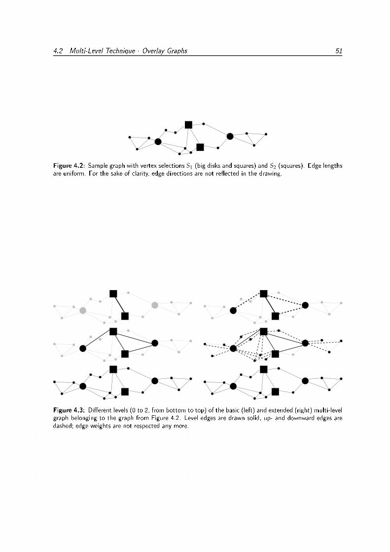
4.2 Multi-Level Te hnique · Overlay Graphs 51

Figure 4.2: Sample graph with vertex sele tions S1 (big disks and squares) and S2 (squares). Edge lengthsare uniform. For the sake of larity, edge dire tions are not re�e ted in the drawing.

Figure 4.3: Di�erent levels (0 to 2, from bottom to top) of the basi (left) and extended (right) multi-levelgraph belonging to the graph from Figure 4.2. Level edges are drawn solid, up- and downward edges aredashed; edge weights are not respe ted any more.

4.3 Multi-Level Te hnique · Shortest-Path Sear h 52

Cs0

Ct0

Cs1

Cs2

Cs3

Ct1

Ct2

Ct3

s t

Figure 4.4: Tree of onne ted omponents to the sample graph from Figure 4.2, with given verti es s andt. The Cs

0-Ct0-path is marked in red (k = k′ = 1 and Lst = 3).4.3 Shortest-Path Sear h

In this section we show how to use multi-level graphs to speed up single-pair shortest-path

algorithms. Depending on the given source and target vertices, a subgraph of the multi-

level graph is determined on which a shortest-path search is run. Since our approach es-

sentially defines another graph used as input for the actual computation, any shortest-path

algorithm can be used to perform the search. This is also the reason for which combina-

tions with other speed-up techniques that do or do not rely on precomputed information

are feasible (cf. [HSW04]).

We first revisit the definition of an auxiliary data structure called tree of connected com-

ponents, which is used in [SWZ02] to extract a suitable subgraph of an extended multi-level

graph. We demonstrate here only how to obtain, for a given query (s, t), a subgraph of a

basic multi-level graph in which the length of a shortest s-t-path remains unchanged, and

refer the reader to [SWZ02] for further details (in fact, both variants behave quite similarly).

We want to point out that computation of the subgraph and shortest-path search can be

performed in one pass, i. e., the subgraph is determined ‘on the fly’; a sketch of such a

routine is given at the end of this section.Tree of Conne ted Components. The subsequent definitions and employed notation are il-

lustrated in Figure 4.4.

4.3 Multi-Level Te hnique · Shortest-Path Sear h 53

Figure 4.5: For given verti es s and t, the subgraphsMst (left) andMst (right) of the basi and extendedmulti-level graphs from Figure 4.3.For 1 ≤ i ≤ l, consider the subgraph of G induced by V \ Si (we also use the rather

informal term of a decomposition of G). The set of connected components associated with

level i is then denoted by Ci, and for a vertex v ∈ V \ Si let Cvi denote the component in Ci

that contains v. For each component in C1∪ . . .∪Cl , there is a vertex in the tree; additionally,

there is a root Cl+1 corresponding to G and for every vertex v ∈ V a leaf Cv0 (our parlance

does not distinguish between a connected component and its belonging tree vertex, if the

context is unambiguous).

The parent of a vertex in the tree is determined as follows. For every component Cvi ∈ Ci

with 1 ≤ i ≤ l and v being an arbitrary vertex of that component, its parent is Cvi+1 (note

that component Cl+1 contains every vertex in V). For a leaf Cv0 , let j be the largest index

such that v ∈ Sj, or j := 0 if v /∈ S1; then the parent of Cv0 is Cv

j+1 (the smallest level where v

is contained in a non-singular connected component is j + 1).De�nition of the Subgraph. For given vertices s and t, consider the Cs0-Ct

0-path (Cs0, Cs

k, Csk+1,

. . . , CsLst

= CtLst

, . . . , Ctk′+1, Ct

k′ , Ct0) in the component tree, where Lst is the smallest index

with CsLst

= CtLst

(i. e., this component is the lowest common ancestor of Cs0 and Ct

0 ) and k

and k′ are the levels of the parents of Cs0 and Ct

0, respectively. This path induces a subgraph

Mst = (Vst, Est) of the basic multi-level graph M(G; S1, . . . , Sl): Est contains, for each

component Cxi on the path (x ∈ {s, t}, 0 < i < Lst), all edges in Ei−1 incident with a

vertex in Cxi , as well as all level edges ELst−1; the vertex set Vst is induced by Est. Figure 4.5

showsMst for our sample graph, and the subgraphMst of the extended multi-level graph

(cf. [SWZ02] for the definition) for reference.Shortest-Path Sear h. We now describe how to search for a shortest s-t-path in Mst using

the multi-level graph M (as mentioned above, Mst need not be extracted explicitly). We

4.3 Multi-Level Te hnique · Shortest-Path Sear h 54start from s at level k− 1 ofM, using edges in Ek−1. When a vertex in Sk is scanned, only

outgoing edges in Ek are taken into account, for vertices in Sk+1, only edges in Ek+1 and so

on. At level Lst − 1, all edges in ELst−1 can be visited. From a vertex in SLst−1 incident with

component CtLst−1, we ‘descend the hierarchy’, considering edges in ELst−2, and so on until

we reach t at level k′ − 1.

By definition of the component tree, any s-t-path must leave component Csk. Hence, it

suffices to maintain level-(k− 1) edges incident with vertices in Csk. The remaining part of

the shortest path can then be found from level-k vertices using higher-level edges. The same

argument applies iteratively for higher levels, and symmetrically for components around

t. At level Lst, vertices s and t belong to the same component, so all level-Lst−1 edges are

required. Summarizing, we can state (the strict proof is analogous to that in [SWZ02]):

Lemma 4.3.1. The lengths of shortest s-t-paths in G and inMst are equal.

4.4 Multi-Level Te hnique · Regular Multi-Level Graphs 554.4 Regular Multi-Level GraphsOne basic assumption for multi-level graphs to speed up shortest-path computation is that

the multi-level subgraphs are small compared to the original graph. In general, this is not

necessarily true; clearly, a bad example would be a set of vertices that does not decompose

the input graph at all.

However, for graphs that allow for some ‘regular’ decomposition we are able to prove,

for any (s, t)-query, a bound on the number of edges in the multi-level subgraph, which we

will show to depend crucially on the index Lst from the previous section. As this number

is mainly determined by the number of level-(Lst− 1) edges and the sets Ei get sparser as i

increases, we are also interested in the probability that for a random query at least a given

level Lst in the component tree is reached.

Note that the subsequent results refer to the extended version of multi-level graphs, but

can be carried over to the basic variant easily. For the sake of conciseness, we only outline

the main results, and refer the reader to [Hol03, Sch05] otherwise: proofs, which contain

rather lengthy but straightforward calculations, can be found there.

For experimental purposes, we also wish for graphs that permit a regular decomposi-

tion in the specified sense. A class of graphs that meet the theoretical results is therefore

described in the second part of this section.4.4.1 Theoreti al AnalysisAfter fixing some notation, we formally coin the notion of a regular decomposition, which

will serve as an assumption for all of the following considerations: First we bound the

number of edges in a regular multi-level graph, i. e., a multi-level graph exhibiting a regular

decomposition, then we note the probability that the highest level Lst on the path in the

component tree is at least some given value, and finally provide an upper bound on the

size of a multi-level subgraph.Notation. By EG(S) we denote the edge set induced by vertex set S in graph G. Further-

more, given a decomposition of G (with the same notation as in the previous section), the

maximal number of selected vertices adjacent to any vertex of any component in⋃l

i=1 Ci be

marked by a.

Definition 4.4.1. A decomposition of a graph G through vertex sets S1, . . . , Sl into connected com-

ponents⋃l

i=1 Ci is called regular if the number ∑li=1 |Ci| of all components is at most n and the

difference in the sets of edges induced by a consecutive pair of vertex sets is at least halved for two

consecutive pairs:

|EG(Si) \ EG(Si+1)| ≤ |EG(Si−1) \ EG(Si)|/2 (1 ≤ i < l).

4.4 Multi-Level Te hnique · Regular Multi-Level Graphs 56The size of the multi-level graph can be bounded as follows.

Lemma 4.4.2. Under the assumption of a regular decomposition, the total number of additional

edges in the multi-level graphM(G; S1, . . . , Sl) is at most

m + (a2 + a)n.

Let (s, t) ∈ V × V be a query selected uniformly at random. We want to give the

probability that the level Lst of the lowest common ancestor of Cs0 and Ct

0 in the component

tree is at least L (1 ≤ L ≤ l + 1).

Lemma 4.4.3. Under the assumption of a regular decomposition, the probability that for any vertices

s and t the index Lst is at least some L amounts to

2|SL−1|n− |SL−1|2 + (c− 1)(n− |SL−1|)2/c

n2 ,

if we suppose that all components in CL−1 have the same size c.

Let us further assume that c and the number |Sl | of vertices in the smallest subset are

constant. It follows that the probability with which the Cs0-Ct

0-path leads via the highest

level l converges to (c− 1)/c with n → ∞. Loosely speaking, with an apt decomposition

we can asymptotically expect to answer almost all queries by taking into account the top

level of the multi-level graph.

Finally, we are able to give a bound on the number of edges of the subgraphMst.

Lemma 4.4.4. Under the assumption of a regular decomposition, the total number of edges in the

subgraphMst is bounded by

2(a + (Lst − 2)a2) + |ELst−1|.

It turns out that a and |ELst−1| are the crucial parameters to the size ofMst. If a can be

considered a small constant, together with the above results we get that the search space

(number of edges in Mst) is asymptotically dominated by the number |El | of edges at the

highest level.4.4.2 Component-Indu ed Random GraphsMotivated by the above results, we now define a random graph model such that a reg-

ular decomposition is possible, component-induced graphs, which depend on the following

parameters:

• the number l′ of construction levels,

4.4 Multi-Level Te hnique · Regular Multi-Level Graphs 57

Figure 4.6: Sample omponent-indu ed graph with parameters l′ = 3, n′ = 5, m′ = 10, c′ = 3, a′ = 4.• the numbers n′ and m′ of new vertices and edges, respectively,

• the number c′ of new components per level, and

• the number a′ of adjacent vertices per component.

Construction of a component-induced graph is roughly done as follows (cf. [Sch05] for

further information). At top level, compute a classic Erdös-Réyni random graph with n′

vertices and m′ edges selected uniformly at random from all possible edges (cf. [Bol85]); if

it is not connected, repeat this step. The remaining l′ − 1 levels of the hierarchy are con-

structed in a recursive fashion: For the connected graph/component currently considered,

introduce c′ new connected components with n′ vertices and m′ edges each. From each of

these components, a′ (not necessarily distinct) vertices are picked and an edge from each of

these to some randomly selected vertex in the current component is introduced.

A regular decomposition of a component-induced graph can be obtained by including in

Si the vertices generated at levels greater than or equal to i + 1 with 1 ≤ i < l′. An example

of a component-induced graph with three construction levels is provided in Figure 4.6.

4.5 Multi-Level Te hnique · Experimental Analysis 584.5 Experimental AnalysisIn this section we give several criteria, along with two general strategies, of selecting vertices

of a graph to construct a multi-level graph, and introduce four graph classes investigated in

the subsequent experimental study. In a preparatory analysis we compare for given graphs

the multi-level graphs computed both by the min-overlay procedure and according to the

definition in [SWZ02]. In another prestudy we focus on two of the selection criteria that are

special in some sense, betweenness approximation and planar separator.

The main results show the impact of diverse combinations of graph class and selection

criterion and strategy on multi-level graphs as well as their performance when applied for

shortest-path search. Further experiments contrast basic and extended multi-level graphs

with different numbers of levels.

Our code is written in C++, based on the LEDA library [NM99], and compiled with

the GNU compiler (version 3.3); as underlying shortest-path routine we use Dijkstra’s algo-

rithm. The experiments were carried out on several 64-bit AMD Opteron machines, clocked

at roughly 2 GHz, with 4 or 8 GB of main memory.4.5.1 Sele ting Verti esIn the following, we present a variety of criteria of how to determine a subset of a graph’s

vertex set to construct a multi-level graph. All criteria—except for planar separator—can

be applied using one of two different selection strategies, global or recursive (the planar-

separator criterion can be applied only in a recursive manner).Sele tion CriteriaWe propose nine criteria: one random (RND) criterion; two criteria related to vertex degree,

degree (DEG) and percentage (PCT); one related to graph cores (COR) [BE05]; four com-

ing from centrality indexes, reach (RCH) [Gut04], closeness (CLO), betweenness (BET), and

betweenness approximation (BAP) [BE05]; and one involving a planar-separator algorithm

(PLS) [HPS+05].

Random (RND) Vertices are selected uniformly at random.

Degree (DEG) Vertices with the highest degrees are selected.

Percentage (PCT) We consider for each vertex v its percentage value, which is the share of v’s

adjacent vertices that have smaller degree than v in all adjacent vertices (an isolated

vertex is assigned −1). Vertices with the highest percentage values are then selected.

Core (COR) A graph’s k-core (for an integer k) is the maximal subgraph such that all ver-

tices in that subgraph have degree at least k. The core number of a vertex is defined

4.5 Multi-Level Te hnique · Experimental Analysis 59to be the maximum k such that this vertex belongs to the k-core. Vertices with the

highest core numbers are selected.

Reach (RCH) Reach r(v, p) of a vertex v on a path p is defined to be the minimum of the

lengths of p’s subpaths with respect to v. The reach of v is then the maximum of

all values r(v, p) where p is a shortest path passing by v, thus denoting the greatest

distance of v to the nearer of the end-vertices over all shortest paths containing v.

Vertices with the greatest reach values are selected.

Closeness (CLO) Closeness of v is defined as 1/

∑t∈V d(v, t) , letting d(v, t) denote the dis-

tance from v to t (with 1/0 := 0). Intuitively speaking, a vertex with great closeness

has short distances to most of the other vertices. Vertices with the largest closeness

values are selected.

Betweenness (BET) Betweenness of v is defined to be ∑s,t∈V σ(s, t | v)/

σ(s, t), where σ(s, t)

stands for the number of shortest paths from s to t and σ(s, t | v) for the number

of shortest paths from s to t that contain v as an internal vertex (with 0/0 := 0).

Betweenness reflects how important a vertex is to shortest paths. Vertices with the

greatest betweenness values are selected.

Betweenness Approximation (BAP) Betweenness can be approximated through random

sampling, by not taking into account all pairs (s, t) in V × V but only in V ′ × V ′,

for a subset V ′ ⊆ V of size (log n)/ε2 (with an appropriate choice of ε). The goal is

to obtain ‘good enough’ betweenness values in much shorter time than required for

computation of the exact values (cf. Section 4.5.4). The probability of an error larger

than εn(n− 2) is at most 1/n.

Planar Separator (PLS) This criterion makes use of Lipton and Tarjan’s planar-separator

algorithm described in Section 3.2.1, optimized for separator size. Since most of the

work on multi-level graphs was done at a rather early point in time, we were using

a heuristic suggested in [HPS+05], which simply draws a random sample of nodes

used for breadth-first search and returns the best separator thus induced.

In order to employ this criterion also for non-planar graphs, we first planarize the

graph by introducing new vertices at crossings (we presume a fixed embedding).

Then the planar-separator algorithm is applied to the planarized—auxiliary—graph.

Finally, separator vertices for the original graph are taken over from the auxiliary

graph, and conflicts with edges that connect two vertices of different components are

resolved by declaring one of the end-vertices a separator vertex (cf. Section 4.5.4).

Figure 4.7 illustrates the different criteria with a sample graph.

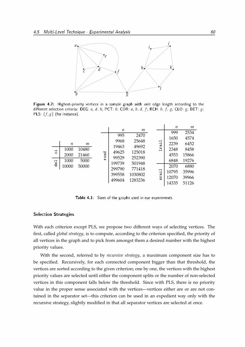
4.5 Multi-Level Te hnique · Experimental Analysis 60a

b

c d

e

f

g

h

ij

k

lFigure 4.7: Highest-priority verti es in a sample graph with unit edge length a ording to thedi�erent sele tion riteria: DEG: a, d, h; PCT: h; COR: a, b, d, f ; RCH: b, f , g; CLO: g; BET: g;PLS: { f , g} (for instan e).n m

1000 10480 i 2000 214601000 5000del 10000 50000

n m

995 24709968 25648

19463 4969249625 12501899529 252390

199739 501948299790 771418399558 1030802

road499604 1283236

n m

999 25341650 45742239 64522348 84584553 15866

lrail6848 192762070 6880

10795 3599612070 39966srail14335 51126Table 4.1: Sizes of the graphs used in our experiments.Sele tion Strategies

With each criterion except PLS, we propose two different ways of selecting vertices. The

first, called global strategy, is to compute, according to the criterion specified, the priority of

all vertices in the graph and to pick from amongst them a desired number with the highest

priority values.

With the second, referred to by recursive strategy, a maximum component size has to

be specified. Recursively, for each connected component bigger than that threshold, the

vertices are sorted according to the given criterion; one by one, the vertices with the highest

priority values are selected until either the component splits or the number of non-selected

vertices in this component falls below the threshold. Since with PLS, there is no priority

value in the proper sense associated with the vertices—vertices either are or are not con-

tained in the separator set—this criterion can be used in an expedient way only with the

recursive strategy, slightly modified in that all separator vertices are selected at once.

4.5 Multi-Level Te hnique · Experimental Analysis 61

Figure 4.8: Sample planar Delaunay graph.4.5.2 Graph ClassesWith our experiments we take into account four types of graphs, two randomly generated

and two taken from real world. All graphs are connected and bidirected, i. e., as the case

may be, each edge has been replaced with two directed edges, one in either direction. For

each of the subsequent graph classes we provide a short key, which can be further specified

by the number of vertices to denote a concrete instance. Table 4.1 provides a synopsis of

the graph sizes.

Component-Induced Graphs ( i) Due to construction (cf. Section 4.4.2), these random

graphs exhibit some regular hierarchical structure and are rather dense compared

to the other classes. Edge lengths are chosen at random.

Planar Delaunay Graphs (del) Planar Delaunay graphs are graphs with vertices randomly

spread over a unit square for which the Delaunay triangulation is computed. Then

edges are deleted at random until a given number is reached. We chose the number

of edges such that density ranges somewhere between the values for the i and real-

world graphs. Edge lengths correspond to Euclidian distances.

Road Graphs (road) By road graphs we denote subgraphs of the German road network.2

These graphs are comparatively sparse. The length of an edge is the length of the

corresponding road section—not the straight-line distance—with a granularity of 10

meters. For our experimental study, we use road graphs with up to roughly 500 000

vertices.

2We are grateful to the ompanies PTV AG, Karlsruhe, and HaCon, Hannover, for providing us with road andrailway data, respe tively.


Figure 4.9: Re ursive de ompositions of srail2070 (lo al bus servi e network in entral Germany),lrail6848 (railway network of Germany), and road19463 (road network of Karlsruhe and surroundingarea) by PLS. The bla k squares mark the separator verti es, di�erent omponents are indi ated by olors.Railway Graphs (rail) Railway3 graphs are condensed networks reflecting train connec-

tions2 (cf. [SWW00]): vertices stand for railway stations, and there exists an edge

between two vertices if there is a non-stop connection between the respective stations.

As opposed to road graphs, which are almost planar, specimens of this class can have

quite some edges spanning a major distance. Graphs representing long-distance traf-

fic within some European countries (lrail) or local/short-distance transportation of

several German regions (srail) are provided. The length of an edge is assigned the

average travel time of all trains that contribute to this edge. The lrail graphs contain

up to almost 7000 vertices, while there are approximately twice as many in the largestsrail graph.

Sample instances of these graph classes can be found in Figures 4.6, 4.8, and 4.9, respec-

tively. The generator for the i and del graphs is available on-line [BGH+05].4.5.3 Shortest-Path Overlay GraphsIn Theorem 4.2.2 we proved that the procedure min-overlay yields shortest-path overlay

graphs with a minimal number of edges. To get an idea of the amount of edges that can be

saved when switching from the definition in [SWZ02]4 to the minimal variant given in this

work, we compare for one graph of each class the sizes of (extended) multi-level graphs

3Note that terms like railway, train, et . here omprise also other means of publi transportation, su h as trams,lo al buses and so on.4The pro edure in [SWZ02℄ di�ers from min-overlay in one fundamental respe t: When two shortest pathsof equal length are en ountered, one of them is pi ked arbitrarily to be in luded in the multi-level graph. This mayresult in di�erent potential multi-level graphs so for our omparison, we onsider one with a maximal number ofedges.

4.5 Multi-Level Te hnique · Experimental Analysis 63unit lengths genuine lengths

graph opt blowup opt blowup i2000 7.0 1.21 6.9 1.00del10000 31.1 2.95 35.4 1.00road19463 12.6 1.26 15.8 1.01rail6848 5.9 1.37 8.8 1.00Table 4.2: Comparison of multi-level graphs omputed through min-overlay and a ording to [SWZ02℄.opt denotes the number of edges divided by the number of verti es obtained with min-overlay, whileblowup indi ates the multipli ative fa tor indi ating how many edges in relation are onstru ted using thenon-minimal method. We distinguish the ase of unit (left) and genuine (right) edge lengths.obtained by either procedure (induced by one subset of vertices each, determined with

PLS). Moreover, we provide two different kinds of edge lengths: genuine ones, as described

above, and unit lengths.

The outcome is depicted in Table 4.2: opt denotes the number of edges divided by the

number of vertices in the minimal overlay graph and blowup the quotient of the numbers

of edges obtained with each procedure. Under the use of unit lengths, there exist many

paths of equal length, resulting in a comparatively big blowup (almost 3 for the del graph)

while with genuine lengths, there is practically none. The latter observation is owed to the

fact that edge lengths are Euclidean lengths or mean travel times, represented by double-

values, so it is rather unlikely that different paths between two vertices have equal length.

If actual, integer-valued travel times were used for the rail graph instead, we would expect

a blowup factor lying between the two given in the table.4.5.4 Spe ial Sele tion CriteriaMost of the criteria described in Section 4.5.1 are uniquely determined. However, BAP

involves parameter-dependent random sampling, where an appropriate choice of the pa-

rameter for our purposes cannot be given offhand. Moreover, PLS applied to non-planar

graphs requires planarization and retranslation steps, where effects on the size of the selec-

tion set remain quite unclear. These issues are highlighted in the following prestudies.Betweenness ApproximationTo assess the quality of betweenness approximation and to earmark a parameter setting

for practical application, we determine for different choices of ε vertex selection sets and

investigate the average search space size of belonging multi-level graphs: For a fixed maxi-

mum component size, we construct extended multi-level graphs of road49463, induced by

both exact and approximated betweenness, and with each of these graphs answer a series

of shortest-path queries. We then evaluate the number of visited edges, i. e., scanned by the


46

810

1214

0.0 0.5 1.0 1.5 2.0Figure 4.10: Quotient of the average numbers of edges visited during shortest-path omputation withmulti-level graphs based on BAP and BET. The abs issa denotes the parameter ε, governing the randomsampling. As input graph, road49463 is used.shortest-path algorithm.

Figure 4.10 shows the ratio of the numbers of visited edges with approximated and

exact betweenness values, for choices of ε of up to 2: the larger this ratio, the smaller is

the speed-up achieved with BAP. We observe that with increasing ε, performance of the

multi-level approach at first worsens only very slowly but for ε ≥ 1, slumps dramatically.

For subsequent experiments with BAP, we want to play safe by setting ε to a value

of only 0.2. Nevertheless, this leads to a drastically reduced preprocessing time of about

0.5 % of that needed to compute exact betweenness. Further tests with other road graphs

confirmed this choice of ε as appropriate.Planar SeparatorAs mentioned in Section 4.5.1, our planar-separator algorithm can be applied also to non-

planar graphs: Planarize the input graph by introducing a vertex for each crossing, run the

separation algorithm, and retranslate the separator found to the original graph by possibly

including further vertices in the separator set. Afterwards, a simple procedure can be used

to optimize the separator set by sorting out ‘redundant’ vertices. The main issues that we

want to cover in this prestudy are: the number of crossings in the input graph (and thus

the number n∗ of planarization vertices) and the size |Sopt| of the separator set induced for

the original graph. We respect road and lrail graphs, with maximum component sizes of

500 and 1000.

The results are depicted in Table 4.3, showing for each graph the number of crossings as

well as the separator sizes (for the planarized graph, the original graph, and after optimiza-

tion). As alluded above, the road graphs are already almost planar, which is not true for

the rail graphs. This is underpinned by the values for n∗, ranging around 2 percent of the

4.5 Multi-Level Te hnique · Experimental Analysis 65graph n∗ |S∗| |S| |Sopt|road19463 479 165 196 177road49625 1060 336 410 382road99529 2591 773 941 855road199739 3754 2176 2636 2315road299790 8025 3399 4104 3628lrail1650 645 22 38 16lrail2239 1830 68 107 55lrail2348 3458 154 132 58lrail4553 11447 605 412 164lrail6848 3169 183 399 164Table 4.3: Appli ation of the planar-separator algorithm to non-planar graphs (road and lrail). Thefollowing measurements (average values with di�erent maximum omponent sizes) are re�e ted: number

n∗ of rossings in the input graph/planarization verti es, size |S∗| of the separator for the planarized graph,size |S| of the retranslated separator, and size |Sopt| of the separator for the input graph after removal ofredundant verti es.number of original vertices for road graphs, but between 39 and an enormous 251 percent

for lrail. The optimized separator sets, Sopt, however, are quite small for both classes,

consisting of roughly 1 percent and up to 3.6 percent of vertices in the input graph, respec-

tively. For further experiments, this outcome suggests the feasibility of a decomposition of

our real-world graphs by PLS through a ‘reasonable’ number of vertices.

One alternative to the planar-separator algorithm is the graph-partitioning tool METIS

[Kar95], which computes balanced edge partitions rather than vertex separations (from an

edge partition, a vertex separator can be derived by a simple greedy heuristic). In [HPS+05],

it is shown that separators obtained through METIS are of almost the same quality (with

respect to both separator size and component balance) as those received by our planar-

separator algorithm. Preliminary experiments corroborate that this observation carries

over to the multi-level approach in that performance with selected vertices determined

via METIS is slightly worse than with PLS-computed selections.4.5.5 Multi-Level Approa hThis section contains a computational study in which we investigate the performance of

the multi-level approach with different parameters: We consider diverse combinations of

graph class, selection criterion and strategy, and number of levels, as well as contrast the

basic and extended versions. Our experiments are divided into three sections: first, we

focus on extended multi-level graphs and explore different combinations of settings, but

restrict ourselves to only one additional level; then we compare basic multi-level graphs to

the extended variant; finally, we factor multiple levels into our experiments.

As the most important measure for speed-up we use the quotient of the number of edges

4.5 Multi-Level Te hnique · Experimental Analysis 66visited by Dijkstra’s algorithm over that number visited by the search routine of the multi-

level approach. This parameter is implementation- and machine-independent, and turned

out to be closely related to CPU time.Sele tion CriteriaWe explore all combinations of graph type, selection criterion, and number of selected ver-

tices or maximum component size, respectively (due to the large number of combinations,

we have to settle for rather small graphs). According to these results, we pick in a second

pass the most promising parameter settings to run them with a series of larger graphs,

where we take a closer look at the influence of the maximum component size.Small Graphs. We take into account one graph of each type with about 1000 vertices: i1000, del1000, road995, and lrail999. With the global strategy, we choose for the num-

ber of selected vertices 3, 5, 8, and 10 percent of the number of vertices in the graph and

with recursive decomposition, the maximum component size is set to 3, 5, 10, and 20 per-

cent, which in some preliminary runs turned out to be representative values. For each of

these combinations, we run 1000 queries selected at random and compute the averages of

the resulting speed-up values.

Figure 4.11 presents average speed-up in the form of standard boxplots: Each box spans,

for one criterion and one graph, the range obtained with the four choices for the number

of selected vertices and the maximum component size, respectively. Overall, the highest

speed-up values are obtained with recursive BET/BAP (there is hardly any difference be-

tween these two criteria; cf. Section 4.5.4), which work very well for all graphs but del1000;

a factor of almost 20 can be achieved with road995. The second-best criterion, of similar

quality, turns out to be PLS, followed by recursive RCH. The DEG criterion suitably decom-

poses lrail999, which can be explained by the large range of vertex degrees compared to

other graphs. Some of the other criteria work only slightly better than selection by RND. In

general, with recursive decomposition higher speed-ups are attainable.

As for graph classes, del constitutes a hard instance, whereas for the real-world and i graphs the approach is well-suited. For i1000, recursive BET/BAP yields a maximal

speed-up of around 10, which quite corresponds to the value obtained with a multi-level

graph induced by the vertices selected during construction of the input graph. Analyz-

ing for global and recursive decomposition the variability of the component sizes and the

number of selected vertices in the multi-level graphs, respectively, a strong correlation to

the speed-up values becomes evident: the smaller component size variance and selection

set, the better the speed-up. Note that these results parallel our deliberations on regular

decomposition in Section 4.4.


BET BAP CLO COR DEG PCT RCHRND

05

1015

20

BET BAP CLO COR DEG PCT PLS RCHRND

05

1015

20

Figure 4.11: Speed-up in terms of visited edges with global (left) and re ursive (right) de omposition.The x-axis denotes the sele tion riterion; graphs onsidered (from left to right within ea h riterion): i1000 (white), road995 (dark-gray), lrail999 (light-gray), and del1000 (brown). The boxplots spanthe average speed-up values with di�erent hoi es for the number of sele ted verti es (3, 5, 8, and 10per ent) and the maximum omponent size (3, 5, 10, and 20 per ent), respe tively. The horizontal linewithin a box denotes the median, the ross marks the mean value.


1015

2025

30

10 20 50 100

1015

2025

10 20 50 100Figure 4.12: Average speed-up with PLS (left) and re ursive BAP (right) for larger road graphs. Thex-axis denotes the number of verti es in the input graph (in thousands). Maximum omponent sizes: 1(solid), 10 (dashed), and 20 (dotted) per ent.0

510

1520

5 10 15 0

34

56

78

5 10 15Figure 4.13: Average speed-up with extended (left) and basi (right) multi-level graphs of rail graphs.The x-axis denotes the number of verti es in the input graph (in thousands). Maximum omponent sizes:10 per ent for the extended and 1 per ent for the basi multi-level graphs; sele tion riteria: re ursive DEG(solid) and PLS (dashed); graph lasses: lrail ( ir le) and srail (triangle).Medium-Size Graphs. With a series of somewhat larger real-world graphs and the most

promising criteria identified in the previous paragraph, we again run random queries with

different maximum component sizes. We use recursive BAP and PLS for the road as well

as recursive DEG and PLS for the rail graphs.

Figure 4.12 shows the speed-up for road graphs with up to 100 000 vertices. For the

largest graph, a speed-up factor of 31 is reachable. Here, the PLS criterion is clearly superior

to BAP, with which the maximal speed-up is 22. For the maximum component size, 10

percent turns out to be the best choice. Concerning preprocessing times, decomposition ofroad99529 takes several minutes with PLS, but around two hours with BAP. Times for the

construction of the multi-level graph, of well over half an hour, are similar for both criteria.

According to these findings, we settle for a maximum component size of 10 percent forrail graphs, but distinguish between long- and short-distance networks (cf. Figure 4.13,

left). Interestingly, for lrail graphs, DEG works better than PLS while for srail, speed-up

with DEG is not very pronounced, whereas PLS yields much higher factors.

4.5 Multi-Level Te hnique · Experimental Analysis 691.

01.

21.

41.

61.

82.

02.

2

10 20 50 100

24

68

1012

10 20 50 100Figure 4.14: Relative average speed-up with extended (left) and basi (right) multi-level graphs of roadgraphs. The x-axis denotes the number of verti es in the input graph (in thousands). Maximum omponentsizes: 1 (solid), 10 (dashed), and 20 (dotted) per ent; sele tion riterion is PLS.Basi Multi-Level GraphsThe main feature that distinguishes basic from extended multi-level graphs is that no up-

ward and downward edges are maintained (cf. Section 4.2.2). Hence, one may expect more

edges that have to be visited during a search and thus less speed-up; at the same time, the

overhead of storing additional edges is smaller. This notion is captured by relative speed-

up, which is defined as speed-up divided by graph expansion, where graph expansion is

the quotient of the numbers of edges in the multi-level and the original graph. We run

experiments with the same medium-sized road and rail graphs as above.

Figure 4.14 depicts relative speed-up for the road graphs with both extended and basic

multi-level graphs and the PLS criterion. The best value observed with the extended version

is about 2.3, but well over 12 with the basic. Graph expansion of basic multi-level graphs

is only slightly greater than 1, so the right-hand diagram shows at the same time virtually

pure speed-up and can thus be perfectly compared to Figure 4.12: best speed-up is obtained

with a maximum component size of 1 percent, in contrast to 10 percent for the extended

version. This suggests that the maximum component size should be chosen smaller for

basic multi-level graphs (with respect to relative speed-up, however, 1 percent seems to

be advantageous for both variants). Finally, the right-hand diagram in Figure 4.13 reflects

speed-up with basic multi-level graphs of rail graphs.Multiple LevelsThe last series of experiments is devoted to the question of how much speed-up can be

gained by introducing more than one level, where we use medium-sized and large road (cf.

Table 4.1) as well as larger i graphs.Road Graphs. We consider three-level extended and basic multi-level graphs of road99529,

based on different combinations of vertex selections through PLS. Figure 4.15 shows that


3540

4550

5 10 15 20

1516

1718

1920

2122

5 10 15 20Figure 4.15: Average speed-up with extended (left) and basi (right) multi-level graphs of road99529with two additional levels. The x-axis denotes the maximum omponent size (in thousands of verti es)for level 1; maximum omponent sizes for level 2: 300 (solid), 500 (dashed), 1000 (dotted), and 1500(dotted-dashed) verti es; separation riterion is PLS.speed-up can be increased from 31 with one level (cf. Figure 4.12) to well over 50 (with

maximum component sizes of 15 and 3 to 5 percent) and from about 13 (cf. Figure 4.14)

to 22 (with 5 and .3 percent) using extended and basic multi-level graphs, respectively. A

similar behavior could be observed with even larger road graphs: not only could speed-up

be improved by introducing another level; also, with extended multi-level graphs, graph

expansion could be reduced drastically while for basic multi-level graphs, it appeared to

still be negligible.Component-Indu ed Graphs. Last, we want to refer to [Hol03] for an experimental study in-

vestigating component-induced graphs with up to 100 000 vertices and belonging extended

multi-level graphs with up to five additional levels, where vertices used during construc-

tion of the input graphs are selected. The main outcome is that with increasing graph

size, speed-up scales to a factor of approximately 1000. These results further confirm the

intuition and results from Section 4.4, viz., importance of a regular decomposition.SummaryWe want to conclude our empiric study by extracting from the above experiments some

principal insights, which can be seen as a guideline to choosing good parameter settings

for multi-level shortest-path computation. Concerning selection criterion, we would recom-

mend PLS or recursive BAP5, or recursive DEG for real-world graphs with a great variance

of vertex degrees. Storage capacity permitting, the extended variant should be favored over

the basic (where the latter allows for unbeatable relative speed-up), with a maximum com-

ponent size of around 10 percent of the vertices in the input graph. For graphs with more

than 1000 vertices, employing two or even more levels should be considered.

5In our experiments, BAP may have in urred greater prepro essing times, but this defe t ould be over ome bya more ourageous hoi e of ε, with little loss in speed-up.

4.6 Multi-Level Te hnique · Dis ussion 714.6 Dis ussionIn this study, we further developed the multi-level technique for shortest-path compu-

tation through several steps of refinement: we improved the definition of shortest-path

overlay/multi-level graphs, introduced a new—the basic—variant, and provided several

criteria along with two general strategies to select vertices in a graph for construction of

multi-level graphs. The theory part provides some common considerations regarding the

speed-up that can be achieved given a regular decomposition of the input graph.

In an extensive experimental study, both variations of multi-level graphs were tested

for shortest-path speed-up, along with different selection criteria and strategies as well as

various random and real-world graphs. Results have shown:

• The recursive decomposition strategy allows for a more balanced distribution of con-

nected components and thus performs better than the global one.

• Regarding selection criteria, planar separator and betweenness clearly outdid the oth-

ers. Further, betweenness was shown to be approximated efficiently. Also, the degree

criterion sped up shortest-path computation with long-distance rail graphs.

• Comparing the two variants in terms of mere speed-up, extended multi-level graphs

are superior to basic ones; however, the latter turned out to be more efficient when

multi-level graph size was taken into account.

Several measures to further enhance the multi-level technique have already been taken

developing the high-performance multi-level and the transit / highway node routing tech-

niques (cf. Section 4.1.1). The most important changes made towards the high-performance

variant concern heavier precomputation of shortest-path information as well as distribution

of the multi-level graph to many partial graphs, which allows for individual optimization.

In comparison to highway node routing, a major difference is constituted by the altered

selecting strategy by means of a highway hierarchies precomputation. Such a selection

turns out to be comparatively sparse, virtually not decomposing the input graph, which

requires a different search routine: the latter has the advantage that shortest-path search

is not necessarily restricted to one level at a time, but vertices belonging to different levels

may be considered in parallel.

Despite these recent developments, subjects remaining for future research include:

• The vertex selections computed for this study through the PLS criterion rely on a

rather early stage of our planar-separator implementation. Since that code has been

embellished with some more recent features mentioned in the previous chapter, and

separator quality could be significantly improved for many cases, it would be in-

teresting to reevaluate the impact on multi-level overlay graphs and shortest-path

speed-up.

4.6 Multi-Level Te hnique · Dis ussion 72• As pointed out in Section 4.1.1, the issue of dynamizing the multi-level technique has

been addressed from a theoretic standpoint in [Bau06], as well as in some very recent

work [BCD+08], while to our knowledge no empiric evaluation of these ideas has

been conducted.

Chapter 5Multimodal RoutingThe multimodal shortest-path problem constitutes a generalization of the standard, or uni-

modal, shortest-path problem, considered in the previous chapter. Each edge of a given

graph is additionally assigned some label. We can now formulate different kinds of con-

straints on shortest paths in this graph through formal languages constructed upon these

labels. In the subsequent investigation, we settle for regular languages, which represent

both a powerful and computationally feasible class of restrictions. This model covers a di-

verse collection of shortest-path-related problems, many of them highly relevant in traffic-

planning, especially in connection with multiple modes of transport.

In contrast to the previous problem, this variant has by far less been studied. With the

former, the focus of research has, over the intervening years, shifted to fairly sophisticated

speed-up techniques or issues of dynamization (cf. Section 4.1.1). In line with what we said

in Chapter 2, it is necessary for the multimodal case to go back to the more basic concepts:

our goal is a thorough evaluation of algorithms applied to different scenarios with a range

of typical inputs. The primary contribution is to analyze how several well-known speed-up

techniques for the unimodal shortest-path problem can be adapted to solve the constrained

variant in view of practical applications.

To this end, we implemented adaptations of Dijkstra’s shortest-path algorithm as well

as of several speed-up techniques, and conducted an extensive experimental study using

realistic transportation networks and language constraints. Experiments show that some of

the insights gained from the unimodal setting can be carried over, while others differ. We

further suggest ways of enhancing other promising speed-up techniques to be used in the

multimodal scenario.

5.1 Multimodal Routing · Overview 74

Figure 5.1: Clipping of the KVV publi -transportation network (showing Karlsruhe ity enter). Red,green, dark-gray, and purple lines represent the street ar, rapid-transit railway (S-Bahn), regional train, andbus systems, respe tively; ar-sharing fa ilities are also indi ated [ ℄.5.1 OverviewIn this preliminary section, we want to motivate the relevance of the given topic in everyday

applications, outline our proceeding of investigating this problem, and give a synopsis of

other work done in the context of constrained-shortest-path computation.5.1.1 MotivationIn vehicle routing and urban transport-planning, different kinds of multimodal traffic net-

works are widely used, where roads may be differentiated by categories (highways, primary

roads/arterials, local streets, etc.), or there are several means of transportation involved.

One common task is to find in such a network a shortest path from a given start to a des-

tination vertex so that the use of road categories and means of transportation, respectively,

follows some desired pattern: e. g., a truck driver in Germany or other European countries

may want to renounce highway usage in order to avoid toll fees, or a car driver who is pre-

pared to use park-and-ride facilities may consider routes that include the modes of travel

car, public transportation, and walk. As an example of multimodal information, Figure 5.1

shows parts of the map representing the Karlsruhe public-transportation1 network.

Other problems arising in the context of vehicle routing include

1Karlsruher Verkehrsverbund (KVV); http://www.kvv.de.

5.1 Multimodal Routing · Overview 75• the k-similar-path problem, where we want to compute two shortest paths between the

same pair of vertices such that the second path reuses at most k edges of the first

one. This is a task that an on-board navigation system might have to solve when

suggesting alternate routes to avoid traffic jams.

• turn limitation problems, which deal, e. g., with finding a shortest path that avoids

left turns at intersections with heavy traffic in order to save travel time (we are told

that UPS America tries to route its pick-up trucks this way to improve efficiency2).

To formalize all these problems, we augment the network edges with appropriate labels

and model the path restriction as a formal language; the labels of the edges on a shortest

path must then form an element of the language. More formally, given an alphabet Σ, a

graph—or network3—G whose edges are weighted and Σ-labeled, and a regular language

L ⊆ Σ∗, the L-constrained shortest-path problem (LCSP) consists in finding a shortest path p

in G such that the word obtained by concatenating the labels on the edges comprising p

belongs to L. We will see in Section 5.2.3 how to express some of the above-mentioned

constraints as a formal language.

A detailed theoretic study of formal-language-constrained shortest-path problems for a

variety of constraining languages was undertaken in [BJM00]. It is shown that the regular-

language-constrained shortest-path problem (RegLCSP) is efficiently solvable in polynomial

time. The algorithm proposed makes use of the fact that each regular language can be

represented by a nondeterministic finite automaton (NFA), and constitutes a generalization

of Dijkstra’s algorithm, which operates on a product network composed of the input graph

and a respective NFA. Regular languages have proven to be comprehensive enough to cover

a broad range of interesting applications. In [BBJ+02], an algorithm for the special case of

linear languages (LinLCSP) is empirically evaluated.

Building on this earlier work, we consider here the full RegLCSP problem. We describe

a practical way of implementing the algorithm suggested in [BJM00], and adapt several

elementary techniques designed to give reliable speed-up for the standard shortest-path

problem, viz., goal-directed search, Sedgewick-Vitter heuristic, and bidirectional search as well as

combinations of these. The experimental part of our study explores applicability of these

algorithmic variants to diverse real-world transportation networks, including two different

applications; scalability is tested by employing instances of increasing size and language

constraints of varying complexity (both linear and general regular expressions). Finally,

we analyze some more of a great many speed-up techniques in the context of multimodal

routing, which nevertheless remains a wide field for further research.

2Cf. http://telstarlogisti s.typepad. om/telstarlogisti s/2007/03/how_ups_will_sa.html.3In this hapter, the terms graph and network are used synonymously.

5.1 Multimodal Routing · Overview 765.1.2 Related WorkResearch on generalizations of the standard shortest-path problem has traditionally fo-

cused on the extension of Dijkstra’s algorithm [Dij59] to time-dependent cost functions

(e. g., [OR90]) or on dynamic aspects, such as deletion or insertion of edges or change of

edge weights (e. g., [DI06, SS07]). In contrast, comparatively little work has been done

on constraints restricting the set of feasible paths. It is important to note that our label-

constrained problem is not to be confused with the (resource-)constrained shortest-path vari-

ant (cf. [KMS05]), where, in addition to lengths, edges are assigned costs and the total cost

of a shortest path must not exceed a given bound.

In transportation science and operations research literature, there are reports on stud-

ies of multimodal, or intermodal, shortest paths (e. g., [LS01, MS98]). However, there are

two fundamental differences to our investigation, regarding both scope of application and

experimental proceeding:

• The main concern of those works is to study the multimodal problem with a concrete

scenario, typically arising from regional transportation problems, where the applica-

tions are mostly limited to certain travel mode schemes; sometimes, the given task

involves multiple criteria, i. e., finding a shortest path with respect to some tradeoff

between different factors like travel time, cost, and the number of changes. Although

for specific scenarios, some of the custom-tailored procedures proposed there may be

more efficient than the algorithms presented in this work, our endeavor is to develop

more general proceedings with a broader range of applications.

• Experiments conducted in those studies are often limited in that just one—or very

few—networks are tested, many of which are also substantially smaller than ours,

and combinations of different networks, parameter settings, etc. are explored rather

sparingly. In contrast, we strive to carry out an inductive evaluation as exhaustive as

possible.

An extensive study of a variety of traffic-planning problems under the use of real-world

data has been done in the TRANSIMS project [BBS+95, BBH+07]. Regular languages as

a model for constrained-shortest-path problems were first suggested in [Rom88]. Apart

from issues in the realm of traffic-planning, further applications of multimodal routing

include Web search and database queries (cf. [Yan90, MW95], and [BJM00] for a more

comprehensive survey).

We now focus on several pieces of preceding work that are strongly related to ours:Theoreti Work. A theoretic survey [BJM00] gives an overview of formal-language-

constrained shortest-path variants with respect to problem complexity for different classes

5.1 Multimodal Routing · Overview 77of restricting languages. Both regular and context-free languages are shown to permit poly-

nomial algorithms: an efficient algorithm suggested for the former class is also used in this

work. Moreover, the paper provides a collection of problems that can be tackled using

formal languages, two of which are investigated here from an application point of view.Linear Expressions. In [BBJ+02], an adaptation of Dijkstra’s algorithm to the LinLCSP prob-

lem with time-dependent edge weights obeying the FIFO property is given: this algorithm

relies on an implicit representation of the given language constraint, which, however, does

not involve finite automata as in our case, but employs an array (cf. Sections 5.2.2 and 5.5

for more information). As for speed-up techniques, both goal-directed search and the

Sedgewick-Vitter heuristic are empirically tested on a road network with a few hundred

thousand vertices: it is shown that by choosing for the Sedgewick-Vitter heuristic an ‘ap-

propriate’ overdo factor (corresponding to the α-parameter in Section 5.3), running time

can be increased considerably with little loss in path quality (cf. Section 5.4.2).Time Dependen e. Two recent works [SJH03, SJH06] consider the RegLCSP problem for

FIFO weight functions: [SJH03] presents an implicit, dynamic-programming-based algo-

rithm, which is extended in [SJH06] to allow for turn penalties. The latter work also gives

an adaptation of Dijkstra’s algorithm closely related to the one used in this work. For both

algorithms, several curtailing heuristics are proposed, which mostly make use of geometric

graph information. Experiments investigating diverse combinations of base algorithm and

speed-up heuristic are executed for two kinds of US transportation networks. Other im-

portant differences to our study include the facts that the networks of up to 4000 vertices

are substantially smaller than ours, and no systematic analysis of language constraints is

provided.

5.2 Multimodal Routing · Foundation 785.2 FoundationIn this section, we formally define the regular-language-constrained shortest-path problem,

show how it can be solved using product networks, and in more detail describe the two

applications used with our experiments.5.2.1 Problem StatementGiven a finite set Σ, called alphabet, of elements denoted as symbols or letters4, a formal

language over Σ is a subset L ⊆ Σ∗, where Σ∗ consists of all finite concatenations—or

words—of symbols in Σ. The class of regular languages can be described inductively:

Definition 5.2.1 (Regular Language). Each singleton set {a} with a ∈ Σ as well as the set

consisting of only the empty word ε are regular languages. For any regular languages L1 and L2,

• the union L1 ∪ L2,

• the concatenation L1 · L2 := {w1w2 := w1 ·w2 | w1 ∈ L1, w2 ∈ L2}, and

• the Kleene closure L∗1 := {w ·w · · ·w︸︷︷︸

k times

| w ∈ L1, k ∈ N0}

are also regular languages. For convenience, the positive closure, L+1 , analogously denotes ‘non-

empty repetition.’(Often a regular language is noted by its regular expression, e. g., (a ∪ b)∗c

instead of ({a} ∪ {b})∗ · {c}.)

Based upon this definition, we can now formulate the regular-language-constrained

shortest-path problem.

Definition 5.2.2 (RegLCSP). Given an alphabet Σ, a graph G = (V, E, c, ℓ) with cost5 function

c : E → R+0 and labeling function ℓ : E → Σ, and a regular language L ⊆ Σ∗. For a query

of source and destination vertices (s, d) ∈ V × V, find a shortest s-d-path p with edge sequence

〈e1, e2, . . . , ek〉 in G such that ℓ(p) ∈ L, where ℓ(p) is the concatenation ℓ(e1) · ℓ(e2) · · · ℓ(ek). The

cost of p is the sum of costs of p’s edges.

It is obvious that any shortest s-d-path subject to any restriction is at least as long as a

shortest unrestricted s-d-path.NFA. By Kleene’s theorem, each regular language L ⊆ Σ∗ can be represented through a

nondeterministic finite automaton (NFA) A = (Q, Σ, δ, q0, F) with set Q of states, transition

function δ, start state q0, and set F of final, or accepting, states. A word w ∈ Σ∗ is contained

in L if and only if there is a sequence of transitions in A from q0 to any final state with

corresponding label sequence equal to w. Further, A has a canonical graph representation

with a vertex for each state and a labeled edge for each transition (cf. below).

4In our ontext, they are also referred to as labels.5In the following, the terms ost, weight, and length are used inter hangeably.

5.2 Multimodal Routing · Foundation 79Vertex Labels. Instead of employing edge labels, it would also be possible to assign a label

to each vertex. One application relying on this kind of labeling is trip chaining, where

a shortest path is searched such that it contains a sequence of intermediate vertices with

given labels (this model covers, e. g., certain ‘errand-running problems’). In this work, we

restrict ourselves to edge labels. However, it is shown in [BJM00] that vertex labels can

be emulated by edge labels fairly easily: the idea is to label all edges with the same, new

symbol, and attach to each vertex a loop labeled with the symbol of that vertex; roughly

speaking, the constraint has to be altered by inserting the new symbol between any two

original symbols.5.2.2 Produ t NetworkThe central feature of the RegLCSP algorithm described in [BJM00] is the use of a product

network constructed from the given graph and an NFA encoding the language constraint.

Definition 5.2.3 (Product Network). Given a weighted, Σ-labeled digraph G = (V, E, c, ℓG), an

NFA A = (Q, Σ, δ, q0, F) encoding some language L ⊆ Σ∗, and let further be T the set of state

transitions t = (q1, q2) with q2 ∈ δ(q1) and labels ℓA(t) ∈ Σ. The product network P = G× A is

defined to have vertex set {(v, q) | v ∈ V, q ∈ Q} and edge set {(e, t) | e ∈ E, t ∈ T, ℓG(e) =

ℓA(t)}. The cost of an edge (e, t) ∈ P corresponds to c(e).

The RegLCSP algorithm relies on the fact that there is a one-to-one correspondence

between s-d-paths in G whose labeling belongs to L and paths in P starting at (s, q0) and

ending at some vertex (d, f ) with f ∈ F, and thus performs a shortest-path search in P:

Theorem 5.2.4. Finding an L-constrained shortest path for some L ⊆ Σ∗ and (s, d) ∈ V × V is

equivalent to finding a shortest path in the product network P = G× A from vertex (s, q0) to (d, f )

for some f ∈ F.5.2.3 Appli ationsFor our experiments, we consider the following two applications of the RegLCSP.

Multimodal Plans. Consider a traveler who wants to take a bus from a start s to a destina-

tion point d and suppose transfers are undesirable, while walks from s to a bus stop

and from a bus stop to d be allowed. To solve such a task, add to the given road net-

work a vertex for every bus stop and an edge between each consecutive pair of stops.

Label the edges according to the allowed modes of travel (e. g., c for car travel; w for

walking on sidewalks and pedestrian bridges; b for bus transit). Now the traveler’s

restriction can be modeled as w∗b∗w∗, if we make sure that the network contains a

zero-length w-edge for each change of bus.

5.2 Multimodal Routing · Foundation 80Figure 5.2: NFA representing k-similar-path onstraint. The start state is marked by the short arrow,double ir les indi ate a epting states.

A similar case is that of modeling road or railway usage according to different road

categories or train classes (cf. Section 5.4).

k-Similar Paths. We want to consecutively route two (or more) vehicles from s to d such

that the second uses at most k of the edges passed by the first one. This can be useful,

e. g., to plan for a travel group different transfers between two fixed points. Note

that the second path thus found may, depending on the network and the choice of

k, be of greater length. To do this, find a shortest—unrestricted—s-d-path p in the

given network, label p’s edges by t (for taken), the remaining ones by f (for free), and

solve the s-d-query again for the expression f ∗(t ∪ f ∗)k f ∗ (superscript-k here denotes

k-fold concatenation of the expression in parentheses). A belonging NFA is shown in

Figure 5.2.

5.3 Multimodal Routing · Algorithms 815.3 AlgorithmsIn the first, theoretic part of this section, we revisit several well-known unimodal speed-up

techniques as well as combinations thereof and point out some peculiarities to be respected

when adapting them for usage with RegLCSP search, while the second part addresses

practical issues of implementation.5.3.1 Speed-up Te hniquesFor enhancement of the above-described RegLCSP algorithm, we adopt some of the most

fundamental techniques to speed up Dijkstra’s algorithm for point-to-point search [Dij59],

which do not require any preprocessing and have been proven to be of quite general ap-

plicability. For each technique, a short key used for reference in Section 5.4 is given in

parentheses.

Goal-Directed Search (go). For given source and destination vertices s and d, goal-directed

search, or A∗ search, modifies the edge cost through some potential function π: the idea

is to promote the search towards the destination by preferring edges pointing roughly

towards d to those pointing away from it. The effect is that potentially fewer vertices

(and edges) have to be visited6 before d is found. For a potential function π : V → R,

we obtain for an edge (v, w) the modified cost

c̄(v, w) = c(v, w)− π(v) + π(w)

(this new length, too, has to be nonnegative to ensure feasibility of Dijkstra’s algo-

rithm). For our experiments, we use two different types of edge weights, which have

to be treated somewhat differently from each other:

• With networks featuring distance metric, i. e., the weight of an edge corresponds

to the actual length of the respective road (or railway) segment—thus accounting

for curves, bridges, etc.—the Euclidean distance dist(v, w) from vertex v to vertex

w constitutes a lower bound on the length of (v, w). Choosing π(v) := dist(v, d)

yields a feasible potential function.

• When using travel metric—also named time metric—i. e., the edge cost reflects

the duration to pass the respective segment, letting π(v) = dist(v, d)/vmax with

vmax = max{x,y}∈E dist(x, y)/

c(x, y) yields a feasible potential function (the term

vmax can be regarded as the ‘maximum velocity’ in the graph).

6As in the previous hapter, we all a vertex tou hed by a shortest-path algorithm when it is added to thepriority queue, and visited when it is removed from the queue. An edge is named tou hed when it is onsidered forrelaxation, and visited when it is a tually relaxed. Another term for �visited� sometimes en ountered in the literatureis s anned.

5.3 Multimodal Routing · Algorithms 82This cost transformation is shortest-path preserving in that the length of any s-d-path

p = 〈s = v1, v2, . . . , vk = d〉 changes by the same amount:

c̄(p) =k−1

∑i=1

c̄(vi, vi+1)

=k−1

∑i=1

[c(vi, vi+1)− π(vi) + π(vi+1)

]

= c(p)− π(s) + π(d)︸︷︷︸

=0

.

For RegLCSP search, we can proceed similarly, by naturally defining the Euclidean

distance between two product vertices as the distance between its respective network

vertices. The saving in product vertices depends to some crucial extent on the NFA:

although the ‘decision’ made by the algorithm whether or not to touch a product

vertex is based solely on information concerning the input graph, all other product

vertices containing the same network vertex are also treated according to this very

decision. With an increasing number of vertices in the NFA, there is hence growing

potential for search space7 reduction.

Sedgewick-Vitter Heuristic (sv). If we do not insist on exact shortest paths, a canonical

extension of goal-directed search is to bias the search towards the destination even

further: the Sedgewick-Vitter heuristic [SV86] uses as the modified cost function

c̄(v, w) = c(v, w)− α · π(v) + α · π(w)

for some α ≥ 1. This parameter influences the trade-off between gain in running

time and path length increase: the greater α, the more tends the search space to be

distorted from a circle to a narrow ellipse; however, vertices essential to a shortest

s-d-path may thus be overlooked. For another study of this heuristic cf. [JMN99].

Bidirectional Search (bi). Another common approach to reducing search space is to run

two simultaneous searches, one forward and one backward one, starting from s and d,

respectively. A shortest s-d-path has been found when a vertex is about to be scanned

which has already been settled by the search in the opposite direction (i. e., both

distance labels have become permanent). Any rule of alternating between the two

searches is conceivable; when the search load is balanced, the expected improvement

is, in the unimodal case, a halving of the search space.8

7Used in this unspe i� sense, the term sear h spa e may denote the number of tou hed verti es, whi ha ordingly in�uen es the numbers of visited verti es and of tou hed and visited edges.8One single sear h will explore roughly r2 verti es to �nd an r-edge shortest path, while two simultaneoussear hes are likely to meet when ea h has explored roughly (r/2)2 verti es.

5.3 Multimodal Routing · Algorithms 83

Figure 5.3: Sket h of a bidire tional sear h in a produ t network for query (s, d) and onstraint a∗b∗.The ellipses omprise the verti es visited by ea h sear h; the edges represent paths of annotated lengthand labeling. The vertex (u, ·) has been visited by both sear hes; however, the shortest path (highlightedin bold) does not pass by this shared vertex, but uses only verti es visited by just one sear h.When employing this procedure for the RegLCSP case, the backward search has to

be started simultaneously from all ‘final’ product vertices, i. e., for some destination

vertex d the priority queue used for the backward search initially contains a vertex

(d, f ) for each accepting NFA state f . Concatenating the labels of the two portions of

the s-d-path linked through the shared visited vertex must yield a word meeting the

given language constraint. Note, however, that this path is not necessarily shortest

(cf. Figure 5.3), so the algorithm has to keep track of the length of a shortest s-d-path

encountered so far.

Combinations (bi+). Combining bidirectional search with goal-directed search (or with the

Sedgewick-Vitter heuristic) leaves several options for the choice of potential functions.

It is a well-known fact that forward and backward potentials need to sum up to some

constant in order to give consistent transformed costs. Keeping this in mind, we

consider two variants:

• The potential function used for both the forward and the backward search cor-

responds to that for pure goal-directed search as defined above. Thus, the back-

ward search does not follow any particular direction, while preferring edges

pointing towards the destination.

• Following the suggestion in [IHI+94], consistent potentials πfor and πback for the

forward and the backward search can be obtained by defining

πfor := 1/2 · (πd − πs) and πback := −πfor

for estimates πd and πs on the distance to d and s, respectively.

5.3 Multimodal Routing · Algorithms 845.3.2 ImplementationThe algorithms in Sections 5.2.2 and 5.3.1 are given at a rather abstract level, where deliber-

ations to be made in view of a practical implementation, such as storage space or the choice

of data structures, are not addressed. Here, we describe an implicit representation of prod-

uct graphs, which is useful for an efficient implementation of the RegLCSP algorithm as it

avoids full computation of product networks. Moreover, we briefly outline our multimodal

routing framework.Impli it Representation. Obviously, a direct implementation of the RegLCSP algorithm de-

scribed in Section 5.2.2 would require Θ(|G| · |A|) space, where |G| and |A| denote the

amount of space required to store G and A, respectively. Besides, constructing the product

graph explicitly would incur some computational overhead that can be avoided. We there-

fore propose a way of operating on a product network P = G × A with which the given

graph and NFA are considered ‘in parallel’, and product vertices are constructed only when

first touched. Although our priority queue keeps product vertices, and a product vertex

(v, q) is passed to the scanning routine, iteration over (v, q)’s outgoing edges is done by

simultaneously accessing the adjacency lists of v and q. To do this efficiently, we store the

outgoing edges of vertices in both G and A bundled by their labels and keep pointers to the

first edge of each bundle. Now we need only iterate over all labels l ∈ Σ and consider each

combination of vertices v′ reachable from v via an edge labeled l and q′ reachable from q

via an edge labeled l. A sketch of the complete search algorithm is given in Figure 5.1.

Using this implicit representation of product networks reduces storage space to Θ(|G|+|A|), while time complexity does not increase by more than a constant factor, caused by the

nesting of for-loops. It is true that the RegLCSP algorithm may in the worst case examine

all vertices of the product network and in such a case the amount of storage required to

keep the touched vertices may be comparable to that for explicit representation. However,

in practice such instances should hardly occur.Framework. Our implementation is built completely from scratch, which bears the advan-

tage that the inheritance structure in our code can be devised flexibly. To enhance main-

tainability of the most fundamental data structure, such as the different types of vertices,

edges, and graphs, a common base class is provided for each of them, and derived to add

specific properties; e. g., network edges are implemented as NFA edges with additional

edge weights. The set of routing algorithms also forms a hierarchy of classes, where the

base class implementing plain RegLCSP Dijkstra (generally as described in Algorithm 5.1)

features virtual methods in all places that have to be reimplemented with our speed-up

techniques.

5.3 Multimodal Routing · Algorithms 85

Input: Graph G = (V, E, c, ℓG), NFA A = (Q, Σ, δ, q0, F) with set T of transition edges{(q1, q2) | q2 ∈ δ(q1)} and label function ℓA : T → Σ, start vertex s, destinationvertex d, path restriction L.

Output: Shortest s-d-path subject to L ⊆ Σ∗.Data Structures: Priority queue Q, associative container D of distance labels.for vertex v ∈ G \ {s} do1

set D[v] ← ∞2

set D[s] ← 03

push (s, q0)→ Q with key D[s]4

while Q not empty do5

pop (v, q) ← Q with smallest key6

if v 6= d then7

for label l ∈ Σ do8

for outgoing edge e = (v, v′) ∈ E with ℓG(e) = l do9

for outgoing edge t = (q, q′) ∈ T with ℓA(t) = l do10

if D[v] + c(e) < D[v′] then11

if D[v′] = ∞ then12

set D[v′]← D[v] + c(e)13

push (v′, q′)→ Q with key D[v′]14

else15

set D[v′]← D[v] + c(e)16

decrease key of (v′, q′)17Algorithm 5.1: Impli it sear h algorithm: the main idea is to apply Dijkstra's algorithm to produ tverti es, but to iterate separately over outgoing graph and NFA edges (lines 9 and 10).

5.4 Multimodal Routing · Experimental Study 86key network type n mAZ Arizona road 545111 665827DC District of Columbia road 9559 14909GA Georgia road 738879 869890LUX Luxembourg road 30087 70240CHE Switzerland road 586025 1344496DEU Germany rail 6900 24223Table 5.1: Sizes of US road, European road, and European railway networks. For ea h network, a shortkey, its type (road/rail), and the numbers n and m of verti es and edges, respe tively, are indi ated.

Figure 5.4: European networks: LUX (upper left), CHE (bottom left), and DEU (right).5.4 Experimental StudyThe empiric part of this work systematically investigates our implementation of the above-

described RegLCSP Algorithm and speed-up techniques. Our main focus is on the suitabil-

ity of each technique for several networks and NFAs and the speed-ups attainable. We first

give an overview of the experimental setup along with some technical details, then present

the outcome differentiated by the two applications considered (cf. Section 5.2.3).

5.4 Multimodal Routing · Experimental Study 87key expression description n m

H (3∪ 4)∗(1∪ 2)+(3∪ 4)∗ highway usage 3 10R (2∪ 3∪ 4)∗ regional transfer 1 3

US

rd.

L 4∗ local streets 1 1S (1∪ . . . ∪ 15)∗ unrestr. (simple) 1 15C (1∪ . . . ∪ 15)∗ unrestr. (complex) 5 72

EU

rd.

L (10 ∪ 11∪ 12)∗ local streets 1 3S (0∪ . . . ∪ 9)∗ unrestr. (simple) 1 10C (0∪ . . . ∪ 9)∗ unrestr. (complex) 5 50

EU

r/w

N (1∪ . . . ∪ 9)∗ normal-speed trains 1 9Table 5.2: Language onstraints used with di�erent networks (from top to bottom: US road, Europeanroad and railway). For ea h NFA, a short key, regular expression re ognized by the NFA, informal des ription,and the numbers n and m of verti es and edges, respe tively, are indi ated.

Figure 5.5: Complex NFA representing for a de omposition of the alphabet Σ = Σ1 ∪Σ2 the unrestri tedexpression, Σ∗.5.4.1 SetupOur experiments are conducted using realistic networks, representing various US and Eu-

ropean road as well as European railway networks9 (cf. Table 5.1 and Figure 5.4). The road

networks are weighted with actual distances (not necessarily Euclidean lengths) and labeled

with values reflecting road category (from 1 to 4 for US and from 1 to 15 for EU networks,

ranking from fast highways to local/rural streets). The railway network represents trains

and other means of public transportation, where vertices mark railway stations/bus stops

and edges denote non-stop connections between pairs of embarking points, weighted with

average travel times and labeled from 0 to 9 for rapid Intercity Express trains to slower local

buses. One important difference between the US and the European road data collections is

that the former come undirected, while the latter are directed.

9The US networks are taken from the TIGER/LINE olle tion, available at http://www.dis.uniroma1.it/� hallenge9/data/tiger/. The European road and railway data were provided ourtesy of PTVAG, Karlsruhe, and HaCon, Hannover.

5.4 Multimodal Routing · Experimental Study 88We apply several specific language constraints of varying complexity, listed in Table 5.2:

for the US networks, we distinguish between enforced use of highway (interstate or na-

tional), regional transfer (all categories but interstates), and use of local/rural streets only.

For the European networks, we employ two different NFAs imposing no restriction at all:

a ‘canonical’ one, S , and an ‘artificially made-complex’ one, C: in order to define the latter,

the given alphabet Σ has to be split arbitrarily into nonempty sets Σ1 and Σ2 (cf. Figure 5.5).

Moreover, we use NFAs restricting to local streets and avoiding high-speed trains (the latter

usually being a little more expensive), respectively.Te hni al details. To measure the performance of each speed-up technique T, we compute

the ratio tvpl/tvT of touched vertices (product vertices added to the priority queue), where

tvpl and tvT stand for the number of touched vertices with plain Dijkstra (i. e., pure RegLCSP

Algorithm) and with T, respectively. This definition of speed-up both is machine indepen-

dent and proved to reflect actual running times quite precisely. Our code was compiled

with GCC (version 3.4) and executed on several 2- or 4-core AMD Opteron machines with

between 8 and 32 GB of main memory. Unless otherwise noted, each series consists of 1000

queries.5.4.2 Multimodal RoutingThe term multimodal here is used in an extended sense since depending on the network

type, it may refer either to multiple road categories or train classes. For comparability

reasons, we explore the exact algorithms and the Sedgewick-Vitter heuristic separately.Exa t AlgorithmsAssessment of our results is done in two steps, where we first provide a synopsis of the

overall outcome and then detail on a few networks under the aspect of path lengths.Synopsis. Figure 5.6 shows for each combination of network, NFA, and algorithm the aver-

age speed-up in terms of touched vertices in the product graph; the algorithms are distin-

guished along the x-axis (labeled by the abbreviations from Section 5.3.1, where pl stands

for plain Dijkstra) and the NFAs are marked by their short keys (cf. Table 5.2). As a general

result, it can be stated that both variants of the bidirectional/goal-directed combination

(lumped together under bi+) always seem to be dominated by bi: there are just tiny differ-

ences in the number of vertices touched by bi and either one of the bigo variants (or evenbisv). This is astounding insofar as in the unimodal case such combinations usually out-

perform both go and bi. Moreover, NFA size (mostly the number of vertices) has a direct

impact on the number of touched vertices: the NFAs H and C incur considerably higher

numbers of touched vertices than the others do.

5.4 Multimodal Routing · Experimental Study 89

plgobibi+ plgobibi+

plgobibi+ plgobibi+

plgobibi+ plgobibi+Figure 5.6: Average speed-up in terms of tou hed verti es with ea h of the algorithms plain (pl), goal-dire ted (go), bidire tional (bi), and bidire tional/goal-dire ted ombinations (bi+), applied to di�erentnetworks (from top to bottom and left to right: AZ, DC; GA, LUX; CHE, DEU); the NFAs used areindi ated by the hara ters on the lines ( f. Table 5.2).


Figure 5.7: Sear h spa es in terms of visited edges (highlighted in red) of the DC network with thealgorithms pl, go, and bi (from top to bottom). Start and destination verti es are marked by blue dots.One striking difference between the various US networks is that for the AZ and GA

graphs, go search does not yield any improvement over pl at all, however, a speed-up

factor of up to 2 (i. e., a reduction of 50 % of touched vertices) can be achieved for DC.

A similar improvement of a factor of 2 is reached with European road networks, whilego accelerates the DEU railway graph only marginally. On the other hand, bi gives good

speed-up of around 2 for the railway network; mixed improvement for the US networks;

and no speed-up, or even a slow-down (especially with NFA L), for the European road

networks.

Overall, the performance of each algorithm is strongly dependent on the network prop-

erties, such as density or the metric used. It is also noteworthy that some NFAs are so much

restrictive that a larger number of queries cannot be answered: e. g., with L, no feasible path

is found for 34 and 53 % of the queries in the LUX and CHE networks, respectively.

Sample search spaces for each of the basic algorithmic variants are shown in Figure 5.7;

note that the mere road network is displayed, i. e., it is not possible to distinguish between

different product vertices with the same network vertex. Nevertheless, the fundamental

characteristics of the speed-up techniques become evident.


210 211 212 213 214 215 216 217 ∞

2

4

6

8

10

210 211 212 213 214 215 216 217 ∞

2

4

6

8

210 211 212 213 214 215 216 217 ∞

2

4

6

8

Figure 5.8: Speed-up with go applied to the LUX network and the NFAs S (top), C (middle), and L(bottom), ategorized by Dijkstra rank. The x-axis denotes the (approximate) length of a path (∞ omprisesinfeasible queries); in ea h plot, the urve joins the mean values of ea h ategory.


210 211 212 213 214 215 216 217 ∞

1

2

3

4

5

210 211 212 213 214 215 216 217 ∞

0.5

1.0

1.5

2.0

2.5

3.0

210 211 212 213 214 215 216 217 ∞

0

1

2

3

4

Figure 5.9: Speed-up with bi applied to the LUX network and the NFAs S (top), C (middle), and L(bottom), ategorized by Dijkstra rank. The x-axis denotes the (approximate) length of a path (∞ omprisesinfeasible queries); in ea h plot, the urve joins the mean values of ea h ategory.

5.4 Multimodal Routing · Experimental Study 93Dijkstra Rank. To get a finer picture, we now consider, exemplarily for the LUX network,

the speed-up values categorized by the lengths of the belonging shortest paths found, also

called Dijkstra rank. Figures 5.8 and 5.9 show in the form of standard box plots the average

speed-up with the algorithms go and bi and the different NFAs. The best factors are

obtained when the Dijkstra rank lies somewhere in the middle of the complete range: a

certain minimal distance between the start and the destination seems to be required for the

speed-up technique to kick in; with higher ranks (both vertices are located near opposite

borders of the network), however, the pl search is naturally bounded already, so that the

speed-up factors decrease again.Sedgewi k-VitterPerformance of the sv heuristic can be measured in terms of both reduction in the number

of touched vertices and path length increase: the bigger the choice of α, i. e., the greater

the distortion towards the target, the smaller the search space; however, with increasing

α, accuracy of the found paths drops. For the LUX network, we observe that an α of 1.2

reduces the number of touched vertices by well over 20 % on average while the path lengths

remain exact for all but a few queries (cf. Figure 5.10). When raising α to 2, we save just

over 80 % of touched vertices on average, but path lengths increase by around 4 %. The

picture for the DEU network looks similar (cf. Figure 5.11), although much higher factors

of α are needed to cause some effect: a reasonable choice seems to be 50 (the number of

touched vertices diminishes to roughly a third with path quality almost unaffected).


0.2 0.4 0.6 0.8 1.0

1.00

001.

0005

1.00

101.

0015

1.00

20

0.0 0.2 0.4 0.6 0.8 1.0

1.00

1.02

1.04

1.06

1.08

1.10

1.12

0.0 0.2 0.4 0.6 0.8 1.0

1.00

1.05

1.10

1.15

1.20

1.25

1.30

1.35

Figure 5.10: Redu tion in the number of tou hed verti es and path length in rease with sv, applied tothe LUX networks and the NFA S with di�erent α-parameters (top to bottom: 1.2, 1.5, and 2). The x-axisdenotes the share of tou hed verti es with sv in the number of verti es tou hed by go, while the y-axisdenotes the in rease in path length. The horizontal and verti al lines mark the respe tive mean values.


0.4 0.5 0.6 0.7 0.8 0.9 1.0

0.99

9994

0.99

9996

0.99

9998

1.00

0000

1.00

0002

0.2 0.4 0.6 0.8 1.0

1.00

01.

005

1.01

01.

015

1.02

01.

025

1.03

0

0.0 0.2 0.4 0.6 0.8 1.0

1.0

1.1

1.2

1.3

1.4

1.5

Figure 5.11: Redu tion in the number of tou hed verti es and path length in rease with sv, applied tothe DEU network and the NFA S with di�erent α-parameters (top to bottom: 20, 50, and 100). The x-axisdenotes the share of tou hed verti es with sv in the number of verti es tou hed by go, while the y-axisdenotes the in rease in path length. The horizontal and verti al lines mark the respe tive mean values.


PP

P

P

P

P

P

0 10 20 30 40 50

050

000

1000

0015

0000

2000

00

G GG

G

G

G

G

B B

B

B

B

B

B

B B

B

B

B

B

B

GG

G

G

G

G

G

0 10 20 30 40 50

1.5

1.6

1.7

1.8

1.9

2.0

2.1

B B B B BB

B

B B B B BB

B

Figure 5.12: k-similar-path omputation: number of tou hed verti es (top) and speed-up (bottom) withthe DC network and the algorithms pl, go, and bi for di�erent hoi es of k (denoted along the x-axis).5.4.3 k-Similar PathsBesides exploring yet another practical application, the k-similar-path problem, as defined

in Section 5.2.3, allows to construct NFAs of virtually arbitrary sizes in a natural way: the

NFA restricting the second path found to k ≥ 0 edges shared with the first one consists of

k + 1 vertices and 2k + 1 edges (cf. Figure 5.2). Figure 5.12 shows for the DC network and

increasing values of k both the number of vertices touched and speed-ups achieved with

each algorithm. As can be predicted from theory, the curves joining the numbers of touched

vertices appear to be almost linear (in fact, they appear slightly sublinear). With increasing

NFA sizes (and hence bigger product networks), speed-ups also rise: with bi search, only a

small growth is noticeable while with the go variant, the increase ranges between 1.75 (with

k = 1) and 2 (with k = 50).

5.5 Multimodal Routing · Adaptations 975.5 AdaptationsThere are a large number of concepts that have proven useful to speed up unimodal

shortest-path search (cf. Section 4.1.1). We now revisit three of these techniques, one goal-

directed derivative as well as two edge-pruning methods, and outline for each of them

some basic modifications needed for adaptation to the multimodal setting. All these rout-

ing algorithms require some kind of preprocessing, so they generally promise to boost

shortest-path search considerably; however, implementation and empiric evaluation must

remain subject to future work.

The subsequent deliberations are restricted to the LinLCSP problem, i. e., we consider

for an alphabet Σ only expressions of the form x∗1 x∗2 · · · x∗k with xi = xi1 ∪ xi2 ∪ . . . ∪ xil

and each xij ∈ Σ.10 These can be handled without the use of NFAs (cf. [BBJ+02]): roughly

speaking, the algorithm considers product vertices (v, i) with network vertex v and index i,

and visits only outgoing edges of v with a label contained in either xi or xi+1.ALT. Instead of using Euclidean distances as a potential function to estimate the dis-

tance of a vertex being visited from the destination d, this generalized variant of A∗ search

[GKW06] makes use of precomputed distances between all vertices and a small number of

selected landmark vertices, where lower distance bounds are obtained through the triangle

inequality. More precisely, for a vertex v and a landmark L, let dist(v, L) denote the distance

from v to L. By the triangle inequality, it holds that distL(v, d) := dist(v, L)− dist(d, L) ≤dist(v, d). A tighter bound, π(v), may be obtained by taking the maximum of distL(v, d)

over all landmarks L. Likewise, it is also possible to include estimations based on precom-

puted distances dist(L, v) from instead of to landmark L.

To apply this technique to the multimodal scenario, some lazy variant can be applied

offhand: simply determine the distances regardless of any edge labels, i. e., the preprocess-

ing corresponds to that applied in the unimodal case. Since for any start and destination

vertices a shortest path subject to any restriction is as least as long as a shortest unrestricted

path between the same vertices, π(v) still constitutes a valid lower bound.

However, it is not quite clear how effectively this potential function works in practice.

A canonical extension would be to enhance the precomputing effort: e. g., such an eager

variant might compute for each pair of nonselected vertex v and landmark L and each label

l ∈ Σ the distance, distl(v, L), of a shortest v-L-path p such that the label of p’s first edge is

l. It then holds that distl(v, L)− dist(d, L) ≤ distl(v, d).

To prove feasibility of the potential πl(v) := maxL{distl(v, L) − dist(d, L)} for a given

label l, one would need to show that each modified edge length is nonnegative:

10Note that [BBJ+02℄ gives a slightly di�erent de�nition.

5.5 Multimodal Routing · Adaptations 98c̄(v, w) = c(v, w)− [distl(v, L)− dist(d, L)] + [distl(w, L)− dist(d, L)]

= c(v, w)− distl(v, L) + distl(w, L)?≥ 0.

Unfortunately, the latter estimation does not hold, as a shortest v-L-path using edge

(v, w) and an outgoing edge of w labeled l might be shorter than a shortest v-L-path starting

with an outgoing edge of v labeled l.Edge-Pruning Te hniques. To speed up unimodal shortest-path search, two techniques

closely related to each other make use of precomputed information attached to a graph’s

edges. For an (s, d)-query, this information is explored to exclude edges that are known not

to lead to destination d.

The preprocessing step of the shortest-path containers approach [WW03] determines for

each edge e = (u, v) the set of those vertices Se reachable via any shortest path from u using

e. Provided that a vertex embedding is given (which is the case with our traffic networks),

each edge is assigned a geometric container (e. g., a bounding rectangle) comprising Se.

During the search phase, an edge e being scanned can be discarded if the destination vertex

d does not lie within the container associated with e. Performance is strongly determined

by two factors: more-complex-shaped containers may induce greater time needed to com-

putationally handle them; on the other hand, simpler containers may lead to more false

positives, i. e., vertices included in a container that do not form part of a shortest path start-

ing with the edge in question. According to [WW03], bounding rectangles have turned out

to be a good tradeoff.

A straightforward adaptation of this procedure to the LinLCSP case is to compute for

each edge e = (u, v) labeled l a container comprising those vertices reachable on a shortest

path starting at u and using e. Then, scanning a vertex (u, i) with network vertex u and

‘constraint pointer’ i, an edge e = (u, v) labeled l is visited if l is contained in either of the

subconstraints xi or xi+1 and d belongs to e’s container. For correctness, it suffices to recall

that if an edge e is pruned, then there is no shortest path to d via e (with whatever labeling).

On the other hand, it may occur that an edge e is not pruned although using the label of e

at this point averts formation of a valid path labeling, which may damp performance.

For a more eager variant, we therefore suggest, for each edge e = (u, v) and each label

l′ of any edge (v, w) individually, the computation of a container comprising those vertices,

Se,l′ , reachable on a shortest path from u via edges (u, v) and (v, w), the latter being labeled

l′. For an illustration of this construction, cf. Figure 5.13. Thus, scanning a vertex (u, i), an

edge (u, v) labeled l has to be visited only if one of the following conditions holds:

5.5 Multimodal Routing · Adaptations 99l1

l2u

ve

Figure 5.13: Re�ned shortest-paths ontainers: edge e = (u, v) has two asso iated ontainers, one forea h label l1 and l2 of outgoing edges of v.• l is included in xi and d belongs to some container for Se,l′ , where l′ is included in xi

or xi+1.

• l is included in xi+1, and d belongs to some container for Se,l′ , where l′ is included in

xi+1 or xi+2.

A similar idea can be applied also for the arc flags approach [MSS+05], which divides

up the input network into multiple regions such that each vertex is attributed to exactly

one of them. Each edge e = (u, v) is then annotated with a bit vector indicating for each

region whether or not any of its vertices can be reached on a shortest path from u using e.

5.6 Multimodal Routing · Dis ussion 1005.6 Dis ussionIn this study on routing algorithms for constrained-path queries, we revisit some fun-

damental concepts to speed up shortest-path search. The core contribution of our work

consists in the systematic investigation of combinations of different algorithmic variants,

applications, networks, and language constraints. Our experiments delivered the following

main insights.

• Both goal-directed and bidirectional search are known in the unimodal case to give

reliable speed-up. For the RegLCSP problem, goal-directed search, along with the

Sedgewick-Vitter heuristic, yields substantial speed-ups on all European and some—

but not all—US road networks, whose edges reflect path distance; bidirectional search

performs well especially on railway networks, which features travel time metric.

The Sedgewick-Vitter heuristic can, particularly for railway graphs, take high α-

parameters, while the paths found remain near-optimal. Altogether, it becomes clear

that the performance of these techniques greatly depends on the network properties.

• Surprisingly, unlike in the unimodal case, combinations of bidirectional search with

one of the other techniques do not perform any better than each variant applied indi-

vidually: in fact, bidirectional search seems to dominate the goal-directed component.

Moreover, no significant difference between the two variations of choosing the poten-

tial functions for bidirectional search can be reported.

• Different path restrictions for one network may naturally entail different shares of

infeasible paths as well as influence the average speed-up attainable. In general,

higher speed-ups can be reached for middle-range queries. Furthermore, experiments

computing k-similar paths confirm that growing speed-up factors are achievable with

increasing NFA sizes.

Devising a practical way of implementing these algorithms poses a number of questions,

an important one being that of storage consumption: for efficient memory usage, we make

use of an implicit representation of the product network, keeping the edges of both graph

and NFA sorted by their labels. Concerning further unimodal speed-up techniques, we also

suggest some first approaches to adapting them to the multimodal setting.

As pointed out in Section 5.1.2, language constraints as an aspect of shortest-path search

have been investigated rather poorly. Therefore, issues for future research are manyfold,

including both theoretical and applied aspects. Some of the most interesting questions we

see in the following points:

• In order to give more precise predictions regarding the impact of network charac-

teristics on algorithmic performance, an investigation correlating some of the most

common network properties with the speed-ups obtained would be helpful.

5.6 Multimodal Routing · Dis ussion 101• For enhancement of our implementation, there are several possible directions to go:

first, we would expect another considerable increase in speed-up by implementing the

techniques described in Section 5.5 as well as combinations including them. Second,

more sophisticated data structures have been employed for the unimodal case, e. g.,

to implement the priority queue, which could also be tested with our code. Third, as

in some previous work, the time-dependent aspect could be respected for the edge

costs; however, as the arrival time is not known in advance, this would raise some

new questions in connection with speed-up techniques, such as bidirectional search.

• At an experimental level, it would be interesting to do a comparison between the

implicit and explicit product network representations. Moreover, the linear regular

expressions represented through NFAs in our study could be tested against an imple-

mentation organizing them in an array (similarly to the description in Section 5.5).

Bibliography[ADGM06] Lyudmil Aleksandrov, Hristo Djidjev, Hua Guo, and Anil Maheshwari. Par-

titioning planar graphs with costs and weights. ACM Journal of ExperimentalAlgorithms, 11, 2006.

[AFN03] Jochen Alber, Henning Fernau, and Rolf Niedermeier. Graph separators: aparameterized view. J. Comput. Syst. Sci., 67(4):808–832, 2003.

[AL96] Cleve Ashcraft and Joseph W. H. Liu. Applications of the Dulmage-Mendelsohn decomposition and network flow to graph bisection improvement.Technical Report CS-96-05, Dept. of Computer Science, York University, NorthYork, Ontario, Canada, 1996.http://www. s.yorku. a/te hreports/1996/CS-96-05.html.

[AMO93] Ravindra K. Ahuja, Thomas L. Magnanti, and James B. Orlin. Network Flows:Theory, Algorithms, and Applications. Prentice Hall, 1993.

[AST94] Noga Alon, Paul Seymour, and Robin Thomas. Planar separators. SIAM Journalon Discrete Mathematics, 7(2):184–193, 1994.

[Bau06] Reinhard Bauer. Dynamic speed-up techniques for Dijkstra’s algorithm. Mas-ter’s thesis, Universität Karlsruhe (TH), Fakultät für Informatik, 2006.http://i11www.ira.uka.de/tea hing/theses/files/da-rbauer-06.pdf.

[BBH+07] Christopher L. Barrett, Keith Bisset, Martin Holzer, Goran Konjevod, Madhav V.Marathe, and Dorothea Wagner. Engineering the label-constrained shortest-path algorithm. Technical report, NDSSL, Virginia Tech, 2007.

[BBJ+02] Christopher L. Barrett, Keith Bisset, Riko Jacob, Goran Konjevod, and Mad-hav V. Marathe. Classical and contemporary shortest path problems in roadnetworks: Implementation and experimental analysis of the TRANSIMS router.In ESA, pages 126–138, 2002.

[BBS+95] Christopher Barrett, Kathy Birkbigler, LaRon Smith, Verne Loose, RichardBeckman, Jay Davis, Douglas Roberts, and Mike Williams. An operationaldescription of TRANSIMS. Technical report, Los Alamos National Laboratory,1995.

[BCD+08] Francesco Bruera, Serafino Cicerone, Gianlorenzo D’Angelo, Gabriele Di Ste-fano, and Daniele Frigioni. Dynamic multi-level overlay graphs for shortest

5 Bibliography 104paths. Mathematics in Computer Science, Special Issue on Combinatorial Algorithms,2008. To appear.

[BE05] Ulrik Brandes and Thomas Erlebach, editors. Network Analysis, volume 3418 ofLNCS. Springer, 2005.

[Bel58] Richard Bellman. On a routing problem. Quarterly of Applied Mathematics,16(1):87–90, 1958.

[BFM+07] Holger Bast, Stefan Funke, Domagoj Matijevic, Peter Sanders, and DominikSchultes. Transit to constant shortest-path queries in road networks. In Proc. 9thWorkshop on Algorithm Engineering and Experiments, pages 46–59. SIAM, 2007.

[BGH+05] Imen Borgi, Jürgen Graf, Martin Holzer, Frank Schulz, and Thomas Willhalm.A graph generator, 2005.http://i11www.ira.uka.de/resour es/graphgenerator.php.

[BJM00] Christopher L. Barrett, Riko Jacob, and Madhav V. Marathe. Formal-language-constrained path problems. SIAM J. Comput., 30(3):809–837, 2000.

[Bol85] B. Bollobás. Random Graphs. London Academic Press, 1985.

[Bou92] Paul Bourke. Sphere generation, 1992.http://astronomy.swin.edu.au/pbourke/modelling/sphere/.

[DHM+08] Daniel Delling, Martin Holzer, Kirill Müller, Frank Schulz, and DorotheaWagner. High-performance multi-level graphs. In Proc. Workshop on DIMACSShortest-Path Challenge, 2008. To appear.http://i11www.ira.uka.de/members/mholzer/publi ations/pdf/dhmsw-hpmlg-06.pdf.

[DI06] Camil Demetrescu and Giuseppe F. Italiano. Dynamic shortest paths and transi-tive closure: Algorithmic techniques and data structures. J. Discrete Algorithms,4(3):353–383, 2006.

[Dij59] Edsger W. Dijkstra. A note on two problems in connexion with graphs. Nu-merische Mathematik, 1:269–271, 1959.

[Dji82] Hristo Nicolov Djidjev. On the problem of partitioning planar graphs. SIAMJournal on Algebraic and Discrete Methods, 3(2):229–240, 1982.

[DSSW08] Daniel Delling, Peter Sanders, Dominik Schultes, and Dorothea Wagner. High-way hierarchies star. In Proc. Workshop on DIMACS Shortest-Path Challenge, 2008.To appear.http://i11www.ira.uka.de/members/delling/files/dssw-hhs-06.pdf.

[DV97] Hristo Nicolov Djidjev and Shankar M. Venkatesan. Reduced constants forsimple cycle graph separation. Acta Informatica, 34:231–243, 1997.

[Fre87] Greg N. Frederickson. Fast algorithms for shortest paths in planar graphs, withapplications. SIAM J. Comput., 16(6):1004–1022, 1987.

5 Bibliography 105[FT87] Michael L. Fredman and Robert Endre Tarjan. Fibonacci heaps and their uses

in improved network optimization algorithms. J. ACM, 34(3):596–615, 1987.

[GH05] Andrew Goldberg and Chris Harrelson. Computing the shortest path: A*search meets graph theory. In Proc. 16th Symposium on Discrete Algorithms, pages156–165. SIAM, 2005.

[GKW06] Andrew Goldberg, Haim Kaplan, and Renato Werneck. Reach for A*: Efficientpoint-to-point shortest path algorithms. In Proc. 8th Workshop on Algorithm En-gineering and Experiments, pages 129–143. SIAM, 2006.

[Goo95] Michael T. Goodrich. Planar separators and parallel polygon triangulation. J.Comput. Syst. Sci., 51(3):374–389, 1995.

[Gut04] R. Gutman. Reach-based routing: A new approach to shortest path algorithmsoptimized for road networks. In Proc. 6th Workshop on Algorithm Engineeringand Experiments, pages 100–111. SIAM, 2004.

[Hol03] Martin Holzer. Hierarchical speed-up techniques for shortest-path algo-rithms. Master’s thesis, Universität Konstanz, Fachbereich Informatik undInformationswissenschaft, 2003.http://www.ub.uni-konstanz.de/kops/volltexte/2003/1038/.

[HPS+05] Martin Holzer, Grigorios Prasinos, Frank Schulz, Dorothea Wagner, and Chris-tos Zaroliagis. Engineering planar separator algorithms. In Proc. 13th EuropeanSymposium on Algorithms, volume 3669 of LNCS, pages 628–639. Springer, 2005.

[HSW04] Martin Holzer, Frank Schulz, and Thomas Willhalm. Combining speed-uptechniques for shortest-path computations. In Proc. 3rd Workshop on Experi-mental and Efficient Algorithms, volume 3059 of LNCS, pages 269–284. Springer,2004.

[IHI+94] Takahiro Ikeda, Min-Yao Hsu, Hiroshi Imai, Shigeki Nishimura, Hiroshi Shi-moura, Takeo Hashimoto, Kenji Tenmoku, and Kunihiko Mitoh. A fast algo-rithm for finding better routes by AI search techniques. In Proc. Vehicle Naviga-tion and Information Systems Conference. IEEE, 1994.

[JHR98] Ning Jing, Yun-Wu Huang, and Elke A. Rundensteiner. Hierarchical encodedpath views for path query processing: An optimal model and its performanceevaluation. IEEE Trans. Knowledge and Data Engineering, 10(3), 1998.

[JMN99] Riko Jacob, Madhav V. Marathe, and Kai Nagel. A computational study ofrouting algorithms for realistic transportation networks. ACM Journal of Exper-imental Algorithms, 4:6, 1999.

[JP02] Sungwon Jung and Sakti Pramanik. An efficient path computation model forhierarchically structured topographical road maps. IEEE Trans. Knowledge andData Engineering, 14(5), 2002.

[Kar95] George Karypis. METIS, 1995.http://www-users. s.umn.edu/~karypis/metis.

5 Bibliography 106[KMS05] Ekkehard Köhler, Rolf H. Möhring, and Heiko Schilling. Acceleration of short-

est path and constrained shortest path computation. In WEA, pages 126–138,2005.

[Koz92] D. Kozen. The Design and Analysis of Algorithms. Springer, 1992.

[Lau04] U. Lauther. An extremely fast, exact algorithm for finding shortest paths instatic networks with geographical background. In Geoinformation und Mobilität– von der Forschung zur praktischen Anwendung, volume 22, pages 219–230. IfGIprints, Institut für Geoinformatik, Münster, 2004.

[LR99] Tom Leighton and Satish Rao. Multicommodity max-flow min-cut theoremsand their use in designing approximation algorithms. Journal of the ACM,46(6):787–832, 1999.

[LS01] Angelica Lozano and Giovanni Storchi. Shortest viable path algorithm in mul-timodal networks. Transp. Res. Part A: Pol. Practice, 35:225–241, 2001.

[LT79] Richard J. Lipton and Robert Endre Tarjan. A separator theorem for planargraphs. SIAM Journal on Applied Mathematics, 36(2):177–189, 1979.

[Meh84] Kurt Mehlhorn. Data Structures and Algorithms 1, 2, and 3. Springer, 1984.

[Mil84] Gary L. Miller. Finding small simple cycle separators for 2-connected planargraphs. In STOC, pages 376–382. ACM, 1984.

[MS98] Paola Modesti and Anna Sciomachen. A utility measure for finding multiobjec-tive shortest paths in urban multimodal transportation networks. Eur. J. Oper.Res., 111:495–508, 1998.

[MSS+05] Rolf H. Möhring, Heiko Schilling, Birk Schütz, Dorothea Wagner, and ThomasWillhalm. Partitioning graphs to speed up Dijkstra’s algorithm. In Proc. 4thWorkshop on Experimental and Efficient Algorithms, pages 189–202, 2005.

[MW95] Alberto O. Mendelzon and Peter T. Wood. Finding regular simple paths ingraph databases. SIAM J. Comput., 24(6):1235–1258, 1995.

[NM99] Stefan Näher and Kurt Mehlhorn. The LEDA Platform of Combinatorial and Geo-metric Computing. Cambridge University Press, 1999.http://www.algorithmi -solutions. om.

[OR90] Ariel Orda and Raphael Rom. Shortest-path and minimum-delay algorithmsin networks with time-dependent edge-length. J. ACM, 37(3):607–625, 1990.

[OWCD07] S. Banu Ozkan, G. Albert Wu, John D. Chodera, and Ken A. Dill. Proteinfolding by zipping and assembly. Proceedings of the National Academy of Sciences,2007.

[Rom88] Jean-François Romeuf. Shortest path under rational constraint. InformationProcessing Letters, (28):245–248, 1988.

[Sch05] Frank Schulz. Timetable Information and Shortest Paths. PhD thesis, UniversitätKarlsruhe (TH), Fakultät für Informatik, 2005.

5 Bibliography 107[SJH03] Hanif D. Sherali, Chawalit Jeenanunta, and Antoine G. Hobeika. Time-

dependent, label-constrained shortest path problems with applications. Trans-portation Science, 37(3):278–293, 2003.

[SJH06] Hanif D. Sherali, Chawalit Jeenanunta, and Antoine G. Hobeika. The approach-dependent, time-dependent, label-constrained shortest path problems. Net-works, 48(2):57–67, 2006.

[SS05] Peter Sanders and Dominik Schultes. Highway hierarchies hasten exact shortestpath queries. In Proc. 17th European Symposium on Algorithms, 2005.

[SS06] P. Sanders and D. Schultes. Engineering highway hierarchies. In Proc. 14th Eu-ropean Symposium on Algorithms, volume 4168 of LNCS, pages 804–816. Springer,2006.

[SS07] Dominik Schultes and Peter Sanders. Dynamic highway-node routing. InProc. 6th Workshop on Experimental and Efficient Algorithms, LNCS, pages 66–79.Springer, 2007.

[ST96] Daniel A. Spielman and Shang-Hua Teng. Disk packings and planar separators.In SCG ’96: Proceedings of the twelfth annual symposium on Computational geometry,pages 349–358, New York, NY, USA, 1996. ACM Press.

[SV86] Robert Sedgewick and Jeffrey Scott Vitter. Shortest paths in euclidean graphs.Algorithmica, 1(1):31–48, 1986.

[SWW00] Frank Schulz, Dorothea Wagner, and Karsten Weihe. Dijkstra’s algorithm on-line: An empirical case study from public railroad transport. J. ExperimentalAlgorithmics, 5(12), 2000.

[SWZ02] Frank Schulz, Dorothea Wagner, and Christos D. Zaroliagis. Using multi-levelgraphs for timetable information in railway systems. In ALENEX, pages 43–59,2002.

[WW03] Dorothea Wagner and Thomas Willhalm. Geometric speed-up techniques forfinding shortest paths in large sparse graphs. In ESA, pages 776–787, 2003.

[WW07] Thomas Willhalm and Dorothea Wagner. Shortest path speedup techniques. InAlgorithmic Methods for Railway Optimization, volume 4359 of LNCS. Springer,2007.

[Yan90] Mihalis Yannakakis. Graph-theoretic methods in database theory. In PODS,pages 230–242, 1990.

List of Figures3.1 Algorithm by Lipton & Tarjan . . . . . . . . . . . . . . . . . . . . . . . . . . . . 183.2 Duality of spanning trees . . . . . . . . . . . . . . . . . . . . . . . . . . . . . . 203.3 BFS variants . . . . . . . . . . . . . . . . . . . . . . . . . . . . . . . . . . . . . . 223.4 Height maximization and minimization . . . . . . . . . . . . . . . . . . . . . . 233.5 Triangulating BFS . . . . . . . . . . . . . . . . . . . . . . . . . . . . . . . . . . . 243.6 Postprocessing techniques . . . . . . . . . . . . . . . . . . . . . . . . . . . . . . 253.7 Sample graphs . . . . . . . . . . . . . . . . . . . . . . . . . . . . . . . . . . . . . 273.8 Separator size for 10 000-node graphs . . . . . . . . . . . . . . . . . . . . . . . 303.9 Component balance for 10 000-node graphs . . . . . . . . . . . . . . . . . . . . 313.10 Ratio for 10 000-node graphs . . . . . . . . . . . . . . . . . . . . . . . . . . . . 323.11 Terminating phase for 10 000-node graphs . . . . . . . . . . . . . . . . . . . . 333.12 Separator size and terminating phase with del graph series . . . . . . . . . . 363.13 Running time with del graph series . . . . . . . . . . . . . . . . . . . . . . . . 373.14 Influence of choices with del graph series . . . . . . . . . . . . . . . . . . . . . 383.15 BFS variation and height maximization . . . . . . . . . . . . . . . . . . . . . . 40

4.1 Minimal shortest-path overlay graph . . . . . . . . . . . . . . . . . . . . . . . . 484.2 Sample graph with vertex selections . . . . . . . . . . . . . . . . . . . . . . . . 514.3 Sample multi-level graph . . . . . . . . . . . . . . . . . . . . . . . . . . . . . . 514.4 Tree of connected components . . . . . . . . . . . . . . . . . . . . . . . . . . . 524.5 Sample search graph . . . . . . . . . . . . . . . . . . . . . . . . . . . . . . . . . 534.6 Component-induced graph . . . . . . . . . . . . . . . . . . . . . . . . . . . . . 574.7 Selection criteria . . . . . . . . . . . . . . . . . . . . . . . . . . . . . . . . . . . . 604.8 Planar Delaunay graph . . . . . . . . . . . . . . . . . . . . . . . . . . . . . . . . 614.9 Recursive decompositions . . . . . . . . . . . . . . . . . . . . . . . . . . . . . . 624.10 Betweenness approximation . . . . . . . . . . . . . . . . . . . . . . . . . . . . . 644.11 Speed-up with different selection strategies and criteria . . . . . . . . . . . . . 674.12 Speed-up with the BAP and PLS criteria . . . . . . . . . . . . . . . . . . . . . . 684.13 Speed-up with the extended and basic multi-level rail graphs . . . . . . . . 684.14 Speed-up with the extended and basic multi-level road graphs . . . . . . . . 694.15 Speed-up with two additional levels . . . . . . . . . . . . . . . . . . . . . . . . 70

5.1 KVV public-transportation network . . . . . . . . . . . . . . . . . . . . . . . . 745.2 k-similar-path NFA . . . . . . . . . . . . . . . . . . . . . . . . . . . . . . . . . . 805.3 Bidirectional multimodal search . . . . . . . . . . . . . . . . . . . . . . . . . . 83

5 List of Figures 1105.4 European networks . . . . . . . . . . . . . . . . . . . . . . . . . . . . . . . . . . 865.5 Complex NFA . . . . . . . . . . . . . . . . . . . . . . . . . . . . . . . . . . . . . 875.6 Speed-up with different techniques . . . . . . . . . . . . . . . . . . . . . . . . 895.7 Search spaces . . . . . . . . . . . . . . . . . . . . . . . . . . . . . . . . . . . . . 905.8 Speed-up with go, depending on Dijkstra rank . . . . . . . . . . . . . . . . . . 915.9 Speed-up with bi, depending on Dijkstra rank . . . . . . . . . . . . . . . . . . 925.10 Speed-up with the sv technique applied to the LUX graph . . . . . . . . . . . 945.11 Speed-up with the sv technique applied to the DEU graph . . . . . . . . . . . 955.12 Speed-up with k-similar-path computation . . . . . . . . . . . . . . . . . . . . 965.13 Multimodal shortest-path containers . . . . . . . . . . . . . . . . . . . . . . . . 99

List of Tables3.1 Graph parameters . . . . . . . . . . . . . . . . . . . . . . . . . . . . . . . . . . . 283.2 Reduction in separator size through postprocessing . . . . . . . . . . . . . . . 41

4.1 Graph sizes . . . . . . . . . . . . . . . . . . . . . . . . . . . . . . . . . . . . . . 604.2 Performance of the min-overlay routine . . . . . . . . . . . . . . . . . . . . . 634.3 Application of the PLS criterion . . . . . . . . . . . . . . . . . . . . . . . . . . . 65

5.1 Graph sizes . . . . . . . . . . . . . . . . . . . . . . . . . . . . . . . . . . . . . . 865.2 Language constraints . . . . . . . . . . . . . . . . . . . . . . . . . . . . . . . . . 87

RésuméMartin Holzer was born in Rottweil in 1977. He obtained his diploma degree of Mathemat-ics (majoring in Computer Science) from Konstanz University in 2003; his thesis contains anearlier study of “Hierarchical Speed-up Techniques for Shortest-Path Computation.” Sinceafter his graduation, he has been doing his PhD studies as a research assistant at the Techni-cal University of Karlsruhe, working in the group of Prof. Dr. Dorothea Wagner on appliedgraph algorithmics.

In 2006, Martin Holzer spent four months at Virginia Tech, USA, as a fellow researcherwith the group of Dr. Chris Barrett, where he started, under the advice of Dr. MadhavMarathe, his work on multimodal speed-up techniques. This research stay was financiallysupported through a DAAD fellowship. During his PhD studies, Martin Holzer has beenattending a seminar program on university teaching, offered by the universities of Baden-Württemberg, to obtain his University-Teaching Didactics Certificate (Hochschuldidaktik-zertifikat) later this year.

Date post:	17-Sep-2018
Category:	Documents
Upload:	tranhuong
View:	215 times
Download:	0 times

A ckno - i11 · and Alexander „Sascha“ Wolff, as well as Dominik Schultes from the neighboring...

Documents