arX

iv:g

r-qc

/990

4062

v3 2

6 Ju

n 20

04

A Classical Sequential Growth Dynamics for Causal Sets∗

D. P. Rideout † and R. D. Sorkin ‡

Department of Physics, Syracuse UniversitySyracuse, NY, 13244-1130

February 7, 2008

Abstract

Starting from certain causality conditions and a discrete form of general covariance,we derive a very general family of classically stochastic, sequential growth dynamics forcausal sets. The resulting theories provide a relatively accessible “half way house” to fullquantum gravity that possibly contains the latter’s classical limit (general relativity).Because they can be expressed in terms of state models for an assembly of Ising spins liv-ing on the relations of the causal set, these theories also illustrate how non-gravitationalmatter can arise dynamically from the causal set without having to be built in at thefundamental level. Additionally, our results bring into focus some interpretive issues ofimportance for causal set dynamics, and for quantum gravity more generally.

1 Introduction

The causal set hypothesis asserts that spacetime, ultimately, is discrete and that its underlyingstructure is that of a locally finite, partially ordered set (a causal set). The approach to quan-tum gravity based on this hypothesis has experienced considerable progress in its kinematicaspects. For example, one possesses natural extensions of the concepts of proper time andspacetime dimensionality to causal sets, and these take us a significant way toward an answerto the question, “When does a causal set resemble a Lorentzian manifold?”. The dynamics ofcausal sets (the “equations of motion”), however, has not been very developed to date. Oneof the primary difficulties in formulating a dynamics for causal sets is the sparseness of thefundamental mathematical structure. When all one has to work with is a discrete set and apartial order, even the notion of what we should mean by a dynamics is not obvious.

Traditionally, one prescribes a dynamical law by specifying a Hamiltonian to be the gen-erator of the time evolution. This practice presupposes the existence of a continuous timevariable, which we do not have in the case of causal sets. Thus, one must conceive of dynam-ics in a more general sense. In this paper, evolution will be envisaged as a process of stochastic

∗Published in Phys. Rev. D 61, 024002 (2000). E-print archive: gr-qc/9904062†rideout@physics.syr.edu‡sorkin@physics.syr.edu

1

growth to be described in terms of the probabilities (in the classical case, or more generallythe quantum measures in the quantum case [1]) of forming designated causal sets. That is,the dynamical law will be a rule which assigns probabilities to suitable classes of causal sets(a causal set being the “history” of the theory in the sense of “sum-over-histories”). One canthen use this rule – technically a probability measure – to ask physically meaningful questionsof the theory. For example one could ask “What is the probability that the universe possessesthe diamond poset as a partial stem?”. (The term ‘stem’ is defined below.)

Why are we interested in a classical dynamics for causal sets, when our ultimate aim is aquantum theory of gravity? One obvious reason is that the classical case, being much simpler,can help us to get used to a relatively unfamiliar type of dynamical formulation, bringing outthe pertinent physical issues and guiding us toward physically suitable conditions to place onthe theory. Is there, for example, an appropriate form of causality that we can impose? Shouldwe attempt to express the theory directly in terms of gauge invariant (labeling independent)quantities, or should we follow precedent by enforcing gauge invariance only at the end? Someof these issues are well illustrated with the theories we construct herein.

One of the best reasons to be interested in a classical dynamics for causal sets is thatquantum gravity must possess general relativity as a classical limit. Thus general relativityshould be described as some type of effective classical dynamics for causal sets, and one mayhope that the relevant dynamical law will be among the family delineated herein. (One can’tbe certain this will occur, because general relativity, as a continuum theory, seems most likelyto arise as an effective theory for coarse-grained causal sets, rather than directly as a limit ofthe microscopic discrete theory, and there is no guarantee that this effective theory will havethe same form as the underlying exact one.)

A question commonly asked of the causal set program is “How could nongravitationalmatter arise from only a partial order?”. One obvious answer is that matter can emerge as ahigher level construct via the Kaluza-Klein mechanism [2], but this possibility has nothing todo with causal sets as such. The theory developed herein suggests a different mechanism. Itis possible to rewrite the theory in such a way that the dynamics appears to arise from a kindof “effective action” for a field of Ising spins living on the relations of the causal set. A form of“Ising matter” is thus implicit in what would seem at first sight to be a purely “source-free”theory.

In subsequent sections of this paper we: describe our notation and terminology (somenew language is required for the detailed derivation of our causal set dynamics); introduceand briefly discuss the transitive percolation model; present the physical requirements of Bellcausality and discrete general covariance that we will impose; derive the (generically) mostgeneral theory satisfying these requirements (including solving the inequalities which expressthat all probabilities must fall between 0 and 1); single out a few simple choices of the freeparameters and exhibit some properties of the resulting “cosmologies”; exhibit a pair of state-models for the dynamics that illustrate how not only geometry, but other matter can ariseimplicitly from order.

2

1.1 Notation/Terminology/Sequential growth

First we establish our terminology and notation. For a fuller introduction to causal sets, see[3, 4, 5, 6, 7]. (For recent examples of other discrete models incorporating a causal orderingsee [8, 9, 10].)

A causal set (or “causet”) is a locally finite, partially ordered set (or “poset”). We representthe order-relation by ‘≺’ and use the irreflexive convention that an element does not precedeitself.

Let C be a poset. The past of an element x ∈ C is the subset past(x) = {y ∈ C | y ≺ x}.The past of a subset of C is the union of the pasts of its elements. An element of C is maximaliff it is to the past of no other element. A chain is a linearly ordered subset of C (a subset,every two elements of which are related by ≺); an antichain is a totally unordered subset (asubset, no two elements of which are related by ≺). A partial stem of C is a finite subsetwhich contains its own past. (A full stem is a partial stem such that every element of itscomplement lies to the future of one of its maximal elements.) An automorphism of C is aone-to-one map of C onto itself that preserves ≺.

A link of a poset is an irreducible relation, that is, one not implied by other relations viatransitivity.1 A path in a poset is an increasing sequence of elements, each related to the nextby a link.

A poset can be represented graphically by a Hasse diagram, which is constructed as follows.Draw a dot to represent each element of the poset. Draw a line connecting any two elementsx ≺ y related by a link, such that the preceding element x is drawn below the followingelement y.

The dynamics which we will derive can be regarded as a process of “cosmological accretion”or “growth”. At each step of this process an element of the causal set comes into being as the“offspring” of a definite set of the existing elements – the elements that form its past. Thephenomenological passage of time is taken to be a manifestation of this continuing growthof the causet. Thus, we do not think of the process as happening “in time” but rather as“constituting time”, which means in a practical sense that there is no meaningful order ofbirth of the elements other than that implied by the relation ≺.

In order to define the dynamics, however, we will treat the births as if they happened ina definite order with respect to some fictitious “external time”. In this way, we introduce anelement of “gauge” into the description of the growth process which we will have to compensateby imposing appropriate conditions of “gauge invariance”. This fictitious order of birth canbe represented as a natural labeling of the elements, that is, a labeling by integers 0, 1, 2 · · ·which are compatible with the causal order ≺ in the sense that x ≺ y ⇒ label(x) < label(y).2

The relevant notion of gauge invariance (which we will call “discrete general covariance”) isthen captured by the statement that the labels carry no physical meaning. We discuss thismore extensively later on.3

1Links are often called “covering relations” in the mathematical literature.2A natural labeling of an order P is equivalent to what is called a “linear extension of P” in the mathematical

literature.3The continuum analog of a natural labeling might be a coordinate system in which x0 is everywhere

timelike (and this in turn is almost the same thing as a foliation by spacelike slices). One could also considerarbitrary labelings, which would be analogous to arbitrary coordinate systems. In that case, there would be

3

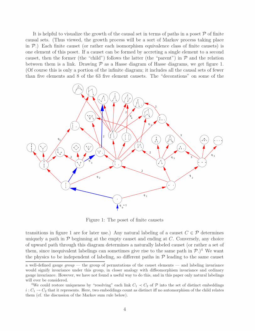
It is helpful to visualize the growth of the causal set in terms of paths in a poset P of finitecausal sets. (Thus viewed, the growth process will be a sort of Markov process taking placein P.) Each finite causet (or rather each isomorphism equivalence class of finite causets) isone element of this poset. If a causet can be formed by accreting a single element to a secondcauset, then the former (the “child”) follows the latter (the “parent”) in P and the relationbetween them is a link. Drawing P as a Hasse diagram of Hasse diagrams, we get figure 1.(Of course this is only a portion of the infinite diagram; it includes all the causal sets of fewerthan five elements and 8 of the 63 five element causets. The “decorations” on some of the

q 3

q = 10

2

2

3

3

q

q

q

q

qq

q

3

33

2

1

2

q4

2

2

2

23

Figure 1: The poset of finite causets

transitions in figure 1 are for later use.) Any natural labeling of a causet C ∈ P determinesuniquely a path in P beginning at the empty causet and ending at C. Conversely, any choiceof upward path through this diagram determines a naturally labeled causet (or rather a set ofthem, since inequivalent labelings can sometimes give rise to the same path in P.)4 We wantthe physics to be independent of labeling, so different paths in P leading to the same causet

a well-defined gauge group — the group of permutations of the causet elements — and labeling invariancewould signify invariance under this group, in closer analogy with diffeomorphism invariance and ordinarygauge invariance. However, we have not found a useful way to do this, and in this paper only natural labelingswill ever be considered.

4We could restore uniqueness by “resolving” each link C1 ≺ C2 of P into the set of distinct embeddingsi : C1 → C2 that it represents. Here, two embeddings count as distinct iff no automorphism of the child relatesthem (cf. the discussion of the Markov sum rule below).

4

should be regarded as representing the same (partial) universe, the distinction between thembeing “pure gauge”.

The causal sets which can be formed by adjoining a single maximal element to a givencauset will be called collectively a family. The causet from which they come is their parent,and they are siblings of each other. Each one is a child of the parent. The child formedby adjoining an element which is to the future of every element of the parent will be calledthe timid child. The child formed by adjoining an element which is spacelike to every otherelement will be called the gregarious child.

Each parent-child relationship in P describes a ‘transition’ C → C ′, from one causal set toanother induced by the birth of a new element. The past of the new element (a subset of C)will be referred to as the precursor set of the transition (or sometimes just the “precursor ofthe transition”). Normally, this precursor set is uniquely determined up to automorphism ofthe parent by the (isomorphism equivalence class of the) child, but (rather remarkably) thisis not always the case. The symbol Cn will denote the set of causets with n elements, and theset of all transitions from Cn to Cn+1 will be called stage n.

As just remarked, each parent-child transition corresponds to a choice of partial stem in theparent (the precursor of the transition). Since there is a one-to-one correspondence betweenpartial stems and antichains, a choice of child also corresponds to a choice of (possibly empty)antichain in the parent, the antichain in question being the set of maximal elements of thepast of the new element. Note also that the new element will be linked to each element ofthis antichain.

1.2 Some examples

To help clarify the terminology introduced in the previous section, we give some examples.The 20 element causet of figure 2 was generated by the stochastic dynamics described herein,with the choice of parameters given by equation (16) below. In the copy of this causet on theleft, the past of element a is highlighted. Notice that since we use the irreflexive conventionfor the order, a is not included in its own past. In the the copy on the right, a partial stem ofthe causet is highlighted.

Figure 3 shows rr r

r r

�� and its children. The timid child is Cb and the gregarious child is Cc.The precursor set leading to the transition to Cd is shown in the ellipse. An example of anautomorphism of Ca is the map a ↔ c, b ↔ d (the other elements remaining unchanged).

2 Transitive Percolation

In a sum over histories formulation of causal set theory, one might expect sums like

∑

C

A(C, {q}) (1)

to be involved, where A is a complex amplitude for the causal set C, possibly depending ona set of parameters {q}. Kleitman and Rothschild have shown that the number of posets ofcardinality n grows faster than exponentially in n and that asymptotically, almost every posethas a certain, almost trivial, “generic” form. (See [11].) Such a “generic poset” consists of three

5

Past of element ‘a’ A partial stem

a

Figure 2: An example of a (‘typical’?) 20 element causal set

gregariouschild

parent

siblings

child

timid child

precursorset

a c

C

C

C

C

C c

d

e

a

b

db

Figure 3: A family

6

“tiers”, with n/2 elements in the middle tier and n/4 elements in the top and bottom tiers.For this reason, one might think that a sum like (1) would be dominated by causets whichin no way resemble a spacetime, leading to a sort of “entropy catastrophe”. Nevertheless,it is not hard to forestall this catastrophe, and in fact the most naive choice of stochasticdynamics already does so. (Maybe this is not so different from the situation in ordinaryquantum mechanics, where the smooth paths, which form a set of measure zero in the spaceof all paths, are the ones which dominate the sum over histories in the classical limit.)

The dynamics in question, which we will call “transitive percolation”, is perhaps the mostobvious model of a randomly growing causet. It is an especially simple instance of a sequentialgrowth dynamics, in which each new element forges a causal bond independently with eachexisting element with probability p, where p ∈ [0, 1] is a fixed parameter of the model. (Anycausal relation implied by transitivity must then be added in as well.)

From a more static perspective, one can also describe transitive percolation by the followingalgorithm for generating a random poset:

1. Start with n elements labeled 0, 1, 2, · · · , n − 1 (n = ∞ is not excluded.)

2. With a fixed probability p, introduce a relation between every pair of points labeled iand j, where i < j.

3. Form the transitive closure of these relations (e.g. if 2 ≺ 5 and 5 ≺ 8 then enforce that2 ≺ 8.)

Expressed in this manner, the model appears as a species of one dimensional directed perco-lation; hence the name we have given it (following D. Meyer).

From a physical point of view, transitive percolation has some appealing features, both as amodel for a relatively small region of spacetime and as a cosmological model for spacetime as awhole. For p ∼ 1/n, there is a percolation transition, where the causet goes qualitatively froma large number of small disconnected universes for p < pcrit to a single connected universefor p > pcrit. Moreover, computer simulations suggest strongly that the model possesses acontinuum limit and exhibits scaling behavior in that limit with p scaling roughly like c log n/n[12, 13]. The “cosmology” of transitive percolation is also suggestive — the universe cyclesendlessly through phases of expansion, stasis, and contraction (via fluctuation) back down toa single element [14].

From all this, it is clear that the causets generated by transitive percolation do not atall resemble the 3-tier, generic causets of Kleitman and Rothschild, but rather they have thepotential to reproduce a spacetime or a part of one. Nevertheless, the dynamics of transitivepercolation is not viable as a theory of quantum gravity. One obvious reason is that it isstochastic only in the purely classical sense, lacking quantum interference. Another reason isthat the future of any element of the causet is completely independent of anything “spacelikerelated” to that element. Therefore, the only spacetimes which a causal set generated bytransitive percolation could hope to resemble would be homogeneous, such as the Minkowskior de Sitter spacetimes; but neither of these possibilities is compatible with the periodic re-collapses alluded to earlier. At best, therefore, one could hope to reproduce a small portionof such a homogeneous spacetime.

7

����������������������������������������������

����������������������������������������������

������������������

������������������

"post"

Figure 4: Transitive percolation cosmology

On the other hand, in computer simulations of transitive percolation [15], two independent(and coarse-graining invariant) dimension estimators have tended to agree with each other, onesuch estimator being that of [16] and the other being a simple “midpoint scaling dimension”.(Some other indicators of manifold-like behavior have tended to do much more poorly, butthose are not invariant under coarse graining, whereas one would in any case expect to observemanifold like behavior only for a sufficiently coarse grained causal set.) In the pure percolationmodel, however, these dimension indicators vary with time (i.e. with n) and one must rescalep if one wishes to hold the spacetime dimension constant. One may ask, then, if the modelcan be generalized by having p vary with n in an appropriate sense. We will see in the nextsection that something rather like this is in fact possible.

The transitive percolation model, incidentally, has attracted the interest of both mathe-maticians and physicists for reasons having nothing to do with quantum gravity. By physicists,it has been studied as a problem in the statistical mechanical field of percolation, as we havealready alluded to. By mathematicians, it has been studied extensively as a branch of randomgraph theory (a poset being the same thing as a transitive acyclic directed graph). Some ref-erences on transitive percolation (viewed from whatever angle) are [11, 14, 17, 18, 15, 12, 13].

3 Physical requirements on the dynamics

As discussed in the previous section, one can think of transitive percolation as a sort of“birth process”, but as such, it is only one special case drawn from a much larger universe ofpossibilities. As preparation for describing these more general possible dynamical rules, let usconsider the growth-sequence of a causal set universe.

First element ‘0’ appears (say with probability one, since the universe exists). Then element‘1’ appears, either related to ‘0’ or not. Then element ‘2’ appears, either related to ‘0’ or ‘1’,or both, or neither. Of course if 1 ≻ 0 and 2 ≻ 1 then 2 ≻ 0 by transitivity. Then element ‘3’appears with some consistent set of ancestors, and so on and so forth. Because of transitivity,each new element ends up with a partial stem of the previous causet as its precursor set. Theresult of this process, obviously, is a naturally labeled causet (finite if we stop at some finitestage, or infinite if we do not) whose labels record the order of succession of the individualbirths. For illustration, consider the path in figure 1 delineated by the heavy arrows. Along

8

this path, element ‘0’ appears initially, then element ‘1’ appears to the future of element‘0’, then element ‘2’ appears to the future of element ‘0’, but not to the future of ‘1’, thenelement ‘3’ appears unrelated to any existing element, then element ‘4’ appears to the futureof elements ‘0’, ‘1’ (say, or ‘2’, it doesn’t matter) and ‘3’, then element ‘5’ appears (not shownin the diagram), etc.

Let us emphasize once more that the labels 0, 1, 2, etc. are not supposed to be physicallysignificant. Rather, the “external time” that they record is just a way to conceptualize theprocess, and any two birth sequences related to each other by a permutation of their labelsare to be regarded as physically identical.

So far, we have been describing the kinematics of sequential growth. In order to define adynamics for it, we may give, for each n-element causet C, the transition probability from itto each of its possible children. Equivalently, we give a transition probability for each partialstem within C. We wish to construct a general theory for these transition probabilities bysubjecting them to certain natural conditions. In other words, we want to construct the mostgeneral (classically stochastic) “sequential growth dynamics” for causal sets.5 In stating thefollowing conditions, we will employ the terminology introduced in the Introduction.

The condition of internal temporality

By this imposing sounding phrase, we mean simply that each element is born either to thefuture of, or unrelated to, all existing elements; that is, no element can arise to the past of anexisting element.

We have already assumed this tacitly in describing what we mean by a sequential growthdynamics. An equivalent formulation is that the labeling induced by the order of birth mustbe natural, as defined above. The logic behind the requirement of internal temporality is thatall physical time is that of the intrinsic order defining the causal set itself. For an element tobe born to the past of another would be contradictory: it would mean that an event occurred“before” another which intrinsically preceded it.

The condition of discrete general covariance

As we have been emphasizing, the “external time” in which the causal set grows (equivalentlythe induced labeling of the resulting poset) is not meant to carry any physical information.We interpret this in the present context as being the condition that the net probability offorming any particular n-element causet C is independent of the order of birth we attribute toits elements. Thus, if γ is any path through the poset P of finite causal sets that originates atthe empty causet and terminates at C, then the product of the transition probabilities alongthe links of γ must be the same as for any other path arriving at C. (So general covariance inthis setting is a type of path independence). We should recall here, however, that, as observedearlier, a link in P can sometimes represent more than one possible transition. Thus ourstatement of path-independence, to be technically correct, should say that the answer is the

5By choosing to specify our stochastic process in terms of transition probabilities, we have assumed ineffect that the process is Markovian. Although this might seem to entail a loss of generality, the loss is onlyapparent, because the condition of discrete general covariance introduced below would have forced the Markovassumption on us, even if we had not already adopted it.

9

same no matter which transition (partial stem) we select to represent the link. Obviously, thisimmediately entails that all such representatives share the same transition probability.

We might with justice have required here conditions that are apparently much stronger,including the condition that any two paths through P with the same initial and final endpointshave the same product of transition probabilities. However, it is easy to see that this alreadyfollows from the condition stated.6 We therefore do not make it part of our definition ofdiscrete general covariance, although we will be using it crucially.

Finally, it is well to remark here that just because the “arrival probability at C” is inde-pendent of path/labeling, that does not necessarily mean that it carries an invariant meaning.On the contrary a statement like “when the causet had 8 elements it was a chain” is itselfmeaningless before a certain birth order is chosen. This, also, is an aspect of the gauge prob-lem, but not one that functions as a constraint on the transition probabilities that define ourdynamics. Rather it limits the physically meaningful questions that we can ask of the dynam-ics. Technically, we expect that our dynamics (like any stochastic process) can be interpretedas a probability measure on a certain σ-algebra, and the requirement of general covariancewill then serve to select the subalgebra of sets whose measures have direct physical meaning.

The Bell causality condition

The condition of “internal temporality” may be viewed as a very weak type of causalitycondition. The further causality condition we introduce now is quite strong, being similar tothat from which one derives Bell’s inequalities. We believe that such a condition is appropriatefor a classical theory, and we expect that some analog will be valid in the quantum case as well.(On the other hand, we would have to abandon Bell causality if our aim were to reproducequantum effects from a classical stochastic dynamics, as is sometimes advocated in the contextof “hidden variable theories”. Given the inherent non-locality of causal sets, there is no logicalreason why such an attempt would have to fail.)

The physical idea behind our condition is that events occurring in some part of a causalset C should be influenced only by the portion of C lying to their past. In this way, the orderrelation constituting C will be causal in the dynamical sense, and not only in name. In termsof our sequential growth dynamics, we make this precise as the requirement that the ratio ofthe transition probabilities leading to two possible children of a given causet depend only onthe triad consisting of the two corresponding precursor sets and their union.

Thus, let C → C1 designate a transition from C ∈ Cn to C1 ∈ Cn+1, and similarly forC → C2. Then, the Bell causality condition can be expressed as the equality of two ratios7:

prob(C → C1)

prob(C → C2)=

prob(B → B1)

prob(B → B2)(2)

where B ∈ Cm, m ≤ n, is the union of the precursor set of C → C1 with the precursor setof C → C2, B1 ∈ Cm+1 is B with an element added in the same manner as in the transition

6If γ does not start with the empty causet C0, but at Cs, we can extend it to start at C0 by choosing anyfixed path from C0 to Cs. Then different paths from Cs to Ce correspond to different paths between C0 andCe, and the equality of net probabilities for the latter implies the same thing for the former.

7In writing (2), we assume for simplicity that both numerators and both denominators are nonzero, thisbeing the only case we will have occasion to treat in the present paper.

10

C → C1, and B2 ∈ Cm+1 is B with an element added in the same manner as in the transitionC → C2.

8 (Notice that if the union of the precursor sets is the entire parent causet, then theBell causality condition reduces to a trivial identity.)

To clarify the relationships among the causets involved, it may help to characterize thelatter in yet another way. Let e1 be the element born in the transition C → C1 and let e2

be the element born in the transition C → C2. Then Ci = C ∪ {ei} (i = 1, 2), and we haveB = (past e1) ∪ (past e2) and Bi = B ∪ {ei} (i = 1, 2).

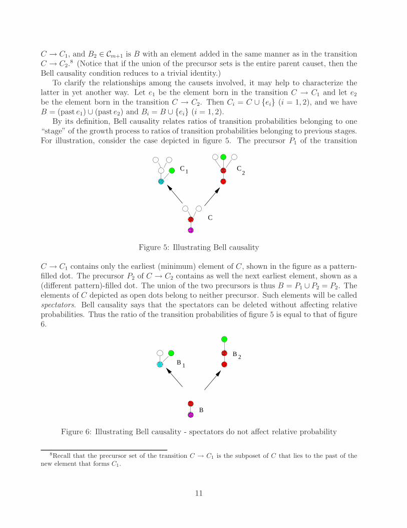
By its definition, Bell causality relates ratios of transition probabilities belonging to one“stage” of the growth process to ratios of transition probabilities belonging to previous stages.For illustration, consider the case depicted in figure 5. The precursor P1 of the transition

������

������

������

������

������

������

������

������

��������

C 1 C2

C

Figure 5: Illustrating Bell causality

C → C1 contains only the earliest (minimum) element of C, shown in the figure as a pattern-filled dot. The precursor P2 of C → C2 contains as well the next earliest element, shown as a(different pattern)-filled dot. The union of the two precursors is thus B = P1 ∪ P2 = P2. Theelements of C depicted as open dots belong to neither precursor. Such elements will be calledspectators. Bell causality says that the spectators can be deleted without affecting relativeprobabilities. Thus the ratio of the transition probabilities of figure 5 is equal to that of figure6.

���

���

���

���

����

��������

������

������ B

B 1

B 2

Figure 6: Illustrating Bell causality - spectators do not affect relative probability

8Recall that the precursor set of the transition C → C1 is the subposet of C that lies to the past of thenew element that forms C1.

11

The Markov sum rule

As with any Markov process, we must require that the sum of the full set of transition prob-abilities issuing from a given causet be unity. However, the set we have to sum over dependsin a subtle manner on the extent to which we regard causal set elements as “distinguishable”.Heretofore we have identified distinct transitions with distinct precursor sets of the parent. Indoing so, we have in effect been treating causet elements as distinguishable (by not identifyingwith each other, precursor sets related by automorphisms of the parent), and this is what weshall continue to do. Indeed, this is the counting of children used implicitly by transitivepercolation, so we keep it here for consistency. With respect to the diagram of figure 1, thismethod of counting has the effect of introducing coefficients into the sum rule, equal to thenumber of partial stems of the parent which could be the precursor set of the transition.For the transitions depicted there, these coefficients (when not one) are shown next to thecorresponding arrow.9

We remark here that these sum-rule coefficients admit an alternative description in termsof embeddings of the parent into the child (as a partial stem). Instead of saying “the numberof partial stems of the parent which could be the past of the new element”, we could say “thenumber of order preserving injective maps from the parent onto partial stems of the child,divided by the number of automorphisms of the child”. (The proof of this equivalence willappear in [19].)

4 The general form of the transition probabilities

We seek to derive a general prescription which gives, consistent with our requirements, thetransition probability from an element of Cn to an element of Cn+1. To avoid having to dealwith special cases, we will assume throughout that no transition probability vanishes. Thusthe solution we find may be termed “generic”, but not absolutely general.

In this connection, we want to point out that one probably does not obtain every possiblesolution of our conditions by taking limits of the generic solution, and the special theories whichresult from taking certain transition probabilities to vanish must be treated separately.10 Onesuch special theory is the originary percolation model, which is the same as the transitivepercolation model, but with the added restriction that each element except the original onemust have at least one ancestor among the previous elements. The net effect is that thegrowing causal set is required to have an “origin” (= unique minimum element) at all stages.(Generalizations are also possible in which a more complex full stem of the causet is enforced.)The poset of originary causets can be transformed into the poset of all causets (exactly) byremoving the origin from every originary causet. The transition probabilities for originarypercolation are just those of ordinary transitive percolation with an added factor of (1 − qn)

9One might describe the result of setting these coefficients to unity as the case of “indistinguishable causetelements”. It appears that in this case a dynamics with a richer structure obtains: instead of the transitionprobability depending only on the size of the precursor set and the number of its maximal elements, it issensitive to more details of the precursor set’s structure.

10Indeed, the requirement of Bell causality itself must be given an unambiguous interpretation when someof the transition probabilities involved are zero.

12

in the denominator at stage n.

4.1 Counting the free parameters

A theory of the sort we are seeking provides a probability for each transition, so without furtherrestriction, it would contain a free parameter for every possible antichain of every possible(finite) causet. We will see, however, that the requirements described above in Section 3drastically limit this freedom.

Lemma 1 There is at most one free parameter per family.

Proof: Consider a parent and its children. Every such child, except the timid child, partici-pates in a Bell causality equation with the gregarious child. (See the proof of Lemma 5 in theAppendix.) Hence (since Bell causality equates ratios), all these transitions are determinedup to an overall factor. This leaves two free parameters for the family. The Markov sum rulegives another equation, which exhausts itself in determining the probability of the timid child.Hence precisely one free parameter per family remains after Bell Causality and the sum ruleare imposed. 2

Lemma 2 The probability to add a completely disconnected element (the “gregarious childtransition”) depends only on the cardinality of the parent causal set.

Proof: Consider an arbitrary causet A, with a maximal element e, as indicated in figure 7.

����������������

����������������

����������������

����������������

����������������

����������������

����������������

����������������

��������������������

��������������������

��������������������

��������������������

��������������������

��������������������

��������������������

��������������������

x

a b

w

D

BE

A

e

ef

f

f

f

f

C

G

y z

F etc

Figure 7: Equality of “gregarious child” transitions

Adjoining a disconnected element to A produces the causet B. Then, removing e from B leadsto the causet C, which can be looked upon as the gregarious child of the causet D = A\{e}.Adding another disconnected element to C leads to a causet E with (at least) two completelydisconnected elements. Now, by general covariance,

ax = bw

13

and by Bell causality,y

w=

b

a

(the disconnected element in C acts as the spectator here). Thus

ax = bw = ay =⇒ x = y

(Recall that we have assumed that no transition probability vanishes.) Repeating our deduc-tions with C in the place of A in the above argument (and a new maximal element f in theplace of e), we see that y = z, where z is the probability for the transition from F to G asshown. Continuing in this way until we reach the antichain An shows finally that x = qn,where we define qn as the transition probability from the n-antichain to the (n+1)-antichain.Since our starting causet A was not chosen specially, this completes the proof. 2

If our causal sets are regarded as entire universes, then a gregarious child transition corre-sponds to the spawning of a new, completely disconnected universe (which is not to say thatthis new universe will not connect up with the existing universe in the future). Lemma 2proves that the probability for this to occur does not depend on the internal structure of theexisting universe, but only on its size, which seems eminently reasonable. In the sequel, wewill call this probability qn.

With Lemmas 1 and 2, we have reduced the number of free parameters (since every familyhas a gregarious child) to 1 per stage, or what is the same thing, to one per causal setelement. In the next sections we will see that no further reduction is possible based on ourstated conditions. Thus, the transition probabilities qn can be identified as the free parametersor “coupling constants” of the theory. They are, however, restricted further by inequalitiesthat we will derive below.

4.2 The general transition probability in closed form

Given the qn, the remaining transition probabilities (for the non-gregarious children) aredetermined by Bell causality and the sum rule, as we have seen. Here we derive an expressionin closed form for an arbitrary transition probability in terms of causet invariants and theparameters qn.

Mathematical form of transition probabilities

We use the following notation:

αn an arbitrary transition probability from Cn to Cn+1

βn a transition whose precursor set is not the entire parent (‘non-timid’ transition)γn a transition whose precursor set is the entire parent (‘timid’ transition)

Notice that the subscript n here refers only to the number of elements of the parent causet; itdoes not exhibit which particular transition of stage n is intended. A more complete notationmight provide α, β and γ with further indices to specify both the parent causet and theprecursor set within the parent.

We also set q0 ≡ 1 by convention.

14

Lemma 3 Each transition probability αn of stage n has the form

qn

n∑

i=0

λi

1

qi

(3)

where the λi are integers depending on the individual transition in question.

Proof: This is easily seen to be true for stages 0 and 1. Assume it is true for stage n − 1.Consider a non-timid transition probability βn of stage n. Bell causality gives

βn

qn

=αn−1

qn−1

where αn−1 is an appropriate transition probability from stage n − 1. So by induction

βn = αn−1qn

qn−1

=n−1∑

i=0

λi

qn−1

qi

qn

qn−1

=n−1∑

i=0

λi

qn

qi

. (4)

For a timid transition probability γn, we use the Markov sum rule:

γn = 1 −∑

j

βnj (5)

where j labels the possible non-timid transitions (i.e. the set of proper partial stems of theparent).11 But then, substituting (4) yields immediately

γn = 1 −∑

j

n−1∑

i=0

λji

qi

qn = 1 −n−1∑

i=0

∑j λji

qi

qn ,

which we clearly can put into the form (3) by taking λi = −∑

j λji for i < n and λn = 1. 2

Another look at transitive percolation

The transitive percolation model we described earlier is consistent with the four conditions ofSection 3. To see this, consider an arbitrary causal set Cn of size n. The transition probabilityαn from Cn to a specified causet Cn+1 of size n + 1 is given by

αn = pm(1 − p)n− (6)

where m is the number of maximal elements in the precursor set and is the size of the entireprecursor set. (This becomes clear if one recalls how the precursor set of a newborn elementis generated in transitive percolation: first a set of ancestors is selected at random, and thenthe ancestors implied by transitivity are added. From this, it follows immediately that a givenstem S ⊆ Cn results from the procedure iff (i) every maximal element of S is selected in thefirst step, and (ii) no element of Cn\S is selected in the first step.) In particular, we see thatthe “gregarious transition” will occur with probability qn = qn, where q = 1 − p.

11Of course, more than one stem will in general correspond to the same link in P . If we redefined j to runover links in P , then (5) would read γn = 1 −

∑j χjβnj , where χj is the “multiplicity” of the jth link.

15

Now consider our four conditions. Internal temporality was built in from the outset, as weknow. Discrete general covariance is seen to hold upon writing the net probability of a givenCn explicitly in terms of causet invariants (writing it in “manifestly covariant form”) as

P (Cn) = WpLq(n

2)−R

where L is the number of links in Cn, R the number of relations, and W the number of(natural) labelings of Cn.

To see that transitive percolation obeys Bell causality, consider an arbitrary parent causet.The transition probability to a given child is exhibited in eq. (6). Consider two different chil-dren, one with (m, )=(m1,1) and the other with (m, )=(m2,2). Bell causality requiresthat the ratio of their transition probabilities be the same as if the parent were reduced tothe union of the precursor sets of the two transitions, i.e. it requires

pm1qn−1

pm2qn−2

=pm1qn′−1

pm2qn′−2

where n′ is the cardinality of the union of the precursor sets of the two transitions. Thus, Bellcausality is satisfied by inspection.

Finally, the Markov sum rule is essentially trivial. At each stage of the growth process,a preliminary choice of ancestors is made by a well-defined probabilistic procedure, and eachsuch choice is mapped uniquely onto a choice of partial stem. Thus the induced probabilitiesof the partial stems sum automatically to unity.

The general transition probability

In the previous section we have shown that transitive percolation produces transition proba-bilities (6) consistent with all our conditions. By equating the right hand side of (6) to thegeneral form (3) of Lemma 3, we can solve for the λi and thus obtain the general solution ofour conditions:

αn =n∑

i=0

λi

1

qi

qn = pm(1 − p)n− = (1 − q)mqn−

Expanding the factor (1 − q)m, and using the fact that qn = qn for transitive percolation, weget

λi = (−)−i

(m

− i

).

So an arbitrary transition probability in the general dynamics is, according to (3)

αn =n∑

i=0

(−)−i

(m

− i

)qn

qi

.

Noting that the binomial coefficients are zero for − i /∈ {0..m}, and rearranging the indices,we obtain

αn =m∑

k=0

(−)k

(m

k

)qn

q−k

. (7)

16

This form for the transition probability exhibits its causal nature particularly clearly: ex-cept for the overall normalization factor qn, αn depends only on invariants of the associatedprecursor set.

4.3 Inequalities

Since the αn are classical probabilities, each must lie between 0 and 1, and this in turn restrictsthe possible values of the qn. Here we show that it suffices to impose only one inequality perstage; all the others (two per child) then follow. More precisely, what we show is that, ifqn > 0 for all n, and if αn ≥ 0 for the “timid” transition from the n-antichain, then all the αn

lie in [0, 1]. This we establish in the following two “Claims”.

Claim In order that all the transition probabilities αn fall between 0 and 1, it suffices thateach timid transition probability be ≥ 0.

Proof: As described in the proofs of lemmas 1 and 5, each non-timid transition (of stage n)is given (via Bell causality) by

αn = αm

qn

qm

where m is some natural number less than n. The q’s are positive. So if the probabilities ofthe previous stages are positive, then the non-timid probabilities of stage n are also positive.It follows by induction that all but the timid transition probabilities are positive (since α0 =q0 = 1 obviously is). But for the timid transition of each family, we have

γn = 1 −∑

i

βi (8)

where each βi is positive. If any of the βi is greater than one, γn will obviously be negative.Also (8) plainly cannot be greater than one. Consequently, if we require that γn be positive,then all transition probabilities in the family will be in [0, 1]. 2

In a timid transition, the entire parent is the precursor set, so = n. The inequalitiesconstraining each probability of a given family to be in [0, 1] therefore reduce to the solecondition

m∑

k=0

(−)k

(m

k

)1

qn−k

≥ 0 . (9)

Claim The most restrictive inequality of stage n is the one arising from the n-antichain, i.e.the one for which m = n. All other inequalities of stage n follow from this inequality and theinequalities for smaller n.

Proof: Assume that we have, for m = n,n∑

k=0

(−)k

(n

k

)1

qn−k

≥ 0.

Add to this the inequality from stage n − 1,

n−1∑

k=0

(−)k

(n − 1

k

)1

qn−k−1

=n∑

k=0

(−)k−1

(n − 1

k − 1

)1

qn−k

≥ 0

17

to getn−1∑

k=0

(−)k

(n − 1

k

)1

qn−k

≥ 0.

This is the inequality of stage n for m = n−1. (We have used the identity(

n

k

)=(

n−1k

)+(

n−1k−1

).)

Adding to it the inequality of stage n − 1 with m = n − 2 yields the inequality of stage n form = n − 2. Repeating this process will give all the inequalities of stage n. 2

It is helpful to introduce the quantities

tn =n∑

k=0

(−)n−k

(n

k

)1

qk

(10)

Obviously, we have t0 = 1 (since q0 = 1), and we have seen that the full set of inequalitiesrestricting the qn will be satisfied iff tn ≥ 0 for all n. (Recall we are assuming qn > 0, ∀n.)Moreover, given the tn, we can recover the qn by inverting (10):

Lemma 41

qn

=n∑

k=0

(n

k

)tk (11)

Proof: This follows immediately from the identity

n∑

k=0

(n

k

)(−)n−k

(k

m

)= δn

m 2

Thus, the tn may be treated as free parameters (subject only to tn ≥ 0 and t0 = 1), and theqn can then be derived from (11). If this is done, the remaining transition probabilities αn

can be re-expressed more simply in terms of the tn by inserting (11) into (7) to get

αn

qn

=∑

l

tl∑

k

(−)k

(m

k

)( − k

l

)=∑

l

tl

( − m

− l

)

whence

αn =

∑l=m

(−m

−l

)tl

∑nj=0

(n

j

)tj

(12)

Here, we have used an identity for binomial coefficients that can be found on page 63 of [20].In this way, we arrive at the general solution of our inequalities. (Actually, we go slightly

beyond our “genericity” assumption that αn 6= 0 if we allow some of the tn to vanish; but noharm is done thereby.)

Let us conclude this section by noting that (11) implies

q0 ≡ 1 ≥ q1 ≥ q2 ≥ q3 ≥ · · · (13)

If we think of the qn as the basic parameters or “coupling constants” of our sequential growthdynamics, then it is as if the universe had a free choice of one parameter at each stage of the

18

process. We thus get an “evolving dynamical law”, but the evolution is not absolutely free,since the allowable values of qn at every stage are limited by the choices already made. On theother hand, if we think of the tn as the basic parameters, then the free choice is unencumberedat each stage. However, unlike the qn, the tn cannot be identified with any dynamical transitionprobability. Rather, they can be realized as ratios of two such probabilities, namely as theratio xn/qn, where xn is the transition probability from an antichain of n elements to thetimid child of that antichain. (Thus, if we suppose that the evolving causet at the beginningof stage n is an antichain, then tn is the probability that the next element will be born to thefuture of every element, divided by the probability that the next element will be born to thefuture of no element.)

4.4 Proof that this dynamics obeys the physical requirements

To complete our derivation, we must show that the sequential growth dynamics given by (7)or (12) obeys the four conditions set out in section 3.

Internal temporality

This condition is built into our definition of the growth process.

Discrete general covariance

We have to show that the product of the transition probabilities αn associated with a labelingof a fixed finite causet C is independent of the labeling. But this follows immediately from(7) [or (12)] once we notice that what remains after the overall product

|C|−1∏

j=0

qj

is factored out, is a product over all elements x ∈ C of poset invariants depending only on thestructure of past(x).

Bell causality

Bell causality states that the ratio of the transition probabilities for two siblings depends onlyon the union of their precursors. Looking at (7), consider the ratio of two such probabilitiesαn1 and αn2. The qn factors will cancel, leading to an expression which depends only on 1,2, m1, and m2. Since these are all determined by the structure of the precursor sets, Bellcausality is satisfied.

Markov sum rule

The sum rule states that the sum of all transition probabilities αn from a given parent C (ofcardinality |C| = n) is unity. Since a child can be identified with a partial stem of the parent,

19

we can write this condition, in view of (12), as

∑

S

∑

l

tl

(|S| − m(S)

l − m(S)

)=∑

j

tj

(n

j

)(14)

where S ranges over the partial stems of C. This must hold for any tl, since they may bechosen freely. Reordering the sums and equating like terms yields

∀l,∑

S

(|S| − m(S)

l − m(S)

)=

(n

l

), (15)

an infinite set of identities which must hold if the sum rule is to be satisfied by our dynamics.The simplest way to see that (15) is true is to resort to transitive percolation, for which

tl = tl, where t = p/q = p/(1 − p). In that case we know that the sum rule is satisfied, so byinspection of (14), we see that the identity (15) must be true.

A more intuitive proof is illustrated well by the case of l = 3. Group the terms on the leftside according to the number of maximal elements:

∑S |m(S)=0

(|S|−03−0

)+

∑S |m(S)=1

(|S|−13−1

)+

∑S |m(S)=2

(|S|−23−2

)+

∑S |m(S)=3

(|S|−33−3

)=

(n

3

)

0 +∑

S |m(S)=1

(|S|−1

2

)+

∑S |m(S)=2

(|S| − 2) +∑

S |m(S)=31 =

(n

3

)

The first term is zero because the only partial stem with zero maximal elements is empty (i.e.|S| = 0). The second term is a sum over all partial stems with one maximal element. This isequivalent to a sum over elements, with the element’s inclusive past forming the partial stem.The summand chooses every possible pair of elements to the past of the maximal element.Thus the second term overall counts the 3-element subcausets of C with a single maximalelement. There are two possibilities here, the three-chain r

r

r

and the “lambda”r

r r��AA . The thirdterm sums over partial stems with two maximal elements, which is equivalent to summing over2 element antichains, the inclusive past of the antichain being the partial stem. The summandthen counts the number of elements to the past of the two maximal ones. Thus the third termoverall counts the number of three element subcausets with precisely two maximal elements.Again there are two possibilities, the “V” r

r r

AA�� , and the “L”, r r

r

. Finally, the fourth term isa sum over partial stems with three maximal elements, and this can be interpreted as a sumover all three element antichains r r r. As this example illustrates, then, the left hand side of(15) counts the number of l element subcausets of C, placing them into “bins” according tothe number of maximal elements of the subcauset. Adding together the bin sizes yields thetotal number of l element subsets of C, which of course equals

(n

l

).

4.5 Sample cosmologies

The physical consequences of differing choices of the tn remain to be explored. To get aninitial feel for this question, we list some simple examples. (Recall our convention that t0 = 1,or equivalently, q0 = 1, where q0 is the probability that the universe is born at all.12)

12So, is the answer to the old question why something exists rather than nothing, simply that it is nota-tionally more convenient for it to be so?

20

• “Dust universe”t0 = 1, ti = 0, i ≥ 1

This universe is simply an antichain, since, according to (11), qn = 1 for all n.

• “Forest universe”t0 = t1 = 1; ti = 0, i ≥ 2

This yields a universe consisting wholly of trees, since (see the next example) t2 = t3 =t4 = · · · = 0 implies that no element of the causet can have more than one past link.The particular choice of t1 = 1 has in addition the remarkable property that, as followseasily from (12), every allowed transition of stage n has the same probability 1/(n + 1).

• Case of limited number of past links

ti = 0, i > n0

Referring to expression (12) one sees at once that αn vanishes if m > n0. Hence, noelement can be born with more than n0 past links or “parents”. This means in particularthat any realistic choice of parameters will have tn > 0 for all n, since an element of acausal set faithfully embeddable in Minkowski space would have an infinite number ofpast links.

• Transitive percolationtn = tn

We have seen that for transitive percolation, qn = qn, where q = 1 − p. Using thebinomial theorem, it is easy to learn from (11) or (10) that this choice of qn correspondsto tn = tn with t = p/q. Clearly, t runs from 0 to ∞ as p runs from 0 to 1.

• A more lifelike choice?

tn =1

n!(16)

We have seen that transitive percolation with constant p yields causets which couldreproduce — at best — only limited portions of Minkowski space. To do any better, onewould have to scale p so that it decreased with increasing n [12, 13, 15]. This suggeststhat tn should fall off faster than in any percolation model, hence (by the last example)faster than exponentially in n. Obviously, there are many possibilities of this sort (e.g.tn ∼ e−αn2

), but one of the simplest is tn ∼ c/n! This would be our candidate of themoment for a physically most realistic choice of parameters.

5 The stochastic growth process as such

We have seen that, associated with every labeled causet C of size N , is a net “probabilityof formation” P (C) which is the product of the transition probabilities αi of the individualbirths described by the labeling:

P (C) =N−1∏

i=0

αi

21

where αi = α(i, i, mi) is given by (7) or (12). We have also seen that P is in fact independentof the labeling and may be written as P (C) where C is the unlabeled causet correspondingto C. To bring this out more clearly, let us define

λ(, m) =∑

k=m

( − m

− k

)tk (17)

Then qi = λ(i, 0)−1 and we have

αi(i, i, mi) =λ(i, mi)

λ(i, 0),

whence P (C) =N−1∏i=0

λ(i, mi)/N−1∏j=0

λ(j, 0), or expressed more intrinsically,

P (C) =

∏x∈C

λ((x), m(x))

|C|−1∏j=0

λ(j, 0)

, (18)

where (x) = |pastx| and m(x) = |maximal(pastx)|. This expression, as far as it goes, ismanifestly “causal” and “covariant” in the senses explained above. As also explained above,however, it has no direct physical meaning. Here we briefly discuss some probabilities whichdo have a fully covariant meaning and show how, in simple cases, they are related to N → ∞limits of probabilities like (18).

First, let us notice that the net probability of arriving at a particular C ∈ P is not P (C)but

ProbN(C) = W (C) P (C)

where N = |C| and W (C) is the number of inequivalent13 labelings of C, or in other words,the total number of paths through P that arrive at C, each link being taken with its propermultiplicity.

Now as a rudimentary example of a truly covariant question, let us take “Does the two-chain ever occur as a partial stem of C?”. The answer to this question will be a probability,P , which it is natural to identify as

P = limN→∞

ProbN (XN) ,

where XN is the event that “at stage N”, C possesses a partial stem which is a two-chain. Inthis connection, we conjecture that the questions of the form “Does P occur as a partial stemof C?” furnish a physically complete set, when P ranges over all (isomorphism equivalenceclasses of) finite causets.

13Two labelings of C are equivalent iff related by an automorphism of C.

22

6 Two Ising-like state-models

In this section, we present two Ising-like state-models from which P (C) of equation (18) canbe obtained. In the main we just indicate the results, leaving the details to appear elsewhere[19]. The two models come from taking (7) or, respectively, (12) as the starting point. Ineach case, the idea is to interpret the binomial coefficients which occur in these formulas asdescribing a sum over subsets of relations of C. If we work with (7) these will be subsets ofthe set of links of C; if we work with (12) they will be subsets of the set of relations of C thatare not links.

Let us take first equation (7). Reinterpreting the binomial coefficients in the mannerindicated, and proceeding as in the derivation of (18), we arrive at an expression for P (C)in terms of a sum over Z2-valued “spins” σ living on the relations of C. In summing overconfigurations, however, the spins σ on the non-link relations are set permanently to 1; onlythose on the links vary. With σ = 1 interpreted as “presence” and σ = 0 as “absence”, thecontribution of a particular spin configuration σ is an overall sign times the product of one“vertex factor” for each x ∈ C. The vertex factor is q−1

r , where r is the number of presentrelations having x as future endpoint, and the sign is (−)a, where a is the number of absent

relations. (In addition, there is a constant overall factor in P (C) of∏|C|−1

j=0 qj .)In the second state model, we begin with (12), or better (18) itself, and proceed similarly.

The result is again a sum over spins σ residing on the relations, this time with all the termsbeing positive (as is required of physical Boltzmann weights). In this second model, the spinson the links are set permanently to 1 while those on the non-links vary. The “vertex factor”coming from x ∈ C now is tr, where r is again the number of relations present and “pointingto x”.

These two models (and especially the second) show that our sequential growth dynamicscan be viewed as a form of “induced gravity” obtained by summing over (“integrating out”)the values of our underlying spin variables σ. This underlying “matter” theory may or maynot be physically reasonable (Does it obey its own version of Bell causality, for example? Isit local in an appropriate sense?), but at a minimum, it serves to illustrate how a theory ofnon-gravitational matter can be hidden within a theory that one might think to be limited togravity alone.14 15

14In this connection, it bears remembering that Ising matter can produce fermionic as well as bosonic fields,at least in certain circumstances. [21, 22]

15References [23] and [24] (for which we thank an anonymous referee) describe a similar example of “hidden”matter fields in the context of 2-dimensional random surfaces (Euclidean signature quantum gravity) and theassociated matrix models in the continuum limit. Unfortunately, the matter fields used (Ising spins or “harddimers”) were unphysical in the sense that the partition function was a sum of Boltzmann weights which werenot in general real and positive. This is much like our first state model described above. To the extent that theanalogy between these two, rather different, situations holds good, our results here suggest that there mightbe, in addition to the matter fields employed in [24], another set of fields with physical choices of the couplingconstants, which could reproduce the same effective dynamics for the random surface.

23

7 Further Work

Our dynamics can be simulated; for tn = 1/n! it takes a minute or so to generate a 64 elementcauset on a DEC Alpha 600 workstation. Analytic results, so far, are available only for thespecial case of transitive percolation. An important question, of course, is whether some choiceof the tn can reproduce general relativity, or at least reproduce a Lorentzian manifold for somerange of t’s and of n = |C|. Similarly, one can ask whether our “Ising matter” gives rise toan interesting effective field theory and what relation it has with the local scalar matter on abackground causal set studied in [25, 26]?

Another set of questions concerns the possibility of a more “manifestly covariant” formu-lation of our sequential growth dynamics – or of more general forms of causal set dynamics.Can Bell causality be formulated in a gauge invariant manner, without reference to a choiceof birth sequence? Is our conjecture correct that all meaningful assertions are logical com-binations of assertions about the occurrence of partial stems (“past sets”)? (Such questionsseem likely to arise with special urgency in any attempt to generalize our dynamics to thequantum case.)

Also, there are the special cases we left unstudied. There exist originary analogs of all ofour dynamics, for example. Are there other special, non-generic cases of interest?

We might continue multiplying questions, but let’s finish with the question of how todiscover a quantum generalization of our dynamics. Since our theory is formulated as a typeof Markov process, and since a Markov process mathematically is a probability measure ona suitable sample space, the natural quantum generalization would seem to be a quantummeasure[1] (or equivalent “decoherence functional”) on the same sample space. The questionthen would be whether one could find appropriate quantum analogs of Bell causality andgeneral covariance formulated in terms of such a quantum measure. If so, we could hope that,just as in the classical case treated herein, these two principles would lead us to a relativelyunique quantum causet dynamics,16 or rather to a family of them among which a potentialquantum theory of gravity would be recognizable.

It is a pleasure to thank Avner Ash for a stimulating discussion at a critical stage of ourwork. The research reported here was supported in part by NSF grant PHY-9600620 and bya grant from the Office of Research and Computing of Syracuse University.

Appendix: Consistency of the conditions

Our analysis of the conditions of Bell causality et al. unfolded in the form of several lemmas.Here we present some similar lemmas which strictly speaking are not needed in the presentcontext, but which further elucidate the relationships among our conditions. We expect theselemmas can be useful in any attempt to formulate generalizations of our scheme, in particularquantal generalizations.

Lemma 5 The Bell causality equations are mutually consistent.

16See [27] for a promising first step toward such a dynamics.

24

����������������

����������������

��������

������������

����������������

������

������

��������������������

��������������������

��������������������

��������������������

������

������

�������������������������

���������������������������������

��������������������

��������������������

������

������

r r

r

2

ss

s1 3

2

1

3

C n

union of precursors

Figure 8: two families related by Bell causality

Proof: The top of figure 8 shows three children of an arbitrary causal set Cn. The shadedellipses represent portions of Cn. The small square indicates the new element whose birthtransforms Cn into a causal set Cn+1 of the next stage. The smaller ellipse “stacked on topof” the larger ellipse represents a subcauset of Cn which does not intersect the precursor setof any of the transitions being considered (i.e. none of its elements lie to the past of any ofthe new elements). This small ellipse thus consists entirely of “spectators” to the transitionsunder consideration. The bottom part of figure 8 shows the corresponding parent and childrenwhen these spectators are removed.

Notice that one of the three children is the gregarious child. We will show that theBell causality equations between this child and each of the others imply all remaining Bellcausality equations within this family. Since no Bell causality equation reaches outside a singlefamily (and since, within a family, the Bell causality equations that involve the gregariouschild obviously always possess a solution — in fact they determine all ratios of transitionprobabilities except for that to the timid child), this will prove the lemma.

In the figure t1 and t2 represent a general pair of transitions related by a Bell causalityequation, namely

t1t2

=s1

s2. (19)

But, as illustrated, each of these is also related by a Bell causality equation to the gregariouschild, to wit:

t1t3

=s1

s3and

t2t3

=s2

s3(20)

Since (19) follows immediately from (20), no inconsistencies can arise at stage n, and thelemma follows by induction on n. 2

Lemma 6 Given Bell causality and the further consequences of general covariance that are

25

embodied in Lemma 2, all the remaining general covariance equations reduce to identities, i.e.they place no further restriction on the parameters of the theory.

Proof: Discrete general covariance states that the probability of forming a causet is indepen-

����������������

����������������

��������������������

��������������������

��������������������

��������������������

��������������������

��������������������

��������������������

��������������������

��������������������

��������������������

��������������������

��������������������

D

B

A C

a

xz

b

q n

q

q n

n-1

Figure 9: consistency of remaining general covariance conditions

dent of the order in which the elements arise, i.e. it is independent of the corresponding paththrough the poset of finite causets.

Now, general covariance relations always can be taken to come from ‘diamonds’ in theposet of causets, for the following reason. As illustrated in figure 9, any two parents A, C ofa causet B will have a common parent D (a “grandparent” of B) obtained by removing twosuitable elements from B. (By assumption B must contain an element whose removal yields Aand another element whose removal yields C. Then remove these two elements. For example,consider the case where

r

rr r��AA is the grandchild and it has the parent r r r (by removing themaximal element of the wedge) and the parent

r

r r��AA (by removing the disconnected element).To find the grandparent r r remove both maximal elements from

r

rr r��AA .)Now, still referring to figure 9, let |D| = n and suppose inductively that all the general

covariance relations are satisfied up through stage n. A new condition arising at stage n + 1says that some path arriving at B via x has the same probability as some other path arrivingvia z. But, by our inductive assumption, each of these paths can be modified to go throughD without affecting its probability. Thus, the equality of our two path probabilities reducessimply to ax = bz.

Now by Bell causality and lemma 2,

x

qn

=b

qn−1,

whenceax = ab

qn

qn−1

.

But by symmetry, we also have

bz = baqn

qn−1;

therefore ax = bz, as required. 2

26

References

[1] Rafael D. Sorkin. Quantum mechanics as quantum measure theory. Modern PhysicsLetters A, 9(33):3119–3127, 1994. <e-print archive: gr-qc/9401003>.

[2] J.L. Friedman and A. Higuchi. State vectors in higher-dimensional gravity with quantumnumbers of quarks and leptons. Nuclear Physics B, 339:491–515, 1990.

[3] Rafael D. Sorkin. Forks in the road, on the way to quantum gravity. Int. J. Th. Phys.,36:2759–2781, 1997. talk given at the conference entitled “Directions in General Relativ-ity”, held at College Park, Maryland, May, 1993. <e-print archive: gr-qc/9706002>.

[4] Rafael D. Sorkin. Spacetime and causal sets. In J. C. D’Olivo, E. Nahmad-Achar,M. Rosenbaum, M.P. Ryan, L.F. Urrutia, and F. Zertuche, editors, Relativity and Grav-itation: Classical and Quantum, pages 150–173, Singapore, December 1991. World Sci-entific. (Proceedings of the SILARG VII Conference, held Cocoyoc, Mexico, December,1990).

[5] Luca Bombelli, Joohan Lee, David Meyer, and Rafael D. Sorkin. Space-time as a causalset. Physical Review Letters, 59:521–524, 1987.

[6] David Reid. Introduction to causal sets: an alternative view of spacetime structure.preprint, 1999.

[7] Luca Bombelli. Spacetime as a Causal Set. PhD thesis, Syracuse University, December1987.

[8] F. Markopoulou and L. Smolin, “Causal evolution of spin networks”, Nuc. Phys. B508:409-430 (1997) 〈e-print archive: gr-qc/9702025〉

[9] J. Ambjørn and R. Loll, “Non-perturbative Lorentzian quantum gravity, causality andtopology change”, Nuc. Phys. B 536: 407-434 (1999) 〈e-print archive: hep-th/9805108〉

[10] J. Ambjørn, K.N. Anagnostopoulos and R. Loll, “A New Perspective on Matter Couplingin 2d Quantum Gravity”, 〈e-print archive: hep-th/9904012〉

[11] Graham Brightwell. Models of random partial orders. In Keele, editor, Surveys in com-binatorics, volume 187 of London Math. Soc. Lecture Note Ser., pages 53–83. CambridgeUniversity Press, Cambridge, 1993.

[12] David P. Rideout and Rafael D. Sorkin. Continuum limit of percolated causal sets. (inpreparation).

[13] David P. Rideout and Rafael D. Sorkin. Scaling behavior of percolated causal sets. (inpreparation).

[14] Bela Bollobas and Graham Brightwell. The structure of random graph orders. Siam J.Discrete Math, 10(2):318–335, May 1997.

27

[15] Alan Daughton, Rafael D. Sorkin, and C.R. Stephens. Percolation and causal sets: A toymodel of quantum gravity. (in preparation).

[16] David A. Meyer. The Dimension of Causal Sets. PhD thesis, Massachusetts Institute ofTechnology, 1988.

[17] Bela Bollobas and Graham Brightwell. Graphs whose every transitive orientation containsalmost every relation. Israel Journal of Mathematics, 59(1):112–128, 1987.

[18] C. M. Newman and L. S. Schulman. One-dimensional 1/|j − i|s percolation models: theexistence of a transition for s ≤ 2. Comm. Math. Phys., 104(4):547–571, 1986.

[19] David P. Rideout. Causal Set Dynamics. PhD thesis, Syracuse University, 1999. (inpreparation).

[20] William Feller. An Introduction to Probability Theory and Its Applications, volume I.Wiley, 1957.

[21] Claude Itzykson and Jean-Michel Drouffe. Statistical Field Theory, volume 2. CambridgeUniversity Press, 1989.

[22] V. N. Plechko. Anticommuting integrals and fermionic field theories for two-dimensionalIsing models. August 1997. <e-print archive: hep-th/9607053>.

[23] V.A. Kazakov, “The appearance of matter fields from quantum fluctuations of 2D-gravity”, Mod. Phys. Lett. A 4:: 2125-2139 (1989)

[24] Matthias Staudacher, “The Yang-Lee edge singularity on a dynamical planar randomsurface”, Nuc. Phys. B336: 349-362 (1990)

[25] Alan Daughton. The Recovery of Locality for Causal Sets and Related Topics. PhD thesis,Syracuse University, 1993.

[26] Roberto Salgado. PhD thesis, Syracuse University, 1999. (in preparation).

[27] A. Criscuolo and H. Waelbroeck. Causal set dynamics: A toy model. 1998. <e-printarchive: gr-qc/9811088>.

28