Page 1
A Closed-Form Feedback Controller for
Stabilization of the Linearized 2D
Navier-Stokes Poisseuille System
Rafael Vazquez and Miroslav Krstic
Submitted toIEEE Transactions on Automatic Control
September 19, 2005
Abstract
We present a formula for a boundary control law which stabilizes the parabolic profile of an infinite
channel flow, which is linearly unstable for high Reynolds numbers. Also known as the Poisseuille
flow, this problem is frequently cited as a paradigm for transition to turbulence, whose stabilization for
arbitrary Reynolds numbers, without using discretization, has so far been an open problem. Our result
achieves exponential stability in theL2, H1 andH
2 norms, for the linearized Navier-Stokes equations,
guaranteeing local stability for the nonlinear system. Explicit solutions are obtained for the closed loop
system. This is the first time explicit formulae are producedfor solutions of the Navier-Stokes equations.
The result is presented for the 2D case for clarity of exposition. An extension to 3D is available and
will be presented in a future publication.
This work was supported by NSF grant number CMS-0329662.
Department of Mechanical and Aerospace Engineering, University of California at San Diego
Page 2
2
I. INTRODUCTION
We present an explicit boundary control law which stabilizes a benchmark 2D linearized
Navier-Stokes system. Despite the deceptive simplicity ofthe channel flow geometry, there is a
number of complex issues underlying this problem [13], making it extremely hard to solve.
Controllability and stabilizability results for the Navier-Stokes equations are available for
general geometries; for example, see [9], [10], [12] and references therein. However, these results
do not provide the means of computing a feedback controller.
Many efforts in the design of feedback controllers for the Navier-Stokes system employ in-
domain actuation, using optimal control methods [7] or model reduction techniques [4]. For
boundary feedback control, optimal control theory has alsobeen developed [16], and specialized
to specific geometries, like cylinder wake [15]. There are also new techniques arising for specific
flow control problems like separation control [3].
Optimal control has so far been the most successful technique for addressing channel flow
stabilization [11], in a periodic setting, by using a discretized version of the equations and
employing high-dimensional algebraic Riccati equations for computation of gains. The com-
putational complexity of this approach is formidable if a very fine grid is necessary in the
discretizations, for example if the Reynolds number is verylarge. Using a Lyapunov/passivity
approach, another control design [1], [5] was developed forstabilization of the (periodic) channel
flow; the design was simple and explicit and did not rely on discretization or linearization, but
its theory was restricted to low Reynolds numbers though in simulations the approach was
successful at high Reynolds numbers, above the linear instability threshold.
The approach we present in this paper is the first result that provides an explicit control law
(with symbolically computed gains) for stabilization at anarbitrarily high Reynolds number
in non-discretized Navier-Stokes equations, and it is applicable to both infinite and periodic
September 17, 2005 DRAFT
Page 3
3
channels with arbitrary periodic box size, and also extendsto 3D. Thanks to the explicitness
of the controller, we are able to obtain approximate analytical solutions for the Navier-Stokes
equations. Exponential stability in theL2, H1 andH2 norms is proved for the linearized Stokes
system around the Pouiseuille profile, therefore local stability is achieved for the nonlinear
Navier-Stokes system. We do not prove well-posedness, however, with the high-order Sobolev
estimates that we derive it is certainly possible, though lengthy and not trivial.
The method we use for solving the stabilization problem is based on the recently developed
backstepping technique for parabolic systems [20], which has been successfully applied to flow
control problems, for example to the vortex shedding problem [2] and to feedback stabilization
of an unstable convection loop [24].
We start the paper by stating, in Section II, the mathematical model, which consists of
the linearized Navier-Stokes equations for the velocity fluctuation around the (Pouisseuille)
equilibrium profile. In Section III, we introduce the control law that stabilizes the equilibrium
profile. Explicit solutions for the closed loop system are then stated in Section IV along with the
main results of the paper. Sections V, VI, and VII deal with the proof of, respectively,L2, H1 and
H2 stability of the closed loop system. A Fourier transform approach allows separate analysis
for each wave number. For certain wave numbers, a normal velocity controller puts the system
into a form where a linear Volterra operator, combined with boundary feedback, can transform
the original normal velocity PDE into a stable heat equation. For the rest of wave numbers
the system is proved to be open loop exponentially stable, and is left uncontrolled. These two
results are combined to prove stability of the closed loop system for all wave numbers and in
the physical space. Section VIII is devoted to study and prove some properties of the control
laws. In Section IX, we finish the paper with a discussion of the results.
September 17, 2005 DRAFT
Page 4
4
y = 0y = 1
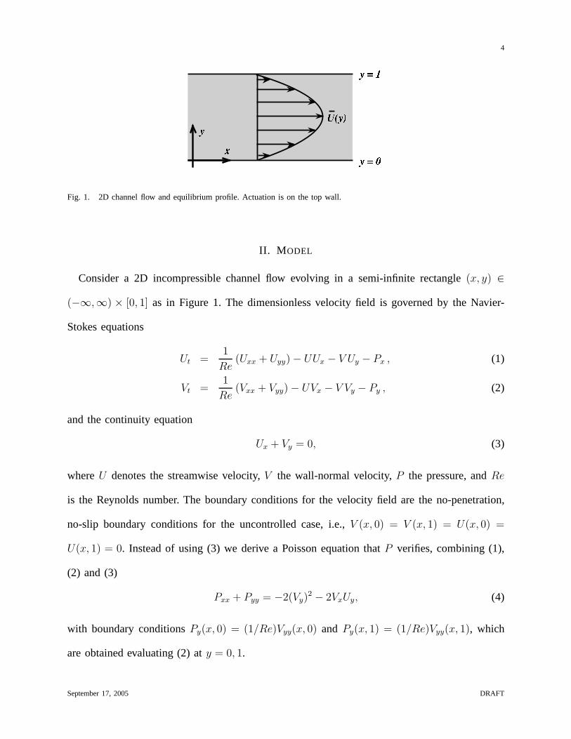
xy U ( y )Fig. 1. 2D channel flow and equilibrium profile. Actuation is on the top wall.
II. M ODEL
Consider a 2D incompressible channel flow evolving in a semi-infinite rectangle(x, y) ∈
(−∞,∞) × [0, 1] as in Figure 1. The dimensionless velocity field is governed by the Navier-
Stokes equations
Ut =1
Re(Uxx + Uyy) − UUx − V Uy − Px , (1)
Vt =1
Re(Vxx + Vyy) − UVx − V Vy − Py , (2)
and the continuity equation
Ux + Vy = 0, (3)
whereU denotes the streamwise velocity,V the wall-normal velocity,P the pressure, andRe
is the Reynolds number. The boundary conditions for the velocity field are the no-penetration,
no-slip boundary conditions for the uncontrolled case, i.e., V (x, 0) = V (x, 1) = U(x, 0) =
U(x, 1) = 0. Instead of using (3) we derive a Poisson equation thatP verifies, combining (1),
(2) and (3)
Pxx + Pyy = −2(Vy)2 − 2VxUy, (4)
with boundary conditionsPy(x, 0) = (1/Re)Vyy(x, 0) and Py(x, 1) = (1/Re)Vyy(x, 1), which
are obtained evaluating (2) aty = 0, 1.
September 17, 2005 DRAFT
Page 5
5
The equilibrium solution of (1)–(3) is the parabolic Poisseuille profile
Ue = 4y(1 − y), (5)
V e = 0, (6)
P e = P0 −8
Rex, (7)
shown in Figure 1. This equilibrium is unstable for high Reynolds numbers [19]. Defining the
fluctuation variablesu = U −Ue andp = P −P e, and linearizing around the equilibrium profile
(5)–(7), the plant equations become the Stokes equations
ut =1
Re(uxx + uyy) + 4y(y − 1)ux + 4(2y − 1)V − px, (8)
Vt =1
Re(Vxx + Vyy) + 4y(y − 1)Vx − py, (9)
pxx + pyy = 8(2y − 1)Vx, (10)
with boundary conditions
u(x, 0) = 0, (11)
u(x, 1) = Uc(x), (12)
V (x, 0) = 0, (13)
V (x, 1) = Vc(x), (14)
py(x, 0) =Vyy(x, 0)
Re, (15)
py(x, 1) =Vyy(x, 1) + (Vc)xx(x)
Re− (Vc)t(x). (16)
The continuity equation is still verified
ux + Vy = 0. (17)
We have added in (12) and (14) the actuation variablesUc(x) and Vc(x), respectively for
streamwise and normal velocity boundary control. The actuators are placed along the top wall,
September 17, 2005 DRAFT
Page 6
6
y = 1, and we assume they can be independently actuated for allx ∈ R. No actuation is done
inside the channel or at the bottom wall.
Taking Laplacian in equation (9) and using (10), we get an autonomous equation for the
normal velocity, the well-known Orr-Sommerfeld equation,
△Vt =1
Re△2V + 4y(y − 1)△Vx − 8Vx, (18)
with boundary conditions (13)–(14), as well asVy(x, 0) = 0, Vy(x, 1) = −(Uc)x, derived from
(11)–(12) and (17). This equation is numerically studied inhydrodynamic theory to determine
stability of the channel flow [17].
Defining Y = −Vy, it is possible to partially solve (18) and obtain an evolution equation for
Y ,
Yt =1
Re(Yxx + Yyy) + 4y(y − 1)Yx +
∫ y
0
∫ ∞
−∞
Y (ξ, η)
∫ ∞
−∞
16πke2πik(x−ξ)
× [πk(2y − 1) − 2 sinh (2πk(y − η)) 2πk(2η − 1) cosh (2πk(y − η))] dkdξdη
+
∫ 1
0
∫ ∞
−∞
Y (ξ, η)
∫ ∞
−∞
32πke2πik(x−ξ) cosh (2πky)
sinh (2πk)[cosh (2πk(1 − η))
+πk(2η − 1) sinh (2πk(1 − η))] dkdξdη
+
∫ ∞
−∞
∫ ∞
−∞
(
Yy(ξ, 1) − (Vc)xx(ξ)
Re+ (Vc)t(ξ)
)
2πke2πik(x−ξ) cosh (2πky)
sinh (2πk)dkdξ
−
∫ ∞
−∞
∫ ∞
−∞
Yy(ξ, 0)
Re2πke2πik(x−ξ) cosh (2πk(1 − y))
sinh (2πk)dkdξ, (19)
with boundary conditionsYy(x, 0) = 0 andY (x, 1) = (Uc)x. Equation (19) governs the channel
flow, since fromY and using (17), we recover both components of the velocity field:
V (x, y) = −
∫ y
0
Y (x, η)dη, (20)
u(x, y) =
∫ x
−∞
Y (ξ, y)dξ. (21)
Equation (19) displays the full complexity of the Navier-Stokes dynamics, which the PDE
system (8)–(10) conceals through the presence of the pressure equation (10), and the Orr-
September 17, 2005 DRAFT
Page 7
7
Sommerfeld equation (18) conceals through the use of fourthorder derivatives. Besides being
unstable (for high Reynolds numbers), theY system incorporates (on its right-hand side) the
components ofY (x, y) from everywhere in the domain. This is the main source of difficulty
for both controlling and solving the Navier-Stokes equations. A perturbation somewhere in the
flow is instantaneously felt everywhere—a consequence of the incompressible nature of the flow.
Our approach to overcoming this obstacle is to use one of the two control variables (normal
velocityVc(x), which is incorporated explicitly inside the equation) to prevent perturbations from
propagating in the direction from the controlled boundary towards the uncontrolled boundary.
This is a sort of “spatial causality” ony, which in the nonlinear control literature is referred to
as the ‘strict-feedback structure’ [14].
III. CONTROLLER
The explicit control law consists of two parts—the normal velocity controllerVc(x) and the
streamwise velocity controllerUc(x). Vc(x) makes the integral operator in the third to fifth lines of
(19) spatially causal iny,1 which is a necessary structure for the application of a “backstepping”
boundary controller for stabilization of spatially causalpartial integro-differential equations [20].
Uc(x) is a backstepping controller which stabilizes the spatially causal structure imposed by
Vc(x). The expressions for the control laws are
Uc(t, x) =
∫ 1
0
∫ ∞
−∞
Qu(x − ξ, η)u(t, ξ, η)dξdη, (22)
Vc(t, x) = h(t, x), (23)
whereh verifies the equation
ht = hxx + g(t, x), (24)
1The first, second and sixth lines are already spatially causal in y.
September 17, 2005 DRAFT
Page 8
8
where
g =
∫ 1
0
∫ ∞
−∞
QV (x − ξ, η)V (t, ξ, η)dξdη
+
∫ ∞
−∞
Q0(x − ξ) (uy(t, ξ, 0) − uy(t, ξ, 1))dξ, (25)
and the kernelsQu, QV andQ0 are defined as
Qu =
∫ ∞
−∞
χ(k)K(k, 1, η)e2πik(x−ξ)dk, (26)
QV =
∫ ∞
−∞
χ(k)16πki(2η − 1) cosh (2πk(1 − η)) e2πik(x−ξ)dk, (27)
Q0 =
∫ ∞
−∞
χ(k)2πki
Ree2πik(x−ξ)dk. (28)
In expressions (26)–(28),χ(k) is a truncating function in the wave number space whose
definition is
χ(k) =
1, m < |k| < M
0, otherwise(29)
wherem andM are respectively the low and high cut-off wave numbers, two design parameters
which can be conservatively chosen asm ≤ 132πRe
and M ≥ 1π
√
Re2
. The functionK(k, y, η)
appearing in (26) is a (complex valued) gain kernel defined as
K(k, y, η) = limn→∞
Kn(k, y, η), (30)
September 17, 2005 DRAFT
Page 9
9
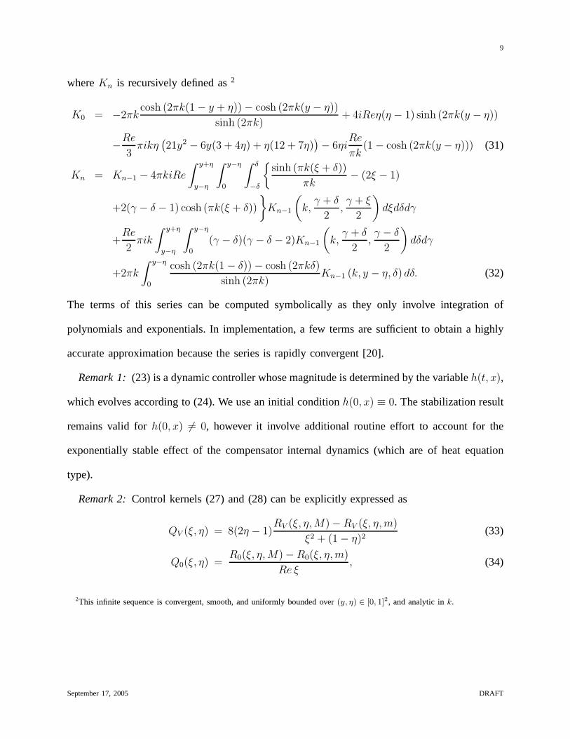
whereKn is recursively defined as2
K0 = −2πkcosh (2πk(1 − y + η)) − cosh (2πk(y − η))
sinh (2πk)+ 4iReη(η − 1) sinh (2πk(y − η))
−Re
3πikη
(
21y2 − 6y(3 + 4η) + η(12 + 7η))
− 6ηiRe
πk(1 − cosh (2πk(y − η))) (31)
Kn = Kn−1 − 4πkiRe
∫ y+η
y−η
∫ y−η
0
∫ δ
−δ
{
sinh (πk(ξ + δ))
πk− (2ξ − 1)
+2(γ − δ − 1) cosh (πk(ξ + δ))
}
Kn−1
(
k,γ + δ
2,γ + ξ
2
)
dξdδdγ
+Re
2πik
∫ y+η
y−η
∫ y−η
0
(γ − δ)(γ − δ − 2)Kn−1
(
k,γ + δ
2,γ − δ
2
)
dδdγ
+2πk
∫ y−η
0
cosh (2πk(1 − δ)) − cosh (2πkδ)
sinh (2πk)Kn−1 (k, y − η, δ) dδ. (32)
The terms of this series can be computed symbolically as theyonly involve integration of
polynomials and exponentials. In implementation, a few terms are sufficient to obtain a highly
accurate approximation because the series is rapidly convergent [20].
Remark 1: (23) is a dynamic controller whose magnitude is determined by the variableh(t, x),
which evolves according to (24). We use an initial conditionh(0, x) ≡ 0. The stabilization result
remains valid forh(0, x) 6= 0, however it involve additional routine effort to account for the
exponentially stable effect of the compensator internal dynamics (which are of heat equation
type).
Remark 2: Control kernels (27) and (28) can be explicitly expressed as
QV (ξ, η) = 8(2η − 1)RV (ξ, η, M) − RV (ξ, η, m)
ξ2 + (1 − η)2(33)
Q0(ξ, η) =R0(ξ, η, M) − R0(ξ, η, m)
Re ξ, (34)
2This infinite sequence is convergent, smooth, and uniformlybounded over(y, η) ∈ [0, 1]2, and analytic ink.
September 17, 2005 DRAFT
Page 10
10
whereRV (ξ, η, k) andR0(ξ, η, k) are defined
RV =((1 − η)2− ξ2)sin(2πkξ)cosh(2πk(1 − η))
2π(ξ2 + (1 − η)2)+ kξ cos (2πkξ) cosh (2πk(1 − η))
−ξ(1 − η) cos (2πkξ) sinh (2πk(1 − η))
π(ξ2 + (1 − η)2)− k(1 − η) sin(2πkξ) sinh(2πk(1 − η)) (35)
R0 = k cos (2πkξ) −sin (2πkξ)
2πξ. (36)
IV. M AIN RESULTS
Due to the explicit form of the controller, the solution of the closed loop system is also
obtained in the explicit form,
u(t, x, y) = u∗(t, x, y) + ǫu(t, x, y), (37)
V (t, x, y) = V ∗(t, x, y) + ǫV (t, x, y), (38)
where
u∗ = 2∞
∑
j=1
∫ ∞
−∞
∫ ∞
−∞
χ(k)e−t4k2π2
+π2j2
Re+2πik(x−ξ)
[
sin (πjy) +
∫ y
0
L(k, y, η) sin (πjη) dη
]
×
∫ 1
0
[
sin (πjη) −
∫ 1
η
K(k, σ, η) sin (πjσ) dσ
]
u(0, ξ, η)dηdξdk , (39)
V ∗ = −2∞
∑
j=1
∫ ∞
−∞
∫ ∞
−∞
χ(k)e−t4k2π2
+π2j2
Re+2πik(x−ξ)
[∫ y
0
(∫ y
η
L(k, σ, η)dσ
)
sin (πjη) dη
+1 − cos (πjy)
πj
]∫ 1
0
[
πj cos (πjη) + K(k, η, η) sin (πjη) −
∫ 1
η
Kη(k, σ, η)
× sin (πjσ) dσ
]
V (0, ξ, η)dηdξdk. (40)
The variablesǫu(t, x, y) and ǫV (t, x, y) represent the error of approximation of the velocity
field and are bounded in the following way
||ǫu(t)||2L2 + ||ǫV (t)||2L2 ≤ e−
Re4
t(
||ǫu(0)||2L2 + ||ǫV (0)||2L2
)
, (41)
September 17, 2005 DRAFT
Page 11
11
where bothǫu(0, x, y) and ǫV (0, x, y) can be written in terms of the initial conditions of the
velocity field as
ǫu(0, x, y) = u(0, x, y)−
∫ ∞
−∞
sin (2πMξ) − sin (2πmξ)
πξu(0, x− ξ, y)dξ, (42)
ǫV (0, x, y) = V (0, x, y) −
∫ ∞
−∞
sin (2πMξ) − sin (2πmξ)
πξV (0, x − ξ, y)dξ, (43)
The bound on the errors is proportional to the initial kinetic energy ofǫu and ǫV , which, as
made explicit in the expressions (42)–(43), is in turn proportional to the kinetic energy ofu and
V at very small and very large length scales (the integral thatwe are substacting from the initial
conditions represents the intermediate length scale content), and decays exponentially. Therefore,
this initial energy will typically be a very small fraction of the overall kinetic energy, making
the errorsǫu and ǫV very small in comparison withu∗ andV ∗ respectively.
The kernelL in (39) is defined as a convergent, smooth sequence of fuctions
L(k, y, η) = limn→∞
Ln(k, y, η), (44)
whose terms are recursively defined as
L0 = K0, (45)
Ln = Ln−1 + 4iRe
∫ y+η
y−η
∫ y−η
0
∫ δ
−δ
{2πk(γ + ξ − 1) × cosh (πk(ξ − δ)) + sinh (πk(ξ − δ))
−πk(2δ − 1)}Ln−1
(
k,γ + ξ
2,γ − δ
2
)
dξdδdγ
−Re
2πik
∫ y+η
y−η
∫ y−η
0
(γ + δ)(γ + δ − 2)Ln−1
(
k,γ + δ
2,γ − δ
2
)
dδdγ . (46)
Control laws (22)–(32) guarantee the following results.
Theorem 1: The equilibriumu(x, y) ≡ V (x, y) ≡ 0 of system (8)–(16), (22)–(32) is expo-
nentially stable in theL2, H1 andH2 sense. Moreover, the solutions foru(t, x, y) andV (t, x, y)
are given explicitly by (37)–(46).
September 17, 2005 DRAFT
Page 12
12
Theorem 2: Control lawsUc, Vc and kernelsQu, QV , Q0, as defined by (22)–(32), have the
following properties:
i) Uc andVc are spatially invariant inx.
ii)∫ ∞
−∞Vc(t, ξ)dξ = 0 (zero net flux).
iii) |Q| ≤ C/|x − ξ|, for Q = Qu, QV , Q0.
iv) Uc andVc are smooth functions ofx.
v) Qu, QV , Q0 are real valued.
vi) Qu, QV , Q0 are smooth in their arguments.
vii) Uc andVc areL2 functions ofx.
viii) All spatial derivatives ofUc andVc areL2 function of x.
Remark 3: Theorem 1, stated for the linearized equations (8)–(9), is valid for the nonlinear
equations (1)–(2) in alocal sense, i.e., provided that the initial data are sufficientlyclose (in the
appropiate norm) to the equilibrium (5)–(7).
Remark 4: By Sobolev’s Embedding Theorem [22],H2 stability suffices to establish conti-
nuity of the velocity field when the domain is bounded. The argument is not applicable to the
infinite channel, but it holds if the channel is periodic, a setting for which our results extend
trivially.
Remark 5: Theorem 2 ensures that the control laws are well behaved. Property i, spatial
invariance, means that the feedback operators commute withtranslations in thex direction [6],
which is crucial for implementation. Property ii ensures that we do not violate the physical
restriction of zero net flux, which is derived from mass conservation. Property iii allows to
truncate the integrals with respect toξ to the vicinity ofx, which allows sensing to be restricted
just to a neighborhood (in thex direction) of the actuator. Properties iv to vi ensure that the
control laws are well defined. Properties vii and viii prove finiteness of energy of the controllers
and their spatial derivatives.
September 17, 2005 DRAFT
Page 13
13
The next sections are devoted to proving these theorems.
V. L2 STABILITY AND EXPLICIT SOLUTIONS
As common for infinite channels, we use a Fourier transform inx. The transform pair (direct
and inverse transform) has the following definition:
f(k, y) =
∫ ∞
−∞
f(x, y)e−2πikxdx, (47)
f(x, y) =
∫ ∞
−∞
f(k, y)e2πikxdk. (48)
Note that we use the same symbolf for both the originalf(x, y) and the imagef(k, y). In
hydrodynamics,k is referred to as the “wave number.”
One property of the Fourier transform is that theL2 norm is the same in Fourier space as in
physical space, i.e.,
||f ||2L2=
∫ 1
0
∫ ∞
−∞
f 2(k, y)dkdy =
∫ 1
0
∫ ∞
−∞
f 2(x, y)dxdy, (49)
allowing us to deriveL2 exponential stability in physical space from the same property in Fourier
space. This result is called Parseval’s formula in the literature [8].
We also define theL2 norm of f(k, y) with respect toy:
||f(k)||2L2 =
∫ 1
0
|f(k, y)|2dy. (50)
The L2 norm as a function ofk is related to theL2 norm as
||f ||2L2 =
∫ ∞
−∞
||f(k)||2L2dk (51)
Equations (8)–(10) written in the Fourier domain are
ut =−4π2k2u + uyy
Re+ 8kπiy(y − 1)u + 4(2y − 1)V − 2πikp, (52)
Vt =−4π2k2V + Vyy
Re+ 8πkiy(y − 1)V − py, (53)
−4π2k2p + pyy = 16πki(2y − 1)V, (54)
September 17, 2005 DRAFT
Page 14
14
with boundary conditions
u(k, 0) = 0, (55)
u(k, 1) = Uc(k), (56)
V (k, 0) = 0, (57)
V (k, 1) = Vc(k), (58)
py(k, 0) =Vyy(k, 0)
Re, (59)
py(k, 1) =Vyy(k, 1) − 4π2k2Vc(k)
Re− (Vc)t(k), (60)
and the continuity equation (17) is now
2πkiu(k, y) + Vy(k, y) = 0. (61)
Thanks to linearity and spatial invariance, there is no coupling between different wave numbers.
This allows us to consider the equations for each wave numberindependently. Then, the main
idea behind the design of the controller is to consider two different cases depending on the wave
numberk. For wave numbersm < |k| < M , which we will refer to ascontrolled wave numbers,
we will design a backstepping controller that achieves stabilization, whereas for wave numbers
in the range|k| ≥ M or in the range|k| ≤ m, which we will call uncontrolled wave numbers,
the system is left without control but is exponentially stable. This is a well-known fact from
hydrodynamic stability theory [19].
Estimates ofm andM are found in the paper based on Lyapunov analysis and allow usto use
feedback for only the wave numbersm < |k| < M . This is crucial because feedback over the
entire infinite range ofk’s would not be convergent. The truncations atk = m, M are truncations
in Fourier space which do not result in a discontinuity inx.
We now analyze equations (52)–(54) in detail, for both controlled and uncontrolled wave
numbers.
September 17, 2005 DRAFT
Page 15
15
A. Controlled wave numbers
For m < |k| < M we first solve (54) in order to eliminate the pressure. The equation can be
easily solved since it is just an ODE iny, for eachk. Introducing its solution into (52), we are
left with
ut =1
Re
(
−4π2k2u + uyy
)
+ 8πkiy(y − 1)u + 4(2y − 1)V
+16πk
∫ y
0
V (k, η)(2η − 1) sinh (2πk(y − η)) dη + icosh (2πk(1 − y))
sinh (2πk)
Vyy(k, 0)
Re
−16πkcosh (2πky)
sinh (2πk)
∫ 1
0
V (k, η)(2η − 1) cosh (2πk(1 − η)) dη
−icosh (2πky)
sinh (2πk)
(
Vyy(k, 1) − 4π2k2Vc(k)
Re− (Vc)t(k)
)
. (62)
We don’t need to separately write and control theV equation because, by the continuity equation
(61) and using the fact thatV (k, 0) = 0, we can writeV in terms ofu
V (k, y) =
∫ y
0
Vy(k, η)dη = −2πki
∫ y
0
u(k, η)dη. (63)
Introducing (63) in (62), and simplifying the resulting double integral by changing the order of
integration, we reduce (62) to an autonomous equation that governs the whole velocity field.
This equation is
ut =1
Re
(
−4π2k2u + uyy
)
+ 8πkiy(y − 1)u +2πk cosh (2πk(1 − y))
sinh (2πk)
uy(k, 0)
Re
+8i
∫ y
0
{πk(2y − 1) − 2 sinh (2πk(y − η)) − 2πk(2η − 1) cosh (2πk(y − η))} u(k, η)dη
+16icosh (2πky)
sinh (2πk)
∫ 1
0
{cosh (2πk(1 − η))πk(2η − 1) sinh (2πk(1 − η))} u(k, η)dη
+icosh (2πky)
sinh (2πk)
(
2πkiuy(k, 1) + 4π2k2Vc(k)
Re+ (Vc)t(k)
)
, (64)
with boundary conditions
u(k, 0) = 0, (65)
u(k, 1) = Uc(k). (66)
September 17, 2005 DRAFT
Page 16
16
Note that the relation betweenY in (19) andu in (64) is thatY (k, y) = 2πkiu(k, y).
Now, we design the controller in two steps. First, we setVc so that (64) has a strict-feedback
form in the sense previously defined:
(Vc)t =2πki (uy(k, 0) − uy(k, 1)) − 4π2k2Vc
Re
−16πki
∫ 1
0
(2η − 1)V (k, η) cosh (2πk(1 − η)) dη. (67)
This can be integrated and explicitly stated as a dynamic controller in the Laplace domain:
Vc =2πki
s + 4π2k2
Re
[
uy(s, k, 0) − uy(s, k, 1)
Re
× −8
∫ 1
0
(2η − 1)V (s, k, η) cosh (2πk(1 − η)) dη
]
. (68)
Control law (67) can be expressed in the time domain and physical space as (23)–(25) and (27),
(28), by use of the convolution theorem of the Fourier transform.
IntroducingVc in (64) yields
ut =1
Re
(
−4π2k2u + uyy
)
+ 8πkiy(y − 1)u
+8i
∫ y
0
{πk(2y − 1) − 2 sinh (2πk(y − η)) − 2πk(2η − 1) cosh (2πk(y − η))} u(k, η)dη
−2πkcosh (2πky) − cosh (2πk(1 − y))
sinh (2πk)
uy(k, 0)
Re. (69)
Equation (69) can be stabilized using the backstepping technique for parabolic partial integro-
differential equations [20]. Using backstepping, we mapu, for each wave numberm < |k| < M ,
into the family of heat equations
αt =1
Re
(
−4π2k2α + αyy
)
, (70)
α(k, 0) = 0 , (71)
α(k, 1) = 0 , (72)
September 17, 2005 DRAFT
Page 17
17
where
α = u −
∫ y
0
K(k, y, η)u(t, k, η)dη , (73)
u = α +
∫ y
0
L(k, y, η)α(t, k, η)dη , (74)
are respectively the direct and inverse transformation. The kernel K is found to verify the
following equation
1
ReKyy =
1
ReKηη + 8πikη(η − 1)K − 8i {πk(2y − 1) − sinh (2πk(y − η))
−2πk(2η − 1) cosh (2πk(y − η))} + 8i
∫ y
η
{πk(2ξ − 1) − 2 sinh (2πk(ξ − η))
−2πk(2η − 1) cosh (2πk(ξ − η))}K(k, y, ξ)dξ, (75)
a hyperbolic partial integro-differential equation (PIDE) in the regionT = {(y, η) : 0 ≤ η ≤
y ≤ 1} with boundary conditions:
K(y, y) = −2Re
3πiky2(2y − 3) − 2πk
cosh (2πk) − 1
sinh (2πk), (76)
K(y, 0) =2πk
sinh (2πk)
{
cosh (2πky) − cosh (2πk(1 − y))
+
∫ y
0
K(k, y, ξ) [cosh (2πk(1 − ξ)) − cosh (2πkξ)] dξ
}
. (77)
The equation can be transformed into an integral equation for calculating the kernel symbolically.
To do this, we transform the PIDE into an integral equation and solve it explicitly via a successive
approximation series. The series definition ofK is (30)–(32). We skip the details, since we follow
[20] exactly, with the only difference that the kernel is complex valued, which does not change
the proof. In addition, using the estimates of the proof and the fact that the terms in the series
definition (31)–(32) ofK are analytic ink, it can be shown that the kernel itself is also analytic
as a complex function ofk, for any boundedk [18], so in particular, it will be analytic in the
annulusm < |k| < M .
September 17, 2005 DRAFT
Page 18
18
From the transformation (73) and the boundary condition (65) the control law is
Uc =
∫ 1
0
K(k, 1, η)u(t, k, η)dη. (78)
Using the convolution theorem of the Fourier transform we write the control law (78) back
in physical space. The resulting expressions is (22).
The equation for the inverse kernelL in (74) is similar to the one ofK and enjoys similar
properties
1
ReLyy =
1
ReLηη − 8πiky(y − 1)L − 8i {πk(2y − 1) − 2 sinh (2πk(y − η))
−2πk(2η − 1) cosh (2πk(y − η))} − 8i
∫ y
η
{πk(2y − 1) − sinh (2πk(y − ξ))
+2πk(2ξ − 1) cosh (2πk(y − ξ))}L(k, ξ, η)dξ, (79)
again a hyperbolic partial integro-differential equationin the regionT with boundary conditions
L(y, y) = −2Re
3πiky2(2y − 3) − 2πk
cosh (2πk) − 1
sinh (2πk), (80)
L(y, 0) =2πk
sinh (2πk)
{
cosh (2πky) − cosh (2πk(1 − y))
}
. (81)
The equation can be transformed into an integral equation and calculated via the successive
approximation series (45)–(46).
By using (63) and (73)–(74),V can also be expressed in terms ofα
α = iVy −
∫ y
0K(k, y, η)Vy(t, k, η)dη
2πk(82)
V = −2πki
∫ y
0
[
1 +
∫ y
η
L(k, η, σ)dσ
]
α(t, k, η)dη . (83)
Since we can solve the heat equation (70)–(72) explicitly, the inverse transformations (74) and
(83) yield the explicit solutionsu∗(t, k, y) andV ∗(t, k, y), respectively.
Moreover, since (73)–(74) map (69) into (70), stability properties of the velocity field follows
from those of theα system.
September 17, 2005 DRAFT
Page 19
19
Proposition 1: For anyk in the rangem < |k| < M , the equilibriumu(t, k, y) ≡ V (t, k, y) ≡
0 of the system (52)–(60) with feedback control laws (67), (78) is exponentially stable in the
L2 sense, i.e.,
||V (t, k)||2L2 + ||u(t, k)||2
L2 ≤ D0e−1
2Ret(
||V (0, k)||2L2 + ||u(0, k)||2
L2
)
, (84)
whereD0 is defined as:
D0 = (1 + 4π2M2) maxm<|k|<M
{(1 + ||L||∞)2(1 + ||K||∞)2}. (85)
Proof: First, from theα equation (70) it is possible to get anL2 estimate
||α(t, k)||2L2 ≤ e−
1
2Ret||α(0, k)||2
L2, (86)
then employing the direct and inverse transformations (73)–(74) and (83) we get (84)–(85).
Now, if we apply the feedback laws (67), (78) forall wave numbersm < |k| < M , then the
control laws in physical space are given by expressions (22)–(28), where the inverse transform
integrals are truncated atk = m, M in (26)–(28). If we define
V ∗(t, x, y) =
∫ ∞
−∞
χ(k)V (t, k, y)e2πikxdk, (87)
u∗(t, x, y) =
∫ ∞
−∞
χ(k)u(t, k, y)e2πikxdk, (88)
which are variables that contain all velocity field information for wave numbersm < |k| < M ,
the following result holds.
Proposition 2: Consider equations (8)–(16) with control laws (22)–(23). Then the variables
u∗(t, x, y) andV ∗(t, x, y) defined in (87)–(88) decay exponentially:
||V ∗(t)||2L2 + ||u∗(t)||2L2 ≤ D0e−1
2Ret(
||V ∗(0)||2L2 + ||u∗(0)||2L2
)
. (89)
Proof: The Fourier transform of the star variables is, by definition, the same as the Fourier
transform of the original variables form < |k| < M , and zero otherwise. Therefore, applying
September 17, 2005 DRAFT
Page 20
20
Parseval’s formula and Proposition 1,
||V ∗(t)||2L2 + ||u∗(t)||2L2 =
∫ ∞
−∞
(
||V ∗(t, k)||2L2 + ||u∗(t, k)||2
L2
)
dk
=
∫ ∞
−∞
χ(k)(
||V (t, k)||2L2 + ||u(t, k)||2
L2
)
dk
≤ D0e−1
2Ret
∫ ∞
−∞
χ(k)(
||V (0, k)||2L2 + ||u(0, k)||2
L2
)
dk
= D0e− 1
2Ret(
||V ∗(0)||2L2 + ||u∗(0)||2L2
)
, (90)
proving (89).
B. Uncontrolled wave number analysis
For the uncontrolled system (52)–(53), we define, for eachk, the Lyapunov functional
Λ(k, t) =1
2
(
||V (t, k)||2L2 + ||u(t, k)||2
L2
)
(91)
The time derivative ofΛ is
Λ = −8π2k2
ReΛ −
1
Re
(
||uy(k)||2L2 + ||Vy(k)||2
L2
)
+ 4
∫ 1
0
(2y − 1)uV + uV
2dy, (92)
where the bar denotes the complex conjugate, and the pressure term has disappeared using
integration by parts and the continuity equation (61). The second term in the first line of (92)
can also be bounded using the Poincare inequality, thanks tothe Dirichlet boundary condition
at y = 0:
−||uy(k)||2L2 − ||Vy(k)||2
L2 ≤ −Λ
2. (93)
Consider now separately the two cases|k| ≤ m and |k| ≥ M . In the first case, we can bound
the second line of (92) as
Λ ≤ −8π2k2
ReΛ −
1
2ReΛ + 4Λ, (94)
so, if |k| ≥ 1π
√
Re2
, then
Λ ≤ −1
2ReΛ. (95)
September 17, 2005 DRAFT
Page 21
21
Now, consider the case of small wave numbers. We bound the second line of (92) using the
continuity equation (61)
Λ ≤ −8π2k2
ReΛ −
1
2ReΛ + 8π|k|Λ, (96)
so, if |k| ≤ 132πRe
, then
Λ ≤ −1
4ReΛ. (97)
We have just proved the following result:
Proposition 3: If m = 132πRe
and M = 1π
√
Re2
, then for both|k| ≤ m and |k| ≥ M the
equilibrium u(t, k, y) ≡ V (t, k, y) ≡ 0 of the uncontrolled system (52)–(60) is exponentially
stable in theL2 sense:
||V (t, k)||2L2 + ||u(t, k)||2
L2 ≤ e−1
4Ret(
||V (0, k)||2L2 + ||u(0, k)||2
L2
)
. (98)
Since the decay rate in (98) is independent ofk, that allows us to claim the following result
for all uncontrolled wave numbers.
Proposition 4: The variablesǫu(t, x, y) and ǫV (t, x, y) defined as
ǫu(t, x, y) =
∫ ∞
−∞
(1 − χ(k)) u(t, k, y)e2πikxdk, (99)
ǫV (t, x, y) =
∫ ∞
−∞
(1 − χ(k)) V (t, k, y)e2πikxdk, (100)
decay exponentially as
||ǫV (t)||2L2 + ||ǫu(t)||2L2 ≤ e
−1
4Ret(
||ǫV (0)||2L2 + ||ǫu(0)||2L2
)
. (101)
Proof: As in Proposition 2.
September 17, 2005 DRAFT
Page 22
22
C. Analysis for the entire wave number range
Using (37)–(38),
||V (t)||2L2 =
∫ ∞
−∞
||V (t, k)||2L2dk
=
∫ 1
0
∫ ∞
−∞
(V ∗(t, k, y) + ǫV (t, k, y))2 dkdy
=
∫ 1
0
∫ ∞
−∞
(
(V ∗)2 + ǫ2V + 2V ∗ǫV
)
dkdy
= ||V ∗(t)||2L2 + ||ǫV (t)||2L2, (102)
where we have used the fact thatV ∗(t, k, y)ǫV (t, k, y) = χ(k)(1−χ(k))V (t, k, y) andχ(k)(1−
χ(k)) is zero for allk by its definition (29).
This shows that theL2 norm of V is the sum of theL2 norms ofV ∗(t, k, y) and ǫV (t, k, y).
The same holds foru. Therefore, Theorem 1 follows from Propositions 2 and 4. Noting thatD0
as defined in (85) is greater than unity, we obtain the following estimate of the decay:
||V (t)||2L2 + ||u(t)||2L2 ≤ D0e−1
4Ret(
||V (0)||2L2 + ||u(0)||2L2
)
. (103)
The explicit solutions are (37)–(38), obtained by solving explicitly (70), using (74) and
(83), and applying the inverse Fourier transform, whereas the error bounds are obtained from
Proposition 4.
VI. H1 STABILITY
We define theH1 norm of f(x, y) as
||f ||2H1 = ||f ||2L2 + ||fx||2L2 + ||fy||
2L2. (104)
We also define theH1 norm of f(k, y) with respect to y as
||f(k)||2H1 = (1 + 4π2k2)||f(k)||2
L2 + ||fy(k)||2L2. (105)
September 17, 2005 DRAFT
Page 23
23
The H1 norm as a function ofk is related to theH1 norm as
||f ||2H1 =
∫ ∞
−∞
||f(k)||2H1dk. (106)
A. H1 stability for controlled wave numbers
For eachk, one has that
||f(k)||2H1 ≤ (5 + 16π2M2)||fy(k)||2
H1, (107)
where we have used (105) and Poincare’s inequality. This proves the equivalence, for anyk,
of the H1 norm of f(k, y) and theL2 norm of justfy(k, y). Therefore, we only have to show
exponential decay foruy andVy.
Due to the backstepping transformations (73), (74) and (82)(83),
αy = uy − K(k, y, y)u−
∫ y
0
Ky(k, y, η)u(t, k, η)dη , (108)
uy = αy + L(k, y, y)α +
∫ y
0
Ly(k, y, η)α(t, k, η)dη , (109)
α =−1
2πki
(
Vy −
∫ y
0
K(k, y, η)Vy(t, k, η)dη
)
, (110)
Vy = −2πki
(
α +
∫ y
0
L(k, y, η)α(t, k, η)dη
)
, (111)
and then it is possible to write the following estimates, which are derived from simple estimates
on α andαy from (70)
||uy(t, k)||2L2 ≤ D1e
− 2
5Ret||uy(0, k)||2
L2, (112)
||Vy(t, k)||2L2 ≤ D0e
− 1
2Ret||Vy(0, k)||2
L2, (113)
where
D1 = 5 maxm<|k|<M
{
(1 + 4||L||∞ + 4||Ly||∞)2(1 + 4||K||∞ + 4||Ky||∞)2
}
. (114)
Using these estimates the following proposition can be stated regarding the velocity field at each
k in the controlled range.
September 17, 2005 DRAFT
Page 24
24
Proposition 5: For anyk in the rangem < |k| < M , the equilibriumu(t, k, y) ≡ V (t, k, y) ≡
0 of the system (52)–(60) with feedback control laws (67), (78) is exponentially stable in the
H1 sense
||V (t, k)||2H1 + ||u(t, k)||2
H1 ≤ D2e−2
5Ret(
||V (0, k)||2H1 + ||u(0, k)||2
H1
)
, (115)
whereD2 is defined as:
D2 = (5 + 16π2M2) max{D0, D1}. (116)
Thanks to the same argument as in Proposition 2, forall wave numbersm < |k| < M , the
following result holds.
Proposition 6: Consider equations (8)–(16) with control laws (22)–(23). Then the variables
u∗(t, x, y) andV ∗(t, x, y) defined in (87)–(88) decay exponentially in theH1 norm:
||u∗(t)||2H1 + ||V ∗(t)||2H1 ≤ D2e−2
5Ret(
||u∗(0)||2H1 + ||V ∗(0)||2H1
)
. (117)
B. H1 stability for uncontrolled wave numbers
Following the same argument as in (91)–(97), a slightly different bound can be derived that
keeps some of theH1 norm in (96)
Λ ≤ −Λ
8Re−
ΛH
2Re, (118)
where
ΛH(k, t) =1
2
(
||uy(t, k)||2L2 + ||Vy(t, k)||2
L2
)
. (119)
September 17, 2005 DRAFT
Page 25
25
The time derivative ofΛH can be bounded as
dΛH
dt=
∫ 1
0
uyuyt + uyuyt + VyVyt + VyVyt
2dy
= −
∫ 1
0
uyyut + uyyut + VyyVt + VyyVt
2dy
= −1
Re
(
||uyy||2L2 + ||Vyy||
2L2
)
+ 4k2π2
∫ 1
0
uyyu + uyyu + VyyV + VyyV
2Redy
+2πki
∫ 1
0
uyyp − uyyp
2dy −
∫ 1
0
Vyypy + Vyypy
2dy − 4
∫ 1
0
(2y − 1)uyyV + uyyV
2dy
+8πki
∫ 1
0
y(y − 1)uyyu − uyyu − VyyV + VyyV
2dy, (120)
where we have used integration by parts and the Dirichlet boundary conditions of the uncontrolled
wave number range. Doing further integration by parts and using the divergence free condition,
we can simplify a little the previous expression:
dΛH
dt= −
1
Re
(
||uyy||2L2 + ||Vyy||
2L2
)
−8k2π2
ReΛh − 16π2k2
∫ 1
0
(2y − 1)uV − uV
2dy
−Vyyp + Vyyp
2
∣
∣
∣
∣
1
0
. (121)
Only the last term remains to be estimated. Using (59)–(60) with Vc being zero for uncontrolled
wave number, the last term in (121) can be expresssed as
Vyyp + Vyyp
2
∣
∣
∣
∣
1
0
= Repyp + pyp
2
∣
∣
∣
∣
1
0
. (122)
This quantity can be estimated using the following lemma.
Lemma 1: If the pressurep verifies the Poisson equation (54) with boundary conditions(59)–
(60), then
−pyp + pyp
2
∣
∣
∣
∣
1
0
≤ 16||V (t, k)||2L2. (123)
Proof: Multiplying equation (54) byp and integrating from zero to one, one gets:
−4π2k2||p(t, k)||2L2 +
∫ 1
0
ppyydy =
∫ 1
0
16πki(2y − 1)pV dy, (124)
September 17, 2005 DRAFT
Page 26
26
which integrated by parts, becomes
−ppy
∣
∣
∣
∣
1
0
= −4π2k2||p(t, k)||2L2 − ||py(t, k)||2
L2 −
∫ 1
0
16πki(2y − 1)pV dy. (125)
Now using Young’s inequality one finally arrives at
−ppy
∣
∣
∣
∣
1
0
≤ 16||V (t, k)||2L2. (126)
For the other conjugate pair one proceeds analogously, thuscompleting the proof.
Using the lemma, the time derivative ofΛH can be estimated as follows:
dΛH
dt≤ −
8k2π2
ReΛH + 16π2k2Λ + 16ReΛ. (127)
We take the following Lyapunov functional
ΛT = ΛH + (1 + 64Re2 + 4π2k2 + 64Reπ2k2)Λ, (128)
which is equivalent to theH1 norm, whose definition in terms ofΛ andΛH is
||u(t, k)||2H1 + ||V (t, k)||2
H1 = 2(1 + 4π2k2)Λ + 2ΛH . (129)
Computing the derivative of (128)
dΛT
dt≤ −
ΛH
2Re−
1 + 4π2k2
8ReΛ ≤ −d1ΛT , (130)
whered1 is a (possible very conservative) positive constant, whichdepends on the Reynolds
number (butnot on k)
d1 =1
8D3Re, (131)
and where
D3 = max{1 + 64Re2, 1 + 16Re}. (132)
Deriving an estimate of theH1 norm from this estimate forΛT , one reaches the following result.
September 17, 2005 DRAFT
Page 27
27
Proposition 7: If m = 132πRe
and M = 1π
√
Re2
, then for both|k| ≤ m and |k| ≥ M the
equilibrium u(t, k, y) ≡ V (t, k, y) ≡ 0 of the uncontrolled system (52)–(60) is exponentially
stable in theH1 sense:
||V (t, k)||2H1 + ||u(t, k)||2
H1 ≤ D3e−d1t
(
||V (0, k)||2H1 + ||u(0, k)||2
H1
)
. (133)
Since the decay rate in (133) is independent ofk, that allows us to claim the following result
for all uncontrolled wave numbers.
Proposition 8: The variablesǫu(t, x, y) and ǫV (t, x, y) defined as in (99)–(100) decay expo-
nentially in theH1 norm as
||ǫu(t)||2H1 + ||ǫV (t)||2H1 ≤ D3e
−d1t(
||ǫu(0)||2H1 + ||ǫV (0)||2H1
)
. (134)
C. Analysis for all wave numbers
From Propositions 6 and 8, and using the same argument as in Section V-C, theH1 stability
part of Theorem 1 is proved. One gets that
||u(t)||2H1 + ||V (t)||2H1 ≤ D4e−d1t
(
||u(0)||2H1 + ||V (0)||2H1
)
, (135)
whereD4 = max{D2, D3}.
VII. H2 STABILITY
The H2 norm of f(x, y) is defined as
||f ||2H2 = ||f ||2H1 + ||fxx||2L2 + ||fxy||
2L2 + ||fyy||
2L2 . (136)
We also define theH2 norm of f(k, y) with respect to y as
||f(k)||2H2 = ||f(k)||2
H1 + 16π4k4||f(k)||2L2 + 4π2k2||fy(k)||2
L2 + ||fyy(k)||2L2. (137)
The H2 norm as a function ofk is related to theH2 norm as
||f ||2H2 =
∫ ∞
−∞
||f(k)||2H2dk. (138)
September 17, 2005 DRAFT
Page 28
28
A. H2 stability for controlled wave numbers
Thanks to the backstepping transformations (73), (74) and (82), (83), one calculates the second
order derivative of bothu andV from α and its derivatives,
αyy = uyy − K(k, y, y)uy − (2Ky(k, y, y) + Kη(k, y, y))u
−
∫ y
0
Kyy(k, y, η)u(t, k, η)dη , (139)
uyy = αyy + L(k, y, y)αy + (2Ly(k, y, y) + Lη(k, y, y))α
+
∫ y
0
Lyy(k, y, η)α(t, k, η)dη , (140)
αy =−1
2πki
(
Vyy − K(k, y, y)Vy −
∫ y
0
Ky(k, y, η)Vy(t, k, η)dη
)
, (141)
Vyy = −2πki
(
αy + L(k, y, y)α +
∫ y
0
Ly(k, y, η)α(t, k, η)dη
)
. (142)
It is possible then to write the following estimates, which are derived from simple estimates on
α, αy andαyy from (70):
||u(t, k)||2H2 ≤ D5e
− 2
5Ret||u(0, k)||2
H2, (143)
||V (t, k)||2H2 ≤ D6e
− 2
5Ret||V (0, k)||2
H2. (144)
The positive constantsD5 andD6 are similarly defined to (114), only depending on the direct
and inverse kernels.
Using these estimates the following proposition can be stated regarding the velocity field at
eachk in the controlled range.
Proposition 9: For anyk in the rangem < |k| < M , the equilibriumu(t, k, y) ≡ V (t, k, y) ≡
0 of the system (52)–(60) with feedback control laws (67), (78) is exponentially stable in the
H2 sense
||V (t, k)||2H2 + ||u(t, k)||2
H2 ≤ D7e−2
5Ret(
||V (0, k)||2H2 + ||u(0, k)||2
H2
)
, (145)
September 17, 2005 DRAFT
Page 29
29
whereD7 is defined as:
D7 = max{D5, D6}. (146)
Thanks to the same argument as in Proposition 2, the following result holds forall wave
numbersm < |k| < M .
Proposition 10: Consider equations (8)–(16) with control laws (23)–(22). Then the variables
u∗(t, x, y) andV ∗(t, x, y) defined in (87)–(88) decay exponentially in theH2 norm:
||u∗(t)||2H2 + ||V ∗(t)||2H2 ≤ D8e−2
5Ret(
||u∗(0)||2H2 + ||V ∗(0)||2H2
)
. (147)
B. H2 stability for uncontrolled wave numbers
For the uncontrolled wave number range, thanks to the Dirichlet boundary conditions, theH2
norm ||u(t, k)||H2 is equivalent to the norm
||u(t, k)||2H1 +
∫ 1
0
∣
∣uyy(t, k, y) − 4π2k2u(t, k, y)∣
∣
2dy, (148)
i.e., to theH1 norm plus theL2 norm of the Laplacian, which we denote for short||△ku(k)||2L2
.
The proof of the norm equivalence is obtained integrating byparts,
||△ku(k)||2L2 =
∫ 1
0
∣
∣−4π2k2u(y, k) + uyy(y, k)∣
∣
2dy
=
∫ 1
0
[
16π4k4|u|2(y, k) + |uyy|2(y, k) − 4π2k2 (uuyy + uuyy)
]
dy
= 16π4k4||u(k)||2L2 + ||uyy(k)||2
L2 + 8π2k2||uy(k)||2L2. (149)
The next norm equivalence property is less obvious and we state it in the following lemma:
Lemma 2: Consideru andV verifying equations (52)–(53). Then, for the uncontrolledwave
number range, the norm||u||2H2
+ ||V ||2H2
is equivalent to the norm
||u||2H1 + ||V ||2
H1 + ||ut||2L2 + ||Vt||
2L2. (150)
This means the Laplacian operator in norm (148) can be replaced by a time derivative, when
considering theH2 norm of u andV together.
September 17, 2005 DRAFT
Page 30
30
Proof: Let us call
Λ1 = ||ut(t, k)||2L2 + ||Vt(t, k)||2
L2, (151)
Λ2 =||△ku(t, k)||2
L2+ ||△kV (t, k)||2
L2
Re2. (152)
Substituting in (151) equations (52)–(53),
Λ1 = Λ2 + Λ3, (153)
whereΛ3 contains the following terms
Λ3 = −
∫ 1
0
−2πki△kup + △kV py
Redy − 2πki
∫ 1
0
4y(1 − y)△kuu + △kV V
Redy
+
∫ 1
0
4(1 − 2y)△kuV
Redy −
∫ 1
0
(
2πkiput + pyVt
)
dy
+2πki
∫ 1
0
4y(1 − y)(
uut + vVt
)
dy +
∫ 1
0
4(1 − 2y) (V ut) dy. (154)
Now one can estimate this quantity:
|Λ3| ≤ 48(||u(k)||2H1 + ||V (k)||2
H1) +1
2(Λ1 + Λ2) , (155)
in which we have used integration by parts, Young’s inequality, and Lemma 1. Therefore:
||u||2H2 + ||V ||2
H2 ≤ D8
(
||u||2H1 + ||V ||2
H1 + Λ1
)
, (156)
and
||u||2H1 + ||V ||2
H1 + Λ1 ≤ D8
(
||u||2H2 + ||V ||2
H2
)
, (157)
whereD8 = 97 max{Re2, 1/Re2}.
From Lemma 2 one getsH2 stability for the uncontrolled wave numbers. This is obtained
by considering the norm||ut||2L2
+ ||Vt||2L2
as a Lyapunov functional whose derivative can be
bounded as
d
dt
||ut||2L2
+ ||Vt||2L2
2≤ −
1
4Re
(
||ut||2L2 + ||Vt||
2L2
)
, (158)
September 17, 2005 DRAFT
Page 31
31
which follows by taking the time derivative of (52)–(53) andapplying the same argument as for
L2 stability. Thus,
||ut(t, k)||2L2 + ||Vt(t, k)||2
L2 ≤ e−1
2Ret(
||ut(0, k)||2L2 + ||Vt(0, k)||2
L2
)
. (159)
Noting thatd1 ≤ 1/2Re and D3 ≥ 1, adding (159) to (133) and employing (156), (156) we
obtain the following result.
Proposition 11: If m = 132πRe
and M = 1π
√
Re2
, then for both|k| ≤ m and |k| ≥ M the
equilibrium u(t, k, y) ≡ V (t, k, y) ≡ 0 of the uncontrolled system (52)–(60) is exponentially
stable in theH2 sense:
||V (t, k)||2H2 + ||u(t, k)||2
H2 ≤ D28D3e
−d1t(
||V (0, k)||2H2 + ||u(0, k)||2
H2
)
. (160)
Since the decay rate in (160) is independent ofk, that allows us to claim the following result
for all uncontrolled wave numbers.
Proposition 12: The variablesǫu(t, x, y) andǫV (t, x, y) defined as in (99)–(100) decay expo-
nentially in theH2 norm as
||ǫu(t)||2H2 + ||ǫV (t)||2H2 ≤ D2
8D3e−d1t
(
||ǫu(0)||2H2 + ||ǫV (0)||2H2
)
. (161)
C. Analysis for all wave numbers
From Propositions 10 and 12, and again by the same argument asin Section V-C, theH2
stability part of Theorem 1 is proved. One gets that
||u(t)||2H2 + ||V (t)||2H2 ≤ D9e−d1t
(
||u(0)||2H2 + ||V (0)||2H2
)
, (162)
whereD9 = max{D7, D28D3}.
VIII. PROOF OFTHEOREM 2
Consider expressions (22)–(32).
September 17, 2005 DRAFT
Page 32
32
Points i and iv are deduced trivially from the fact that (22) and (25) are defined as convolutions,
and properties of the heat equation (24).
Point ii is verified if∫ ∞
−∞
Vc(t, x)dx = 0. (163)
From the definition of the Fourier transform ofVc,
Vc(t, k = 0) =
∫ ∞
−∞
Vc(t, x)dx. (164)
Therefore, ask = 0 lies on the uncontrolled wave number range−m < k < m, thenVc(t, k =
0) = 0 and the property is verified.
Point iii gives bounds on the decay rate of the kernels (26)–(28). All the kernel definitions
are of the form
Q(x − ξ, y) =
∫ ∞
−∞
χ(k)f(k, y)e2πik(x−ξ)dk, (165)
for somef analytic ink and smooth iny. Then, integrating by parts, we find that
|Q(x − ξ, y)| ≤(M − m)
π|x − ξ|max
m<|k|<M
∣
∣
∣
∣
df
dk(k, y)
∣
∣
∣
∣
+2
π|x − ξ|max
m<|k|<M|f(k, y)|
=C
|x − ξ|, (166)
showing that the kernels decay at least like1/|x− ξ|. This bound is made explicit in Remark 2
for QV andQ0.
From the definition of the inverse Fourier transform (48), itis straightforward to show that if
the real part off(k, y) is even and the imaginary part off(k, y) is odd, then the resultingf(x, y)
will always be real. Then, Point v can be proved showing that the functions under the integrals
in (26)–(28), which are inverse Fourier transforms, have this property. This is immediate for
(27) and (28). For (26), the property must be shown for the kernel K, defined by the sequence
(31)–(32). SinceK is the limit of the sequence, it will have the property if allKn share the
property. This can be proved by induction. ForK0, the property is evident from its definition
September 17, 2005 DRAFT
Page 33
33
(31) and can be immediately verified. ForKn, if the property is assumed forKn−1, then from
expression (32) and taking into account that the product of even functions is again even, the
product of odd functions is also even, and the product of an even function times an odd function
is odd, then it can be seen thatKn also shares the property. Therefore, the limitK will have a
real inverse transform, and kernelQu will be real.
Point vi is deduced from the definition of the kernels (26)–(28) as truncated Fourier inverse
integrals, which makes the kernels smooth inx−ξ. Smoothness inη is deduced from smoothness
of the functions under the integrals.
For Point vii, consider expression (22) and (26). Then,
||Uc||2L2 =
∫ ∞
−∞
Uc(t, x)2dx
=
∫ ∞
−∞
|Uc|(t, k)2dk
=
∫ ∞
−∞
χ(k)
∣
∣
∣
∣
∫ 1
0
K(k, 1, η)u(t, y, k)dη
∣
∣
∣
∣
2
dk
≤ 2(M − m) maxm≤|k|≤M
{||K||∞}||u(t)||2L2, (167)
and the result follows from Theorem 1.
On the other hand, forVc one has to use its dynamic equation (24)–(25), and a Lyapunov
functional consisting in half itsL2 norm. One then has, using Young’s inequality
d
dt
|Vc(k)|2
2≤
−π2k2
Re|Vc(k)|2 +
|uy|2(t, k, 0) + |uy|
2(t, k, 1)
Re
+64 cosh (2πM) ||V (t, k)||2L2, (168)
and supposing the control law is initialized at zero (see Remark 1), and using theH2 norm to
bound the second line of (168) one gets
|Vc(t, k)|2 ≤
∫ t
0
e−π2m2
Re(t−τ)
[
10||u(τ, k)||2
H2
Re+ 64 cosh (2πM) ||V (τ, k)||2
L2
]
dτ. (169)
September 17, 2005 DRAFT
Page 34
34
Integrating ink
||Vc(t)||2L2 ≤
∫ t
0
e−π2m2
Re(t−τ)
[
10||u(τ)||2H2
Re+ 64 cosh (2πM) ||V (τ)||2L2
]
dτ, (170)
and then the result follows from Theorem 1.
For Point viii, consider thejth spatial derivative ofUc and calculate itsL2 spatial norm
∣
∣
∣
∣
∣
∣
∣
∣
dj
dxjUc
∣
∣
∣
∣
∣
∣
∣
∣
2
L2
=
∫ ∞
−∞
(
dj
dxjUc(t, x)
)2
dx
=
∫ ∞
−∞
|2πk|2j|Uc|(t, k)2dk
≤ (2πM)2j ||Uc||2L2, (171)
so the result forUc follows from Point vii. We proceed similarly forVc, thus proving Point viii.
IX. D ISCUSSION
The result was presented in 2D for ease of notation. Since 3D channels are spatially invariant
in both streamwise and spanwise direction, it is possible toextend the design to 3D, by applying
the Fourier transform in both invariant directions and following the same steps, with some
refinements which include actuation of the spanwise velocity at the wall. The result also trivially
extends to periodic channel flow of arbitrary periodic box size, 2D or 3D; it only requires
substitution of the Fourier transform by Fourier series, with all other expressions still holding.
Our control laws are presented with full state feedback. However, for parabolic PDEs, in [21]
we developed an observer design methodology, which is dual to the backstepping control method-
ology in [20], which we extended to Navier-Stokes equationshere to solve the state feedback
stabilization problem for the channel flow. Extending the observer concepts in [21] to the Navier-
Stokes PDEs has allowed us to also develop an observer for thechannel flow, which is presented
in the conference paper [23]. While the observer is of interest in its own right (one can use it to
estimate turbulent flows without controlling/relaminarizing them), the state feedback controller in
September 17, 2005 DRAFT
Page 35
35
the present paper and the observer in [23] can be combined into an output feedback compensator,
which uses measurements ofP (x, 0) anduy(x, 0) only, and the actuation ofV (x, 1), u(x, 1).
Our controller requires actuation of both velocity components at the wall. An assumption
made throughout the flow control literature is that the boundary values of velocity are actuated
through micro-jet actuators that perform “zero-mean” blowing and suction. Effective actuation
of wall velocity at angles as low as5◦ relative to the wall has been demonstrated experimentally
using differentially actuated pairs of jets.
Unlike in our earlier publications [1], [5] where we included DNS simulation results that
demonstrated relaminarization with our controllers, we donot present simulation results in this
paper. In another publication, to be submitted to a fluid mechanics journal, we will present
an extension to 3D, without theH1, H2 stability estimates and without the explicit closed-loop
Navier-Stokes solutions (these two issues extend in a rather straightforward manner to 3D because
we deal with linearized Navier-Stokes equations), but withsimulations results included. The 3D
controller will include actuation in the spanwise direction. The numerical tests will focus on
turbulence-critical issues like the behavior of the controller at kx = 0 for moderate-to-largekz
and other issues which come up only in 3D.
ACKNOWLEDGEMENT
We thank Tom Bewley for numerous helpful discussions and expert advice, and Jennie Cochran
for reviewing the paper and correcting some analytical expressions.
REFERENCES
[1] O. M. Aamo and M. Krstic,Flow Control by Feedback: Stabilization and Mixing, Springer, 2002.
[2] O. M. Aamo, A. Smyshlyaev and M. Krstic, “Boundary control of the linearized Ginzburg-Landau model of vortex
shedding,”SIAM Journal of Control and Optimization, vol. 43, pp. 1953–1971, 2005.
[3] M.-R. Alam, W.-J. Liu and G. Haller, “Closed-loop separation control: an analytic approach,” submitted toPhys. Fluids,
2005.
September 17, 2005 DRAFT
Page 36
36
[4] J. Baker, A. Armaou and P.D. Christofides, “Nonlinear control of incompressible fluid flow: application to Burgers’ equation
and 2D channel flow,”Journal of Mathematical Analysis and Applications, vol. 252, pp. 230–255, 2000.
[5] A. Balogh, W.-J. Liu, and M. Krstic, “Stability enhancement by boundary control in 2D channel flow,”IEEE Transactions
on Automatic Control, vol. 46, pp. 1696–1711, 2001.
[6] B. Bamieh, F. Paganini and M.A. Dahleh, “Distributed control of spatially-invariant systems,”IEEE Trans. Automatic
Control, vol. 45, pp. 1091–1107, 2000.
[7] V. Barbu, “Feedback stabilization of Navier-Stokes equations,” ESAIM: Control, Optim. Cal. Var., vol. 9, pp. 197–205,
2003.
[8] R. Bracewell,The Fourier Transform and its Aplications, 3rd. ed., McGraw-Hill, 1999.
[9] J.-M. Coron, “On the controllability of the 2D incompressible Navier-Stokes equations with the Navier slip boundary
conditions,”ESAIM: Control, Optim. Cal. Var., vol. 1, pp. 35–75, 1996.
[10] C. Fabre, “Uniqueness results for Stokes equations andtheir consequences in linear and nonlinear control problems,”
ESAIM: Control, Optim. Cal. Var., vol. 1, pp. 267–302, 1996.
[11] M. Hogberg, T.R. Bewley and D.S. Henningson, “Linear feedback control and estimation of transition in plane channel
flow,” Journal of Fluid Mechanics, vol. 481, pp. 149-175, 2003.
[12] O.Y. Imanuvilov, “On exact controllability for the Navier-Stokes equations,”ESAIM: Control, Optim. Cal. Var., vol. 3, pp.
97–131, 1998.
[13] M. R. Jovanovic and B. Bamieh, “Componentwise energy amplification in channel flows,” to appear inJournal of Fluid
Mechanics, 2005.
[14] M. Krstic, I. Kanellakopoulos, and P. V. Kokotovic,Nonlinear and Adaptive Control Design, Wiley, 1995.
[15] B. Protas and A. Styczek, “Optimal control of the cylinder wake in the laminar regime,”Physics of Fluids, vol. 14, no. 7,
pp. 2073–2087, 2002.
[16] J.-P. Raymond, “Feedback boundary stabilization of the two dimensional Navier-Stokes equations,” preprint, 2005.
[17] S. C. Reddy, P.J. Schmid, and D.S. Henningson, “Pseudospectra of the Orr-Sommerfeld operator,”SIAM J. Appl. Math.,
vol. 53, no. 1, pp. 15–47, 199
[18] W. Rudin,Real and Complex Analysis , 3rd ed., McGraw-Hill, 1986.
[19] P.J. Schmid and D.S. Henningson.Stability and Transition in Shear Flows, Springer, 2001.
[20] A. Smyshlyaev and M. Krstic, “Closed form boundary state feedbacks for a class of partial integro-differential equations,”
IEEE Transactions on Automatic Control, vol. 49, pp. 2185-2202, 2004.
[21] A. Smyshlyaev and M. Krstic, “Backstepping observers for parabolic PDEs,”Systems and Control Letters, vol. 54, pp.
1953–1971, 2005.
[22] R. Temam,Navier-Stokes Equations and Nonlinear Functional Analysis, Second edition, SIAM, Philadelphia, 1995.
[23] R. Vazquez and M. Krstic, “A closed-form observer for the channel flow Navier-Stokes system,”2005 Conference on
Decision and Control, Sevilla.
[24] R. Vazquez and M. Krstic, “Explicit integral operator feedback for local stabilization of nonlinear thermal convection loop
PDEs,” accepted,Systems and Control Letters, 2005.
September 17, 2005 DRAFT