Page 1
A Cloud Manufacturing Based Approach to Suppliers
Selection and its Implementation and Application
Perspectives
A thesis submitted for the degree of Doctor of Philosophy
by
Soheil Hassanzadeh
College of Engineering, Design and Physical Sciences
Brunel University
January 2016
Page 2
ii
Abstract
Multi-service outsourcing has become an important business approach since it
can significantly reduce service cost, shorten waiting time, improve the
customer satisfaction and enhance the firm’s core competence. In fact, on-
demand cloud resources can lead manufacturers to improve their business
processes and use an integrated and intelligent supply chain network. In
addition, cloud manufacturing, as an emerging manufacturing system
technology, will likely enable small and medium sized enterprises (SMEs) to
move towards using dynamic scalability and ‘free’ available data resources in a
virtual manner.
Although there has been some research in these areas, there is still a lack of
proper cloud based solutions for the whole manufacturing supply chain
network. In addition, of the research papers studied, only a few reviewed and
implemented the cloud based supply chain from a decision-making point of
view, especially in suppliers evaluation and selection studies. Most studies only
focused on cloud-based supply chain definitions, architectures, applications,
advantages and limitations which can be offered to SMEs. Hence, a
comprehensive research study to find an optimum set of suppliers for a number
of goods and services required for a project within the cloud manufacturing
context is necessary.
Providing real and multi-way relationships through a suppliers selection process
based on an intelligent cloud-based manufacturing supply chain network, by
using the Internet, is the main aim of this research. The research has an
emphasis on multi-criteria decision making approach. The proposed model is
based on ‘Goal Integer 0-1 Programming’ method for the suppliers selection
part and ‘Linear Programming’ method for the project planning part.
Page 3
iii
The proposed framework consists of four modules, namely a) multi-criteria
module, b) bidding module, c) optimisation module, and d) learning module.
Learning module allows the model to learn about the suppliers’ past
performance over the course of the system’s life. Average performance
measures are calculated over a moving fixed period, results of which are stored
in a ‘dynamic memory’ element as linked to the suppliers’ database.
The methodological approach is validated based on a case study in the oil and
gas industry, characterised by 29 services linked together in a network
structure, 108 suppliers, and 128 proposals for the services. The case study
covers a variety of services from designing to manufacturing and delivery.
On the implementation side, a cloud manufacturing based suppliers selection
system (OPTiSupply.uk®) is designed and uploaded on the virtual server of
Amazon EC2. The system enables customers and suppliers to offer and receive
various services on the Web. Apart from the user interface functionality, the
system also allows interaction with the MS-Excel© based data and the
associated mathematical programming.
Page 4
iv
Acknowledgements
I would like to thank my supervisors, Professor Kai Cheng for his expert
guidance and continual support and encouragement throughout the past four
years, and Dr Richard Bateman for his valuable advice throughout the survey
data collection phase.
Special thanks go to all 40 participants who shared their knowledge and
experiences with me.
I am also grateful to Dr Stewart Brodie for his helpful advice and his dedicated
support.
Despite the hardship moments, I have been fortunate to have had around
many individuals that helped in so many different ways in the process and to
whom I am greatly indebted. Thank you to Dr Mohsen, Dr Hossein, Dr Eisa, Dr
Amir, Dr Mansour, Dr Fahimeh, Dr Rouholah, Dr Mohamadreza, Dr Ayoub,
Alireza, and Farhad Shahabedin.
Last, but not least, I am grateful to my parents Sholeh and Ahmad, and my
sister Sahar who have supported me throughout this journey.
Page 5
v
Table of Contents
Abstract ................................................................................................................................................ ii
Acknowledgements ............................................................................................................................... iv
Table of Contents ................................................................................................................................... v
Abbreviations........................................................................................................................................ xi
List of Figures ...................................................................................................................................... xiii
List of Tables ....................................................................................................................................... xiv
CHAPTER 1 INTRODUCTION ............................................................................................... 1
1.1 Introduction .................................................................................................................................... 1
1.2 Advances in Manufacturing Systems and Operations ...................................................................... 2
1.2.1 Supply Chain Management ............................................................................................................ 6
1.2.2 Agile Manufacturing ....................................................................................................................... 8
1.2.3 Networked Manufacturing Based on Application Service Provider ............................................... 9
1.2.4 Manufacturing Grid ...................................................................................................................... 10
1.2.5 Computing-Based Cloud Manufacturing Systems ........................................................................ 11
1.3 Emergence of Cloud Manufacturing ...............................................................................................13
1.4 Research Motivation and Gaps .......................................................................................................17
1.5 Aims and Objectives of the Research..............................................................................................18
1.6 Scope of the Thesis .........................................................................................................................19
1.7 Thesis Outline.................................................................................................................................21
CHAPTER 2 LITRETURE REVIEW ................................................................................... 24
2.1 Introduction ...................................................................................................................................24
2.2 Conception of Suppliers Selection ..................................................................................................25
2.3 Criteria for the Suppliers Selection .................................................................................................27
2.3.1 The Period Towards 1966 ............................................................................................................. 27
Page 6
vi
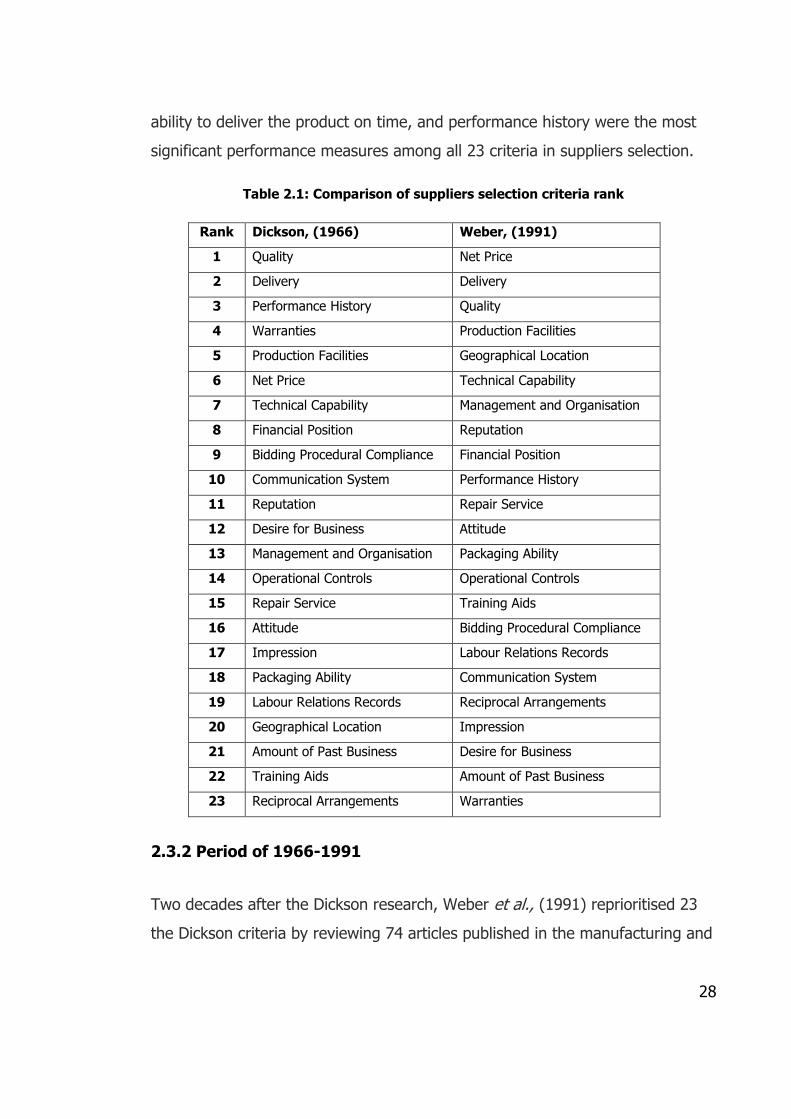
2.3.2 Period of 1966-1991 ..................................................................................................................... 28
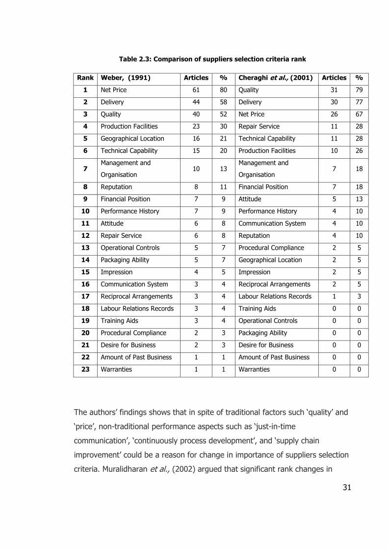
2.3.3 Period of 1991-2001 ..................................................................................................................... 30
2.3.4 Duration of 2001 to Present ......................................................................................................... 32
2.4 Suppliers Selection Methods ..........................................................................................................34
2.4.1 Individual Approaches .................................................................................................................. 35
Analytic Hierarchy Process (AHP) ......................................................................................... 36 2.4.1.1
Analytic Network Process (ANP) ........................................................................................... 37 2.4.1.2
Mathematical Programming (MP) ........................................................................................ 39 2.4.1.3
2.4.2 Integrated Approaches ................................................................................................................. 47
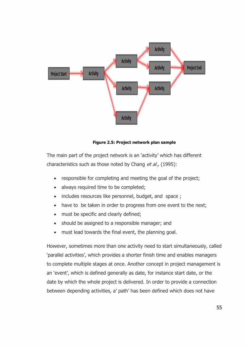
2.5 Project Management ......................................................................................................................52
2.5.1 Project Network Plan Development ............................................................................................. 54
2.6 Summary ........................................................................................................................................57
CHAPTER 3 DEVELOPMENT OF THE SUPPLIERS SELECTION FRAMEWORK
AND ALGORITHMS .............................................................................................................. 59
3.1 Introduction ...................................................................................................................................59
3.2 Contextual Considerations .............................................................................................................60
3.3 Suppliers Selection Framework Based on Cloud Manufacturing .....................................................61
3.3.1 Multi-Criteria Module ................................................................................................................... 63
Criteria Selection .................................................................................................................. 63 3.3.1.1
Criteria Normalisation .......................................................................................................... 63 3.3.1.2
Criteria Weighting ................................................................................................................. 65 3.3.1.3
3.3.2 Bidding Module ............................................................................................................................ 66
Request for Proposal (RFP) and Bids Management .............................................................. 67 3.3.2.1
Eligibility Screening ............................................................................................................... 68 3.3.2.2
Dominance Screening ........................................................................................................... 69 3.3.2.3
3.3.3 Optimisation Module ................................................................................................................... 69
Integrated Suppliers Selection and Project Time Planning ................................................... 70 3.3.3.1
3.3.4 Learning Module........................................................................................................................... 73
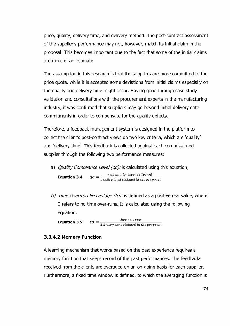
Feedback Management ........................................................................................................ 73 3.3.4.1
Memory Function ................................................................................................................. 74 3.3.4.2
Page 7
vii
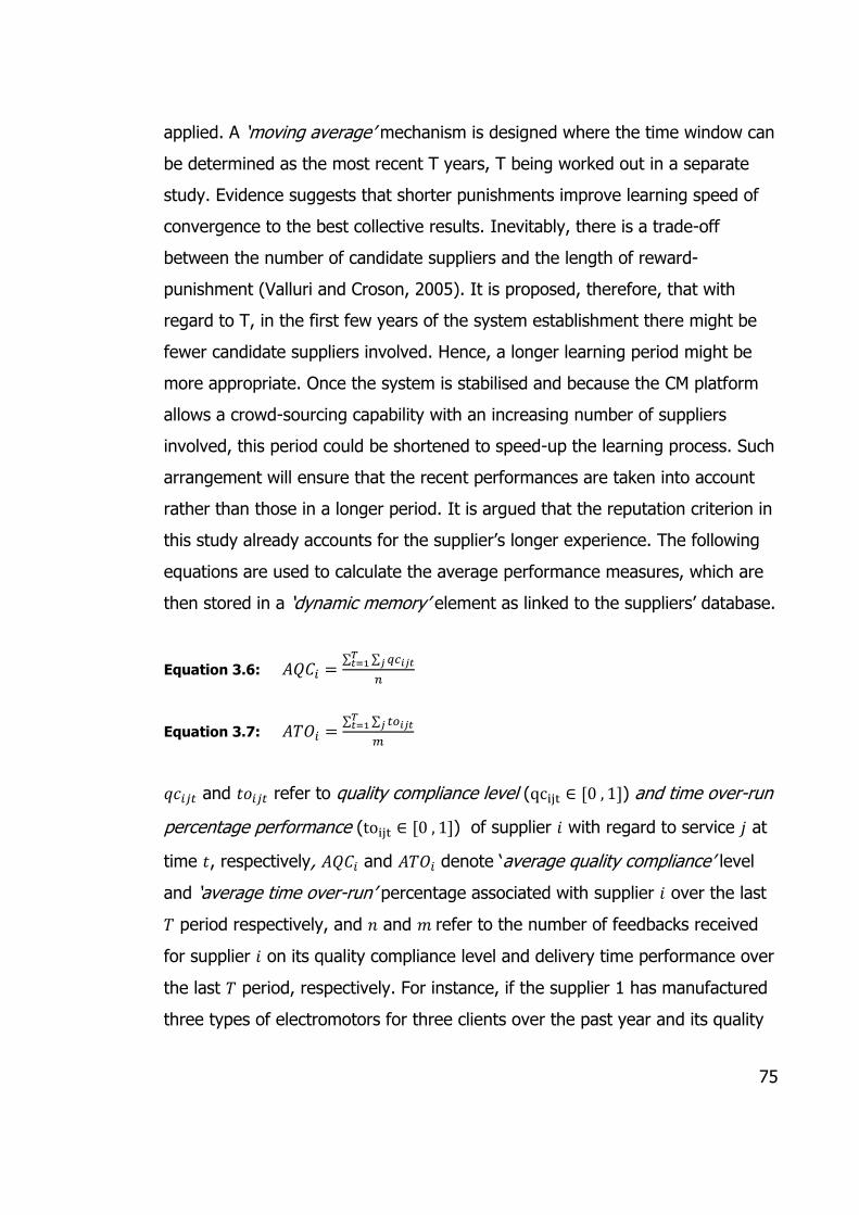
Learning Algorithm ............................................................................................................... 76 3.3.4.3
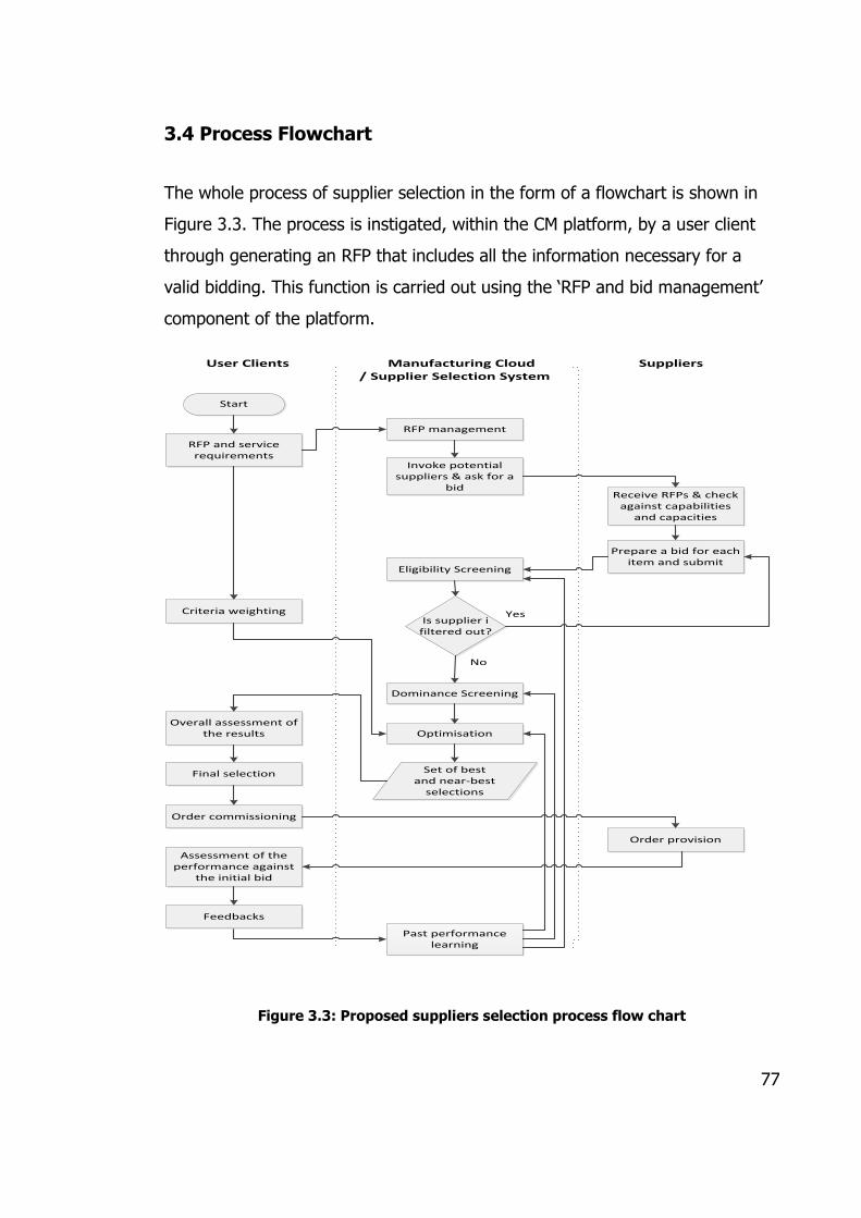
3.4 Process Flowchart ..........................................................................................................................77
3.5 Summary ........................................................................................................................................78
CHAPTER 4 FORMULATION OF THE SUPPLIERS SELECTION CRITERIA –
EXPERT OPINIONS SURVEY .............................................................................................. 81
4.1 Background and Theoretical Framework ........................................................................................81
4.1.1 Cost/Price ..................................................................................................................................... 83
4.1.2 Quality .......................................................................................................................................... 84
4.1.3 Delivery/Time ............................................................................................................................... 85
4.1.4 Reputation/Trust .......................................................................................................................... 86
4.2 Criteria Metrics ..............................................................................................................................87
4.3 Objective of the Survey ..................................................................................................................90
4.4 Participants ....................................................................................................................................90
4.5 Questionnaire Development ..........................................................................................................90
4.5.1 Piloting .......................................................................................................................................... 91
4.5.2 Implementation of the Survey ...................................................................................................... 91
4.5.3 Results and Analysis ..................................................................................................................... 92
4.5.4 Importance of Major Criteria Groups in Suppliers Selection ........................................................ 92
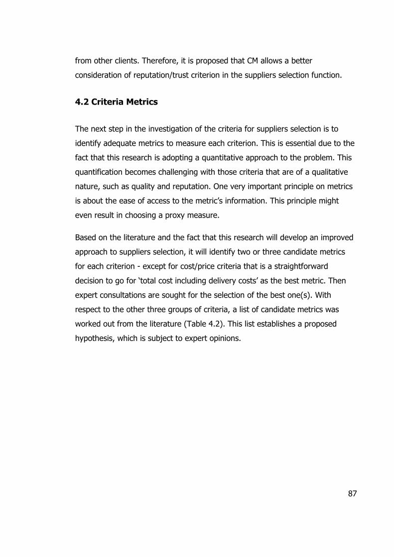
4.5.5 Metrics to Evaluate Criterion 'Quality of Service' ......................................................................... 93
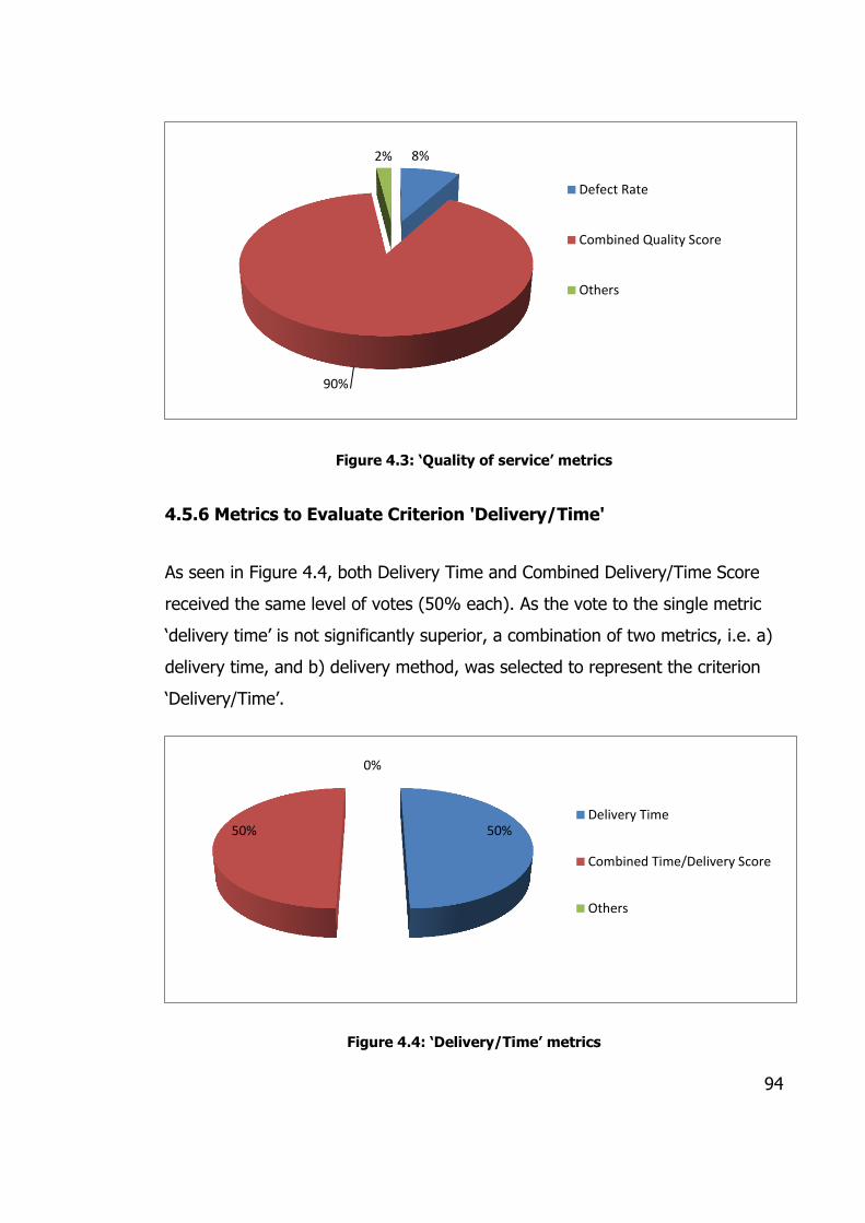
4.5.6 Metrics to Evaluate Criterion 'Delivery/Time' .............................................................................. 94
4.5.7 Criterion on 'Suppliers Reputation' .............................................................................................. 95
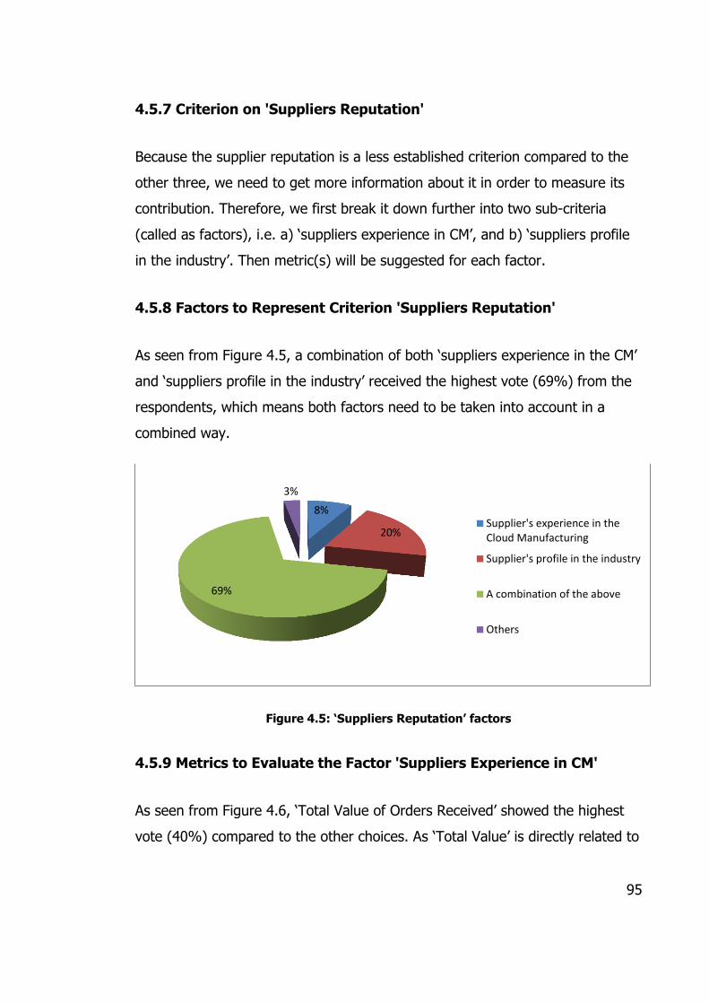
4.5.8 Factors to Represent Criterion 'Suppliers Reputation' ................................................................. 95
4.5.9 Metrics to Evaluate the Factor 'Suppliers Experience in CM' ....................................................... 95
4.5.10 Metrics to Evaluate the Factor 'Suppliers Profile in the Industry' .............................................. 96
4.5.11 Further Validation via Case Studies ............................................................................................ 97
4.5.12 Final Results ................................................................................................................................ 97
4.6 Summary ........................................................................................................................................98
Page 8
viii
CHAPTER 5 DEVELOPMENT OF THE OPTIMISATION-BASED MODELING ON
SUPPLIERS SELECTION FOR A SET OF SERVICES ...................................................... 99
5.1 Introduction ...................................................................................................................................99
5.2 Assumptions ................................................................................................................................. 100
5.3 Criteria Metrics Normalisation Re-visited ..................................................................................... 100
5.4 Mathematical Programming Model .............................................................................................. 103
5.5 Modelling of the Suppliers Selection Component ......................................................................... 104
5.5.1 Decision Variables ...................................................................................................................... 104
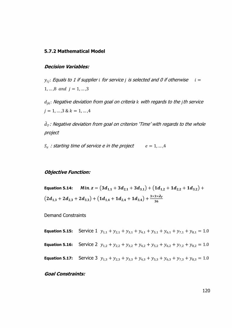
5.5.2 Objective Function...................................................................................................................... 107
5.5.3 Demand Constraints ................................................................................................................... 109
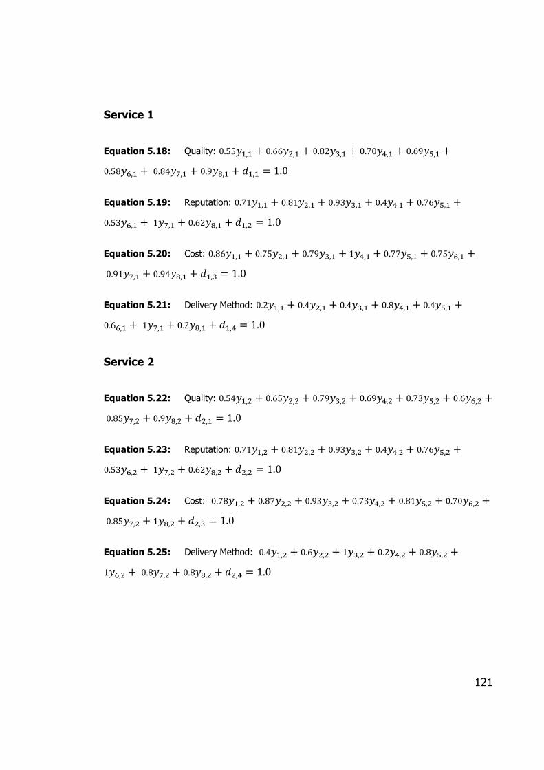
5.5.4 Goal Constraints ......................................................................................................................... 109
Quality Goal Constraints ..................................................................................................... 110 5.5.4.1
Reputation Goal Constraints ............................................................................................... 110 5.5.4.2
Cost Method Goal Constraints ............................................................................................ 110 5.5.4.3
Delivery Goal Constraints ................................................................................................... 111 5.5.4.4
Non-negativity and Variable Types ..................................................................................... 111 5.5.4.5
5.6 Modelling of the Project Planning Segment .................................................................................. 111
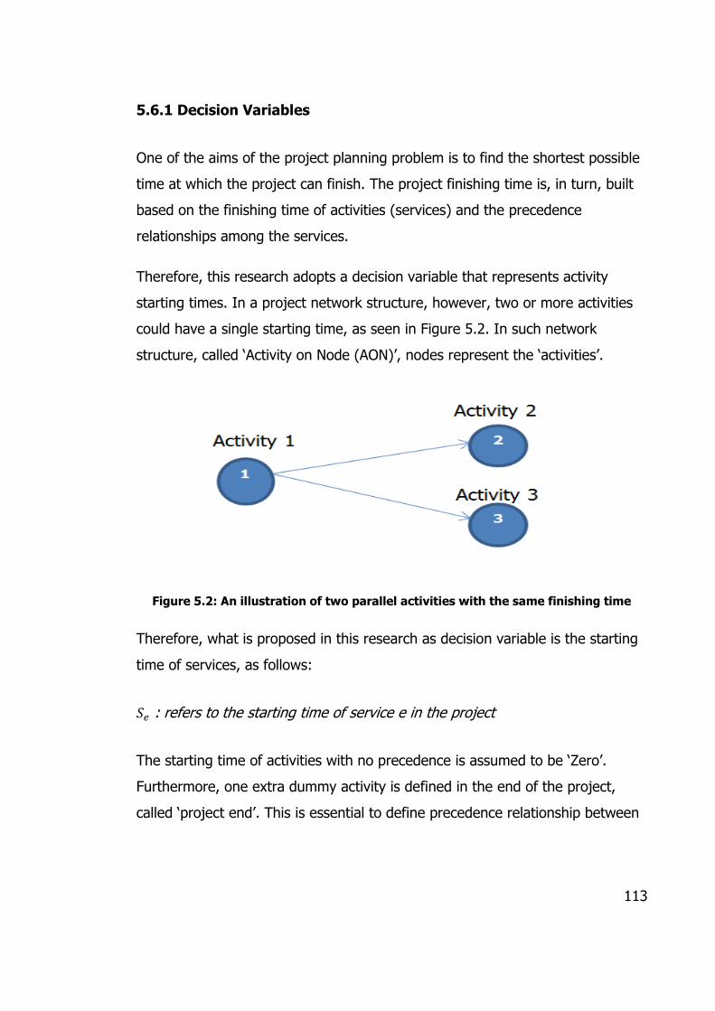
5.6.1 Decision Variables ...................................................................................................................... 113
5.6.2 Objective Function...................................................................................................................... 114
5.6.3 Constraints ................................................................................................................................. 114
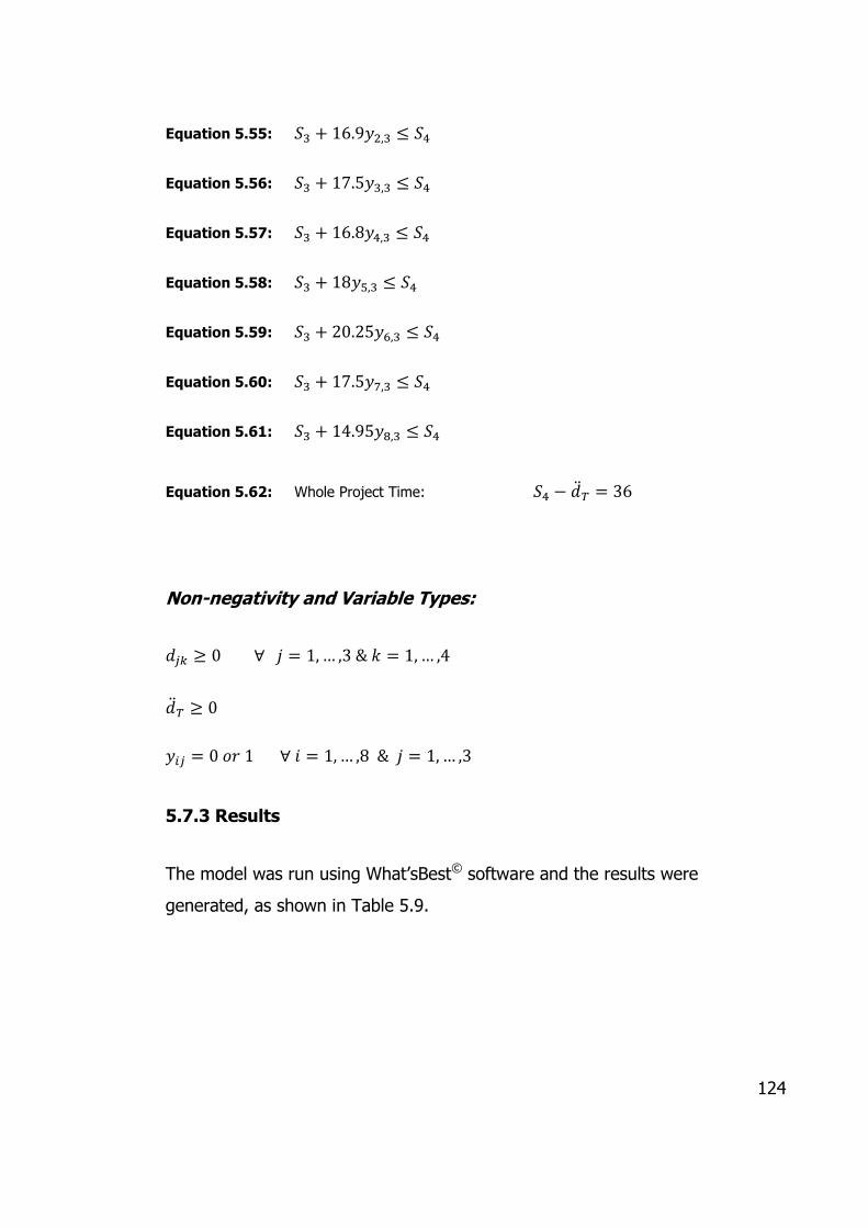
Project Planning Precedence Constraints ........................................................................... 114 5.6.3.1
Delivery Time Goal Constraint ............................................................................................ 115 5.6.3.2
5.6.4 Non-negativity ............................................................................................................................ 116
5.7 Numerical Example ...................................................................................................................... 116
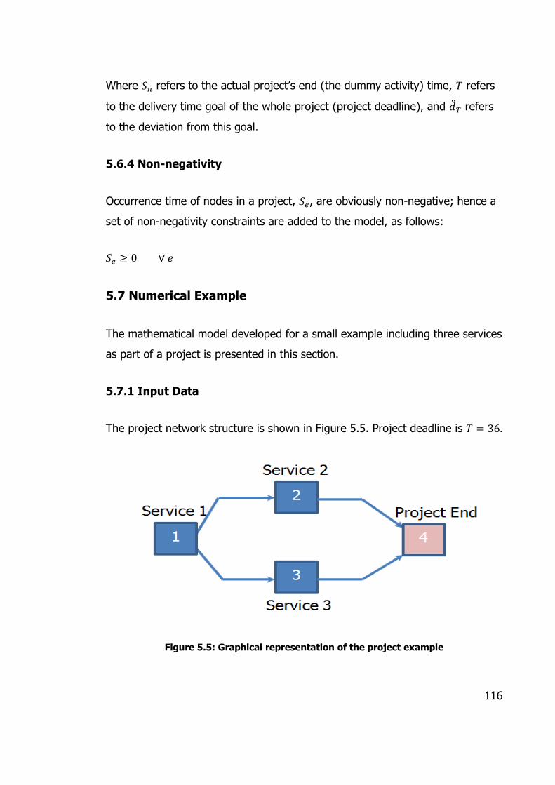
5.7.1 Input Data ................................................................................................................................... 116
5.7.2 Mathematical Model .................................................................................................................. 120
5.7.3 Results ........................................................................................................................................ 124
5.8 Summary ...................................................................................................................................... 125
Page 9
ix
CHAPTER 6 CASE STUDY IN THE OIL AND GAS INDUSTRY .................................. 127
6.1 Introduction ................................................................................................................................. 127
6.2 Case Study Setting ........................................................................................................................ 127
6.2.1 Objectives and Scope ................................................................................................................. 129
6.2.2 Recommendations on the Criteria ............................................................................................. 130
6.3 Services and Suppliers Proposals .................................................................................................. 130
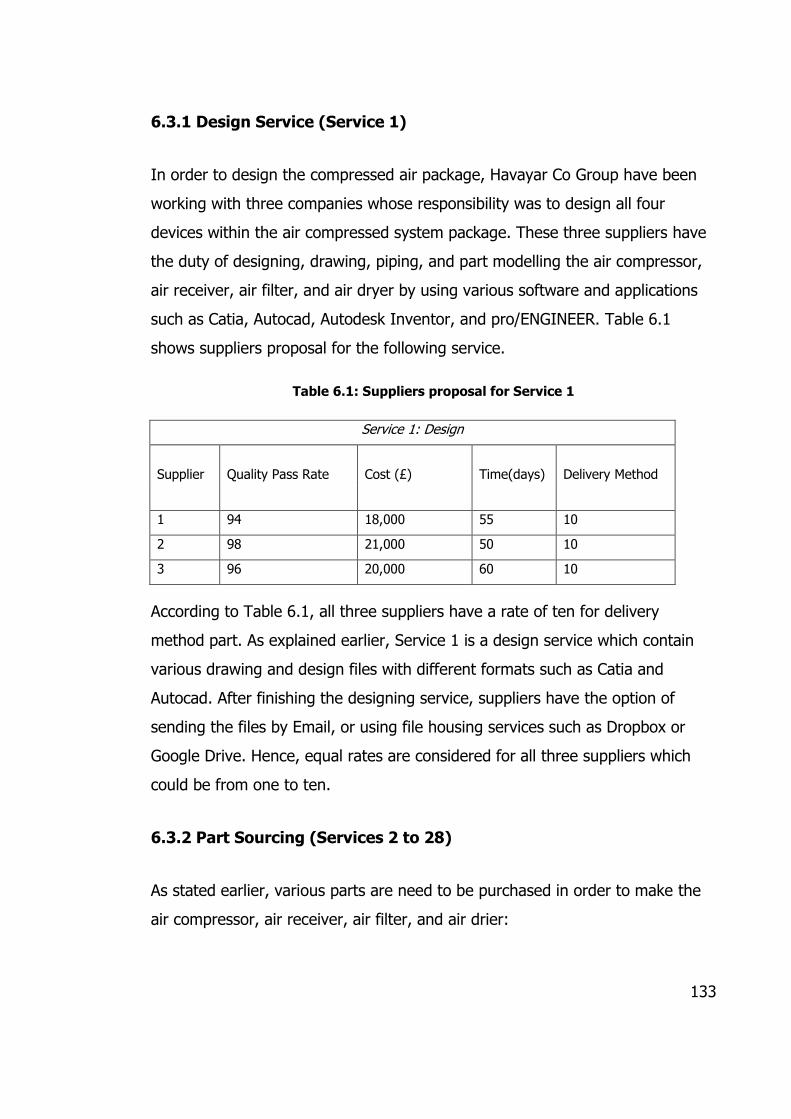
6.3.1 Design Service (Service 1) ........................................................................................................... 133
6.3.2 Part Sourcing (Services 2 to 28) .................................................................................................. 133
Air Compressor (Services 2 to 9) ......................................................................................... 134 6.3.2.1
Air Receiver (Services 10 to 15) .......................................................................................... 134 6.3.2.2
Air Filter (Services 16 and 17) ............................................................................................. 135 6.3.2.3
Air Drier (Services 18 and 28) ............................................................................................. 135 6.3.2.4
6.3.3 Transportation Service (Services 29) .......................................................................................... 136
6.4 Suppliers Information and Normalisation ..................................................................................... 136
6.4.1 Criteria Weighting ...................................................................................................................... 139
6.4.2 Normalisation ............................................................................................................................. 143
6.4.3 Suppliers Historical Dynamic Data .............................................................................................. 146
6.5 Project Time Planning and Precedence Relationships ................................................................... 148
6.6 Eligibility Screening ...................................................................................................................... 151
6.7 Dominance Screening ................................................................................................................... 152
6.8 Optimisation Model ..................................................................................................................... 152
6.8.1 Decision Variables ...................................................................................................................... 153
6.8.2 Objective Function...................................................................................................................... 153
6.8.3 Constraints ................................................................................................................................. 154
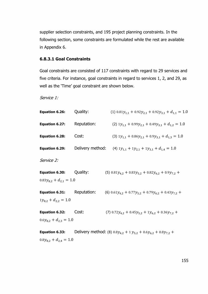
Goal Constraints ................................................................................................................. 155 6.8.3.1
Suppliers Selection Constraints .......................................................................................... 156 6.8.3.2
Project Planning Constraints ............................................................................................... 157 6.8.3.3
Non-negativity and Variable Types ..................................................................................... 159 6.8.3.4
6.9 Software Optimisation (What’sBest©
) and Final Results ............................................................... 159
Page 10
x
6.10 Analysis of Results ...................................................................................................................... 161
6.10.1 Sensitivity Analysis ................................................................................................................... 161
Quality - Scenario no.1 - (Quality weight=1) ..................................................................... 162 6.10.1.1
Cost ................................................................................................................................... 165 6.10.1.2
Reputation ........................................................................................................................ 167 6.10.1.3
Delivery Method ............................................................................................................... 169 6.10.1.4
Time .................................................................................................................................. 171 6.10.1.5
6.11 Summary .................................................................................................................................... 176
CHAPTER 7 CONCLUSIONS AND RECOMENDATIONS FOR FUTURE WORK.... 177
7.1 Overall Conclusions ...................................................................................................................... 177
7.2 Fulfilment of the Project Objectives ............................................................................................. 177
7.3 Research Contributions ................................................................................................................ 181
7.4 Recommendations for Future Work ............................................................................................. 182
References ........................................................................................................................... 184
Appendices ........................................................................................................................... 201
Appendix 1: Questionnaire ................................................................................................... 201
Appendix 2: Suppliers Proposals ........................................................................................... 208
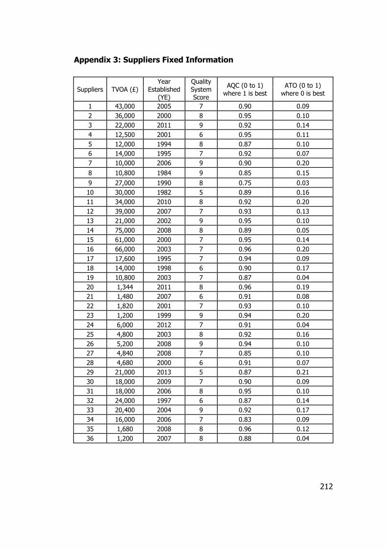
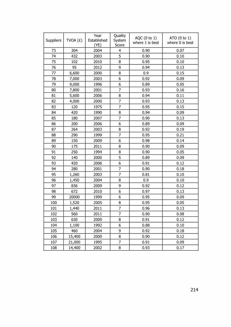
Appendix 3: Suppliers Fixed Information .............................................................................. 212
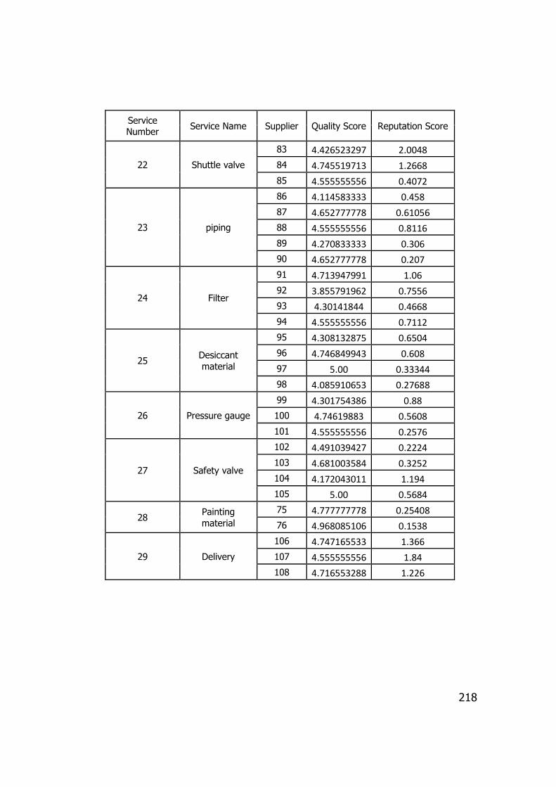
Appendix 4: Quality and Reputation Scores.......................................................................... 215
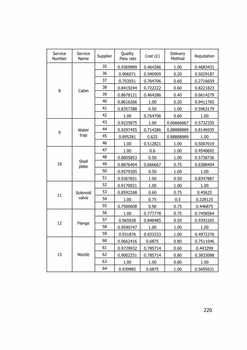
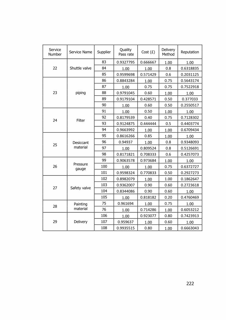
Appendix 5: Normalised Suppliers Proposals ....................................................................... 219
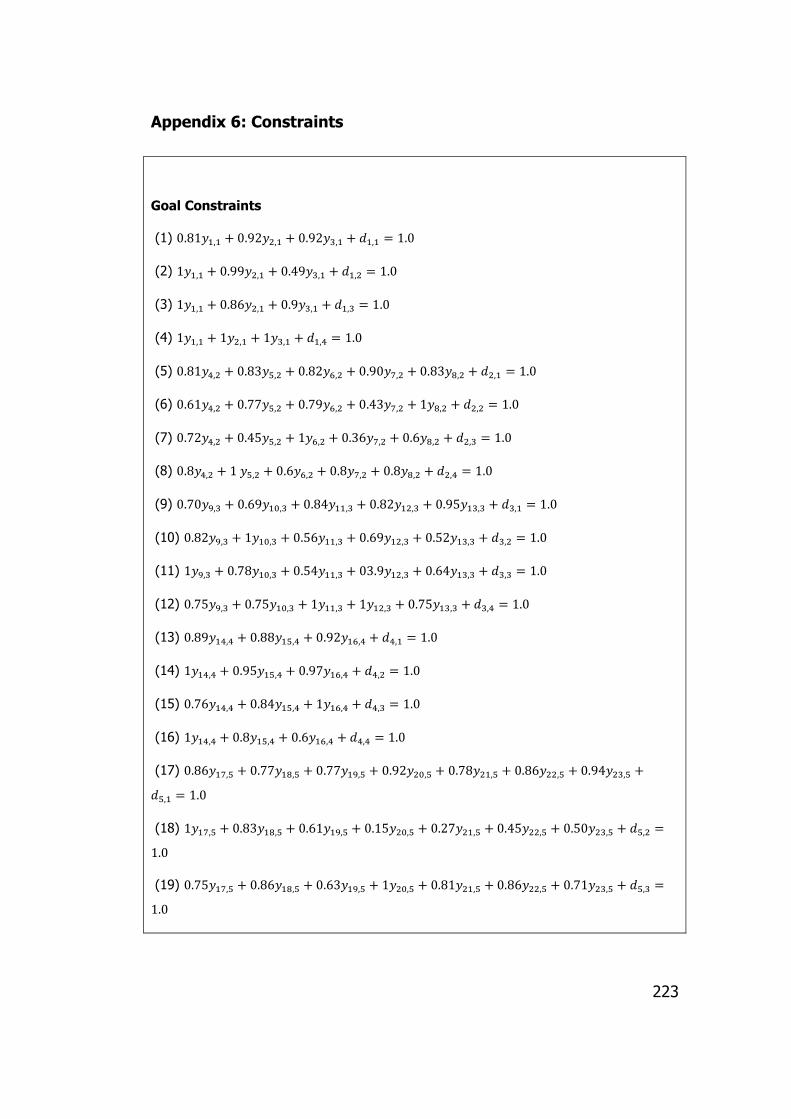
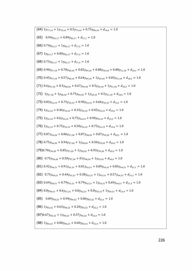
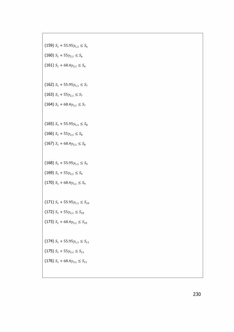
Appendix 6: Constraints ....................................................................................................... 223
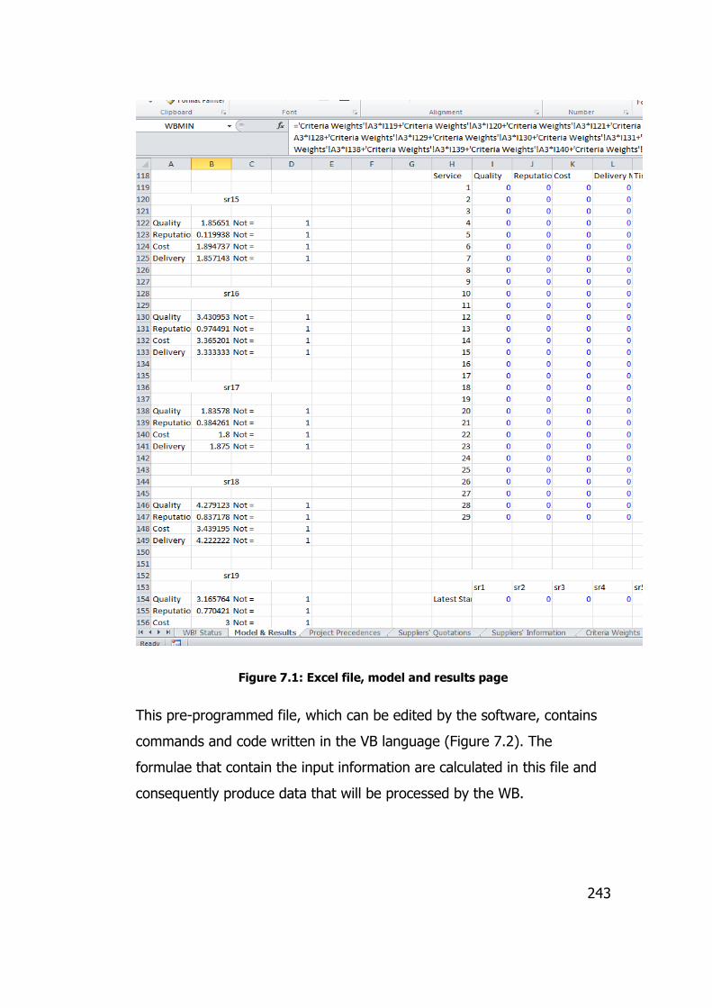
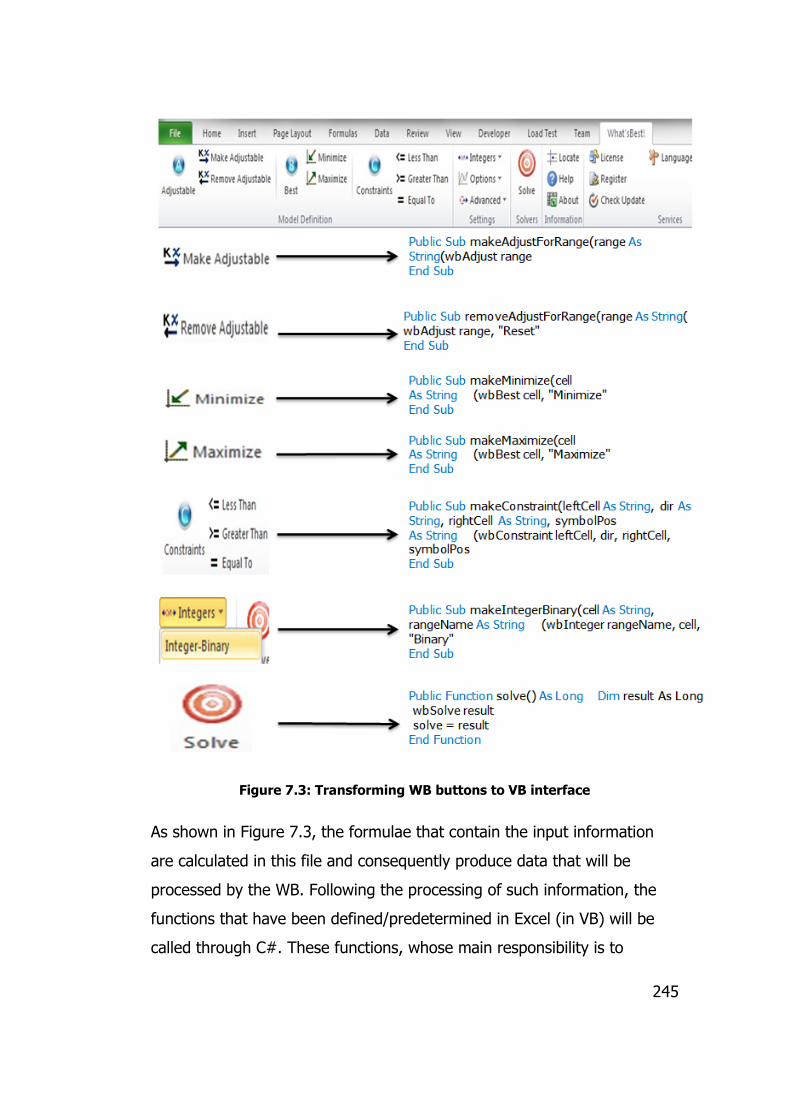
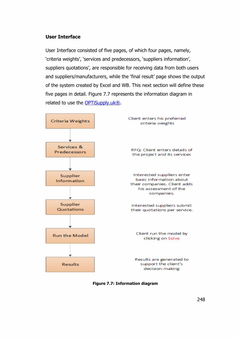
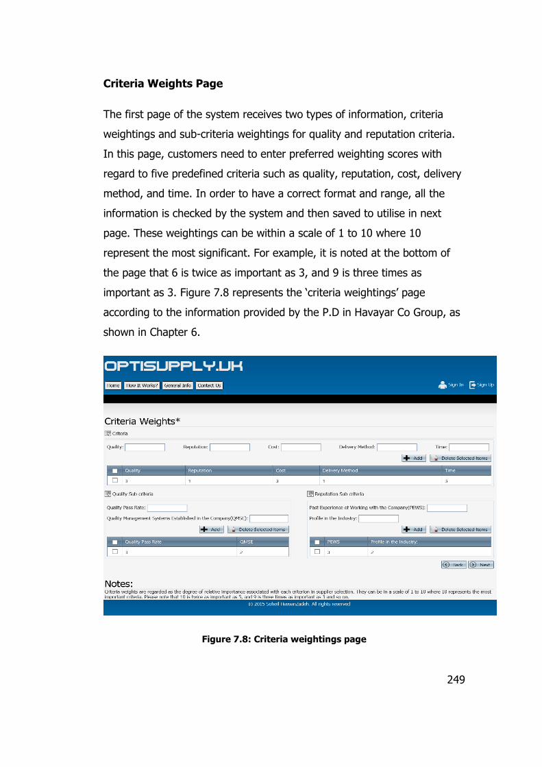
Appendix 7: System Development ........................................................................................ 240
Appendix 8: A List of Publications Arising from the PhD Research ........................................ 260
Page 11
xi
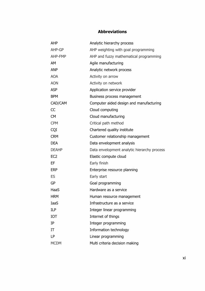
Abbreviations
AHP
AHP-GP
AHP-FMP
AM
ANP
AOA
AON
ASP
BPM
CAD/CAM
CC
CM
CPM
CQI
CRM
DEA
DEAHP
EC2
EF
ERP
ES
GP
HaaS
HRM
IaaS
ILP
IOT
IP
IT
LP
MCDM
Analytic hierarchy process
AHP weighting with goal programming
AHP and fuzzy mathematical programming
Agile manufacturing
Analytic network process
Activity on arrow
Activity on network
Application service provider
Business process management
Computer aided design and manufacturing
Cloud computing
Cloud manufacturing
Critical path method
Chartered quality institute
Customer relationship management
Data envelopment analysis
Data envelopment analytic hierarchy process
Elastic compute cloud
Early finish
Enterprise resource planning
Early start
Goal programming
Hardware as a service
Human resource management
Infrastructure as a service
Integer linear programming
Internet of things
Integer programming
Information technology
Linear programming
Multi criteria decision making
Page 12
xii
MGrid
MIGP
MILP
MP
NM
OR
PaaS
PD
PMI
QMSC
RFP
RSD
RSP
SAW
SaaS
SCM
SIP
SMEs
SOA
UFI
WB
Manufacturing grid
Mixed integer-goal programming
Mixed integer-linear programming
Mathematical programming
Networked manufacturing
Operation research
Platform as a service
Procurement department
Project management institute
Quality management system certifications
Request for proposal
Resource service demander
Resource service provider
Simple additive weighting
Software as a service
Supply chain management
Stochastic integer programming
Small and medium sized enterprises
Service-orientated architecture
User friendly interface
What’s best
Page 13
xiii
List of Figures
FIGURE 1.1: A TREND OF MANUFACTURING SYSTEMS DEVELOPMENT ...................................................... 3
FIGURE 1.2: MASS PRODUCTION AGAINST MASS CUSTOMISATION ........................................................... 5
FIGURE 1.3: MODERN SCM NETWORK ......................................................................................................... 7
FIGURE 1.4: CLOUD COMPUTING SERVICE MODELS .................................................................................. 12
FIGURE 1.5: THE FRAMEWORK AND MAIN LAYERS OF CLOUD MANUFACTURING ................................... 15
FIGURE 1.6: DIFFERENT NETWORK SEQUENCE IN PROJECT ...................................................................... 20
FIGURE 1.7: OVERVIEW OF THE THESIS STRUCTURE ................................................................................. 23
FIGURE 2.1: COMPARISON OF FACTORS (PERIOD OF 1966-1991 AND 1991-2001)................................... 32
FIGURE 2.2: ANP MODEL INSTANCE ........................................................................................................... 38
FIGURE 2.3: HIERARCHAL STRUCTURE (LEFT) AGAINST NETWORK STRUCTURE (RIGHT) .......................... 39
FIGURE 2.4: MATHEMATICAL PROGRAMMING DEVELOPMENT STAGES ................................................... 40
FIGURE 3.1: CLOUD MANUFACTURING SERVICES ...................................................................................... 61
FIGURE 3.2: PROPOSED SUPPLIERS SELECTION OPTIMISATION FRAMEWORK IN THE CONTEXT OF CM .. 62
FIGURE 3.3: PROPOSED SUPPLIERS SELECTION PROCESS FLOW CHART .................................................... 77
FIGURE 4.1: NUMBER OF RESPONDENTS BY CATEGORY ........................................................................... 92
FIGURE 4.2: IMPORTANCE OF MAJOR CRITERIA GROUPS IN SUPPLIERS SELECTION ................................. 93
FIGURE 4.3: ‘QUALITY OF SERVICE’ METRICS ............................................................................................. 94
FIGURE 4.4: ‘DELIVERY/TIME’ METRICS ..................................................................................................... 94
FIGURE 4.5: ‘SUPPLIERS REPUTATION’ FACTORS ....................................................................................... 95
FIGURE 4.6: ‘SUPPLIERS EXPERIENCE IN CM’ METRICS .............................................................................. 96
FIGURE 4.7: ‘SUPPLIERS PROFILE IN THE INDUSTRY’ METRICS .................................................................. 96
FIGURE 5.1: AN EXAMPLE OF A CLASSIC GRAPHICAL-BASED CPM ANALYSIS .......................................... 112
FIGURE 5.2: AN ILLUSTRATION OF TWO PARALLEL ACTIVITIES WITH THE SAME FINISHING TIME ......... 113
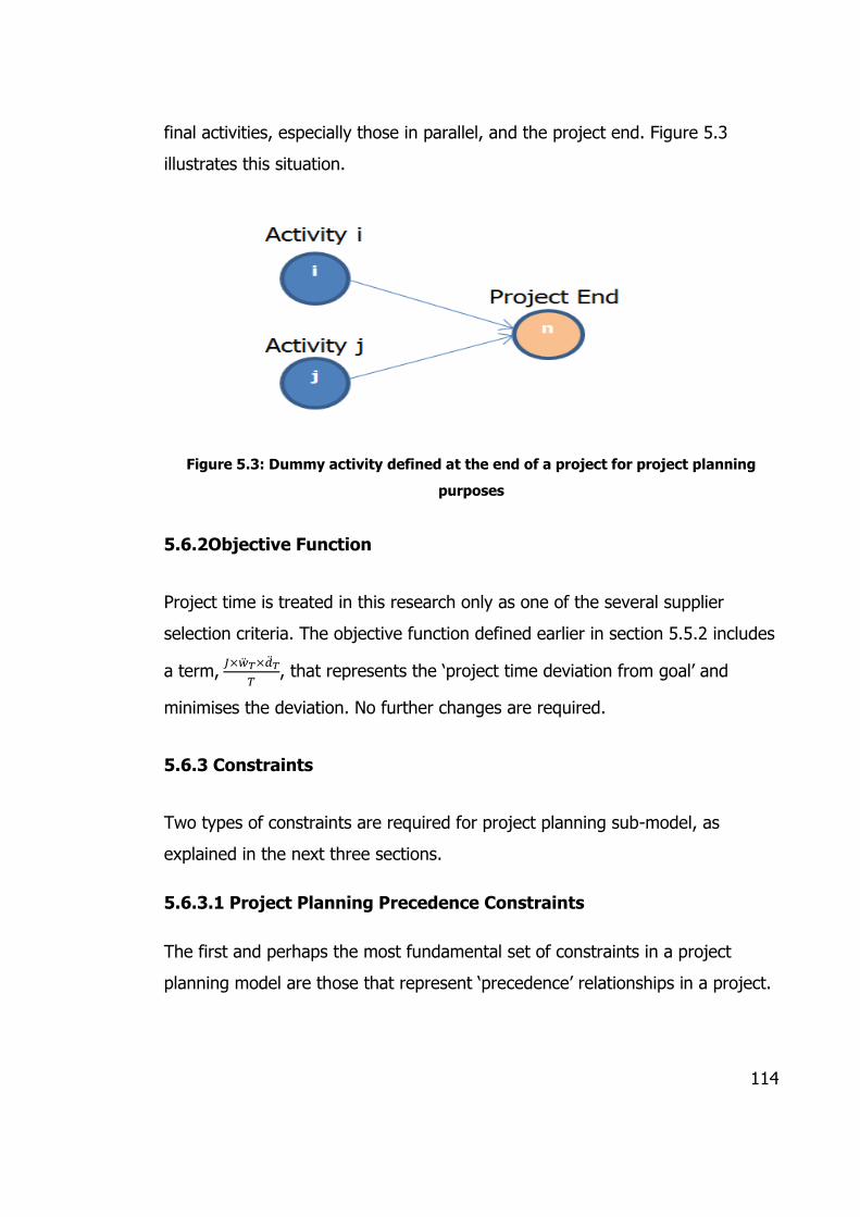
FIGURE 5.3: DUMMY ACTIVITY DEFINED AT THE END OF A PROJECT FOR PROJECT PLANNING PURPOSES
........................................................................................................................................................ 114
FIGURE 5.4: GRAPHICAL REPRESENTATION OF PRECEDENCE RELATIONSHIPS IN THIS RESEARCH ......... 115
FIGURE 5.5: GRAPHICAL REPRESENTATION OF THE PROJECT EXAMPLE ................................................. 116
FIGURE 6.1: THE GEOGRAPHICAL LOCATION OF THE PROJECT SIZE ........................................................ 128
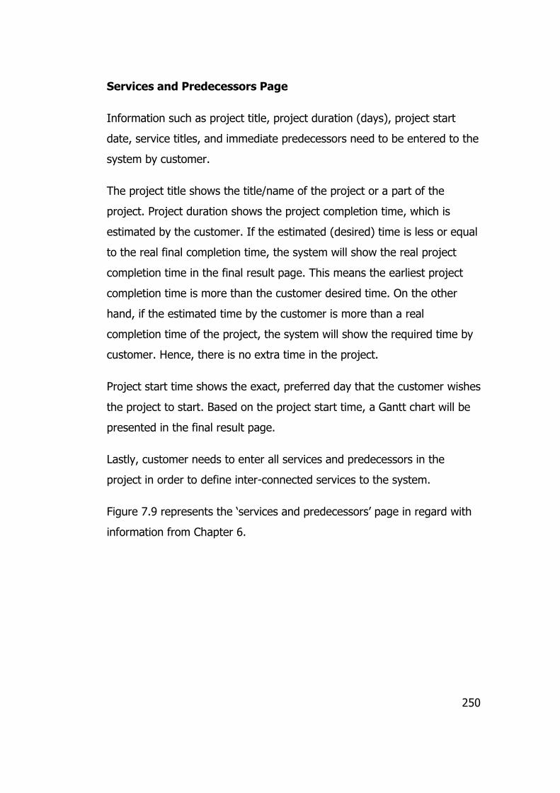
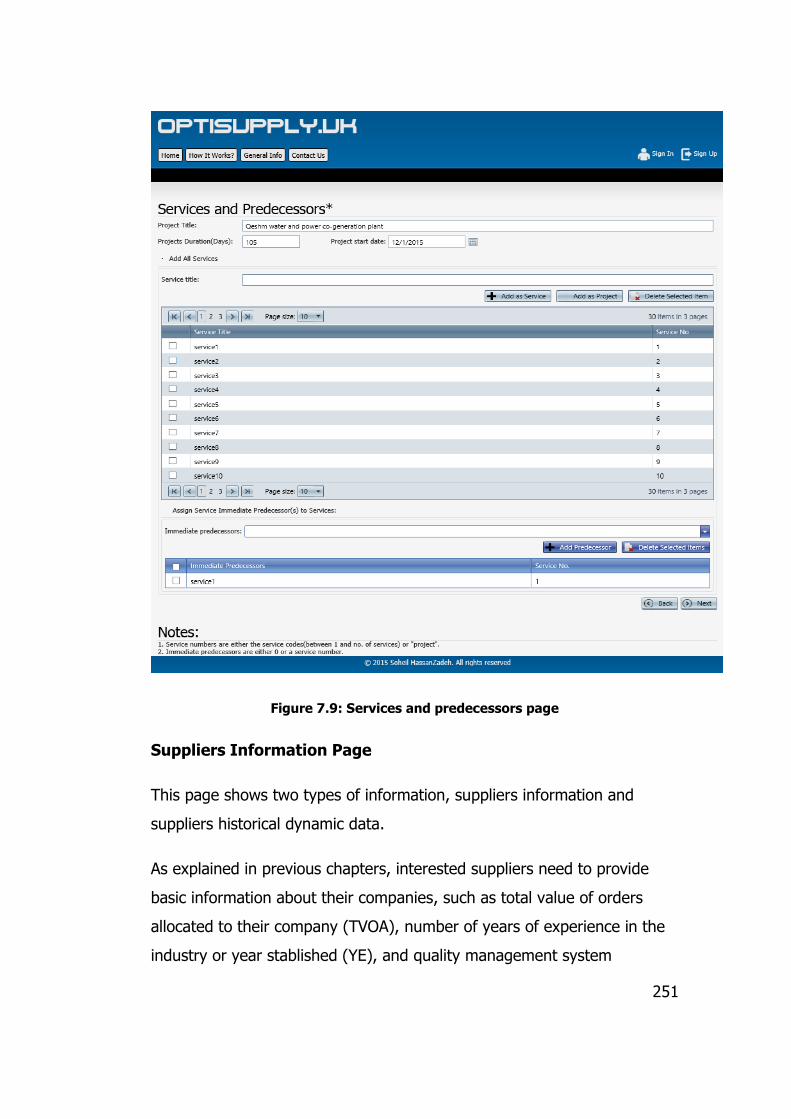
FIGURE 6.2: LIST OF ALL 29 SERVICES ASSOCIATED WITH THE PROJECT ................................................. 131
FIGURE 6.3: INTER-CONNECTED SERVICES AND PREDECESSORS ............................................................. 148
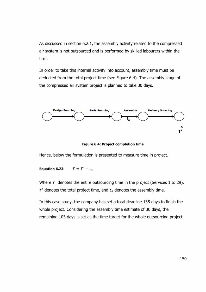
FIGURE 6.4: PROJECT COMPLETION TIME ................................................................................................ 150
FIGURE 6.5: DIFFERENT SCENARIO COMPARISON ................................................................................... 175
Page 14
xiv
List of Tables
TABLE 1.1: FEATURES OF EXISTING ADVANCED MANUFACTURING SYSTEMS ........................................... 13
TABLE 2.1: COMPARISON OF SUPPLIERS SELECTION CRITERIA RANK ........................................................ 28
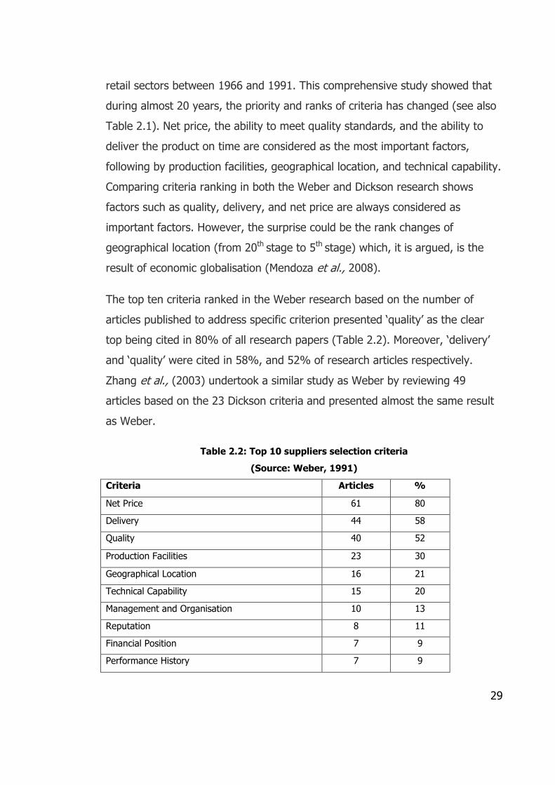
TABLE 2.2: TOP 10 SUPPLIERS SELECTION CRITERIA .................................................................................. 29
TABLE 2.3: COMPARISON OF SUPPLIERS SELECTION CRITERIA RANK ........................................................ 31
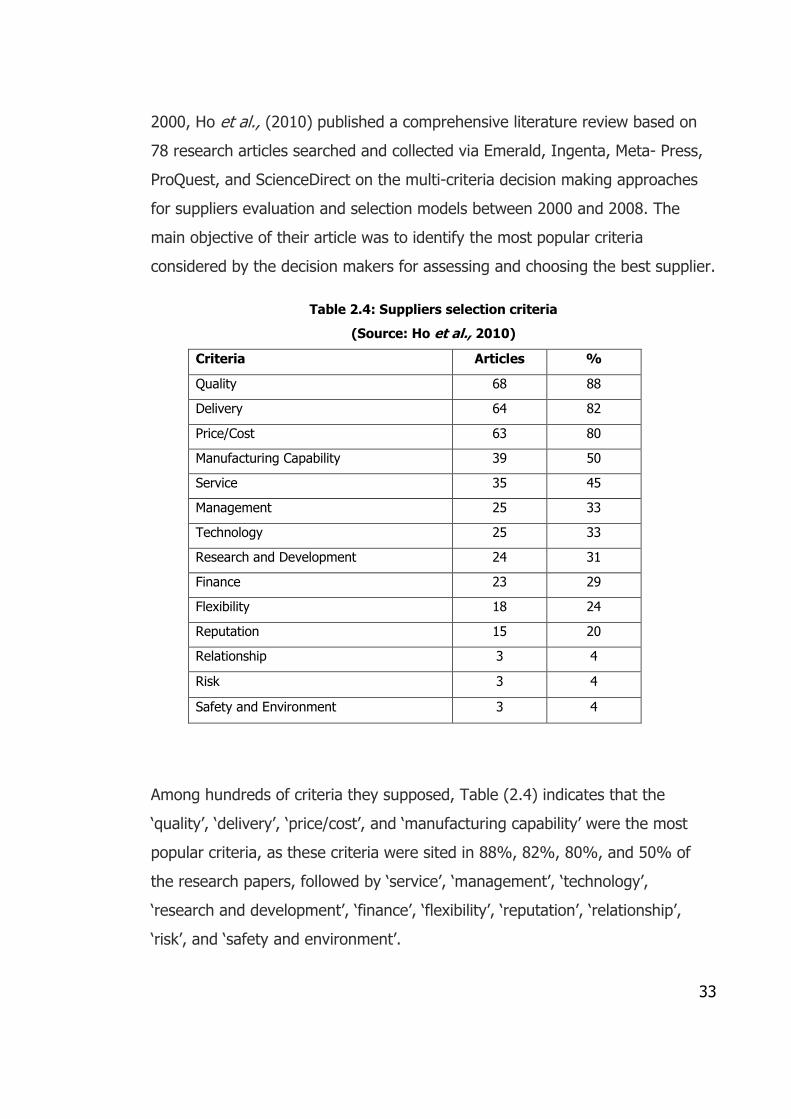
TABLE 2.4: SUPPLIERS SELECTION CRITERIA ............................................................................................... 33
TABLE 2.5: COMPARISON OF DIFFERENT DECISION-MAKING METHODS .................................................. 51
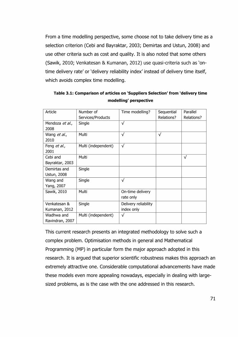
TABLE 3.1: COMPARISON OF ARTICLES ON ‘SUPPLIERS SELECTION’ FROM ‘DELIVERY TIME MODELLING’
PERSPECTIVE ..................................................................................................................................... 71
TABLE 4.1: CRITERIA FOR SUPPLIERS SELECTION CITED IN THE LITERATURE ............................................. 82
TABLE 4.2: PRELIMINARY LIST OF CANDIDATE METRICS AND THEIR DESCRIPTIONS ................................. 88
TABLE 4.3: FINAL LIST OF METRICS ............................................................................................................ 97
TABLE 5.1: FINAL LIST OF METRICS .......................................................................................................... 101
TABLE 5.2: STANDARD FORM OF A MATHEMATICAL MODEL .................................................................. 104
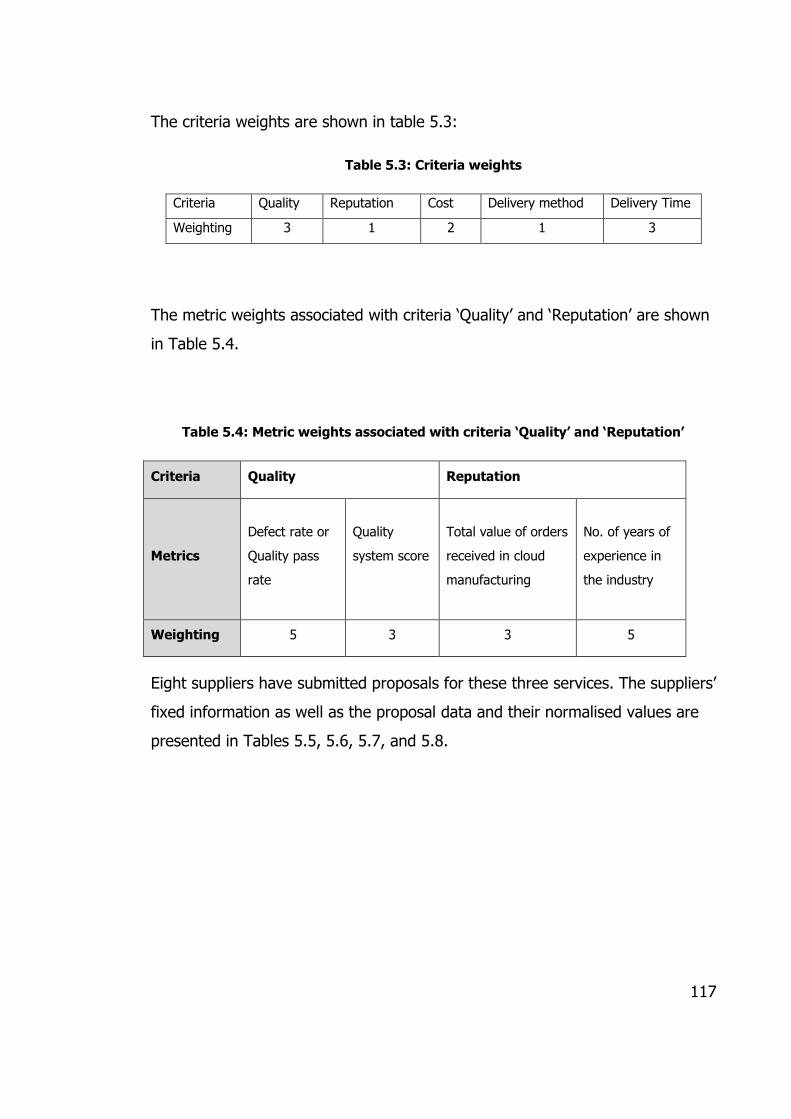
TABLE 5.3: CRITERIA WEIGHTS ................................................................................................................. 117
TABLE 5.4: METRIC WEIGHTS ASSOCIATED WITH CRITERIA ‘QUALITY’ AND ‘REPUTATION’ ................... 117
TABLE 5.5: SUPPLIERS FIXED INFORMATION............................................................................................ 118
TABLE 5.6: SUPPLIERS PROPOSALS (SERVICE1) ........................................................................................ 118
TABLE 5.7: SUPPLIERS PROPOSALS (SERVICE2) ........................................................................................ 119
TABLE 5.8: SUPPLIERS PROPOSALS (SERVICE3) ........................................................................................ 119
TABLE 5.9: MODEL RESULTS FOR THE NUMERICAL EXAMPLE ................................................................. 125
TABLE 6.1: SUPPLIERS PROPOSAL FOR SERVICE 1 .................................................................................... 133
TABLE 6.2: SUPPLIERS PROPOSAL FOR SERVICE 2 .................................................................................... 134
TABLE 6.3: SUPPLIERS PROPOSAL FOR SERVICE 10 .................................................................................. 135
TABLE 6.4: SUPPLIERS PROPOSAL FOR SERVICE 16 AND SERVICE 17 ....................................................... 135
TABLE 6.5: SUPPLIERS PROPOSAL FOR SERVICE 29 .................................................................................. 136
TABLE 6.6: SUPPLIERS PROFILE INFORMATION FOR SERVICES 1 TO 5 ..................................................... 138
TABLE 6.7: PREFERRED CRITERIA AND SUB-CRITERIA WEIGHTS PROPOSED BY PD ................................. 139
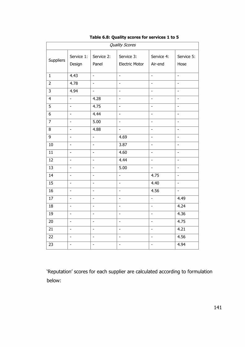
TABLE 6.8: QUALITY SCORES FOR SERVICES 1 TO 5 ................................................................................. 141
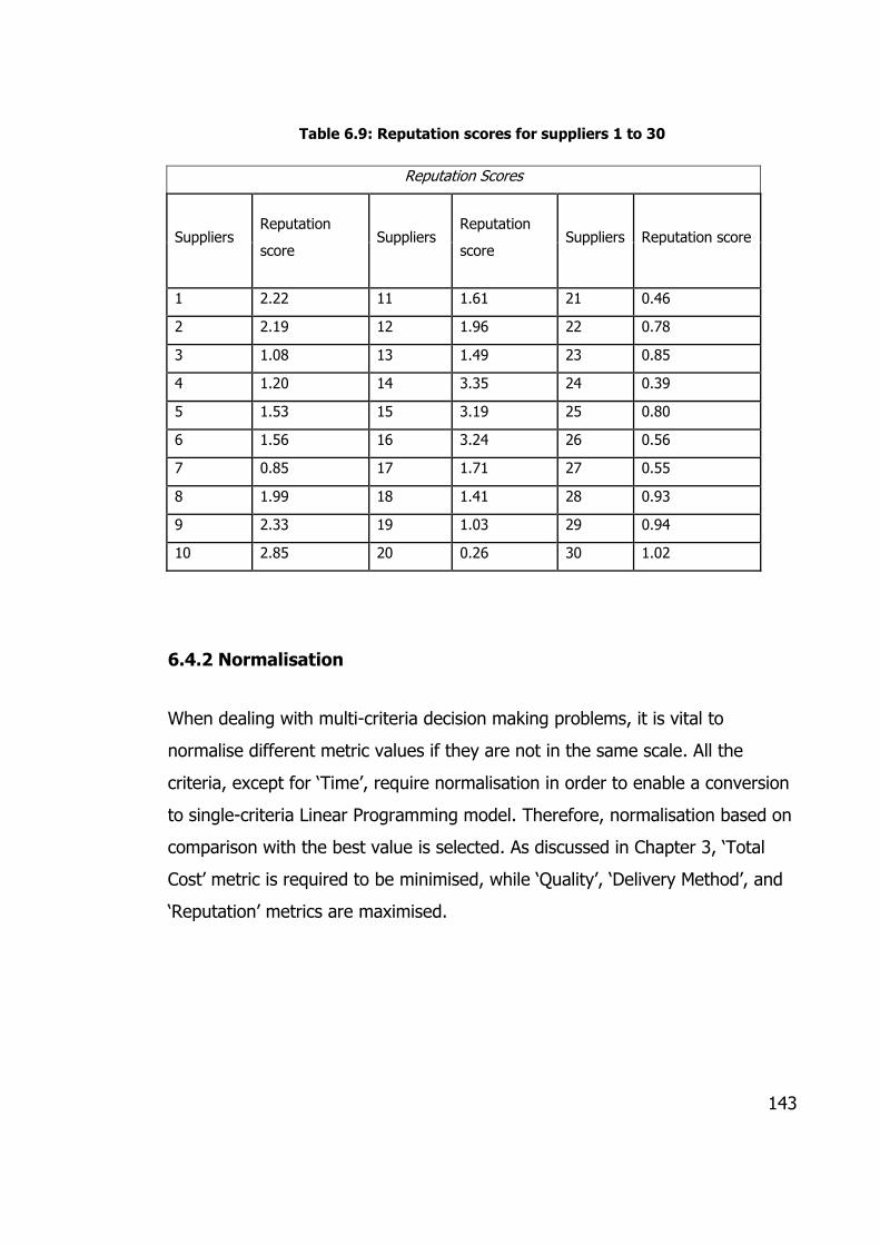
TABLE 6.9: REPUTATION SCORES FOR SUPPLIERS 1 TO 30 ...................................................................... 143
TABLE 6.10: SERVICE 1 (DESIGN) BEFORE AND AFTER NORMALISATION ................................................ 146
TABLE 6.11: SUPPLIERS HISTORICAL DYNAMIC DATA FOR SERVICE 1 TO 5 ............................................. 147
TABLE 6.12: PRECEDENCE RELATIONSHIPS BETWEEN SERVICES IN THE PROJECT ................................... 149
TABLE 6.13: SUPPLIERS PROPOSALS FILTERED OUT AS A RESULT OF ‘ELIGIBILITY SCREENING’ .............. 151
Page 15
xv
TABLE 6.14: SUPPLIERS PROPOSALS FILTERED OUT AS A RESULT OF ‘DOMINANCE SCREENING’ ........... 152
TABLE 6.15: FINAL RESULTS IN REGARD TO THE BASELINE SCENARIO .................................................... 160
TABLE 6.16: QUALITY WEIGHT =1 ............................................................................................................ 162
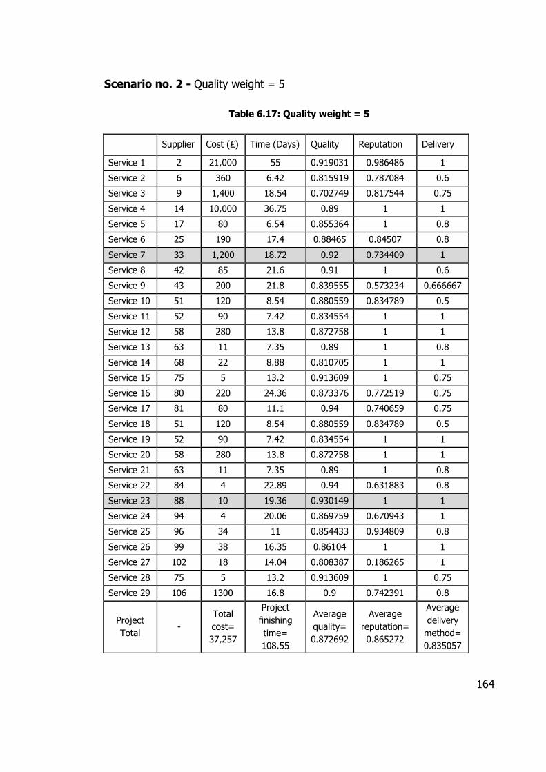
TABLE 6.17: QUALITY WEIGHT = 5 ............................................................................................................ 164
TABLE 6.18: COST WEIGHT = 1 ................................................................................................................. 166
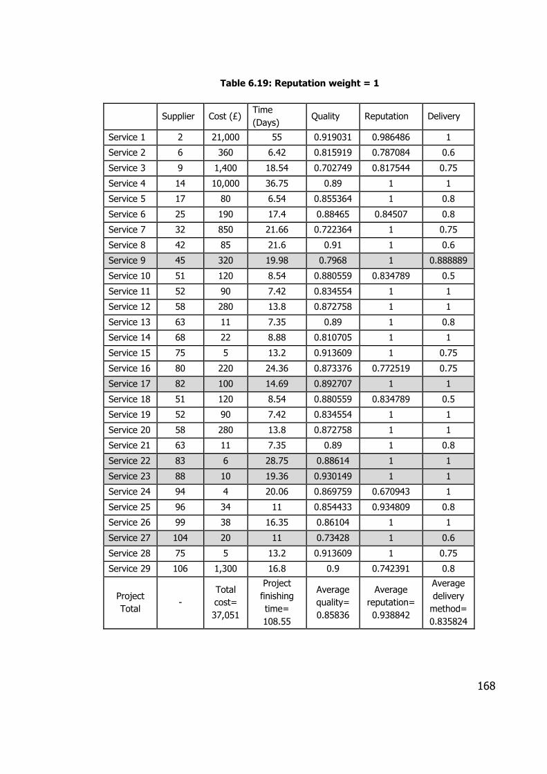
TABLE 6.19: REPUTATION WEIGHT = 1..................................................................................................... 168
TABLE 6.20: DELIVERY METHOD WEIGHT = 3 ........................................................................................... 170
TABLE 6.21: TIME WEIGHT = 1 ................................................................................................................. 172
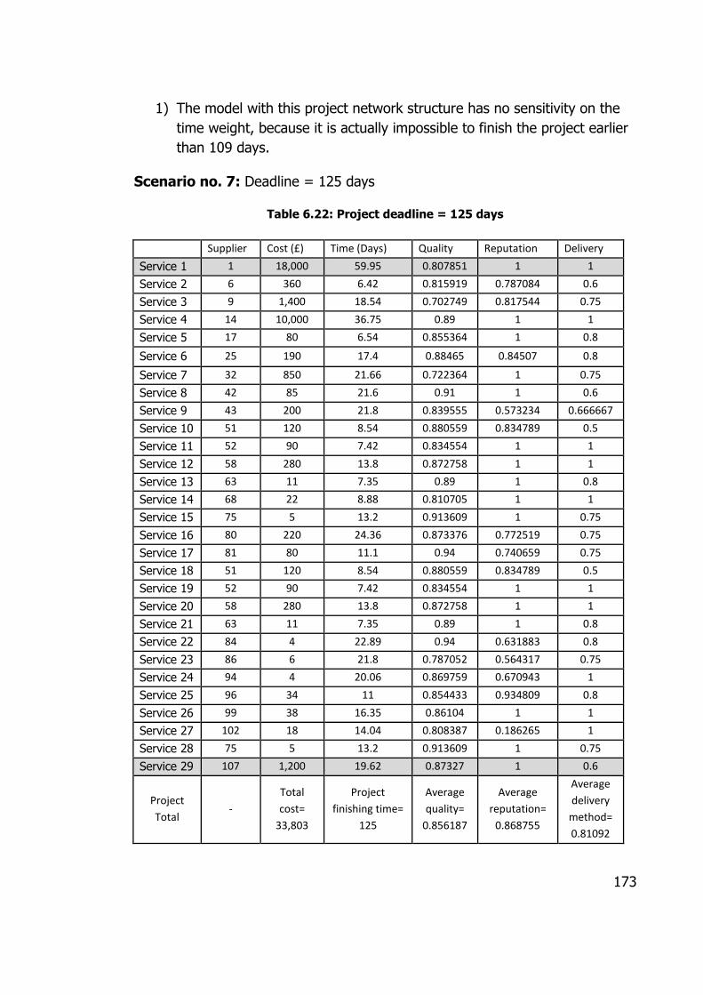
TABLE 6.22: PROJECT DEADLINE = 125 DAYS ........................................................................................... 173
Page 16
1
CHAPTER 1 INTRODUCTION
1.1 Introduction
Nowadays, the trend of globalisation is a great motivation for small and
medium sized enterprises (SMEs) worldwide. Many companies have decided to
use other companies’ competencies and outsource part of their manufacturing
and business processes to suppliers from abroad in order to reduce costs,
improve quality of products, and offer better services to customers. On the
other hand, this decision has faced organisations with new challenges.
Organisations need to evaluate their supplier’s performance, and consider their
weakness and strength to survive in high competitive markets. Hence, suppliers
evaluation and selection acts as an important strategy within enterprises.
The thesis is titled ‘a cloud manufacturing based approach to suppliers selection
and its implementation and application perspectives’. The suppliers section is
one of the main concepts of this research, which is considered as a
procurement strategy in the supply chain management (SCM) network. This
network facilitates a close relationship among enterprises, people, new
technologies, information, and various activities in order to deliver products
(both goods and services) to final customers.
In addition, Internet and new computing technologies provides a better
collaboration between customer, manufacturers, and suppliers. There are many
studies about the influence of Internet on marketing and sales. However, there
is a paucity of studies considering the role of novel technologies such as
Internet, intranet, and cloud technologies on manufacturing supply chain,
especially on selecting the most appropriate suppliers in whole SCM network.
This chapter includes seven sections. In Section 1.2, the historical trend of the
emergence of cloud manufacturing (CM) and the key concepts, such as, SCM,
Page 17
2
agile manufacturing (AM), manufacturing grid (MGrid), networked
manufacturing (NM), cloud computing (CC) and the analysis of all mentioned
approaches will be discussed. In Section 1.3, CM, and its advantages and
challenges will be discussed. To complete the chapter, motivations, aims and
objectives, the scope of the thesis, and the overview of the thesis structure are
presented.
1.2 Advances in Manufacturing Systems and Operations
Nowadays, manufacturing enterprises, especially SMEs, are faced with issues
such as different ranges of services, innovation, and fast changing customer
requirements, and, to deal with these, ‘agility’ is used as one of the main
factors to survive in highly competitive, manufacturing markets. In order to
cope with these issues and respond to new manufacturing requirements,
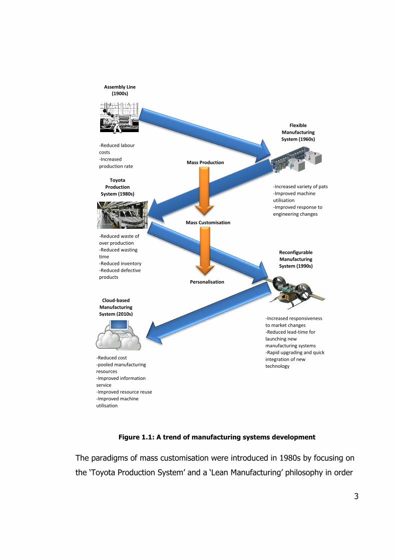
existing advanced manufacturing models require to be improved. Figure 1.1
shows the development of the manufacturing paradigms from mass production
to CM. According to customer requirements, manufacturing paradigms have
evolved through various approaches since the 1900s (Hu et al., 2011). Mass
production inspiring by ‘craft production’ is a model with low-cost products
through large scale manufacturing. Mass production had been introduced by
Henry Ford in the USA and adopted widely by other countries after Second
World War. Mass production was enabled by various concepts such as
interchangeability, moving assembly, and scientific management. Although
mass production enables customer to purchase their desirable product in an
affordable prices, limit production variety could not provide all of the customer
requirements. In other words, different ranges of customer requirements were
not included. High inventory costs were another main problem that faced
enterprises, especially when considering the number of unsold products left on
stock shelves.
Page 18
3
Figure 1.1: A trend of manufacturing systems development
The paradigms of mass customisation were introduced in 1980s by focusing on
the ‘Toyota Production System’ and a ‘Lean Manufacturing’ philosophy in order
Assembly Line (1900s)
-Reduced labour
costs
-Increased
production rate
Flexible
Manufacturing
System (1960s)
-Increased variety of pats -Improved machine
utilisation
-Improved response to
engineering changes
Toyota
Production
System (1980s)
Reconfigurable
Manufacturing
System (1990s)
Cloud-based
Manufacturing
System (2010s)
-Reduced waste of
over production
-Reduced wasting
time
-Reduced inventory
-Reduced defective
products
-Increased responsiveness
to market changes
-Reduced lead-time for
launching new
manufacturing systems
-Rapid upgrading and quick
integration of new
technology
-Reduced cost
-pooled manufacturing
resources
-Improved information
service
-Improved resource reuse
-Improved machine
utilisation
Mass Production
Mass Customisation
Personalisation
Page 19
4
to reduce inventory, minimise defective products, and diminish the waste of
over production (Pine II, 1993). As a result, variety and customisation through
flexibility and responsiveness has increased considerably. Hence, loyalty from
closer connection with the final user has grown while high supply chain costs
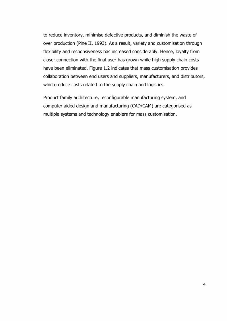
have been eliminated. Figure 1.2 indicates that mass customisation provides
collaboration between end users and suppliers, manufacturers, and distributors,
which reduce costs related to the supply chain and logistics.
Product family architecture, reconfigurable manufacturing system, and
computer aided design and manufacturing (CAD/CAM) are categorised as
multiple systems and technology enablers for mass customisation.
Page 20
5
Figure 1.2: Mass production against mass customisation
Hu et al., (2008) argued that high product variety has enabled enterprises to
meet customer demands, however, it had a direct influence on production
performance due to causing a complexity in the assembly systems. In addition,
the advent and widespread use of the Internet and computing has produced
positive results in the highly competitive market worldwide in recent years.
Innovation in products and more collaboration between manufacturers and end
users have shifted manufacturing paradigms through personalisation.
Moreover, one of the supportive concepts for realising the novel manufacturing
Mass Production
Mass Customisation
Deliver Purchase Make Source
Deliver Purchase Make Source
One way interaction
Two ways interaction
Traditional production model, where customer has no active role
Mass customisation, where customer takes active role
Self Service
Interaction
Page 21
6
paradigms is to realise and share manufacturing resources. In fact, the key to
improve the existing manufacturing models is to exploit fully all kinds of
potential manufacturing resources and capabilities (Hassanzadeh and Cheng,
2013). Hence, concepts such as SCM, AM, MGrid and, NM have emerged to face
the new challenges and evolved to optimise traditional methods.
1.2.1 Supply Chain Management
Collaborative relationship and shared-resource utilisation offered by various
enterprises help SMEs to deal with resource allocation issues. Collaborative
relationships between enterprises enable SMEs not only to have innovation in
process improvement, and product and technology development, but also to
provide better knowledge exchange between different organisations around the
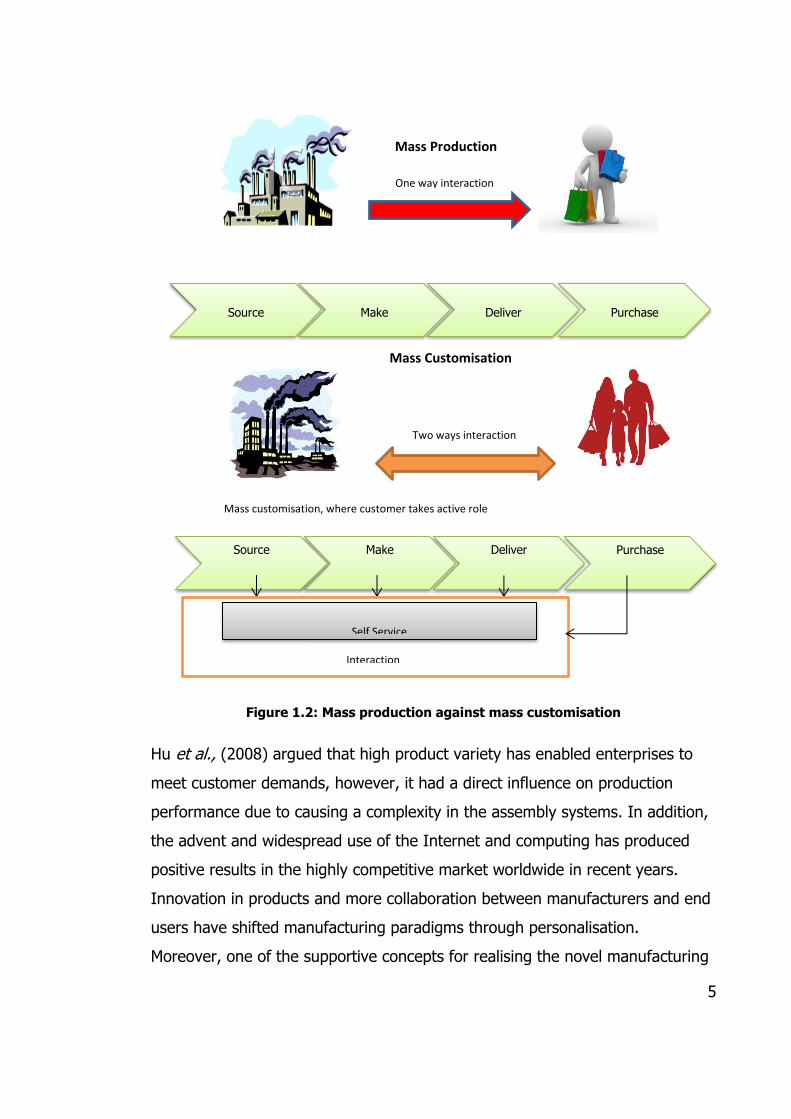
globe (Choi and Hong, 2002). Hence, the supply chain can become an
independent, intermediate type of network to connect enterprises, including
manufacturers, transporters, warehouses, and retailers, where supplies both
goods and services (see Figure 1.3).
Page 22
7
Figure 1.3: Modern SCM network
Figure 1.3 indicates that the product delivered through the supply chain is not
limited only to manufactured goods. The supply chain is also involved in the
distribution of services and knowledge/ information. While product flow has
only a one way relationship between functional entities starting from suppliers
and finishing by final customers, knowledge/ information flow is considered as a
two-way relationship among all four functional entities. Although the term of
SCM, stated by Oliver and Webbr (1982), in order to apply and promote
integrated business strategies in 1980s, SCM has been used widely and became
more popular after 2000s and has been adopted as an important approach in
business and production strategies.
SCM is a systematic and strategic management network allowing different kinds
of enterprise demands, including both tangible goods and services, in order to
improve enterprise long term strategies and performance. Apart from different
Product
Knowledge/Information
Supplier Manufacturer Distributer Customer
Page 23
8
definitions of SCM, many researchers believed that SCM would be more
operational when considered as a global network, not just a local network.
Hence, the term ‘global supply chain’ has emerged recently. Global supply chain
not only offers SMEs the ability to participate in a widespread geographical
variety of markets, but also provides a well-organised business, by improving
competitive advantages, time to market, inventory control, reputation and trust.
In addition, SMEs need to have an intelligent procurement strategy to reduce
their raw materials or purchasing costs. Consequently, SMEs have an
opportunity to bring lower cost products to market, which bring a competitive
advantage and better profits. Weber et al., (1991) stated that up to almost
80% of final product costs in manufacturing industries is because of material
and services purchasing costs. As shown in Figure 1.4, suppliers are indicated
as a beginning element of the whole SCM network, which have a great impact
on other elements in network. In fact, an enterprise could not be successful
and survive in a fierce competitive market unless they have an appropriate set
of suppliers as a key function in SCM.
1.2.2 Agile Manufacturing
In the 1980s, industry leaders popularised the terms of ‘world class
manufacturing’ and ‘lean production’ in order to enhance flexibility and quality
of products and services, reduce time to make and delivery, and reduce high
inventory costs in manufacturing industries (Sheridan, 1993). However,
companies faced problems when adopting and implementing lean production
concepts. In the early 1990s, a new manufacturing paradigm was formulated
by a group of researchers at Iacocca Institute located in Lehigh University,
related to the movement from mass production to new manufacturing
paradigms (Nagel and Dove, 1991). Known as agile manufacturing, it enables
collaborative and integrated relationships among enterprises, customers,
Page 24
9
suppliers, and was supported by newly emerged technologies in order to have a
quick and agile response to changes in customer requirements. In order to
bring agility to enterprises, improving ability to respond rapidly to unexpected
customer changes and integrating the design and production information with
their business partners is necessary (Cheng and Bateman, 2008).
Although there have been various definitions and important factors presented
with regard to agile manufacturing after the initial work of the Iacocca Institute,
Yusuf et al., (1999) stated that AM mainly emphasised on factors such as:
high quality and highly customised products;
products and services with high information and value-adding content;
mobilisation of core competencies;
responsiveness to social and environmental issues;
synthesis of diverse technologies;
response to change and uncertainty; and
intra-enterprise and inter-enterprise integration.
Enterprises willing to adopt agile manufacturing by providing an intelligent
supply chain network from suppliers and manufacturers to final customers were
able to negotiate new agreements with suppliers and retailers to facilitate a fast
response to market and customer requirement changes.
1.2.3 Networked Manufacturing Based on Application Service Provider
Rudberg and Olhager (2003) defined NM as an aggregation and integration of
factories placed in various, strategic, geographical places. NM not only offers
various manufacturing services due to collaboration among enterprises, but also
facilitates variety of shared resources in different stages such as information
technology (IT), design, assembly, inventory, and management. Hence, NM, as
an advanced manufacturing paradigm, was established and implemented by
Page 25
10
organisations in order to enhance the competitive abilities in global
manufacturing, and to ensure quick response to unexpected customer
requirement changes.
For the full implementation of networked manufacturing, an application service
provider (ASP) approach as a useful solution was proposed. ASP is a web-based
service approach which is capable of integrating various enterprise
requirements such as hardware, software, and networks. NM by applying ASP
could offer different kinds of service, such as customer relationship
management (CRM) services, SCM services, and suppliers evaluation and
selection services.
1.2.4 Manufacturing Grid
The MGrid has emerged to reach enterprise business objectives in terms of
optimal resource utilisation through a manufacturing system network. Fan et
al., (2004) defined MGrid as
’… an integrated supporting environment both for the
share and integration of resources in enterprise and
social and for the cooperating operation and management
of the enterprises’.
MGrid is globally accepted and applied by researchers and manufacturers due
to stressing on optimal resource selection and allocation by taking advantages
of various technologies. These would include grid technologies, information
technologies, and computer and advanced management technologies in order
to unify effectively all kinds of resources located in various regions, SMEs,
enterprises, organisations, and individual users.
According to Tao et al., (2007), there are mainly two kinds of users in MGrid,
namely resource enterprise or resource service provider (RSP), and user
Page 26
11
enterprise or resource service demander (RSD). Dealing with requirement
changes in the system, RSP offers a manufacturing resource service by utilising
idle resources, products, and various kinds of manufacturing capabilities such
as production, design, analysis and engineering capabilities. In addition, in
order to facilitate the virtual manufacturing network, RSD searches the
optimised manufacturing resources, and chooses the best collaborative
partners.
1.2.5 Computing-Based Cloud Manufacturing Systems
In the 1990s, such expenses, as floor space, power, cooling and operating, led
organisations to adopt grid computing and virtualisation. Through grid
computing, users could provide computing resources as a metered utility that
can be turned on or off and the infrastructure shifted to virtualisation and
shared with the customer. Hence, it was essential for service providers to
change their business models to deliver remotely controlled services and lower
costs. CC, then known as a novel phenomenon, indicates a main change in the
way IT services are invented, developed, scaled, deployed, updated,
maintained and funded. For the manufacturing industry, CC is emerging as one
of the major enablers to alter the traditional manufacturing business model,
helping it to align product innovation with business strategy, and generating
intelligent factory networks which develop effective collaboration. There are two
types of CC adoptions in the manufacturing sector (Xu, 2012):
manufacturing with inspiration from various CC technologies; and
CM - the manufacturing version of CC.
In terms of cloud computing adoption in the manufacturing sector, the key
areas are around IT and new business models that cloud computing can readily
support, such as pay-as-you-go, the convenience of scaling up and down per
demand, and flexibility in deploying and customizing solutions. The adoption is
Page 27
12
typically centred on the business process management (BPM) applications, such
as SCM, human resource management (HRM), CRM, and enterprise resource
planning (ERP) functions with Salesforce and Model Metrics. Some
manufacturing industries have started reaping the benefits of cloud adoption
today, moving into an era of smart manufacturing with the new agile, scalable
and efficient business practices, replacing traditional manufacturing business
models. CC provides a hosted service which can be accessed over a network,
normally through the Internet, intranet or local networks. These services
typically categorised into three different sections, namely infrastructure as a
service (IaaS), platform as a service (PaaS), and software as a service (SaaS).
Figure 1.4: Cloud computing service models
Provides computer infrastructure and
entire outsource facilities through
network. Users can control and manage
data and applications
Google Apps, NetSuite Emphasise on providing software
applications to consumers over web-
based interfaces like internet or private
network
Azure, Google Apps Facilitate the entire requirement for
making, developing, and delivering
applications and services over
provider’s cloud infrastructure
Force.com
Amazon
Microsoft
Page 28
13
According to Figure 1.4, IaaS consists of the entire infrastructure platform while
PaaS (application development capabilities, various programming languages,
and product development tools) set through IaaS. Furthermore, SaaS builds
upon IaaS and PaaS (Marston et al., 2011).
1.3 Emergence of Cloud Manufacturing
Table 1.1 presents the advantages and limitations of the aforementioned
existing advanced manufacturing models, indicating the necessity of a new
model to transform product-orientated manufacturing to a service-orientated
manufacturing model. Hence, CM as a potential solution is suggested.
Table 1.1: Features of existing advanced manufacturing systems
Advantage Disadvantage
AM Design innovation based on the customer`s
requirement
Respond quickly to emerging crisis
Flexible organisation structure
Intensive planning and
management of system
Shortage of proper platform
supporting for resource sharing
NM based
on ASP
Provide leasing and management for software
resource
Realising the platform of the resource and
information sharing
Lack of sharing the hard
resources and manufacturing
capabilities
MGrid Sharing of distributed resources
Workforce development
Lack of proper operating business
model
Surviving in global manufacturing competition, manufacturing SMEs have to
realise and deploy existing services, knowledge innovation, and scaling the
customer requirement. However, different types of current manufacturing
Page 29
14
requirements cannot be covered and supported by existing advanced
manufacturing models, such as AM, NM based on ASP, and MGrid.
Taking a CC approach, Xu (2012) defined CM as:
‘a model for enabling ubiquitous, convenient and on-demand
network access to a shared pool of configurable manufacturing
resources which can be rapidly provisioned and released with
minimal management effort or service provider interaction’.
Moreover, Meier (2010) described CM as:
‘a service-oriented IT environment as a basis for the next
level of manufacturing networks by enabling production-
related inter- enterprise integration down to shop floor level’.
One of the reasons regarding the wide use of CM recently is its common
strategies and targets with different concepts such as SCM, ERP, SOA (Service-
Orientated Architecture), and modelling systems.
Mainly, three layers of user participate in a CM platform, namely, manufacturing
cloud, operator, and cloud customer (Figure 1.5). All manufacturing resources
and capabilities are owned and provided by the manufacturing cloud. The
operator facilitates the services for both the cloud customer and the
manufacturing cloud through the CM platform. Hence, the cloud customer who
is the subscriber of the services can take advantage of the ‘on demand’ or ‘pay
as you go’ model.
Page 30
15
Figure 1.5: The framework and main layers of cloud manufacturing
(Source: Hassanzadeh and Cheng, 2013)
As shown in Figure 1.5, the proposed architecture of the high value-added CM
for SMEs is categorised into three main layers, cloud customer layer, operator
layer, and manufacturing cloud Layer, in which each layer includes some sub-
layers. Moreover, there are three intermediate layers among the main layers,
namely, transaction layer, business model layer, and basic supporting layer.
Shared resource utilisation offered by various enterprises and collaborative
relationship plays an important role for production development in CM systems.
Hence, an intelligent supply chain network by using cloud technologies and IOT
(Internet of Things) would decrease lead time, start-up costs, and response
Transaction layer
Cloud User
Manufacturing Cloud
Business model layer
Resource sharing
Product developmen
t
Production business
...
Operator
Interface factor
Broker factor
Security/
Fire Wall
Supervisory Factor
Basic supporting Cloud Server Internet/Intranet
Database
Resource layer Mfg resources Mfg ability
Logical resource layer
Virtual resource layer
Kernel cloud service layer
Security
Deploy Monitor
Evaluation QOS
ICustomer ECustomer
Service linking
Service transaction
Credit assessment
...
evalu
ation
Page 31
16
time for customer requirements (Shacklett, 2010). Moreover, the supply chain
can act as an interface between cloud users and CM resources.
In order to provide effective and close collaboration between organisations, CM
is able to encourage enterprises to re-evaluate their business strategies and
redesign their SCM models. From the customer perspective, manufacturing
supply chain collaboration is a customer centric aspect which allows them to
demand key aspects of the desired tasks, such as cost, lead time, and quality.
Hence, all customers have the opportunity to be linked to the manufacturers to
specify, select, and order all their requirements such as cost, time, and quality.
The CM concept can offer some advantages to SMEs in terms of cost and time
efficiency, management issues, agility, and customer centric issues. CM focuses
on the importance of optimising resource utilisation and capacity in order to
increasing manufacturing productivity. For instance, IT sources utilisation was
less than 20 % through product-orientated manufacturing, while the service-
orientated CM sector has improved the IT utilisation up to 40% (Rosenthal et
al., 2009). Moreover, CM allows globalisation which is the main aim of advanced
manufacturing in the current era of communication. Easy access to virtualised
and encapsulated manufacturing resources facilitates an agile environment via
the Internet and networks for both user and manufacturer. CM not only
provides more business opportunities and adequacy by mixing products as a
special offer to consumers, but also estimates and evaluates the customer
demand, thus, scaling the manufacturing according to the customer needs.
Besides all its advantages, it could also be argued that a CM platform faces
certain challenges, for example,
(1) safety and security issues;
(2) shortage of certain standards;
(3) effective extension of management and optimisation; and
Page 32
17
(4) existing unstructured data.
1.4 Research Motivation and Gaps
Providing an optimised supply chain network for SMEs is considered as one of
the main aims of CM. In fact, on-demand cloud resources can lead
manufacturers to improve their business processes and use an integrated and
intelligent supply chain network. Globalisation and highly competitive markets
have forced SMEs to outsource part of their manufacturing and business
processes in terms of different management strategies, such as IT, raw
materials, and sales. SMEs need to have a collaborative relationship with
various suppliers locally and globally in order to survive in the globalised
business market. In addition, providing customer requirements and a quick
response to market changes would be performed by interacting and
collaborating with other enterprises in the whole supply chain network.
Nowadays, the Internet plays a major role in accelerating communication
between final customers and suppliers, managing industrial resources,
providing on-line transactions (Cheng and Toussaint, 2002), and maintaining
competitive advantages. SMEs have to find new ways to adopt and apply the
Internet in their business and manufacturing strategies, and also create novel
and efficient collaborative relationships with other enterprises. In order to
increase productivity and provide customer satisfaction, organisations need to
have close relationships with suppliers.
Whereas there has been some research in these areas, there is still a lack of
proper cloud based solutions for the whole manufacturing supply chain
network. In addition, of the research papers studied, only a few reviewed and
implemented the cloud based supply chain from a decision-making point of
view, especially in suppliers evaluation and selection studies. Most studies only
Page 33
18
focused on cloud-based supply chain definitions, architectures, applications,
advantages and limitations which can be offered to SMEs.
Hence, a comprehensive research study to find an optimum set of suppliers for
a number of goods and services required for a project within the CM context is
necessary.
Suppliers selection is considered as a strategic procurement management
system in the supply chain which needs an accurate decision making strategy in
order to assure the long term feasibility and viability of an organisation. An
efficient suppler selection network, by using cloud technologies and the
Internet, would offer many opportunities, such as, providing various suppliers’
information, flexible collaborative relationship with other partners, quick
reconfiguration opportunities and fast respond to unexpected customer
requirement changes (Shacklett, 2010).
1.5 Aims and Objectives of the Research
The main aim of this research is to provide and develop real and multi-way
relationships through a supplier selection process based on an intelligent, cloud-
based, manufacturing supply chain network, by using the Internet. The system
will be subject to a number of criteria, such as, cost, quality, delivery time,
delivery method, and reputation. The distinct objectives of this research are:
1. To develop a methodology framework that takes into account the
characteristics of CM context, such as ‘dynamic process’, and ‘global size’;
2. To identify and develop an appropriate type of mathematical programming
method suitable for ‘multi-criteria decision making’ problems;
3. To develop an intelligent web-based suppliers selection system under CM
concept;
Page 34
19
4. To identify and develop an appropriate set of criteria through conducting a
literature review and an opinion survey; and
5. To define a typical CM setting as a case study with reference to nature and
period of product ordered in different industries.
1.6 Scope of the Thesis
This thesis is an opportunity to make an original contribution to knowledge of
methods of evaluating and selecting a best supplier, or group of suppliers, in
various product life cycle stages of a manufacturing process, such as designing,
purchasing, manufacturing, and assembly.
Essentially, the suppliers evaluation and selection methodology is going to be
applied in a CM context, where the web-based global access, constant use and
complexity of the function are critical.
Three different concepts are defined, analysed, integrated, and implemented in
order to propose a cloud manufacturing based suppliers selection network,
namely, a CM approach, suppliers evaluation and selection concepts, and
project management and planning concepts.
Firstly, the proposed web-based system is able to offer the best set of suppliers
for various manufacturing sectors, including oil and gas industries, automotive
industries, and the computer and telecommunication industries. This means the
web-based system would cover a range of manufacturing industries, and would
not be limited to just one manufacturing sector.
Secondly, due to the integrating supplier selection concept with project
management and planning, the web-based system could release optimised
results according to different project networks sequences. All activities in
different kinds of project network would have various kinds of relationships and
Page 35
20
sequence with each other, either in parallel or in series (Figure 1.6). For
example, activities B and C have series relationships in ‘series network’ which
means while activity B is not completed, activity C cannot start. On the other
hand, activities B and C have parallel relationships in ‘parallel network’ which
implies both activities can start at the same time, when activity A as a
predecessor activity is completed.
Figure 1.6: Different network sequence in project
These features provide flexibility to the system in order to offer the best set of
suppliers in different stages of a supply chain life cycle. Moreover, predecessors
of each activity are defined into the web based system. For example, to make a
simple product including design, purchase, assembly, and delivery stage, the
proposed system should offer the best suppliers for each process stage
separately.
B
Series Network
Parallel Network
A B C
A
C
Page 36
21
Thirdly, it is argued that there are four different kinds of relationship between
suppliers and products (including goods and services) in whole project
including:
One supplier offers one product (1:1)
One supplier offers N products (1:N)
N suppliers offer one product (N:1)
M suppliers offer N products (M:N)
Lastly, based on the evidence of the data collected, this research should
support multi-criteria, over a single criterion approach for suppliers evaluation
and selection. This provides strong competition among alternative service
providers and various requirements of organisation. To find the best supplier(s),
both qualitative and quantitative criteria are considered.
1.7 Thesis Outline
This thesis is presented as follows:
In this first chapter, the historical trend of the emergence of CM and the key
concepts, such as, (SCM, AM, MGrid, NM, CC, CM) and the analysis of all these
approaches were discussed. This was followed by a presentation of the
research motivation, aims and objectives, and scope of the project.
In Chapter 2, extensive background information and the literature review on
the concept of suppliers selection, different criteria for suppliers selection, and
description of important criteria used in this thesis will be discussed. In
addition, both individual and integrated suppliers selection development
approaches which split into a number of aspects, such as, analytic hierarchy
process (AHP), analytic network process (ANP), and mathematical programming
(MP) including linear programming (LP), integer programming (IP), data
Page 37
22
envelopment analysis (DEA) and goal programming (GP) will be presented. This
will be followed by considering project management and the project planning
concept as essential parts of this research.
In Chapter 3, the proposed framework from a high-level perspective with some
details of the framework as elements of the overall picture will be presented.
This approach and the proposed framework constitute part of the original
contribution to knowledge of this research. This chapter also includes
consideration of the multi-criteria module, the bidding module, the optimisation
module, and the learning module.
In Chapter 4, the results of the survey in relation to choosing suppliers selection
criteria will be presented. Furthermore, there will be an overview and discussion
of results obtained from the questionnaire in this chapter.
In Chapter 5, the development of mathematical programming (including both
goal and mixed-integer programming) as a main methodology in research, will
be discussed. In addition, objective function, and various restrictions with
regard to pre-defined criteria in order to find the optimum suppliers will be
presented.
In Chapter 6, validation of proposed methodology will be presented. The
selected project is the ‘Qeshm water and power co-generation plant’ consists of
making the compressed air systems by Havayar Co Group. All required
information will be acquired and modelled based on the proposed optimisation
model following by sensitivity analysis at the end of the chapter.
An extended conclusion and discussion on recommendations, limitations, and
recommended future work will be presented in Chapter 7. Figure 1.7 provides
an overview of the thesis with the chapters listed above.
Page 38
23
Figure 1.7: Overview of the thesis structure
Advanced in Manufacturing Systems and Operations
Conception of Suppliers Selection
Criteria for the Suppliers Selection
Suppliers Selection Methods
Project Planning and Management
Suppliers Selection Development Framework
Multi-Criteria Modules Bidding Module Optimisation
Module Learning Module
Questionnaire Development
Expert Opinion Survey
Mathematical
Programming
Conclusions and Future Work
Introduction
Conclusion
Literature
Review
M
E
T
H
O
D
O
L
O
G
Y
OPTiSupply.uk®
Case
Study
Page 39
24
CHAPTER 2 LITRETURE REVIEW
2.1 Introduction
Manufacturing companies are willing to outsource part of their manufacturing
and business processes to be successful in current competition conditions. This
outsourcing is happening in different sections such IT, raw materials, sales,
logistics, and transportation in terms of various managements strategies. The
result of a survey (Accenture Consulting, 2005) shows that 80% of
correspondent companies are not only receiving services and parts from third
party logistic providers, but also spending almost half of their budgets on
outsourcing. Although, the traditional outsourcing emphasised on financial
activities, many companies are also assessing multiple-criteria vendor selection
in order to be more efficient (Talluri and Narasimhan, 2003). Moreover,
reducing inventories, outsourcing costly manufacturing activities and
collaborative relationships with other suppliers could reduce the competitive
force of globalised business market. Hence, one of the main concepts for
product realisation process from product design to final product delivery is
selecting the best supplier and purchasing strategy (Fisher and Marshal, 1997;
Hult et al., 2004; Lee and Haul, 2004; and Wisner and Joel, 2003).
This chapter includes five sections. In Sections 2.2 and2.3, extensive
background information and literature review on the concept of suppliers
selection, different criteria for the suppliers selection, and description of
important criteria used in this dissertation will be discussed respectively. In
Section 2.4, both individual and integrated suppliers selection methods, which
split into a number of aspects such as analytic hierarchy process (AHP), analytic
network process (ANP), and mathematical programming (MP) including linear
programming (LP), integer programming (IP), data envelopment analysis (DEA)
and goal programming (GP), will be presented. Lastly, project management and
Page 40
25
project planning concepts, as an essential part of this thesis, will be described
in Section 2.5.
2.2 Conception of Suppliers Selection
Suppliers selection is one of the main concepts of this research and is
considered as strategic procurement management in the supply chain.
Purchasing raw materials needs accurate decision making strategies to find the
best suppliers to assure long term feasibility of an organisation (Thompson,
1990). Existing literature and suppliers selection problems identified by
researchers will be discussed in this section based on various suppliers selection
criteria. Based on Lagrangian relaxation, Benton (1991) proposed a model
named as the ‘discount model’ for selecting appropriate suppliers based on
multiple items and suppliers, resource constraints; and a quantity/cost discount
model.
In his research, optimising the purchasing, inventory, and ordering costs were
the main objective functions, followed by budget, stock level, and storage
limitations as constraints. However, it was noted that quality and capacity were
not included as constraints.
Dobler et al., (1990) and Willis et al., (1993) stated that the procurement
department plays a significant role in enterprise as their managers are
responsible for making critical decisions to select appropriate suppliers in order
to reduce ordering/purchasing expenses.
To eliminate the complexity of suppliers selection as a multi-objective model, a
broad approach to choose the best suppliers was proposed and launched by
Weber and Current (1993). Their main aim was to reduce all expenses caused
by purchasing the enterprise requirements from various suppliers each time.
This model proposed a way to estimate changeable conditions of selected
Page 41
26
suppliers over time. Hence, management was able to undertake essential
actions.
Although, there were only few articles emphasising decision making until Weber
and Current (1993), Rosenblatt et al., (1998) had a comprehensive articles
review and stated another suppliers selection limitation, which was the amount
and purchase time of products or services. By using ‘kanban’ or ‘just in time’
(JIT) systems and specifying an exact quantity of requirements from an
allocated suppliers, the limitation seems to have been overcome.
Chauhan and Proth (2003) proposed two different cases in an article. While
various suppliers in the first case have contracts with one enterprise unit to
supply their requirements, various suppliers provide services and products to
several enterprises in the second case. In both cases, providers follow a
predefined policy in inventory and procurement quantity. Their main aim was to
choose the best supplier that is offering the lowest price. Hence, as a result,
they proposed an optimal solution based on numerical algorithms for both
cases.
How to buy a single product under fixed demand over various periods of time
was the main problem in the Liao and Rittscher (2007) research. They proposed
a stochastic, multi-objective suppliers selection model to estimate the total
purchasing amount and delivery time by measuring suppliers flexibility.
Moreover, they used a genetic algorithm (GA) to minimise the total logistic cost
as an objective function, and such factors as total cost, quality rejection rate,
delivery delay rate, and flexibility rate as constraints.
Providing a long term deal and a reasonable value to buyer, as well as
removing possible risk for customer and retailer, are the final goal of suppliers
selection as detailed by Keskin et al., (2010). The authors believed that human
decisions to assess and choose best suppliers are the reasons for making the
Page 42
27
suppliers selection area complicated and uncertain. They mentioned that the
financial reasons were the main concern in traditional suppler selection issues.
However, using algorithms, such as the Fuzzy Adaptive Resonance Theory
(Fuzzy ART), as a multiple supplier selection method, can significantly resolve
the existing problems.
As it mentioned, many authors have explored different problems and tried to
solve them by using different techniques. However, the emphasis on time, cost
and quality is common to all.
2.3 Criteria for the Suppliers Selection
Finding the appropriate suppliers is a difficult duty in procurement departments
as suppliers have different strength and weakness. Although it might be easier
to consider only a single criterion in final decision, multi-criteria decision making
will be necessary in some cases. Many researchers analysed selection criteria
and measured suppliers performance since 1960. There have been four
comprehensive reviews, namely Dickson (1966), Weber et al., (1991),
Davidrajuh (2000), and Ho et al., (2010), on suppliers selection criteria.
2.3.1 The Period Towards 1966
Dickson (1966) designed a questionnaire to identify important criteria in
suppliers selection. He sent his survey to 273 procurement staff and managers,
who were members of the National Association of Purchasing Managers,
including agents and managers from the United States of America and Canada.
As a result, he identified 23 criteria and the significance of each criterion based
on five different scales, extreme, considerable, average, slight and, no
importance. As shown in Table (2.1), the ability to meet quality standards, the
Page 43
28
ability to deliver the product on time, and performance history were the most
significant performance measures among all 23 criteria in suppliers selection.
Table 2.1: Comparison of suppliers selection criteria rank
Rank Dickson, (1966) Weber, (1991)
1 Quality Net Price
2 Delivery Delivery
3 Performance History Quality
4 Warranties Production Facilities
5 Production Facilities Geographical Location
6 Net Price Technical Capability
7 Technical Capability Management and Organisation
8 Financial Position Reputation
9 Bidding Procedural Compliance Financial Position
10 Communication System Performance History
11 Reputation Repair Service
12 Desire for Business Attitude
13 Management and Organisation Packaging Ability
14 Operational Controls Operational Controls
15 Repair Service Training Aids
16 Attitude Bidding Procedural Compliance
17 Impression Labour Relations Records
18 Packaging Ability Communication System
19 Labour Relations Records Reciprocal Arrangements
20 Geographical Location Impression
21 Amount of Past Business Desire for Business
22 Training Aids Amount of Past Business
23 Reciprocal Arrangements Warranties
2.3.2 Period of 1966-1991
Two decades after the Dickson research, Weber et al., (1991) reprioritised 23
the Dickson criteria by reviewing 74 articles published in the manufacturing and
Page 44
29
retail sectors between 1966 and 1991. This comprehensive study showed that
during almost 20 years, the priority and ranks of criteria has changed (see also
Table 2.1). Net price, the ability to meet quality standards, and the ability to
deliver the product on time are considered as the most important factors,
following by production facilities, geographical location, and technical capability.
Comparing criteria ranking in both the Weber and Dickson research shows
factors such as quality, delivery, and net price are always considered as
important factors. However, the surprise could be the rank changes of
geographical location (from 20th stage to 5th stage) which, it is argued, is the
result of economic globalisation (Mendoza et al., 2008).
The top ten criteria ranked in the Weber research based on the number of
articles published to address specific criterion presented ‘quality’ as the clear
top being cited in 80% of all research papers (Table 2.2). Moreover, ‘delivery’
and ‘quality’ were cited in 58%, and 52% of research articles respectively.
Zhang et al., (2003) undertook a similar study as Weber by reviewing 49
articles based on the 23 Dickson criteria and presented almost the same result
as Weber.
Table 2.2: Top 10 suppliers selection criteria
(Source: Weber, 1991)
Criteria Articles %
Net Price 61 80
Delivery 44 58
Quality 40 52
Production Facilities 23 30
Geographical Location 16 21
Technical Capability 15 20
Management and Organisation 10 13
Reputation 8 11
Financial Position 7 9
Performance History 7 9
Page 45
30
2.3.3 Period of 1991-2001
Industrial organisations with good purchasing strategies are capable of having
long-term viability and survival in highly competitive markets (Kinney, 2000).
He divided his articles into two parts. He proposed outsourcing, global sourcing,
supply chain optimisation, and supplier consolidation as four critical strategies
for continuous improvement in industrial companies. Then, he allocated
different weightings to each supplier selection criterion to show the importance
of criteria in various industries.
Cheraghi et al., (2001) published a paper in which the 23 Dickson criteria have
been reviewed in almost 100 research articles between 1991 and 2001. He
claimed that ‘quality’, ‘delivery’, and ‘net price’, with 79%, 77%, and 67%
articles citation counts, to be the most important criteria. Criteria such as
`desire for businesses’, `amount of past businesses’, and `warranties’ were not
cited at all (see Table 2.3). Furthermore, the authors compared their findings
with the Weber et al., (1991) study which showed the significant variation in
the relative importance of different critical success criteria. Table 2.3 below
shows the important change of criteria ratings during 1966-1991 versus 1991-
2001.
Page 46
31
Table 2.3: Comparison of suppliers selection criteria rank
Rank Weber, (1991) Articles % Cheraghi et al., (2001) Articles %
1 Net Price 61 80 Quality 31 79
2 Delivery 44 58 Delivery 30 77
3 Quality 40 52 Net Price 26 67
4 Production Facilities 23 30 Repair Service 11 28
5 Geographical Location 16 21 Technical Capability 11 28
6 Technical Capability 15 20 Production Facilities 10 26
7 Management and
Organisation 10 13
Management and
Organisation 7 18
8 Reputation 8 11 Financial Position 7 18
9 Financial Position 7 9 Attitude 5 13
10 Performance History 7 9 Performance History 4 10
11 Attitude 6 8 Communication System 4 10
12 Repair Service 6 8 Reputation 4 10
13 Operational Controls 5 7 Procedural Compliance 2 5
14 Packaging Ability 5 7 Geographical Location 2 5
15 Impression 4 5 Impression 2 5
16 Communication System 3 4 Reciprocal Arrangements 2 5
17 Reciprocal Arrangements 3 4 Labour Relations Records 1 3
18 Labour Relations Records 3 4 Training Aids 0 0
19 Training Aids 3 4 Operational Controls 0 0
20 Procedural Compliance 2 3 Packaging Ability 0 0
21 Desire for Business 2 3 Desire for Business 0 0
22 Amount of Past Business 1 1 Amount of Past Business 0 0
23 Warranties 1 1 Warranties 0 0
The authors’ findings shows that in spite of traditional factors such ‘quality’ and
‘price’, non-traditional performance aspects such as ‘just-in-time
communication’, ‘continuously process development’, and ‘supply chain
improvement’ could be a reason for change in importance of suppliers selection
criteria. Muralidharan et al., (2002) argued that significant rank changes in
Page 47
32
different time periods are due to globalised and highly competitive markets
using Internet based technologies. Meanwhile, new criteria in suppliers
selection development could be presented over time. Changes in importance of
criteria such as ‘geographical location’, ‘repair service’, and ‘financial position’
are shown in Figure 2.1 below.
Figure 2.1: Comparison of factors (period of 1966-1991 and 1991-2001)
2.3.4 Duration of 2001 to Present
Weber et al., (1991), Degraeve et al., (2000), De Boer et al., (2001), and
Cheraghi et al., (2001) were four papers reviewing the literature regarding
suppliers selection development. Since these articles review the literature up to
0
10
20
30
40
50
60
70
80
90
Net
Pri
ce
De
liver
y
Qu
alit
y
Pro
du
ctio
n F
acili
tie
s
Geo
grap
hic
al L
oca
tio
n
Tech
nic
al C
apab
ility
Man
age
me
nt
and
Org
aniz
atio
n
Re
pu
tati
on
Fin
anci
al P
osi
tio
n
Pe
rfo
rman
ce H
isto
ry
Att
itu
de
Re
pai
r Se
rvic
e
Op
erat
ion
al C
on
tro
ls
Pac
kagi
ng
Ab
ility
Imp
ress
ion
Co
mm
un
icat
ion
Sys
tem
Re
cip
roca
l Arr
ange
me
nts
Lab
or
Rel
atio
ns
Rec
ord
s
Trai
nin
g A
ids
Pro
ced
ura
l Co
mp
lian
ce
De
sire
fo
r B
usi
nes
s
Am
ou
nt
of
Pas
t B
usi
ne
ss
War
ran
ties
Cheraghi et al (1991-2001)
Weber (1966-1991)
Page 48
33
2000, Ho et al., (2010) published a comprehensive literature review based on
78 research articles searched and collected via Emerald, Ingenta, Meta- Press,
ProQuest, and ScienceDirect on the multi-criteria decision making approaches
for suppliers evaluation and selection models between 2000 and 2008. The
main objective of their article was to identify the most popular criteria
considered by the decision makers for assessing and choosing the best supplier.
Table 2.4: Suppliers selection criteria
(Source: Ho et al., 2010)
Criteria Articles %
Quality 68 88
Delivery 64 82
Price/Cost 63 80
Manufacturing Capability 39 50
Service 35 45
Management 25 33
Technology 25 33
Research and Development 24 31
Finance 23 29
Flexibility 18 24
Reputation 15 20
Relationship 3 4
Risk 3 4
Safety and Environment 3 4
Among hundreds of criteria they supposed, Table (2.4) indicates that the
‘quality’, ‘delivery’, ‘price/cost’, and ‘manufacturing capability’ were the most
popular criteria, as these criteria were sited in 88%, 82%, 80%, and 50% of
the research papers, followed by ‘service’, ‘management’, ‘technology’,
‘research and development’, ‘finance’, ‘flexibility’, ‘reputation’, ‘relationship’,
‘risk’, and ‘safety and environment’.
Page 49
34
Pani and Kar (2011) identified the critical suppliers evaluation and selection
criteria which are significant in manufacturing industries, and hence stated the
significance of these criteria to the procurement activities. The authors
identified ‘product quality’, ‘delivery compliance’, ‘price, production capability’,
‘technological capability’, ‘financial position’, and ‘e-transaction capability’ as
important criteria of suppliers selection development.
2.4 Suppliers Selection Methods
Due to uniqueness of each problem, it is hard to introduce a specific solution
for every problem. Different type of methods or combination of methods for
suppliers evaluation and selection are available to help decision makers. In
order to increase productivity and provide customer satisfaction, organisations
need to have close relation with suppliers. In fact, to reduce cost and provide
better services, organisations seek to outsource part of their product or
services. Actually, they need to evaluate and monitor suppliers performance
over time. Hence, organisations pay considerable attention to suppliers
evaluation and selection methods. Agility and flexibility are basic requirements
of a desirable model among different selection models. Finding the best
supplier, who may have various weaknesses and strengths based on the
enterprise short and long term goals, are considered as an uncertain task. In
the simplest scenario, decision makers only consider a single criterion, for
instance, either quality or price. However, it would be very optimistic to attempt
to survive in highly competitive market if companies only consider one criterion
instead of multiple criteria.
As explained in Section 2.3, different criteria should be considered in order to
find the best supplier selection solution. Karimi and Rezaeinia (2014) defined
supplier selection as a multiple criteria decision-making (MCDM) problem.
Sarkis and Talluri (2002) and Chai et al., (2013) stated that to enable the
Page 50
35
simplification of various criteria and obtain a best solution, MCDM is the most
desired method for management. To deal with this problem, many authors
proposed various individual supplier evaluation approaches, such as, AHP, ANP,
MP, DEA, and GP. Moreover, some researchers proposed to use an integrated
(mixed) approach of the aforementioned methods. Hence, individual
approaches will be discussed in Section 2.4.1 following by integrated
approaches in Section 2.4.2.
2.4.1 Individual Approaches
Based on the problems in different cases or industries, the researcher decided
to use either individual approaches or integrated (mixed) approaches. Ho et al.,
(2010) published a comprehensive literature review to show the popularity and
capability of individual and integrated methods in different researches and
industries. Among 46 journal articles, 23 papers (50%) formulated different
types of mathematical programming individually as the most appropriate
solution for various industries and organisations. These various MP models were
applicable in different organisations, such as, bottling machines and packaging
lines manufacturing, agricultural and construction equipment manufacturing,
electronic components manufacturing, telecommunications industry, suppliers
evaluation and management accounting, communications industry, nuclear
power industry, consumer products manufacturing, pharmaceutical industry,
aviation electronics manufacturing, hydraulic gear pump manufacturing, and
hydraulic gear pump manufacturing. An AHP model was proposed individually in
15% (seven out of 46) of papers while ANP was proposed in almost seven
percent of papers (three out of 46). Both AHP and ANP were applicable in
manufacturing industries, such as, automobile castings, bicycles manufacturing,
semiconductor assembly and equipment manufacturing industry, furniture
industry, airline industry, printer manufacturing, electronic industry, and high
technology metal-based manufacturing.
Page 51
36
Analytic Hierarchy Process (AHP) 2.4.1.1
AHP is a modern MCDM approach proposed by Saaty (1980) which has been
extensively using linear weighting techniques to analyse both quantitative and
qualitative performance when multiples criteria and sub-criteria should be used.
This method not only recommends a correct decision, but also enables decision
makers to form a decomposition of complex problems into hierarchies which
comprise different levels such as goal allocated criteria, for example, customer
satisfaction, product/service, financial, human resource, and organisational
effectiveness, , and the alternative solutions (Benyoucef, 2003). To categorise
criteria in order to have a mathematically optimal solution, a matrix algebra and
paired-wise comparison method is used.
Akarte et al., (2001) proposed a web-based decision support system for casting
suppliers evaluation by using AHP method. The authors specified 18 criteria, for
example, quality, cost, and delivery, and categorised into four groups, namely,
product development capability, manufacturing capability, quality capability,
and cost and delivery. Customers need to sign up to their system first, and
then choose the casting specification located in the portal. Chan (2003)
designed a method called chain of interaction using AHP to create the overall
weights for nominated suppliers based on the relative importance ratings.
Recently, Kar (2014) proposed a fuzzy AHP approach for group decision
making. To initialise and integrate the preferences of the group of decision
makers, the author mixed fuzzy AHP with the geometric average method. Based
on the numerical results from a case study, this article indicated that the
applied mixed method in this research had more productivity and is more
applicable in comparison with only using the AHP method. AHP has some
advantages listed below:
dealing with complex problems which cannot be solved by other
methods;
Page 52
37
easy and straight forward to use;
being flexible for different problems;
combining both qualitative and quantitative criteria to choose the best
solution; and
ability to extend or mix with other methods ( Muralidharan et al., 2002).
However, having a long and slow process time is one of the main drawbacks of
AHP method due to its reliance on a subjective, paired-wise, comparison
method for assessing alternatives (Wang et al., 2010). Moreover, to add a new
criterion during a process, whole calculations must be repeated from the
beginning.
Analytic Network Process (ANP) 2.4.1.2
As mentioned earlier, the first step of AHP begins with a strategic phase, and
then a paired-wise algorithm must be developed. However, in order to offer the
best solution, many authors used AHP and its extension ANP by integrating with
mathematical programming (Ghodsypour and O’Brien (1998, 2001); Demirtas
and Ustun, (2008, 2009); Gencer and Gurpinar, 2007; Ravindran et al., 2010;
Wang and Yang, 2007; Wu et al., 2009). In all the mentioned studies, the
authors proposed an approach to assess and rank the suppliers as the first part
of their studies. Then, the optimal score of purchase as a part of methodology
to each supplier is allocated.
The ANP is a generalisation of the AHP, solving complex decision problems. The
main differences between these two models is in their structure, within which
the hierarchy includes a goal, levels of criteria and connection between criteria
and alternatives, while the latter one includes clusters, elements, and links(
Saaty, 1996). In fact, Saaty (1996) introduced an extended model of AHP to
solve the problem of interrelation among different criteria or alternatives.
Page 53
38
Figure 2.2: ANP model instance
(Source: Bayazit, 2006)
Similar to AHP and other methods, ANP proposes to select and optimise the
best supplier. A simple cluster model with N suppliers and different decision
attributes is shown in Figure 2.2. To clarify related alternatives, factors are
provided in suppliers performance criteria and provider capabilities. Hence, this
model consists of N clusters, alternatives, performance criteria, and provider
capability (Bayazit, 2006). In contrast with AHP, which offers hierarchical and
linear structure, ANP offers a nonlinear structure. Figure 2.3 below shows the
structure differences in AHP and ANP.
Page 54
39
Figure 2.3: Hierarchal structure (left) against network structure (right)
The advantage of ANP in comparison with AHP is the former one is able to deal
systematically with all kinds of dependence and feedback in a decision system
(Bayazit, 2006). With respect to logistic factors and performance activities,
Sarkis and Talluri (2002) proposed ANP to choose the best supplier in
enterprises. They argued that not only internal interdependency needed to be
considered in the evaluation process, but also that selection criteria would
impact each other.
However, being suitable for only long term strategic decisions is one of the
drawbacks of ANP method. Moreover, timely and complex pair-wise
comparisons require considerable effort to obtain a best result, which still might
lead into wrong results.
Mathematical Programming (MP) 2.4.1.3
MP or optimisation is an operation research (OR) technique allowing decision
makers to generate the best solution and optimise the models. Liberti (2009)
defined MP as:
Page 55
40
‘descriptive language used to formalise optimisation
problems by means of parameters, decision variables,
objective functions and constraints, while such diverse settings
as combinatorial, integer, continuous, linear and nonlinear
optimisation problems can be defined precisely by their corresponding
formulations.’
The main methodology that has been used in this thesis is the MP model. The
main advantage of this model is its capability of optimising results using both
single and multiple objective models. In order to develop and implement a
systematic MP model, there are four development stages shown in Figure 2.4:
Figure 2.4: Mathematical programming development stages
According to Figure 2.4, the first stage is the identification of decision problems
and formulation of the MP model. To formulate the MP models, there are three
Identification of decision problem
Formulating the MP model
Data collection
MP model develpment
Select the optimal solution
Problem solving
Sensitivity analysis
Solution implementation
Page 56
41
essential components, namely decision variables, objective function, and
constraint.
1. Decision Variables: the variables within a model which are controlled by
decision makers and could be varied over the practical set of
alternatives. Decision variables usually are designated by X1, X2, X3…,
Xn in order to help decision makers describe different solutions, and to
increase or reduce the amount of main objective function.
2. Objective Function: A mathematical and real-valued function of decision
variables which is desired to be maximised or minimised in order to
indicate the quality of solutions over the set of feasible alternatives.
3. Constraints: The relationships among decision variables which influence
on the optimal value of the main objective function.
After defining the essential components, the next stage is defining the
parameters of the problem by the collection of required data. This stage,
considered as the most time-consuming and costly step of whole process,
includes objective-function coefficients, the constraint coefficients, and the
right-hand side of the model.
In order to obtain an optimal solution, the MP model needs to be solved in the
next stage. There are several methods to solve the problems, such as simplex
method, dual simplex method, feasible solutions, and graphical solutions.
However, by improvement in technologies and computing, over the past twenty
years, new approaches have emerged. Small models could be solved by a
typical spreadsheet such as the Excel Solver program, while specialised
programs and packages such as ‘Lindo’, ‘Lindo API’, ‘Lingo’, and ‘What’sBest©’
(WB) are able to build large scale optimisation models. These programmes
include different features and are suitable for linear programming, nonlinear
programming, and integer programming, stochastic programming, and global
optimisation. For example, WB is an Excel add-in, allowing spreadsheet users to
Page 57
42
solve optimisation models almost immediately. In addition, it is suitable to use
in different areas such as business, marketing, industry, research, and
government.
The last stage is a sensitivity analysis which provides a systematic review of
results involving a categorisation of decisions. Moreover, sensitivity analysis
would alert decision makers about errors and the results of errors introduced in
the original formulation. In addition, sensitivity analysis helps decision makers
to observe the new results when new variables or constraints are added into
the problem.
Pyke and Cohen (1993) proposed a MP model in order to evaluate the values of
different criteria in an integrated supply chain management system by
considering a three-level supply chain. These levels include one product, one
manufacturing facility, one warehousing facility, and one retailer. Minimising
total cost was set as an objective function, while a service level, processing
times and replenishment lead times were set as constraints.
Tzafestas and Kapsiotis (1994) designed a novel model by combining simulation
techniques in a MP model in order to optimise a supply chain and analyse a
numerical example of their optimisation model by setting total cost as an
objective function. The authors accomplished their proposed model in different
scenarios in order to compare and analyse different obtained results. These
three scenarios consist of manufacturing facility optimisation, global supply
chain optimisation, and decentralized optimisation. Despite three different
scenarios, there were no significant differences in total costs reported in their
research.
Narasimhan et al., (2006) presented a MP model to identify best suppliers and
suppliers bids when various products with various ranges of life cycles were
being considered. Esfandiari and Seifbarghy (2013) presented a MP model by
Page 58
43
setting purchasing cost, rejected units, and late delivered units as constraints
while maximising the quality was the main objective function. There are various
types of MP categorised as:
Linear programming (LP)
LP is a MP model in which a linear function of a number of variables or criteria
is selected in order to minimise or maximise. All variables are allocated to
different kinds of constraints in the form of linear inequalities. Moore and
Fearon (1973) and Pan (1989) used LP for selection evaluation based on criteria
such as price, quality, and delivery. By minimising the total cost and setting
quality of products and delivery time of final product as constraints, the authors
optimised their model.
Talluri and Narasimhan (2003, 2005) presented a model in which customers
have to set the target score. This model utilises two different LP models for
maximising and minimising the supplier performance in order to provide a
broad understanding of a supplier performance. Two years later, these
researchers developed a DEA model for telecommunications companies to
compare the new results with their previous results. Esfandiari and Seifbarghy
(2013) proposed a multi-objective LP model in which the total scores from the
suppliers selection procedure is maximised while purchasing cost, rejected
units, and delayed delivered units were minimised.
Integer programming
Methods such as LP and Integer Linear Programming (ILP) (Talluri, 2002; Hong
et al., 2005), and GP have been applied to help decisions makers on suppliers
selection evaluation.
Feng et al., (2001) presented a stochastic integer programming (SIP) model for
simultaneous selection of tolerances and suppliers based on the quality loss
Page 59
44
function and process capability index. The main philosophy used in the SIP
model was inspired by concurrent engineering as it emphasised assimilability,
quality, and cost, at the product design stage. The process capability index is
considered as a relational link between manufacturing cost and the required
level of manufacturing yield. In their proposed model, a combination of
manufacturing cost and quality lost has been minimised as the objective
function. The authors believed that their SIP model had advantages such as 1)
removing the regression errors, 2) considering asymmetric and symmetric
tolerance, and 3) applying the process capability level in both component level
and the assembly level.
Hong et al., (2005) proposed an integer programming model to optimise the
number of suppliers and orders. This model optimises revenue and satisfies
customer requirements by considering on suppliers experiences and purchaser
requirements over a period in time. While minimising the total annual ordering,
holding, and purchasing costs set as objective functions, quality and capacity
were considered as constraints to the problem.
Amid et al., (2009) formulated a mixed integer model to consider
simultaneously the imprecision of information, and determine the quantities to
each supplier based on price breaks. The proposed model set different objective
functions by minimising the net cost, net rejected items, and the net late
deliveries. Satisfying capacity and demand requirement are also set as two
difference constraints.
Data envelopment analysis (DEA)
DEA is a non-parametric MP model developed by Charnes et al., (1978) for
measuring the relative efficiency of decision-making units (DMUs), which
categorise into two units, multiple outputs and multiple inputs (Truong, 2010).
The former one includes criteria such as quality, benefits, customer satisfaction,
Page 60
45
while the latter one includes criteria such as cost, material resources, and
human resources. In the whole supply chain management network, DMUs
consist of different organisations from manufacturers and suppliers to
wholesalers and retailers.
Forker and Mendez (2001) suggested that DEA could be applied not only in
suppliers evaluation, but also in the airline industry, banking, academic
organisations, power plant, and health care. The authors introduced the ‘best
peer’ supplier which refers to those suppliers who are not suitable for the
organisation but, however, have the ability to improve their performance by
minimum effort. Hence, the optimum ratio of a single input to multiple outputs
needs to be calculated in order to filter the total results. Furthermore, Wu et al.,
(2007) argued that one of the key advantages of DEA, which makes it a
suitable method for evaluating and executing management decisions, is its
capability to deliver a different range of critical decision models. Hence,
managers have a variety of options in order to develop their operations.
However, the main practical problem in using DEA is the weights flexibility
problem, (Kumar and Jain, 2010) due to offering a simple framework in order
to convert decision maker judgments into the decision making process. The
authors used the DEA approach for green environmental suppliers evaluation by
encouraging suppliers to go with green and monitoring carbon footprints in
order to survive in highly competitive markets.
Goal programming (GP)
Dealing with multi-criteria decision issues, where the predefined goals cannot
concurrently be optimised, GP was proposed for the first time by Charnes and
Cooper (1961) in order to provide a set of acceptable solutions. Many
researchers and industries tend to use this model because GP can offer the
most suitable solution to decision makers as well as its ease of use and
Page 61
46
adaptability. Wadhwa and Ravindran (2006) proposed a pricing model under
quantity discounts to represent the purchasing cost by using the GP model, as
they believed that GP model is more suitable for vendor selection process,
based on a set of constraints and criteria. This model was designed to cope
with one buyer and one product, and developed for more than one buyer and
product to show the differences of results.
Kumar et al., (2004) proposed a ‘fuzzy mixed integer’ GP based approach for
vendor selection (f-MIGP-VSP) in order not only to handle realistic situations in
a fuzzy environment, but also provide a better decision tool for the vendor
selection decision in a supply chain. In their proposed model, minimising the
net cost, net rejections, and net late deliveries were set as objective functions,
while buyer’s demand, vendors’ capacity, vendors’ quota flexibility, purchase
value of items were set as constraints. Any kind of commercial software such
as LINDO or LINGO is able to solve the proposed f-MIGP-VSP formulation,
which counts as one of the advantages of this model.
Khorramshahgol et al. (2014) proposed a GP model to cope with the swap
problem of firms in oil industries. Three different GP-based scenarios were
proposed where each scenario includes five objective functions and various
constraints. The main aim of this research was to persuade managers to
consider viable alternatives, preferences, ‘trade- offs’ and outcomes before
making any decision for buying products.
Many authors proposed different types of MP models (LP, IP, GP, and DEA) in
their researches as a more suitable method for vendor selection problems under
various constraints and criteria in manufacturing industries. Specially,
enterprises are able to evaluate and measure their performance when more
than one criterion is defined in their purchasing policy. Hence, a multi-period
buying policy could be derived by MP to minimise the total cost model
(Degraeve and Roodhooft, 2000). Furthermore, MP provides an easier solution
Page 62
47
for decision makers when they need to supply the weightings for each of the
objectives.
2.4.2 Integrated Approaches
In different scenarios, only applying an individual approach could not effectively
solve the problems. Many authors proposed integrated approaches in order to
use two or more models. Hence, decision makers were able to combine various
approaches and get benefit from the advantages of different models. It is also
essentially important in their implementation and application particularly in the
e-manufacturing and e-business context (Cheng and Bateman, 2008).
Ramanathan (2007) introduced an integrated DEA with AHP model in order to
evaluate suppliers performance by analysing information obtained from
manufacturing cost. In this research, three different kinds of DEA, namely
traditional, super-efficiency, and assurance region, combined with AHP to show
which combined model can minimise the manufacturing cost. Sevkli et al.,
(2007) developed a data envelopment analytic hierarchy process AHP (DEAHP)
methodology in the TV manufacturing industry. Their finding shows that DEAHP
can provide a better decision as its application is more suitable for high-value
components where purchasing criteria are variables. To compare DEAHP with
AHP, the authors defined the criteria for suppliers selection by designing an
AHP tree, and then assigned different weightings for predefined criteria to
specify an overall score for each supplier. The main manufacturing and
business criteria they used in the research were reputation, price, technical
capability, production capacity, and lead-time.
Cebi and Bayraktar (2003) proposed an integrated GP and AHP model including
both quantitative and qualitative conflicting factors aims for the food
manufacturing industry. The authors argued that food industries need to focus
on an effective, systematic and scientific approach to suppliers management
Page 63
48
and suppliers selection in order to improve their competitive advantages. There
were four main objective functions in the research, maximisation of quality,
minimisation of delivery, minimisation of cost, and maximisation of utility
function. The AHP method used in order to calculate the coefficients of the
utility function (forth objective function) included qualitative criteria except
quality, delivery and cost to prevent duplication in the model. Similar work was
proposed by Wang et al., (2004, 2005), by integrating AHP and GP based multi
criteria decision making MCDM (methodology in automobile manufacturing
industry. This research showed the combination of AHP weighting with GP
(AHP-GP) is able to offer the best set of multiple suppliers while capacity was
set as a constraint. Another research by using AHP-GP model in automobile
industry has been proposed by Percin (2006). In order to evaluate the overall
scores of alternatives suppliers and to measure the relative importance
weightings of potential suppliers, the AHP model is applied emphasising 20
evaluation criteria. Moreover, all weightings, five objective functions
(maximising suppliers’ scores, maximising after-sales service levels, minimising
suppliers’ defects rate, minimising rate of late order delivery, minimising
purchasing costs ), and constraints are set by using the GP approach. One of
the main advantages of this model is its flexibility to quickly respond to
changing requirements in the automobile industry and to provide better
solutions to decision makers and managers.
For sustainable manufacturing, Gupta et al., 2010 developed a hybrid approach
using an integrated AHP and fuzzy mathematical programming (AHP-FMP). In
order to measure weightings of the various assets (liquid assets, high-yield
assets, and less risky assets) within a cluster from the investor’s points of view,
and to determine suitability of different assets from a specific cluster for a
given investor type, AHP has been used. Moreover, based on the results of the
survey in their research and due to using mathematical programming, the
authors specified five criteria (short term return, long term return, risk, liquidity
Page 64
49
and AHP weighted score of suitability). The main advantage of the proposed
model is its capability and sustainability for each investor type in manufacturing
organisations and also accommodating specific preferences within a given type.
To solve the multi-objective capacitated, multi-facility location problem in global
manufacturing, and also to show the way to make better decisions and identify
the results of wrong decisions when they received wrong data, Ozgen and
Gulsun (2014) proposed an integrated linear programming approach and fuzzy
analytical hierarchical process approach. The authors believe that the only way
to deal with the imprecision of input data is to integrate two approaches.
Minimising the total cost as well as maximising qualitative factor benefits
(profit, customer satisfaction, and flexibility and robustness) in a four-stage
supply chain network (suppliers, manufacturing plants, distribution centres, and
customers) was set as the objective functions.
However, many researchers proposed mixed MP models in manufacturing
organisations in order to take advantage of flexibility, control-oriented
formulation, and ease of use of different MP models, such as the mixed linear-
integer MP model, the integer-GP model, and the linear-GP model. In order to
find an optimised solution for a parallel-machine scheduling problem with
sequence-dependent setup times and release dates, Gharehgozli et al. (2009)
presented a novel, mixed integer-goal programming (MIGP) model. Minimising
the total weighted flow time and the total weighted tardiness simultaneously
were set as the main two objective functions due to the complication of the
model and uncertainty in real-world machinery scheduling. In addition,
completion time of a real job assigned to the position in the sequence on any
machine and the sequence-dependent set-up time were counted as two main
constraints in MIGP model.
Ashouri et al. (2013) designed a mixed integer-linear programming (MILP) to
optimise energy consumption in buildings. Moreover, authors designed and
Page 65
50
executed different building services such as thermal and electrical storages,
heating and cooling systems, and renewable energy sources by using the
proposed MILP model. The main problem in this research was to formalise the
optimal selection and the making of modules while minimising the total costs.
Hence, the main objective function includes minimising operating, investment,
and discomfort objectives. While the operating objective represents the total
consumption price of electricity and gas, the investment objective includes all
purchasing, installation, maintenance cost. Furthermore, the limitation of
annual CO₂ emissions and energy consumption per square meter of predefined
area in building was set as two constraints.
As shown in Table 2.5, all methods have different advantages and limitations,
and also have been used in different manufacturing sectors. MP models are
able to offer a best solution to complex problems as well as optimising resource
allocation within manufacturing sectors to establish desired goal. In addition,
MP models are ideal for both single-objective models and multi-objective
models because of ease of use, confidence in compromise solutions, and
decision maker acceptance.
Page 66
51
Table 2.5: Comparison of different decision-making methods
Description Advantages Limitations Applications
AHP
Powerful tool applying to make decisions when multiple and conflicting criteria are present, and both qualitative and quantitative aspects of a decision need to be considered
• Easy to implement • Robust • Ability to handle complex problems • Flexibility and intuitive appeal in different problems
• Requiring a large number of evaluations by the DM, especially for large problems • Having long and slow process time • Repetitive process in case of adding new criterion
Automobile castings, Bicycles manufacturing, Semiconductor manufacturing industry, Furniture industry, Airline industry, Printer manufacturing
ANP
Decision finding method and generalization of the analytic hierarchy process allowing for feedback connection and loops
• Ability to cope with non-linear structure • Dealing systematically with all kinds of dependence and feedback in a decision system
• In case of complex decisions, it needs complex methodology • Only suitable for long term strategic decision • Timely and complex pair-wise comparisons
High technology metal-based manufacturing, Electronic industry
DEA
Multi-criterial approach which capable of handling multiple inputs and outputs which are expressed in different measurement units
• Capable of handling multiple inputs and outputs • Useful in uncovering relationships that remain hidden for other methodologies
• Results are sensitive to the selection of inputs and outputs (Berg, 2010) • Incapable to provide a test for the best specification
Telecommunications industry, Supply chain management, Electronic components manufacturing, Nuclear power industry, Pharmaceutical industry
MP
LP
Multi-criterial approaches to find the best or optimal solution to a problem that requires a decision or set of decisions about how best to use a set of limited resources to achieve a state goal of objective
• Provide proper solution for complex problems • Capable of optimising results using both single and multiple objective model • Simplicity and easy way of understanding • Makes use of available resources efficient • Adaptive and flexibility to analyse the problem
• It depends on human judgment in some situation, such as given weights • Factors such as uncertainty and time are not taken into consideration
Pharmaceutical industry, Telecommunications industry, Personal computer manufacturing, Agriculture industry, Hydraulic gear pump manufacturing, Agricultural and construction equipment manufacturing
IP
GP
Page 67
52
2.5 Project Management
Following the discussion of the supplier selection criteria and evaluation
methods, it is necessary to describe the project management and project
planning concepts. This is important where the suppliers selection function is
applied to a set of interconnected services as a part of a project. Multi-service
outsourcing has become an important business approach since it can
significantly reduce service cost, shorten waiting time, improve customer
satisfaction and enhance the firm’s core competence (McCarthy and
Anagnostou, 2004; Antelo and Bru, 2010). As for the process of multi-service
outsourcing, a service process/product disaggregation is first conducted to
pinpoint the SPEs that need to be outsourced. SPEs imply sub-services or
products that combine to form a whole service process/product. A pool of
appropriate suppliers is then selected for providing specific SPEs (Stratman,
2008). The outsourcing firm selects the most appropriate suppliers by
considering service price, waiting time or service capacity, and builds long-term
and profitable relationships with them (Wang and Yang, 2009).
A varied range of services from idea development to design, and others, such
as, prototyping, part manufacturing, delivery, assembly, marketing, and sales,
are outsourced by a number of suppliers. The key characteristic of such a
project structure is ‘Precedence’. Some services such as design and prototype
need to be completed before other services, such as, part manufacturing, and
assembly, are started. The precedence between the services is a key challenge
for outsourcing.
As presented earlier in the scope of the current research, the project format of
the services is going to be addressed. One of the first definitions of project
management by Oiesen (1971) is:
’the application of a collection of tools and techniques (such
Page 68
53
as the CPM and matrix organisation) to direct the use of
diverse resources toward the accomplishment of a unique,
complex, one-time task within time, cost and quality constraints.
Each task requires a particular mix of these tools and techniques
structured to fit the task environment and life cycle (from
conception to completion) of the task’.
The project management concept has been defined by The Project
Management Institute (PMI) as ‘the application of knowledge, skills, tools, and
techniques to project requirements’ (Murphy and Ledwith, 2006). Any kind of
complex activities and systems in manufacturing processes within industries,
like aviation and automotive or high technology machining, could result in more
effective outcomes when decision makers apply different project management
techniques (Theodosiou and Sapidis, 2003).
Efficient resource utilisation in both supplier selection and project management
is one of the common goals (Kerzner, 2003). Hence, adopting a proper project
management method in enterprises has a direct influence on improving
performance, probability, and also survival in highly competitive markets.
Project management applies in different sectors such as ‘Transport and
Infrastructure’, ‘Information Technology (IT)’, ‘Product Manufacturing’, ‘Supply
Chain Management’, ‘Building and Construction’, ‘Oil and Gas’, and ‘Finance and
Law’.
In addition, Precedence networks or critical path method (CPM) are useful
graphical methods for displaying the project schedule in order to show the
logical relationship among tasks. A precedence network is also known as a logic
chart in which all activities are indicated as nodes while the relationship
between nodes is represented by arrows. One of the advantages of this model
is that when all tasks, tasks dependencies (predecessors) and tasks duration
have been defined, CPM analysis would create the optimised project schedule.
Page 69
54
Hence, it could be reviewed on the Gantt chart as a popular way of visualising
the results of CPM analysis and the main tool for planning and scheduling
projects.
According to British Standard in Project Management (2010), project
management is defined as an approach to plan, organise, secure, and manage
resources in order to achieve both short-term and long term goals and
objectives of the project within defined time, budget, and resources .The main
advantages of project management consist of:
defining the main reason why a project should be done;
identifying project needs, specifying timescales and resources;
monitoring progress of project against a predefined plan;
managing project costs;
motivating the delivery team during project time; and
providing good communication among stakeholders, contractors and
consulting organisations.
2.5.1 Project Network Plan Development
Project planning is not only the simple planning tool, but also one of the main
control approaches during the whole project in order to show whether the
project has reached its goals, such as, cost and delivery time. A normal project
network consists of factors such as budget, equipment, time estimation, start
date, and finish date. As shown in Figure 2.5, each project network includes
activities and events.
Page 70
55
Figure 2.5: Project network plan sample
The main part of the project network is an ‘activity’ which has different
characteristics such as those noted by Chang et al., (1995):
responsible for completing and meeting the goal of the project;
always required time to be completed;
includes resources like personnel, budget, and space ;
have to be taken in order to progress from one event to the next;
must be specific and clearly defined;
should be assigned to a responsible manager; and
must lead towards the final event, the planning goal.
However, sometimes more than one activity need to start simultaneously, called
‘parallel activities’, which provides a shorter finish time and enables managers
to complete multiple stages at once. Another concept in project management is
an ‘event’, which is defined generally as date, for instance start date, or the
date by which the whole project is delivered. In order to provide a connection
between depending activities, a’ path’ has been defined which does not have
Page 71
56
any duration and is only used to show the relationship between various
activities. The shortest duration of project is the ‘critical path’, which is counted
as one of the most significant outcomes of project network plan because if any
delay happens on tasks in the critical path, the whole project will have a delay.
However, if this delay happens in certain tasks, which are not in the critical
path, the project might not have any delay. ‘Precedence’ of the network is
indicated by arrows in order not only to identify a flow of the whole process,
but also to indicate the sequence of each task or activities. Activity on network
(AON) and activity on arrow (AOA) are mainly two network diagrams with
different characteristics which are shown in Figure 2.6:
Figure 2.6: AOA and AON diagrams
AON is a flexible and powerful graphical technique in which each activity is
represented as a node while the immediate predecessor activities and logical
relation between to task is shown by arrows. Moreover, details such as duration
and job code need to be located into the node. On the other hand, AOA method
Page 72
57
emphasises on events in which the arrow represents activities and node
represents the events. Yang and Wang (2010) stated that AON is more suitable
for large-scale systematic engineering and in technical restructuring engineering
while AOA is better to use in construction engineering.
2.6Summary
In this chapter, a comprehensive and critical overview on the supplier
evaluation and selection is presented and discussed, particularly for the whole
manufacturing supply chains and product development life cycle, i.e. from the
decision and procurement of the raw materials to the delivery of final goods to
the customers.
Hence, approaches related to (1) suppliers selection concept and criteria, (2)
suppliers selection methods, and (3) project planning were thoroughly
reviewed. This chapter first presented the concept of supplier selection in
manufacturing sectors followed by a critical analysis of various criteria selection
over different periods of time. Different criteria have been ranked and
considered during various periods. For instance , ‘net price’ was considered as
the most important criterion between the period of 1966 and 1991, while
‘quality’ was noted as the most important criterion from the duration of 2001 to
present. As presented earlier, among the many criteria that have been cited in
the literature, criteria such as ‘quality’, ‘delivery’, ‘price/cost’, ‘manufacturing
capability’, ‘service’, ‘management’, ‘technology’, ‘research and development’,
‘finance’, ‘flexibility’, ‘reputation’, ‘relationship’, ‘risk’, and ‘safety and
environment’ were considered as the most applicable and common factors.
However, according to the results obtained from the survey (Chapter 4), four
criteria and sub-criteria will be used in this study. Different types of supplier
selection methods, advantages and limitations have been discussed in detail in
the second part of this chapter. Moreover, this literature review led this project
Page 73
58
to identify the most appropriate method. Individual methods such as AHP, ANP,
MP, DEA, GP, LP, and IP were reviewed comprehensively followed by integrated
(mixed) methods in a comparative analysis manner. The comparative study and
analysis has also shaded the light for future development in the subject domain
to some extent.
Lastly, the third part of this chapter includes the concept of project
management and project network plan development. Mainly, different network
diagrams activity on node and activity on arrow have been presented.
Page 74
59
CHAPTER 3 DEVELOPMENT OF THE SUPPLIERS SELECTION
FRAMEWORK AND ALGORITHMS
3.1 Introduction
The share of purchased components and services in the total cost of a product
is increasing significantly. For instance, this share in high technology firms is
estimated to account for up to 80% (Mendoza et al., 2008; Weber et al., 1991).
Such a trend has put the suppliers selection decisions and models into a highly
strategic position in industries. As a result the outsourcing market is expanding
extraordinarily, leading to more efficient outcomes. In response, the modelling
and solution approaches need to cope with the size of the market and
increasing scale of the problem. More number of services and suppliers could
be involved in the firm’s decision making process.
This approach to the problem is a multifaceted one that brings different aspects
of the problem into the big picture, the so-called ‘framework’. The current
chapter aims to look at the proposed framework from a high-level perspective
with some details of the framework as the elements of the big picture. The
proposed framework is characterised by three main features:
a) A ‘holistic view’ to the supplier selection function in the context of cloud
manufacturing, where all steps including criteria selection, bidding,
optimisation and learning are covered.
b) General design: General approach and methodologies are designed. For
instance, Dynamic Programming approach is selected to address multi-
criteria decision-making aspect of the problem.
c) Process view: Interactions among various components of the framework
and flow chart of the system are developed.
Page 75
60
Further details of the methodologies of the research, namely ‘criteria selection’
and ‘optimisation’ are presented later in the Chapters 4 and 5. These are
followed by a case study and the analysis of the data collected is presented in
Chapter 6.
3.2 Contextual Considerations
What is clear about the suppliers selection problem is that it requires dealing
with a number of criteria. Therefore, an appropriate multi-criteria decision-
making approach needs to be adopted. This becomes challenging when criteria
are conflicting. For example, as discussed in the last chapter, criteria such as
‘cost’ and ‘quality’ work in a conflicting fashion where optimising one criterion
would compromise another. An appropriate solution approach needs to take
care of this challenge, while addressing the priorities.
The context of cloud manufacturing (CM) also dictates some further
requirements. It is a global platform; hence the size of the problem in terms of
the number of suppliers could be massive. This feature requires an approach
that can deal with the size of the problem.
A varied range of services from idea development to design, and others, such
as, prototyping, part manufacturing, delivery, assembly, marketing, and sales,
are outsourced by a number of suppliers. The key characteristic of such a
project structure is ‘Precedence’. Some services such as design and prototype
need to be completed before other services, such as, part manufacturing, and
assembly, are started. The precedence between the services is a key challenge
for outsourcing. The problem addressed in this research takes a broad
perspective; that is the services form a part of a project and the whole project
needs to be outsourced. Therefore, a project-orientated approach is on
demand, taking into account a number of services that might be outsourced in
a parallel as well as sequential way. This contextual feature of the problem
Page 76
61
would have impacts on the framework and algorithms, making the development
more challenging. For example, time calculations need to adopt project network
scheduling, which involves time precedence. The integration of project network
scheduling and the main supplier selection optimisation modelling constitutes
one of the major contributions of this research.
3.3 Suppliers Selection Framework Based on Cloud
Manufacturing
CM platform includes a number of services, such as Hardware-as-a-Service
(HaaS), Software as a Service (SaaS), Platform as a Service (PaaS), and
Infrastructure as a Service (IaaS). In addition, there are some functions that
provide service management for the users of the platform. Suppliers selection is
one of the main service management functions of the CM platform. It is in
direct link with the cloud clients and the service providers or so-called ‘suppliers’
(Figure 3.1).
Figure 3.1: Cloud manufacturing services
Page 77
62
The proposed framework aims to address the problem as presented earlier in
Chapter 1. The main focus of this research is on ‘Supplier Selection’ function in
the context of CM. The framework takes into account the contextual
characteristics of the problem, as presented in the previous section.
The approach to the problem is a multifaceted one that brings different aspects
of the problem into the picture. As a result, this framework consists of four
modules, namely a) multi-criteria module, b) bidding module, c) optimisation
module, and d) learning module (see Figure 2). This approach and the
proposed framework constitute contributions to this research. Each module
looks at a major aspect of the problem and presents algorithms to address that
aspect. The next sections are going to describe the main functions and some
details of these three modules. More details on the other main contributions of
this research, namely ‘Criteria Selection’ and ‘Optimisation’ are presented later
in Chapters 4 and 5.
Figure 3.2: Proposed suppliers selection optimisation framework in the context of
CM
Page 78
63
3.3.1 Multi-Criteria Module
Suppliers selection is essentially a multi-criteria problem, involving a number of
selection criteria that are mostly in conflict with each other, such as quality and
price. A single decision on suppliers selection requires an algorithm that
combines multi-criteria measures in a scientifically sound way. An approach that
could handle such complexities is explained in this section.
Criteria Selection 3.3.1.1
The first step in solving such a problem is to identify a limited number of
relevant criteria. As presented later in Chapter 4, the starting position is with 28
criteria cited in literature. An expert opinion survey followed by statistical
analysis led to choosing four criteria that it is argued would be the most
significant and relevant to the problem addressed in this research. The case
study also contributes to this selection process as a final validation step,
splitting one criteria ‘delivery/time’ into two ‘delivery method’ and ‘time of
delivery’. Therefore five criteria are finally proposed in this research, namely;
1. Cost/Price
2. Quality
3. Delivery method
4. Time of delivery
5. Reputation/Trust
Criteria Normalisation 3.3.1.2
When dealing with a multi-criteria decision making situation, it is essential to
normalise different metric values if they are not in the same scale. All the
criteria except for ‘time’ require normalisation in order to enable a conversion to
single-criteria Linear Programming model. Time calculations involve a more
Page 79
64
complicated method and are dealt with in a different way, as explained later in
the same section.
Two popular normalisation methods - assuming a maximisation objective is
involved - as cited in Podviezko (2014) are;
1) Normalisation by comparison with the best value;
Equation 3.1: 𝑟𝑖�̃� = 𝑟𝑖𝑗
𝑚𝑎𝑥𝑗 𝑟𝑖𝑗
2) Normalisation, which assigns zero to the worst value of a criterion, and 1
(or 100%) to the best value;
Equation 3.2: 𝑟𝑖�̃� = 𝑟𝑖𝑗− 𝑚𝑖𝑛𝑗 𝑟𝑖𝑗
𝑚𝑎𝑥𝑗 𝑟𝑖𝑗− 𝑚𝑖𝑛𝑗 𝑟𝑖𝑗
The selection of a plausible normalisation method is highly dependent on the
nature of the data. One important negative point about the second method is
that it could magnify the small deviations between values disproportionally. For
example, values 950, 960, 970, which are most probably perceived quite
equally by a client, would be transformed to the large deviated values {0; 0.5;
1} as a result of normalisation (Podviezko, 2014).
It is understood that in the context of CM, where global competition is present
and bids could be very close, such a shortcoming could result in a significant
distortion of data. Therefore, the first method of normalisation is selected.
The first normalisation algorithm takes value 1 as being the target score.
Therefore, normalisation algorithm requires a target value for each metric. The
best value amongst the suppliers with regard to each criterion is used as the
target value for normalisation calculations.
As for ‘time’, there is only one target value, which is the whole project’s
planned duration, rather than individual target times for each service.
Page 80
65
Therefore, the whole project’s completion time needs to be taken into account
against the planned duration. This means that the normalisation of single
services’ time of delivery amongst different providers is not preferred in this
context.
There exist two types of criteria, namely those that need to be minimised and
those to be maximised. Below two formulae are presented for these two types
of criteria, based on the first normalisation method as selected above:
1) Minimisation: Can be applied to the metric ‘Total Cost’.
𝑁𝑜𝑟𝑚𝑎𝑙𝑖𝑠𝑒𝑑 𝑆𝑐𝑜𝑟𝑒 (𝑖, 𝑗, 𝑘) = 𝑀𝑖𝑛. 𝑐𝑟𝑖𝑡𝑒𝑟𝑖𝑎 𝑣𝑎𝑙𝑢𝑒 𝑎𝑚𝑜𝑛𝑔𝑠𝑡 𝑎𝑙𝑙 𝑡ℎ𝑒 𝑠𝑢𝑝𝑝𝑙𝑖𝑒𝑟𝑠
𝑐𝑟𝑖𝑡𝑒𝑟𝑖𝑎 𝑣𝑎𝑙𝑢𝑒 𝑘 𝑜𝑓 𝑠𝑢𝑝𝑝𝑙𝑖𝑒𝑟 𝑖 𝑓𝑜𝑟 𝑠𝑒𝑟𝑣𝑖𝑐𝑒 𝑗
2) Maximisation: Can be applied to the metrics ‘Quality Pass Rate’, ‘Quality
System Score’, ‘Delivery Method Score’, ‘Total value of orders received in
CM’ and ‘No. of years of experience in the industry’ .
𝑁𝑜𝑟𝑚𝑎𝑙𝑖𝑠𝑒𝑑 𝑆𝑐𝑜𝑟𝑒 (𝑖, 𝑗, 𝑘) = 𝑐𝑟𝑖𝑡𝑒𝑟𝑖𝑎 𝑣𝑎𝑙𝑢𝑒 𝑘 𝑜𝑓 𝑠𝑢𝑝𝑝𝑙𝑖𝑒𝑟 𝑖 𝑓𝑜𝑟 𝑠𝑒𝑟𝑣𝑖𝑐𝑒 𝑗
𝑀𝑎𝑥. 𝑐𝑟𝑖𝑡𝑒𝑟𝑖𝑎 𝑣𝑎𝑙𝑢𝑒 𝑎𝑚𝑜𝑛𝑔𝑠𝑡 𝑎𝑙𝑙 𝑡ℎ𝑒 𝑠𝑢𝑝𝑝𝑙𝑖𝑒𝑟𝑠
These two formulae ensure that - regardless of whether it is a minimisation or
maximisation metric - all the metric values will be converted into a range [0,1]
where ‘0’ represents the poorest and ‘1’ represents the best value.
Criteria Weighting 3.3.1.3
Criteria weighting is another mechanism that works in a multi-criteria decision
making model in order to allow a numerical combination of multiple criteria.
Numerical weights are assigned to define, for each criterion, the relative
importance they have in the decision making process.
Page 81
66
Simple Additive Weighting (SAW) is the oldest, most widely known and
practically used method (Podvezko and Podviezko, 2010). The basic concept is
to integrate the criteria values and their relative importance in a linear way in
order to arrive at a single measure that will ultimately guide decision making,
according to the following mathematical formulation.
Equation 3.3: 𝑆𝑖 = ∑ 𝑤𝑘 × 𝑟𝑖𝑘𝑘
Where 𝑆𝑖 denotes the weighted score of supplier 𝑖, and 𝑤𝑘denotes the weight
figure in the range {0-1} assigned to the criteria 𝑘 with value 1 being the best,
and 𝑟𝑖𝑘 denotes the criteria 𝑘 value of supplier 𝑖.
There are, however, two drawbacks associated with this method. First, SAW
may be used if all the criteria are maximising only. A solution for this drawback
is to adopt conversion formulae by which minimising criteria will be transformed
to maximising ones. Another solution is a combined use of SAW and goal
Programming (GP), where the objective is to minimise deviations from targets
(either highest or lowest) rather than only to maximise a set of criteria values.
Another limitation of SAW is the requirement that all criteria values should be
positive. Even though a similar conversion formula can resolve this, it will not
be an issue where all criteria values are non-negative, which is the case in the
problem addresses in this research. Therefore, SAW - in combination with GP
model – is adopted in the current research as the preferred, streamlined
weighting method.
3.3.2 Bidding Module
The global market for manufacturing products has become increasingly dynamic
and customer-driven. This has led to rising rates of new product introduction
and made-to-order productions. As a result, to face challenges, manufacturing
Page 82
67
enterprises need to be agile and responsive to cope with market changes (Lim
and Zhang, 2012).
In line with the current atmosphere, a CM platform is not going to be used only
for trading a limited number of standard services. At least the ultimate goal is
to have a platform where made-to-order jobs match capabilities of service
providers throughout the world.
The scope of this research does not put any restrictions on the type of
manufacturing or support services. With this goal in mind, service variations
exist and customisations might be the norm. This requires a ‘Reverse Auction’
model, where buyers submit the service specifications to the sellers, who
compete to obtain business from the buyers. In the context of this research,
the ‘Online Reverse Auction’ model is applicable where service specifications are
submitted to the cloud before any service providers are identified. The cloud
and the suppliers selection system in the cloud provide a platform through
which the client and the suppliers are connected together and their information
is shared.
Request for Proposal (RFP) and Bids Management 3.3.2.1
The suppliers selection process in the context of CM should start off with RFPs
drawn by the clients, consisting of the service requirements, such as, technical
characteristics and qualities, order quantities, time restrictions, and cost
thresholds. The CM platform should support such a RFP generation process
whereby clients would be able to capture all their requirements and pass them
to the suppliers community in an efficient and effective fashion.
The RFPs will be reviewed by potential suppliers, who might respond to the
RFPs via a bidding management mechanism. Such mechanism might take
various forms. For example, there is a decision on transparency of the bids to
all other bidders. The other format could be with regard to one-stage or multi-
Page 83
68
stage type of the bidding mechanism, which regulates the number of times
bidding can be repeated or adjusted. All these technicalities are handled by
‘RFP and Bids Management’ element of the ‘bidding module’. This research does
not present particular recommendations on these technicalities.
The proposed framework suggests two screening mechanisms prior to an
optimisation stage. These are explained in the next two sections.
Eligibility Screening 3.3.2.2
Some researchers (for example, Karpak et al., 1999) suggest a manual process
by clients to screen out those suppliers who are not eligible in terms of some of
the basic requirements. Some others (for example, Feng et al., 2001) present a
model-based feasibility screening.
In the current research, a set of eligibility constraints is proposed to be tested
against all the suppliers’ proposals. Those proposals that do not meet any of
these constraints will be filtered out prior to optimisation stage. It should,
however, be noted that the optimisation model is also capable of
accommodating the eligibility constraints. The benefit of prior screening,
however, is that it would decrease the number of eligible proposals, hence
reducing the size of the optimisation problem. The eligibility constraints can be
defined against the following thresholds:
a) minimum acceptable level of quality;
b) minimum acceptable level of reputation;
c) maximum acceptable level of cost/price;
d) maximum acceptable level of delivery time; and
e) minimum acceptable level of delivery method score.
It should be noted that the Eligibility Screening mechanism uses information
both from the current proposals and the historical performances of the
Page 84
69
suppliers, but not from normalisation process. (Further details on the historical
performance part are presented later in Section 3.3.4). An Excel-based tool to
conduct eligibility screening has been adopted.
Dominance Screening 3.3.2.3
‘Dominance Screening’ step is performed to filter out those suppliers who
cannot match any of the other proposals from all the criteria’s perspectives. For
example, a proposal with 90% quality pass rate and price of £20k would be
outbid by another proposal with 92% pass rate at the cost of £18k. Dominance
screening would be able to reduce the size of the problem, before it is fed into
the optimisation module. This could, in turn, lead to a more efficient solution
approach especially where the size of the problem is an issue.
It is important to note that the dominance screening mechanism that has been
developed uses information both from the current proposals and the historical
performances of the suppliers. (Further details on the historical performance
part are presented later in Section 3.3.4). Therefore, it is feasible that an
inferior proposal could escape dominance screening and step up in the list due
to the supplier’s previous excellent performance. On the other hand, some
mediocre proposals might get caught by the dominance screening, as a result
of a very poor performance shown in the past.
3.3.3 Optimisation Module
The selection of best suppliers in the context of CM under the broad scope of
this research, where a number of inter-connected services are involved, is a
very complex problem, because:
a) the problem is of a multi-criteria nature, where the criteria are of
different scale and mostly in conflict with each other;
Page 85
70
b) CM assumes a global sourcing; hence the number of competing suppliers
for each service could be huge;
c) the problem addressed in this research has a broad scope in a sense that
it targets projects including a number of services, rather than a single
service; hence the size of the problem could be very large; and
d) time calculations in such a project-oriented structure do not have a
straightforward linear feature.
A rigorous solution approach to such a selection problem is required to tackle all
these complexities. The integration of ‘project time calculation’ with the other
parts of the methodology is crucial.
Integrated Suppliers Selection and Project Time Planning 3.3.3.1
Having performed an investigation of the literature on suppliers selection field,
no studies were found that address the full-scale precedence relationships, both
sequential and parallel relations in the form of a network, among services in a
project-orientated context (Table 3.1). Quite a few of the articles (Mendoza et
al., 2008; Demirtas and Ustun, 2008; Wang and Yang, 2007; Venkatesan and
Kumanan, 2012) model a single service/product, and that is the most
straightforward approach in terms of the service inter-connections. Among
those that model multi-service/product, only one (Wang et al., 2010) addresses
sequential relation among the services, and another one (Cebi and Bayraktar,
2003) addresses parallel relations among the services. None take both relations
into account in the form of a project network structure, which is quite
complicated when it comes to time calculations and its integration into the
whole selection model. The rest either take the services as independent (Feng
et al., 2001; Wadhwa and Ravindran, 2006) or do not undertake delivery time
calculations (Sawik, 2010).
Page 86
71
From a time modelling perspective, some choose not to take delivery time as a
selection criterion (Cebi and Bayraktar, 2003; Demirtas and Ustun, 2008) and
use other criteria such as cost and quality. It is also noted that some others
(Sawik, 2010; Venkatesan & Kumanan, 2012) use quasi-criteria such as ‘on-
time delivery rate’ or ‘delivery reliability index’ instead of delivery time itself,
which avoids complex time modelling.
Table 3.1: Comparison of articles on ‘Suppliers Selection’ from ‘delivery time
modelling’ perspective
Article Number of
Services/Products
Time modelling? Sequential
Relations?
Parallel
Relations?
Mendoza et al.,
2008
Single √
Wang et al.,
2010
Multi √ √
Feng et al.,
2001
Multi (independent) √
Cebi and
Bayraktar, 2003
Multi √
Demirtas and
Ustun, 2008
Single
Wang and
Yang, 2007
Single √
Sawik, 2010 Multi On-time delivery
rate only
Venkatesan &
Kumanan, 2012
Single Delivery reliability
index only
Wadhwa and
Ravindran, 2007
Multi (independent) √
This current research presents an integrated methodology to solve such a
complex problem. Optimisation methods in general and Mathematical
Programming (MP) in particular form the major approach adopted in this
research. It is argued that superior scientific robustness makes this approach an
extremely attractive one. Considerable computational advancements have made
these models even more appealing nowadays, especially in dealing with large-
sized problems, as is the case with the one addressed in this research.
Page 87
72
The most common form of MP models, called ‘Linear Programming (LP)’
assumes that all parts of the model, including objective function and
constraints, are in a linear format and decision variables can take real numbers.
Under such assumptions, the optimisation model can be solved using a
straightforward mathematical transformation algorithm called ‘Simplex’. All
parts of the model developed in this research follow linearity structure in
essence, or are transformed to a valid linear structure. For example, in the case
of project time planning part of our model, an innovative transformation is
developed, in order to take advantage of LP models (see further details in
Chapter 5).
Goal Programming (GP), one class of (MP) models, is a very popular
optimisation model to solve multi-criteria problems. The Weighted or Non Pre-
emptive GP method is used for optimising the multi-criteria aspect of the
suppliers selection problem. The original problem is transformed into a
minimisation one that aims to minimise total deviations from the target values
of all criteria metrics. Normalisation and weighting algorithms, as explained
earlier in Section 3.3.1, work to combine various criteria metrics into a single
score associated with each supplier’s proposal.
‘Integer Programming (IP)’ is a type of MP models in which some or all of the
decision variables are restricted to be integers. IP does not meet one of the
assumptions of LP models about decision variables and, hence, cannot be
solved using Simplex transformation. IP models are amongst the very complex
models called NP-Hard. A popular method to solve IP models is ‘Branch and
Bound’ in which a systematic and efficient enumeration of candidate solutions is
carried out to search for the optimum solution. ‘0-1 Integer Programming’,
which is a special case of IP models, restricts some of the decision variables to
be zero or one only. To address the selection nature of the problem in this
research, the 0-1 integer programming model is used.
Page 88
73
A ‘Mixed Integer Linear Programming (MILP)’ is the term for a class of LP
models in which some of the decision variables are restricted to take integer
values only. In one way, MILP can be classified as a sub-group of both LP and
IP models. Similar to the IP, MILP models are NP-Hard. A popular solution
method for MILP is LP-based Branch and Bound, which is basically a
combination of ‘Simplex’ and ‘Branch and Bound’ methods. A MILP model is
ultimately used to take care of both linear aspects and integral characteristics of
the suppliers selection problem. The integer part of the model pertains only to
the suppliers selection decision variables that take a 0-1 format.
The details of the proposed mathematical programming model and its solution
methods are described in Chapter 5.
3.3.4 Learning Module
The CM platform is a web-based system, through which the supplier selection
service is provided in a continuous fashion for buyers. This feature allows the
approach to take advantage of memory function and learning algorithms. An
investigation of related evidence in the literature found only one article by
Valluri and Croson (2005) that adopts a reward-punishment mechanism. The
current research aims to adopt a similar basic concept in the context of CM, but
with a punishment mechanism only. The reward mechanism within a multi-
criteria model could distort the data beyond the normalised scale.
The purpose of this section is to describe algorithms used in this research in
order to learn from the suppliers’ past performance. The outputs of the learning
algorithms are sent back to and are involved in the optimisation calculations.
Feedback Management 3.3.4.1
As presented earlier in Section 3.3.1, suppliers submit their proposals in
response to the client’s RFP. The information includes the suppliers’ proposal on
Page 89
74
price, quality, delivery time, and delivery method. The post-contract assessment
of the supplier’s performance may not, however, match its initial claim in the
proposal. This becomes important due to the fact that some of the initial claims
are more of an estimate.
The assumption in this research is that the suppliers are more committed to the
price quote, while it is accepted some deviations from initial claims especially on
the quality and delivery time might occur. Having gone through case study
validation and consultations with the procurement experts in the manufacturing
industry, it was confirmed that suppliers may go beyond initial delivery date
commitments in order to compensate for the quality defects.
Therefore, a feedback management system is designed in the platform to
collect the client’s post-contract views on two key criteria, which are ‘quality’
and ‘delivery time’. This feedback is collected against each commissioned
supplier through the following two performance measures;
a) Quality Compliance Level (qc): is calculated using this equation;
Equation 3.4: 𝑞𝑐 =𝑟𝑒𝑎𝑙 𝑞𝑢𝑎𝑙𝑖𝑡𝑦 𝑙𝑒𝑣𝑒𝑙 𝑑𝑒𝑙𝑖𝑣𝑒𝑟𝑒𝑑
𝑞𝑢𝑎𝑙𝑖𝑡𝑦 𝑙𝑒𝑣𝑒𝑙 𝑐𝑙𝑎𝑖𝑚𝑒𝑑 𝑖𝑛 𝑡ℎ𝑒 𝑝𝑟𝑜𝑝𝑜𝑠𝑎𝑙
b) Time Over-run Percentage (to): is defined as a positive real value, where
0 refers to no time over-runs. It is calculated using the following
equation;
Equation 3.5: 𝑡𝑜 =𝑡𝑖𝑚𝑒 𝑜𝑣𝑒𝑟𝑟𝑢𝑛
𝑑𝑒𝑙𝑖𝑣𝑒𝑟𝑦 𝑡𝑖𝑚𝑒 𝑐𝑙𝑎𝑖𝑚𝑒𝑑 𝑖𝑛 𝑡ℎ𝑒 𝑝𝑟𝑜𝑝𝑜𝑠𝑎𝑙
Memory Function 3.3.4.2
A learning mechanism that works based on the past experience requires a
memory function that keeps record of the past performances. The feedbacks
received from the clients are averaged on an on-going basis for each supplier.
Furthermore, a fixed time window is defined, to which the averaging function is
Page 90
75
applied. A ‘moving average’ mechanism is designed where the time window can
be determined as the most recent T years, T being worked out in a separate
study. Evidence suggests that shorter punishments improve learning speed of
convergence to the best collective results. Inevitably, there is a trade-off
between the number of candidate suppliers and the length of reward-
punishment (Valluri and Croson, 2005). It is proposed, therefore, that with
regard to T, in the first few years of the system establishment there might be
fewer candidate suppliers involved. Hence, a longer learning period might be
more appropriate. Once the system is stabilised and because the CM platform
allows a crowd-sourcing capability with an increasing number of suppliers
involved, this period could be shortened to speed-up the learning process. Such
arrangement will ensure that the recent performances are taken into account
rather than those in a longer period. It is argued that the reputation criterion in
this study already accounts for the supplier’s longer experience. The following
equations are used to calculate the average performance measures, which are
then stored in a ‘dynamic memory’ element as linked to the suppliers’ database.
Equation 3.6: 𝐴𝑄𝐶𝑖 =∑ ∑ 𝑞𝑐𝑖𝑗𝑡𝑗
𝑇𝑡=1
𝑛
Equation 3.7: 𝐴𝑇𝑂𝑖 =∑ ∑ 𝑡𝑜𝑖𝑗𝑡𝑗
𝑇𝑡=1
𝑚
𝑞𝑐𝑖𝑗𝑡 and 𝑡𝑜𝑖𝑗𝑡 refer to quality compliance level (qcijt ∈ [0 , 1]) and time over-run
percentage performance (toijt ∈ [0 , 1]) of supplier 𝑖 with regard to service 𝑗 at
time 𝑡, respectively, 𝐴𝑄𝐶𝑖 and 𝐴𝑇𝑂𝑖 denote ‘average quality compliance’ level
and ‘average time over-run’ percentage associated with supplier 𝑖 over the last
𝑇 period respectively, and 𝑛 and 𝑚 refer to the number of feedbacks received
for supplier 𝑖 on its quality compliance level and delivery time performance over
the last 𝑇 period, respectively. For instance, if the supplier 1 has manufactured
three types of electromotors for three clients over the past year and its quality
Page 91
76
compliance levels of this supplier for manufacturing these electromotors have
been 0.9, 1.1, and 0.8, then 𝐴𝑄𝐶 associated with supplier 1 in the past year
can be calculated as 0.9+1.1+0.8
3= 0.933.
Before the very first feedback is received for a supplier, default values of 1.0
and 0.0 are used for 𝐴𝑄𝐶𝑖 and 𝐴𝑇𝑂𝑖, respectively. This default initialisation
works as a primary motivation for suppliers to take part in the CM club.
Learning Algorithm 3.3.4.3
Every time a new proposal is received from a supplier, information about its
past performance is retrieved from the memory and the proposal is affected
accordingly. The effect is in the form of mathematical transformations, as
presented below, which revise the original metric values.
Equation 3.8: 𝑄′𝑖𝑗 = �̃�𝑖𝑗 × 𝐴𝑄𝐶𝑖
Equation 3.9: 𝑡′𝑖𝑗 = 𝑡𝑖𝑗 × (1 + 𝐴𝑇𝑂𝑖)
�̃�𝑖𝑗 and 𝑄′𝑖𝑗 refer to original quality metric value and revised quality metric
normalised value associated with the proposal of supplier 𝑖 for service 𝑗,
respectively, and 𝑡𝑖𝑗 and 𝑡′𝑖𝑗 denote original delivery time and revised delivery
time associated with the proposal of supplier 𝑖 for service 𝑗, respectively. The
results of these two transformation equations will be used in screening
algorithms as well as optimisation models, as presented earlier in sections 3.3.2
and 3.3.3.
Page 92
77
3.4 Process Flowchart
The whole process of supplier selection in the form of a flowchart is shown in
Figure 3.3. The process is instigated, within the CM platform, by a user client
through generating an RFP that includes all the information necessary for a
valid bidding. This function is carried out using the ‘RFP and bid management’
component of the platform.
User Clients Manufacturing Cloud Suppliers/ Supplier Selection System
Start
RFP management
Invoke potential suppliers & ask for a
bidReceive RFPs & check
against capabilities and capacities
Prepare a bid for each item and submit
Dominance Screening
Optimisation
Set of best and near-best
selections
Overall assessment of the results
Final selection
RFP and service requirements
Eligibility Screening
Order commissioning
Order provision
Assessment of the performance against
the initial bid
Past performance learning
Criteria weighting
Feedbacks
Is supplier i filtered out?
Yes
No
Figure 3.3: Proposed suppliers selection process flow chart
Page 93
78
Potential suppliers who are already members of the club are invoked by the
platform and asked for a bid. Those suppliers who find themselves fit submit
their bids through the platform.
The bids are checked for eligibility against the minimum requirements (eligibility
screening) and for dominancy against each other (dominance screening). Those
that fail these checks will be filtered out and the rest will pass to optimisation,
where an integrated mathematical model is solved and problem solution(s) is
(are) found. However, before that is completed, the user client needs to
determine criteria weightings.
The user client can choose to carry out a final evaluation of the solution(s) and
make the final selection before the job is commissioned to the selected
supplier(s). Upon the provision of service(s) by supplier(s), the user client
makes an assessment of the supplier’s performance. Feedbacks are sent back
to the platform and averaged over a fixed period of time to inform the
screening and optimisation algorithms about the supplier(s) past performances.
3.5 Summary
This chapter aimed to look at the proposed framework from a high-level
perspective. The multiple, conflicting criteria nature of the suppliers selection is
one of the solution challenges. To add to this, the global size of the CM
environment as well as the complexity of a project-oriented view to the problem
is involved.
An integrated approach to solve both project scheduling and supplier selection
functions simultaneously within a single mathematical programming platform
constitutes the main novelty of the proposed framework. The other novelty
associated with the framework is in its holistic view to the problem addressed
Page 94
79
containing four modules, which has not been previously presented in the
literature.
The proposed framework consists of four modules, namely a) multi-criteria
module, b) bidding module, c) optimisation module, and d) learning module.
This approach and the proposed framework constitute parts of the original
contribution to knowledge that this research makes.
As a part of the multi-criteria module, five criteria and seven metrics are
identified, a normalisation method based on comparison with the best value is
adopted to convert the metric values into a unified scale, and the SAW method
is adopted to combine various metrics together.
In the bidding module, ‘Online Reverse Auction’ model is adopted in line with
the ultimate goal of CM towards a global made-to-order crowdsourcing
platform. RFPs and proposals are managed by the platform. Furthermore, two
primary processes, namely eligibility screening and dominance screening, are
developed to filter out those proposals that can be shown from the start not to
be able to meet eligibility requirements or to compete with others.
The optimisation module, which works as the heart of the whole framework,
faces big challenges, such as complex time calculations in a full-scale project
network structure. The novel approach presented is to develop an integrated
mathematical model for supplier selection optimisation and project time
planning. The general format of the optimisation model follows GP structure to
deal with multi-criteria nature of the problem. More specifically, a Mixed Integer
(0-1) Linear Programming model is developed to address the other
characteristics of the problem.
Lastly, a learning module allows the model to learn about the suppliers’ past
performance over the course of the system’s life. A feedback management
system is designed in the platform to collect the client’s views on two key
Page 95
80
criteria, namely ‘quality’ and ‘delivery time’. Average performance measures are
then calculated over a moving fixed period, results of which are stored in a
‘dynamic memory’ element as linked to the suppliers’ database. At last, the
averages past performance measures are retrieved from the memory and are
applied to the optimisation and screening algorithms through two proposed
mathematical transformation formulations.
More details on ‘criteria selection’ and ‘optimisation’ modules are presented
later in Chapters 4 and 5, respectively.
Page 96
81
CHAPTER 4 FORMULATION OF THE SUPPLIERS SELECTION
CRITERIA – EXPERT OPINIONS SURVEY
4.1 Background and Theoretical Framework
Suppliers selection decisions are complicated by the fact that a number of
conflicting criteria are involved in the decision making process. The suppliers
selection function is affected by the contextual characteristics of cloud
manufacturing (CM) in such dimensions as market size and dynamic process.
On the other hand, research evidence on the suppliers selection criteria within
the context of CM is rare. Therefore, an attempt was made to identify related
articles in a wider literature.
As presented earlier in Chapter 2, 29 criteria on suppliers selection have been
cited throughout the literature (Table 4.1). The frequency of their use in the
literature is, however, varied. The current research requires a small number of
criteria that will be used in the optimisation module. The number of criteria has
a direct and significant effect on both the optimisation complexity and the
research implementation. The number of criteria is directly linked to the number
of decision variables and optimisation model constraints, both of which are key
factors that determine the problem size and its solution complexity.
Furthermore, each criterion involves data collection and a judgemental process
to rank it against other criteria.
Page 97
82
Table 4.1: Criteria for suppliers selection cited in the literature
Net Price/Cost Reputation Impression Amount of Past
Business
Delivery Financial Position Communication
System
Warranties
Quality Performance History Reciprocal
Arrangements
Research and
Development
Production Facilities/
Manufacturing
Capability
Attitude Labour Relations
Records
Flexibility
Geographical Location Repair Service Training Aids Relationship
Technical Capability/
Technology
Operational Controls Procedural Compliance Risk
Management and
Organisation
Packaging Ability Desire for Business Safety and
Environment
A range of ‘four to five’ criteria could arguably be the best number that would
represent the main characteristics of suppliers selection function in the context
of CM. Furthermore, this range of criteria would allow both the complexity and
implementation challenges of the research to be managed.
What can be implied from the review of literature in Chapter 2 is that there are
three criteria - namely 1) Cost/Price, 2) Quality, and 3) Delivery - that are
virtually dominant in the top of almost all the lists. Looking further into the rest
of the lists, it was noted that some of them such as ‘Reputation’, ‘Attitude’, and
‘Impression’ are inter-related and could all come under one group, called
‘Reputation/Trust’. Even some others such as ‘Production Facilities’, ‘Technical
Capability’, ‘Management and Organisation’, and ‘Financial Position’ could be
measured by ‘Reputation/Trust’, when suppliers come forward to the bidding
stage. In fact, many of the claims made by the suppliers can be better
evaluated by their level of reputation or trustworthiness. For example, it is
assumed that when a supplier submits a proposal, it has made a claim that it is
capable in term of production facilities, technical capability, and financial
Page 98
83
position. Thus, further judgements about their capabilities can be done by using
a measure of their ‘Reputation/Trust’. Interestingly, the measurement of
Reputation/Trust could be facilitated through online, global platforms such as a
CM platform.
Therefore, four criteria are identified as initial candidates for further
investigation, namely;
1) cost/price;
2) quality;
3) delivery; and
4) reputation/trust.
Below, more details and descriptions on these four criteria are presented.
4.1.1 Cost/Price
Cost/price is an obvious consideration for any purchase. Many authors noted
cost/price as one of the significant factors in suppliers evaluation and selection
criteria.
According to Talluri (2002), activities related to cost/price are presented as:
total cost : evaluating a supplier’s cost structure involves providing
detailed cost data by the supplier;
quantity discount: suitability of discount scheme implemented on
payment of invoices within a time frame;
payment terms: suitability of terms and conditions regarding payment of
invoices, open accounts, sight drafts, credit letter and payment schedule;
and
payment procedures: understanding the competitive prices which
suppliers could be offer to final users.
Page 99
84
Stanley and Gregory (2001) reported the purchase price as the most common
cost related element. Moreover, they believe operational cost such as
transaction processing and cost of rejects should be considered during the
choosing of the right suppliers. Ho et al., (2010) present some related
attributes of cost/price including ‘appropriateness of the materials price to the
market price’, ‘competitiveness of cost’, ‘cost reduction capability’, ‘cost
reduction effort’, ‘cost reduction performance’, ‘direct cost’, ‘fluctuation on
costs’, ‘indirect-coordination cost’, ‘logistics cost’, ‘manufacturing cost’, ‘unit
cost’, ‘ordering cost’, ‘parts price’, ‘product price’, and ‘total cost of shipments’.
4.1.2 Quality
Nowadays, quality is considered in both products and services in all aspects of
the supplier-manufacturer collaboration (Keskar, 1999). IBM (Weele, 2010)
defines quality as:
‘the degree in which customer requirements are met.
We speak of a quality product or quality service when
Both supplier and customer agree on requirements and
These requirements are met.’
Effective performance by a supplier realises the success of the buying
organisation, which means both suppliers and customers should have some
common point of view about the concept of quality. According to APICS (1999),
quality is divided into quality of conformance and quality of design. The former
one is defined by the lack of defects, while the latter one is defined with client
satisfaction.
Ellram and Seiferd (1993) specified the following activities as being related to
quality:
select and approve suppliers;
Page 100
85
assess supplier performance;
understand suppliers processes;
maintain supplier relations;
acquire parts for rework;
return rejected part;
inspect incoming materials; and
dispose of scrap
Most of the quantitative methods use metric ‘defect rate’ or ‘quality pass rate’
as the common way of measuring quality of products (Sanayei et al., 2008;
Wang and Gu, 2007; and Kokangul and Susuz, 2009), while some of them
believe that defect rate cannot represent the quality adequately and quality is
of a systematic and process-orientated capability rather than a final product
characteristic. The challenge, however, is how to quantify these qualitative
aspects of ‘Quality’.
4.1.3 Delivery/Time
Along with quality and cost, another factor that is considered a key criterion for
suppliers evaluation and selection is ‘Delivery/Time’. Customer satisfaction is
the main advantage of providing a proper delivery service to customer.
Johansson and Stensson (2007) noted some factors in performance delivery:
order lead-time showing the time period necessary for an order to be
placed to guarantee a given delivery date;
delivery reliability showing the reliability of the exact delivery time;
delivery certainty indicates the delivery of the right product;
customer adaptation shows the ability to provide to customer demand;
information showing the right information exchange between customer
and retailer; and
Page 101
86
flexibility shows agility when conditions change.
Ho et al., (2010) specified a number of attributes that can be classified under
three groups; a) delivery date, b) delivery methods (including insurance and
tracking facilities), and c) delivery compliance. While ‘delivery date’ and to some
extent ‘delivery compliance’ can be quantified, using delivery methods in a
quantitative model creates some challenges.
4.1.4 Reputation/Trust
An enterprise reputation usually aids its sales. For instance, a poor reputation
leads to a lack of willingness on the part of the customer to buy a product or
service from the supplier. Making a reputation model is an essential way to
measure trust in today’s highly competitive markets. Reputation indicates the
customer’s point of view about a supplier and its capabilities. Especially in
industrial market, these opinions are formed and changed by information which
is made available by other customers about past experience (Josang et al.,
2007).
Roehrich et al., (2014) argued that the value of enterprise reputation has a
direct relation with the organisation’s financial performance, favourable
stakeholder behaviour, and customer trust and purchase intentions.
To assess a firm’s corporate reputation, Lin et al., (2003) proposed an
appropriate trust model helping an enterprise to evaluate partner
trustworthiness and allowing the decision makers to enable a complete rank
ordering of the supplier on supplier reputation. The authors define ability,
benevolence and integrity functions as trust factors.
The Internet has a major role to play in helping enterprises to improve their
reputation and trust, since it is easy to receive evaluation on specific suppliers
Page 102
87
from other clients. Therefore, it is proposed that CM allows a better
consideration of reputation/trust criterion in the suppliers selection function.
4.2 Criteria Metrics
The next step in the investigation of the criteria for suppliers selection is to
identify adequate metrics to measure each criterion. This is essential due to the
fact that this research is adopting a quantitative approach to the problem. This
quantification becomes challenging with those criteria that are of a qualitative
nature, such as quality and reputation. One very important principle on metrics
is about the ease of access to the metric’s information. This principle might
even result in choosing a proxy measure.
Based on the literature and the fact that this research will develop an improved
approach to suppliers selection, it will identify two or three candidate metrics
for each criterion - except for cost/price criteria that is a straightforward
decision to go for ‘total cost including delivery costs’ as the best metric. Then
expert consultations are sought for the selection of the best one(s). With
respect to the other three groups of criteria, a list of candidate metrics was
worked out from the literature (Table 4.2). This list establishes a proposed
hypothesis, which is subject to expert opinions.
Page 103
88
Table 4.2: Preliminary list of candidate metrics and their descriptions
Criteria Group Metric Description
Quality
Defect rate or
Pass rate
Percentage of defect or passed services against
an agreed service quality
level
Quality system
score
A relative score
representing the quality systems established in
the company, e.g.
standard quality certificates awarded
Delivery/Time
Lead time Time duration to provide and deliver a service
Delivery method score
A relative score
representing ‘delivery insurance’ and ‘tracking
facilities’
Supplier Trust/Reputation
Suppliers
experience in the
Cloud Manufacturing
No of orders received in
Cloud Manufacturing
Total number of orders
received by the company
in the Cloud Manufacturing platform
so far
Total value of orders received
in Cloud
Manufacturing
Total monetary value of
orders received by the
company in the Cloud Manufacturing platform
so far
No. of years of experience in
cloud manufacturing
Number of years since the company joined the
Cloud Manufacturing platform
Suppliers profile
in the industry
No. of years of
experience in the industry
Number of years since
the company started business in the industry
Years from first
establishment
Number of years since
the company established
Annual turnover The company’s last year
turnover
Preliminary research based on the evidence in the literature showed that ‘defect
rate or pass rate’ and ‘lead time’ are clearly one key metric for ‘Quality’ and
‘Delivery’ criteria respectively. Apart from those, another metric – such as
Page 104
89
‘quality system score’ and ‘delivery method score’ – was found for each of these
two criteria. Therefore, a streamlined question for each of these two criteria
would be whether to pick the first key metric only, or to make a combination
with the second metric.
The literature as well as a subjective initial assessment on ‘Reputation/Trust’
highlights a number of its contributing factors that can be grouped into two
subsets, namely:
a) suppliers profile in the industry: Represents the company’s profile and
history in the related industry such as machining, marketing, and product
design. Three most streamlined metrics to measure this sub-criterion are
suggested in Table 4.2 and can be treated as interchangeable.
Therefore, only one metric out of these three candidates can ultimately
be selected. While ‘years from establishment’ refers to the company’s
total experience from establishment, ‘no. of years of experience in the
industry’ refers only to its experience in the related industry. The
information for all three suggested metrics can be easily collected from
the public domain or the CM platform itself.
b) suppliers experience in the CM: A CM club, like any other club,
establishes rules, regulations and mechanisms that are required to be
conformed to by all members. This factor represents the company’s
experience in the CM club as a measure of its familiarity to the
rules/regulations and its endeavor to build up its reputation in the club
over the years. The information for all three metrics suggested for this
sub-criterion can be easily captured from the CM platform.
The literature lacks an expert-opinion based investigation of the suppliers
selection criteria in general and its applicability in CM in particular. Therefore,
this study aims to conduct an expert opinion survey to inform the research. In
the next sections, the details of the expert opinion survey are described.
Page 105
90
4.3 Objective of the Survey
The objective of the survey is to elicit domain experts’ opinions, which works as
a means to test hypotheses about the suppliers selection criteria on two
aspects:
a) the importance of three major candidate criteria groups – such as: i)
Quality, ii) Delivery/Time, and iii) Reputation/Trust - in the context of
CM; and
b) the importance of individual candidate metrics (or quantitative measures)
in the context of CM.
4.4 Participants
The target population aimed at is domain experts having knowledge and/or
experience of involvement in CM research or practice and those in closely
related areas including networked manufacturing. Two search methods were
selected that helped to identify 150 potential experts. These methods were: (a)
search of literature for people involved in CM and networked manufacturing,
and b) previous network of contacts.
4.5 Questionnaire Development
Using SurveyMonkey®, an online survey development software and data
collection tool, a questionnaire was developed that consisted of three sections
as follows (see the questionnaire in Appendix 1).
a) Introduction: This section of the questionnaire included information
about the survey, the study objectives, information on confidentiality,
and introduction of the research team and their contact details.
Page 106
91
b) About You: This section comprised two questions that asked information
about the respondent’s type of organisation and contact details (as
optional).
c) Main topic of the survey: This section was the main part of the survey
where experts were asked for their opinions about the criteria and the
metrics that would represent the criteria. This section included eight
questions. A balanced five-point Likert-type scale format (‘strongly
agree’, ‘agree’, ‘neutral’, ‘disagree’, ‘strongly disagree’) plus a ‘don’t
know’ option was used to capture respondents’ opinions. In addition,
open-ended spaces were provided to allow respondents to express their
suggestions on any other metrics on a more freely basis.
4.5.1 Piloting
The questionnaire was pilot tested and checked for clarity and consistency by
five experts in the domain. Suggestions about better articulation of criteria and
questions and also about allowing respondents to express their opinions in an
open-ended format were received and incorporated in the questionnaire.
4.5.2 Implementation of the Survey
The survey was launched in January 2015 for a period of two weeks. The
experts were invited to the survey by an initial email and two further reminders.
Consent from the experts for participating in the study was not sought;
however, the return of completed questionnaire was considered as a valid
consent of the individual participant.
Page 107
92
4.5.3 Results and Analysis
Forty-four people responded to the survey, though four of them were removed
because they did not answer the main questions. So, the response rate was
26.6% (= 40/150), which is acceptable for such expert opinion surveys. More
responses were from academia (27 out of 40), mainly because the main source
of search was the literature (see Figure 4.1).
Figure 4.1: Number of respondents by category
4.5.4 Importance of Major Criteria Groups in Suppliers Selection
What can be implied in terms of importance of the major criteria groups, as
seen from Figure 4.2, is that:
a) All three criteria received agreements (Strongly Agree and Agree
combined) from at least 87% of the respondents. This supports the
previous assumption on the selection of these three criteria alongside
‘Cost/Price’.
27
7
4 2
Number of Respondents
Academic
Industry
Consultancy
Other
Page 108
93
b) ‘Delivery/Time’ received the highest votes from the respondents followed
by ‘Quality of Service’ and ‘Reputation of the Supplier’, respectively.
Figure 4.2: Importance of major criteria groups in suppliers selection
4.5.5 Metrics to Evaluate Criterion 'Quality of Service'
As seen in Figure 4.3, Combined Quality Score received a significantly high vote
(90%) compared to the other metrics. This could be because quality cannot be
measured only by ‘Defect Rate’ and other factors such as ‘Quality System’ are
also important. Therefore, two metrics such as a) defect (or quality pass) rate,
and b) quality system score, were selected to represent the criterion ‘quality of
service’.
100%
98%
87%
0% 20% 40% 60% 80% 100%
Time/Delivery
Quality of Service
Supplier Reputation
Percentage of "Strongly Agree" and "Agree" Responses combined
Page 109
94
Figure 4.3: ‘Quality of service’ metrics
4.5.6 Metrics to Evaluate Criterion 'Delivery/Time'
As seen in Figure 4.4, both Delivery Time and Combined Delivery/Time Score
received the same level of votes (50% each). As the vote to the single metric
‘delivery time’ is not significantly superior, a combination of two metrics, i.e. a)
delivery time, and b) delivery method, was selected to represent the criterion
‘Delivery/Time’.
Figure 4.4: ‘Delivery/Time’ metrics
8%
90%
2%
Defect Rate
Combined Quality Score
Others
50% 50%
0%
Delivery Time
Combined Time/Delivery Score
Others
Page 110
95
4.5.7 Criterion on 'Suppliers Reputation'
Because the supplier reputation is a less established criterion compared to the
other three, we need to get more information about it in order to measure its
contribution. Therefore, we first break it down further into two sub-criteria
(called as factors), i.e. a) ‘suppliers experience in CM’, and b) ‘suppliers profile
in the industry’. Then metric(s) will be suggested for each factor.
4.5.8 Factors to Represent Criterion 'Suppliers Reputation'
As seen from Figure 4.5, a combination of both ‘suppliers experience in the CM’
and ‘suppliers profile in the industry’ received the highest vote (69%) from the
respondents, which means both factors need to be taken into account in a
combined way.
Figure 4.5: ‘Suppliers Reputation’ factors
4.5.9 Metrics to Evaluate the Factor 'Suppliers Experience in CM'
As seen from Figure 4.6, ‘Total Value of Orders Received’ showed the highest
vote (40%) compared to the other choices. As ‘Total Value’ is directly related to
8%
20%
69%
3%
Supplier's experience in theCloud Manufacturing
Supplier's profile in the industry
A combination of the above
Others
Page 111
96
the ‘No. of Orders Received’, it can also highlight this metric as the second best
option (28%).
Figure 4.6: ‘Suppliers Experience in CM’ metrics
4.5.10 Metrics to Evaluate the Factor 'Suppliers Profile in the Industry'
As seen from Figure 4.7, ‘No. of Years of Experience in the Industry’ received
the highest vote (55%), which is also easier to identify and verify compared to
the second best option, namely ‘Annual Turnover’.
Figure 4.7: ‘Suppliers profile in the industry’ metrics
28%
40%
23%
9% No. of orders received
Total value of orders received
No. of years of experience inthe Cloud Manufacturing
Others
55%
9%
27%
9%
Suggested measures to evaluate the factor 'Supplier Profile in the Industry'
No. of years of experience inthe industry
Years from first establishment
Annual turnover
Others
Page 112
97
4.5.11 Further Validation via Case Studies
One further step via the case study was taken to validate the results of the
expert opinion survey. Consultations with industry experts through a real-life
case study (as explained in Chapter 6) resulted in a number of
recommendations, one of which was about having ‘Time’ and ‘Delivery’ as two
separate major criteria groups that look at ‘time of delivery’ and ‘method of
delivery’ respectively. This became apparent due to the fact that they could
have quite different weights (client priorities) when a multi-criteria decision
making is to be performed.
4.5.12 Final Results
Table 4.3 presents the final results of our survey and case study consultations.
Table 4.3: Final list of metrics
MAJOR
GROUP
Cost Quality
of
Service
Time of
Delivery
Method
of
Delivery
Supplier
Trust/Reputation
METRICS Total cost
(inc.
delivery)
Defect
rate or
Quality
pass rate
Delivery
time
Delivery
method
score
Total value of orders
received in Cloud
Manufacturing
Quality
system
score
No. of years of
experience in the
industry
Page 113
98
4.6 Summary
Research evidence on the suppliers selection criteria within the context of CM is
rare. Based on a search within a wider literature, 29 criteria were identified that
could contribute to the suppliers selection function in general. The first
assessment of the literature identified four commonly used criteria, namely
Cost/Price, Quality, Delivery, and Reputation/Trust.
In line with the quantitative nature of this research, two to three candidate
metrics were suggested for each criterion, except for cost/price criteria that was
associated with one metric. A survey was designed and administered online for
two weeks to elicit domain experts’ opinions on the candidate criteria and
metrics. Forty people responded to the survey.
What can be implied from the survey results, in terms of the importance of
major criteria groups, is that all criteria received significant agreements from at
least 87% of the respondents. After the industrial consultations, as a part of the
case study investigation, one of the criteria (Time/Delivery) was divided into
two, making a list of five criteria at the end. It was noted that seven metrics
were suggested by the experts to measure those five criteria in the model.
These results were used as elements of the optimisation model, whose details
are presented in the next chapter.
Page 114
99
CHAPTER 5 DEVELOPMENT OF THE OPTIMISATION-BASED
MODELING ON SUPPLIERS SELECTION FOR A SET OF
SERVICES
5.1 Introduction
Suppliers selection function is essentially a search process for the best
supplier(s) amongst a group of suppliers. Such a search process becomes
extremely complex if the size of the search set becomes large. Problem size is
characterised by a number of parameters, including:
1) number of suppliers;
2) number of services;
3) number of criteria and sub-criteria; and
4) nature of relation between services.
Within the scope of this research, as depicted earlier in Chapter 1, there are
reasons to believe that the problem size could be large. First, the problem is
going to be addressed in the cloud manufacturing (CM) context where a global
platform is designed for suppliers from around the world to take part.
Therefore, a large number of suppliers would potentially submit proposals to
the system. Secondly, this research is not supposed to find the best supplier for
one single service. Rather it is going to suggest the best supplier(s) for a set of
interconnected services. This requires a simultaneous problem-solving approach
for all the services. Thirdly, the current research aims to take several key
criteria and sub-criteria into account. As a matter of fact, this research suggests
considering seven criteria and sub-criteria in the process of supplier selection,
as presented earlier in Chapter 4. Such a multi-criteria approach makes
decision-making a quite complicated task. Lastly, this research assumes that
Page 115
100
precedence relationships exist between services as a part of a project network
structure. Such a structure further complicates the problem-solving.
Problem characteristics and structure of this type have not been addressed
earlier by previous studies. The current approach to face these complexity
challenges is to apply Optimisation (or Analytical) models. In this chapter, the
formulation of the mathematical model (MP) to solve the suppliers selection
problem is developed.
5.2 Assumptions
The problem addressed in this research has a broad scope, as presented earlier in Chapter 1. The only restricting assumption that is crucial to the development
of the model is as follows:
Each service is bought from only one supplier.
In other words, splitting a service or an order between more than one
supplier is not allowed.
This assumption could be justified when the service cannot be split, or when
the quality of service might be sacrificed as a result of splitting the service
among several suppliers.
5.3 Criteria Metrics Normalisation Re-visited
As concluded from the expert opinion survey described earlier in Chapter 4, five
criteria were found significant in the context of this research, two of which,
namely quality and reputation, having two metrics each (Table 5.1). The non-
pre-emptive goal programming method requires a weighted transformation of
all the criteria metrics into a single normalised score. Therefore, a further
transformation with regards to these two criteria is necessary.
Page 116
101
Table 5.1: Final list of metrics
MAJOR
GROUP Cost
Quality
of
Service
Time of
Delivery
Method
of
Delivery
Supplier
Trust/Reputation
METRICS
Total cost
(inc.
delivery)
(𝐶𝑖𝑗)
Defect
rate or
Quality
pass rate
(𝑞𝑖𝑗1)
Delivery
time
(𝑡𝑖𝑗)
Delivery
method
score
(𝐷𝑖𝑗)
Total value of orders
received in Cloud
Manufacturing
(𝑟𝑖𝑗1)
Quality
system
score
(𝑞𝑖𝑗2)
No. of years of
experience in the
industry
(𝑟𝑖𝑗2)
Following presents normalisation as well as weighting-based transformations
required for four of the criteria. As explained earlier in section 3.3.1, ‘Time’
criterion does not need a normalisation transformation.
i) Cost criterion:
Equation 5.1: �̃�𝑖𝑗 =𝑀𝑖𝑛𝑖 𝐶𝑖𝑗
𝐶𝑖𝑗 ∀𝑗
Where �̃�𝑖𝑗 refers to normalised cost score of supplier 𝑖 for service 𝑗 (�̃�𝑖𝑗 ∈ [0 , 1]
with 1 being the lowest cost).
ii) Quality criterion:
Equation 5.2: 𝑄𝑖𝑗 = 𝑞𝑤1 ×𝑞𝑖𝑗1
𝑀𝑎𝑥𝑖𝑞𝑖𝑗1+ 𝑞𝑤2 ×
𝑞𝑖𝑗2
𝑀𝑎𝑥𝑖𝑞𝑖𝑗2 ∀𝑗
Equation 5.3: �̃�𝑖𝑗 =𝑄𝑖𝑗
𝑀𝑎𝑥𝑖𝑄𝑖𝑗 ∀𝑗
Page 117
102
Where Qij refers to quality score of supplier i for service j, Q̃ij refers to
normalised quality score of supplier 𝑖 for service 𝑗 (�̃�𝑖𝑗 ∈ [0 , 1] with 1 being the
highest quality), 𝑞𝑖𝑗1 refers to the quality pass rate of supplier 𝑖 for service 𝑗,
𝑞𝑖𝑗2 refers to the quality system score of supplier 𝑖 who has offered a proposal
for service 𝑗, 𝑞𝑤1refers to the relative weight associated with quality pass rate,
and 𝑞𝑤2refers to the relative weight associated with the quality system score
(𝑞𝑤1 ∈ [1, 10], 𝑞𝑤2 ∈ [1, 10]).
iii) Delivery method criterion:
Equation 5.4: �̃�𝑖𝑗 =𝑀𝑖𝑛𝑖 𝐷𝑖𝑗
𝐷𝑖𝑗 ∀𝑗
Where �̃�𝑖𝑗 refers to normalised delivery method score of supplier 𝑖 for service 𝑗
(�̃�𝑖𝑗 ∈ [0 , 1] with 1 being the highest delivery method score).
iv) Reputation criterion:
Equation 5.5: 𝑅𝑖𝑗 = 𝑟𝑤1 ×𝑟𝑖𝑗1
𝑀𝑎𝑥𝑖𝑟𝑖𝑗1+ 𝑟𝑤2 ×
𝑟𝑖𝑗2
𝑀𝑎𝑥𝑖𝑟𝑖𝑗2 ∀𝑗
Equation 5.6: �̃�𝑖𝑗 =𝑅𝑖𝑗
𝑀𝑎𝑥𝑖𝑅𝑖𝑗 ∀𝑗
Where 𝑅𝑖𝑗 refers to reputation score of supplier 𝑖 for service 𝑗, �̃�𝑖𝑗 refers to
normalised reputation score of supplier 𝑖 for service 𝑗 (�̃�𝑖𝑗 ∈ [0 , 1] with 1 being
the highest reputation score), 𝑟𝑖𝑗1 refers to the total value of orders received in
CM by supplier 𝑖 who has offered a proposal for service 𝑗, 𝑟𝑖𝑗2 refers to the
number of years of experience in the industry by supplier 𝑖 who has offered a
proposal for service 𝑗, 𝑟𝑤1refers to the relative weight associated with ‘total
value of orders received in cloud manufacturing system’, and 𝑟𝑤2refers to the
Page 118
103
relative weight associated with ‘number of years of experience’ (𝑟𝑤1 ∈
[1, 10], 𝑟𝑤2 ∈ [1, 10]).
5.4 Mathematical Programming Model
Analytical models in general and MP models in particular, have proved very
effective in finding the optimum solutions. Under this category, the problem is
represented completely in mathematical terms composed of a criterion or
objective, which the study maximises or minimises, subject to a set of
mathematical constraints that depict the conditions under which the decisions
have to be made. The model computes an optimal solution, that is, one that
satisfies all the constraints and gives the best possible value of the objective
function (Bradley et al., 1977).
As explained earlier in Chapter 3, the proposed model is based on ‘Goal Integer
0-1 Programming’ method for the supplier selection part and ‘Linear
Programming’ (LP) method for the project planning part. Non-Pre-emptive Goal
Programming takes care of the multi-criteria objective aspect of the problem,
while decision variables take binary values 0 or 1 to represent ‘selection or no-
selection’ status for each supplier. The Project Planning part of the problem is
essentially of a ‘Network Model’ type. This study, however, uses an innovative
approach in order to convert the network model structure into a LP model.
The standard form of a MP is composed of four main components, as illustrated
in Table 5.2:
Page 119
104
Table 5.2: Standard form of a mathematical model
Decision Variables Defined 𝑥𝑖 : 𝑑𝑒𝑓𝑖𝑛𝑒𝑑 𝑎𝑠 𝑖 = 1, … , 𝑛
Objective 𝑀𝑎𝑥𝑖𝑚𝑖𝑠𝑒 𝑜𝑟 𝑀𝑖𝑛𝑖𝑚𝑖𝑠𝑒 𝑧 = 𝑓(𝑥1, 𝑥2, … , 𝑥𝑛)
Constraints
𝑔1(𝑥1, 𝑥2, … , 𝑥𝑛) {≤≥=
𝑅𝐻𝑆1
𝑔2(𝑥1, 𝑥2, … , 𝑥𝑛) {≤≥=
𝑅𝐻𝑆2
…
𝑔𝑚(𝑥1, 𝑥2, … , 𝑥𝑛) {≤≥=
𝑅𝐻𝑆𝑚
Non-Negativity and Variable Types 𝑥𝑖 ≥ 0 ∀𝑖 = 1, … , 𝑛
𝑥𝑘: 𝐼𝑛𝑡𝑒𝑔𝑒𝑟 𝑜𝑟 𝑁𝑜𝑛 − 𝐼𝑛𝑡𝑒𝑔𝑒𝑟
Here in the next sections, the formulation of the proposed model based on this
standard format will be presented. The formulation, however, is displayed in
two parts, one for the supplier selection function and the other for the project
planning function, as follows:
5.5 Modelling of the Suppliers Selection Component
5.5.1 Decision Variables
The first step in formulating a mathematical model is to define the decision
variables, whose values determine the solution of the model. In fact, the
purpose of the modelling is to find the best set of values for these variables.
Three sets of decision variables are used in this research:
i) Supplier selection variables;
ii) Goal Programming deviation variables; and
iii) Project planning variables.
Page 120
105
Decision variables can be defined in different ways. For instance, two possible
definitions of decision variables for a supplier selection problem could be:
a) 𝑦𝑖𝑗: equals to 1 if supplier 𝑖 for service 𝑗 is selected and 0 if otherwise
(so-called binary variables);
b) 𝑦𝑗: equals to 𝑖 if supplier 𝑖 for service 𝑗 is selected.
It can be proved that the second option above faces at least two major issues;
one to restrict the model to select 𝑦𝑗 values from those suppliers who have
actually submitted quotes for service 𝑗; and second to restrict the model to
select one and only one supplier for each service. These issues, however, can
be handled easily by using the first type of decision variables, namely binary
ones.
The majority of the previous studies, such as Wadhwa and Ravindran, 2007;
Wang et al., 2010; Cebi and Bayraktar, 2003) use the binary variables for
suppliers selection problems. Generally speaking, the binary structure is
typically a good representation scheme for decision problems where there are
only two modes of decisions, namely, ‘Yes’ or ‘No’.
In another study, however, Sawik (2012) chooses decision variables taking any
fractional values between 0 and 1, merely because a combination of more than
one supplier for one order is allowed.
In this current research, binary decision variables for supplier selection problem
are used, as follows:
𝑦𝑖𝑗: Equals to 1 if supplier 𝑖 for service 𝑗 is selected and 0 if otherwise
Such a variable structure turns the mathematical model into a 0-1 Integer
Programming type that can be solved by using a specific class of solution
methods, known as ‘Branch and Bound’.
Page 121
106
The next set of decision variables are concerned with the GP method in which
‘deviations from goal values’ are defined as variables for each criterion. These
variables simply represent the deviation from each criterion goal value. For
example, if it is assumed that the quality goal value is 100% pass rate and a
supplier is offering a quality pass rate of 98%, then the deviation from goal
value for this supplier is 2% (= 100% - 98%). Goal values need to be
determined for each criterion, which will be discussed later in the next section.
There are generally two types of GP deviation variables, namely negative (𝑑−)
and positive (𝑑+). The negative variables take care of underachievement and
the positive ones take care of overachievement. However, in this research,
overachievement does not occur. First, in terms of ‘Time’ criterion, project time
planning calculations make sure that project slack times are allocated to the
services so that the project is not finished early. Secondly, in terms of the other
criteria, the normalisation method does not allow overachievement; because:
i) the normalisation method proposed in this research uses the best value
among the supplier proposals as the goal value.
ii) the normalisation method converts all the criteria (both minimisation and
maximisation ones) into a uni-directional similar scale [0, 1] where 1
represent the best score.
In other words, the goal values are set to 1, and no metrics will take values
beyond 1. Therefore, positive deviation variables can be removed, which results
in a major reduction on the number of decision variables, and saving
computation times. This can be seen as an original contribution to knowledge of
this current research.
Accordingly, the deviation variables are set out in the current research as
follows:
𝑑𝑗𝑘: Negative deviation from goal on criteria 𝑘 with regards to the 𝑗th service
Page 122
107
�̈�𝑇: Negative deviation from goal on criteria ‘Time’ with regards to the whole
project
The deviation variable with respect to the criterion ‘Time’ takes a different type
of variable in this research, due to a different nature of the criterion ‘Time’
compared to that of other criteria, as explained in the next section.
The deviation variables are used in a minimisation objective function in order to
guide the search process towards a solution set as close as possible to the goal
values. The objective function is presented in the next section.
Lastly, the Project Planning decision variables are explained later in section 5.4.
5.5.2 Objective Function
In a GP model, the objective is set to minimise total deviations from Goals. This
ensures that the model will find the best possible solution considering the
relative weightings given to the criteria. Therefore, the objective function in this
research is set out as follows:
Equation 5.7: Min. Z = ∑ ∑ (𝑤𝑗𝑘 × 𝑑𝑗𝑘) +𝐽×�̈�𝑇×�̈�𝑇
𝑇
𝐾−1𝑘=1
𝐽𝑗=1
where 𝑤𝑗𝑘 refers to the relative weight assigned by the client to the criterion k
(all criteria except for ‘Time’) with regards to the 𝑗th service, �̈�𝑇 refers to the
relative weight assigned by the client to the criterion ‘Time’.
The weight values 𝑤𝑗𝑘 , are defined to be determined by the clients within the
range [0, 1]. No values outside this range will be allowed.
Furthermore, the goal deviation values, 𝑑𝑗𝑘, are also managed to be set within
the range [0, 1] by the set of constraints called ‘Goal Constraints’ – as
Page 123
108
explained in the next section. This ensures that all the terms (𝑤𝑗𝑘 × 𝑑𝑗𝑘) take
values within the range [0, 1], as well.
The nature of the ‘Time’ criterion, however, is different from that of other
criteria. While the deviation values, 𝑑𝑗𝑘, for all the criteria except for ‘Time’ are
defined for each service 𝑗, the deviation value for criterion ‘Time’ can only be
defined and meaningful for the whole project rather than for each individual
service. This is due to two reasons: a) the whole project finishing time, rather
than the individual service times, is assumed to be of prime importance for the
clients, are, and b) the project services have a network structure and therefore
the finishing time of the whole project cannot be obtained simply by adding up
all service times.
In order to accommodate this characteristic of the ‘Time’ criterion, a special
algorithm is designed, as follows:
i) A separate weight factor,�̈�𝑇, and a separate deviation variable, �̈�𝑇, for
the whole project are defined.
ii) Because the terms (𝑤𝑗𝑘 × 𝑑𝑗𝑘) with regards to criterion 𝑘 (except for
‘Time’) for all the services are added up in the objective function (in the
form ∑ (𝑤𝑗𝑘 × 𝑑𝑗𝑘)𝐽𝑗=1 ), the single term (�̈�𝑇 × �̈�𝑇) also needs to be
multiplied by 𝐽 in order to normalise the effects of criterion ‘Time’ in the
objective function.
iii) Because the deviation value �̈�𝑇 cannot be set by the model constraints in
the range [0, 1], another normalisation process in the form (�̈�𝑇×�̈�𝑇)
𝑇 is
proposed. This will ensure that the normalised term is set in the range
[0, 1].
In conclusion, a different term 𝐽×�̈�𝑇×�̈�𝑇
𝑇 for criterion ‘Time’ is added to the
objective function, as shown earlier in main objective function.
Page 124
109
5.5.3 Demand Constraints
As mentioned earlier, as an assumption of this research, the demand for a
service provision is assumed to be met by one and only one supplier. Demand
constraints ensure that this assumption is met for each service. As a result, a
set of 𝐽 demand constraints for 𝐽 services are formulated as follows:
∑ 𝑦𝑖𝑗 = 1𝐼𝑖=1 ∀ 𝑗 = 1, … , 𝐽
The above formulation ensures that all 𝑦𝑖𝑗 values would set to zero except for
the best supplier option, which will take a value 1.
5.5.4 Goal Constraints
Each goal in GP is implemented as a ‘goal constraint’ which is in the form;
solution value + shortfall = Goal value
This ensures that goal values are targeted in the model. Due to the fact that a
multi-criteria problem is being addressed in this research, however, reaching a
goal value might not be possible. Therefore, some ‘shortfall’ from the goal value
would appear. The objective would be to minimise the shortfalls, or so called
‘deviations’, as explained earlier in the previous section.
The goal constraints need to be formulated for each supplier selection criterion
separately. Therefore, five sets of goal constraints are developed in this
research for five criteria, one set for each criterion namely cost, quality,
reputation, delivery and time. The formulations are explained in the next
sections.
Page 125
110
Quality Goal Constraints 5.5.4.1
The following presents the formulation of 𝐽 goal constraints for the quality
criterion.
Equation 5.8: ∑ (�̃�𝑖𝑗 × 𝐴𝑄𝐶𝑖 × 𝑦𝑖𝑗) + 𝑑𝑗1 = 1𝐼𝑖=1 ∀ 𝑗 = 1, … , 𝐽
Where 𝐴𝑄𝐶𝑖 refers to ‘Average Quality Compliance’ level associated with
supplier 𝑖 so far.
Reputation Goal Constraints 5.5.4.2
The following presents the formulation of 𝐽 goal constraints for the reputation
criterion.
Equation 5.9: ∑ �̃�𝑖𝑗𝑦𝑖𝑗 + 𝑑𝑗2 = 1 𝐼𝑖=1 ∀ 𝑗 = 1, … , 𝐽
Where �̃�𝑖𝑗 refers to the Reputation score of supplier 𝑖 for service 𝑗 after
normalisation (𝑅𝑖𝑗 ∈ [0 , 1]).
Cost Method Goal Constraints 5.5.4.3
The following presents the formulation of 𝐽 goal constraints for the cost
criterion.
Equation 5.10: ∑ �̃�𝑖𝑗𝑦𝑖𝑗 + 𝑑𝑗3 = 1𝐼𝑖=1 ∀ 𝑗 = 1, … , 𝐽
Where �̃�𝑖𝑗 refers to the normalised cost score of supplier 𝑖 for service 𝑗 (�̃�𝑖𝑗 ∈
[0 , 1] with 1 being the lowest cost) and 𝑑𝑗1 refers to the cost deviation variable
for service 𝐽.
Page 126
111
Delivery Goal Constraints 5.5.4.4
The following presents the formulation of 𝐽 goal constraints for the delivery
method criterion.
Equation 5.11: ∑ �̃�𝑖𝑗𝑦𝑖𝑗 + 𝑑𝑗4 = 1 𝐼𝑖=1 ∀ 𝑗 = 1, … , 𝐽
Where �̃�𝑖𝑗 refers to the Delivery method score of supplier i for service j after
normalisation (𝐷𝑖𝑗 ∈ [0 , 1]).
Non-negativity and Variable Types 5.5.4.5
Deviation variables, 𝑑𝑗𝑘 and �̈�𝑇, are set to be non-negative, while supplier
selection decision variables, 𝑦𝑖𝑗, are set to be either zero or one.
𝑑𝑗𝑘 ≥ 0 ∀ 𝑗, 𝑘
�̈�𝑇 ≥ 0
𝑦𝑖𝑗 = 0 𝑜𝑟 1 ∀ 𝑖, 𝑗
5.6 Modelling of the Project Planning Segment
All projects consist of a number of activities that need to be carried out in a
particular sequence. Activities might have parallel or sequential relationships
with each other. Parallel activities can be performed simultaneously, while those
with sequential relationship can only be performed on a sequential basis. Such
activity relationships represent a ‘Network Structure’, which requires a specific
type of approach for analysis, called ‘Network Analysis’. ‘Critical Path Method
(CPM)’ is a Network Analysis approach to conduct project planning and time
calculations. Network analysis in general and CPM in particular, require
Page 127
112
graphical analysis, which makes it difficult for computerisation. An illustration of
graphical analysis using CPM can be seen in Figure 5.1.
Figure 5.1: An example of a classic graphical-based CPM analysis
The integration of multi-criteria decision making and network analysis makes
the solution approach even more complicated. In the current research, a LP
model is developed to solve a project planning problem. This model, then, is
integrated with the core segment of the model, namely suppliers selection,
which is a mixed 0-1 Integer Goal Programming model. Therefore, the
proposed approach adopts an integrated mathematical programming model,
which deals with both suppliers selection and project planning. This constitutes
one of the major contributions of this research.
Page 128
113
5.6.1 Decision Variables
One of the aims of the project planning problem is to find the shortest possible
time at which the project can finish. The project finishing time is, in turn, built
based on the finishing time of activities (services) and the precedence
relationships among the services.
Therefore, this research adopts a decision variable that represents activity
starting times. In a project network structure, however, two or more activities
could have a single starting time, as seen in Figure 5.2. In such network
structure, called ‘Activity on Node (AON)’, nodes represent the ‘activities’.
Figure 5.2: An illustration of two parallel activities with the same finishing time
Therefore, what is proposed in this research as decision variable is the starting
time of services, as follows:
𝑆𝑒 : refers to the starting time of service e in the project
The starting time of activities with no precedence is assumed to be ‘Zero’.
Furthermore, one extra dummy activity is defined in the end of the project,
called ‘project end’. This is essential to define precedence relationship between
Page 129
114
final activities, especially those in parallel, and the project end. Figure 5.3
illustrates this situation.
Figure 5.3: Dummy activity defined at the end of a project for project planning
purposes
5.6.2Objective Function
Project time is treated in this research only as one of the several supplier
selection criteria. The objective function defined earlier in section 5.5.2 includes
a term, 𝐽×�̈�𝑇×�̈�𝑇
𝑇, that represents the ‘project time deviation from goal’ and
minimises the deviation. No further changes are required.
5.6.3 Constraints
Two types of constraints are required for project planning sub-model, as
explained in the next three sections.
Project Planning Precedence Constraints 5.6.3.1
The first and perhaps the most fundamental set of constraints in a project
planning model are those that represent ‘precedence’ relationships in a project.
Page 130
115
One constraint is defined for each immediate precedence, as presented in the
following:
Equation 5.12: 𝑆𝑗 + 𝑡𝑖𝑗 × (1 + 𝐴𝑇𝑂𝑖) × 𝑦𝑖𝑗 ≤ 𝑆𝑗′ ∀ 𝑖, 𝑗 ∀𝑗′ ∈ 𝐽
Where 𝑆𝑗 refers to the starting point of service 𝑗, 𝑡𝑖𝑗 refers to the delivery time
quoted by supplier 𝑖 to perform service 𝑗, 𝐴𝑇𝑂𝑖 denotes ‘Average Time Over-
run’ percentage associated with supplier 𝑖, 𝑆𝑗′ refers to the starting point of
service 𝑗′, which is the immediate successor of service 𝑗, and 𝐽 represents all
services that are the immediate successor of service 𝑗. Figure 5.4 illustrates the
graphical representation of these precedence relationships.
Figure 5.4: Graphical representation of precedence relationships in this research
Delivery Time Goal Constraint 5.6.3.2
As explained earlier in section 5.5.1, overachievement does not occur with the
criteria ‘Time’. This means that the project finishing time could be greater or
equal to the time goal (deadline). The following presents the formulation of
goal constraint for delivery time criterion.
Equation 5.13: 𝑆𝑛 − �̈�𝑇 = 𝑇
Page 131
116
Where 𝑆𝑛 refers to the actual project’s end (the dummy activity) time, 𝑇 refers
to the delivery time goal of the whole project (project deadline), and �̈�𝑇 refers
to the deviation from this goal.
5.6.4 Non-negativity
Occurrence time of nodes in a project, 𝑆𝑒, are obviously non-negative; hence a
set of non-negativity constraints are added to the model, as follows:
𝑆𝑒 ≥ 0 ∀ 𝑒
5.7 Numerical Example
The mathematical model developed for a small example including three services
as part of a project is presented in this section.
5.7.1 Input Data
The project network structure is shown in Figure 5.5. Project deadline is 𝑇 = 36.
Figure 5.5: Graphical representation of the project example
Page 132
117
The criteria weights are shown in table 5.3:
Table 5.3: Criteria weights
Criteria Quality Reputation Cost Delivery method Delivery Time
Weighting 3 1 2 1 3
The metric weights associated with criteria ‘Quality’ and ‘Reputation’ are shown
in Table 5.4.
Table 5.4: Metric weights associated with criteria ‘Quality’ and ‘Reputation’
Criteria Quality Reputation
Metrics
Defect rate or
Quality pass
rate
Quality
system score
Total value of orders
received in cloud
manufacturing
No. of years of
experience in
the industry
Weighting 5 3 3 5
Eight suppliers have submitted proposals for these three services. The suppliers’
fixed information as well as the proposal data and their normalised values are
presented in Tables 5.5, 5.6, 5.7, and 5.8.
Page 133
118
Table 5.5: Suppliers fixed information
Table 5.6: Suppliers proposals (Service1)
Supplier
Quality
System
Score
Total value of orders
received in cloud
manufacturing (£)
No. of years of
experience in the
industry
Average Quality
Compliance’ level
Coefficient
Average Time
Over-run
Coefficient
1 4 250 12 0.70 0.20
2 6 30 34 0.75 0.30
3 8 70 36 0.85 0.25
4 3 120 8 0.95 0.40
5 4 300 10 0.90 0.50
6 2 45 20 0.85 0.35
7 6 60 40 1.00 0.25
8 9 160 15 0.90 0.15
Service 1 (Original Proposal) Service 1 (Normalised)
Supplier
Quality
Pass
Rate
Cost
(£)
Delivery
Method
Score
Time
Quality Reputation Cost
(£)
Delivery
Method
Time
(Learned
from
History)
1 97 350 2 21 0.79 0.71 0.86 0.20 25.2
2 98 400 4 23 0.87 0.81 0.75 0.40 29.9
3 99 380 4 22 0.96 0.93 0.79 0.40 27.5
4 96 300 8 20 0.74 0.40 1.00 0.80 28
5 95 390 4 24 0.77 0.76 0.77 0.40 36
6 94 400 6 23 0.68 0.53 0.75 0.60 31.05
7 92 330 10 25 0.84 1.00 0.91 1.00 31.25
8 98 320 2 22 1.00 0.62 0.94 0.20 25.3
Page 134
119
Table 5.7: Suppliers proposals (Service2)
Table 5.8: Suppliers proposals (Service3)
Service 2 (Original Proposal) Service 2 (Normalised)
Supplier
Quality
Pass
Rate
Cost
(£)
Delivery
Method
Score
Time
Quality Reputation Cost
(£)
Delivery
Method
Time
(Learne
d from
History)
1 94 500 4 12 0.77 0.71 0.76 0.40 14.40
2 95 440 6 13 0.87 0.81 0.86 0.60 16.90
3 91 400 10 11 0.93 0.93 0.95 1.00 13.75
4 93 380 2 13 0.73 0.40 1.00 0.20 18.20
5 99 520 8 13 0.81 0.76 0.73 0.80 19.50
6 96 480 10 15 0.72 0.53 0.79 1.00 20.25
7 93 440 8 12 0.86 1.00 0.86 0.80 15.00
8 96 480 8 14 1.00 0.62 0.79 0.80 16.10
Service 3 (Original Proposal) Service 3 (Normalised)
Supplier Quality
Pass Rate
Cost
(£)
Delivery
Method
Score Time
Quality Reputation Cost
(£)
Delivery
Method
Time
(Learned
from
History)
1 89 200 10 11 0.74 0.71 0.90 1.0 13.20
2 85 230 8 13 0.80 0.81 0.78 0.8 16.90
3 90 180 2 14 0.91 0.93 1.00 0.2 17.50
4 93 210 8 12 0.72 0.40 0.86 0.8 16.80
5 90 220 6 12 0.75 0.76 0.82 0.6 18.00
6 89 190 6 15 0.66 0.53 0.95 0.6 20.25
7 92 240 4 14 0.84 1.00 0.75 0.4 17.50
8 97 180 8 13 1.00 0.62 1.00 0.8 14.95
Page 135
120
5.7.2 Mathematical Model
Decision Variables:
𝑦𝑖𝑗: Equals to 1 if supplier 𝑖 for service 𝑗 is selected and 0 if otherwise 𝑖 =
1, … ,8 𝑎𝑛𝑑 𝑗 = 1, … ,3
𝑑𝑗𝑘: Negative deviation from goal on criteria 𝑘 with regards to the 𝑗th service
𝑗 = 1, … ,3 & 𝑘 = 1, … ,4
�̈�𝑇: Negative deviation from goal on criterion ‘Time’ with regards to the whole
project
𝑆𝑒 : starting time of service e in the project 𝑒 = 1, … ,4
Objective Function:
Equation 5.14: 𝑴𝒊𝒏. 𝒛 = (𝟑𝒅𝟏,𝟏 + 𝟑𝒅𝟐,𝟏 + 𝟑𝒅𝟑,𝟏) + (𝟏𝒅𝟏,𝟐 + 𝟏𝒅𝟐,𝟐 + 𝟏𝒅𝟑,𝟐) +
(𝟐𝒅𝟏,𝟑 + 𝟐𝒅𝟐,𝟑 + 𝟐𝒅𝟑,𝟑) + (𝟏𝒅𝟏,𝟒 + 𝟏𝒅𝟐,𝟒 + 𝟏𝒅𝟑,𝟒) +𝟑×𝟑×�̈�𝑻
𝟑𝟔
Demand Constraints
Equation 5.15: Service 1 𝑦1,1 + 𝑦2,1 + 𝑦3,1 + 𝑦4,1 + 𝑦5,1 + 𝑦6,1 + 𝑦7,1 + 𝑦8,1 = 1.0
Equation 5.16: Service 2 𝑦1,2 + 𝑦2,2 + 𝑦3,2 + 𝑦4,2 + 𝑦5,2 + 𝑦6,2 + 𝑦7,2 + 𝑦8,2 = 1.0
Equation 5.17: Service 3 𝑦1,3 + 𝑦2,3 + 𝑦3,3 + 𝑦4,3 + 𝑦5,3 + 𝑦6,3 + 𝑦7,3 + 𝑦8,3 = 1.0
Goal Constraints:
Page 136
121
Service 1
Equation 5.18: Quality: 0.55𝑦1,1 + 0.66𝑦2,1 + 0.82𝑦3,1 + 0.70𝑦4,1 + 0.69𝑦5,1 +
0.58𝑦6,1 + 0.84𝑦7,1 + 0.9𝑦8,1 + 𝑑1,1 = 1.0
Equation 5.19: Reputation: 0.71𝑦1,1 + 0.81𝑦2,1 + 0.93𝑦3,1 + 0.4𝑦4,1 + 0.76𝑦5,1 +
0.53𝑦6,1 + 1𝑦7,1 + 0.62𝑦8,1 + 𝑑1,2 = 1.0
Equation 5.20: Cost: 0.86𝑦1,1 + 0.75𝑦2,1 + 0.79𝑦3,1 + 1𝑦4,1 + 0.77𝑦5,1 + 0.75𝑦6,1 +
0.91𝑦7,1 + 0.94𝑦8,1 + 𝑑1,3 = 1.0
Equation 5.21: Delivery Method: 0.2𝑦1,1 + 0.4𝑦2,1 + 0.4𝑦3,1 + 0.8𝑦4,1 + 0.4𝑦5,1 +
0.66,1 + 1𝑦7,1 + 0.2𝑦8,1 + 𝑑1,4 = 1.0
Service 2
Equation 5.22: Quality: 0.54𝑦1,2 + 0.65𝑦2,2 + 0.79𝑦3,2 + 0.69𝑦4,2 + 0.73𝑦5,2 + 0.6𝑦6,2 +
0.85𝑦7,2 + 0.9𝑦8,2 + 𝑑2,1 = 1.0
Equation 5.23: Reputation: 0.71𝑦1,2 + 0.81𝑦2,2 + 0.93𝑦3,2 + 0.4𝑦4,2 + 0.76𝑦5,2 +
0.53𝑦6,2 + 1𝑦7,2 + 0.62𝑦8,2 + 𝑑2,2 = 1.0
Equation 5.24: Cost: 0.78𝑦1,2 + 0.87𝑦2,2 + 0.93𝑦3,2 + 0.73𝑦4,2 + 0.81𝑦5,2 + 0.70𝑦6,2 +
0.85𝑦7,2 + 1𝑦8,2 + 𝑑2,3 = 1.0
Equation 5.25: Delivery Method: 0.4𝑦1,2 + 0.6𝑦2,2 + 1𝑦3,2 + 0.2𝑦4,2 + 0.8𝑦5,2 +
1𝑦6,2 + 0.8𝑦7,2 + 0.8𝑦8,2 + 𝑑2,4 = 1.0
Page 137
122
Service 3
Equation 5.26: Quality: 0.52𝑦1,3 + 0.60𝑦2,3 + 0.78𝑦3,3 + 0.69𝑦4,3 + 0.67𝑦5,3 +
0.56𝑦6,3 + 0.84𝑦7,3 + 0.9𝑦8,3 + 𝑑3,1 = 1.0
Equation 5.27: Reputation: 0.71𝑦1,3 + 0.81𝑦2,3 + 0.93𝑦3,3 + 0.4𝑦4,3 + 0.76𝑦5,3 +
0.53𝑦6,3 + 1𝑦7,3 + 0.62𝑦8,3 + 𝑑3,2 = 1.0
Equation 5.28: Cost: 0.9𝑦1,3 + 0.78𝑦2,3 + 1𝑦3,3 + 0.86𝑦4,3 + 0.82𝑦5,3 + 0.95𝑦6,3 +
0.75𝑦7,3 + 1𝑦8,3 + 𝑑3,3 = 1.0
Equation 5.29: Delivery Method: 1𝑦1,3 + 0.8𝑦2,3 + 0.2𝑦3,3 + 0.8𝑦4,3 + 0.6𝑦5,3 +
0.6𝑦6,3 + 0.4𝑦7,3 + 0.88𝑦8,3 + 𝑑3,4 = 1.0
Project Planning Precedence Constraints:
Equation 5.30: 𝑆1 + 25.2𝑦1,1 ≤ 𝑆2
Equation 5.31: 𝑆1 + 29.9𝑦2,1 ≤ 𝑆2
Equation 5.32: 𝑆1 + 27.5𝑦3,1 ≤ 𝑆2
Equation 5.33: 𝑆1 + 28𝑦4,1 ≤ 𝑆2
Equation 5.34: 𝑆1 + 36𝑦5,1 ≤ 𝑆2
Equation 5.35: 𝑆1 + 31.05𝑦6,1 ≤ 𝑆2
Equation 5.36: 𝑆1 + 31.25𝑦7,1 ≤ 𝑆2
Equation 5.37: 𝑆1 + 25.3𝑦8,1 ≤ 𝑆2
Page 138
123
Equation 5.38: 𝑆1 + 25.2𝑦1,1 ≤ 𝑆3
Equation 5.39: 𝑆1 + 29.9𝑦2,1 ≤ 𝑆3
Equation 5.40: 𝑆1 + 27.5𝑦3,1 ≤ 𝑆3
Equation 5.41: 𝑆1 + 28𝑦4,1 ≤ 𝑆3
Equation 5.42: 𝑆1 + 36𝑦5,1 ≤ 𝑆3
Equation 5.43: 𝑆1 + 31.05𝑦6,1 ≤ 𝑆3
Equation 5.44: 𝑆1 + 31.25𝑦7,1 ≤ 𝑆3
Equation 5.45: 𝑆1 + 25.3𝑦8,1 ≤ 𝑆3
Equation 5.46: 𝑆2 + 14.4𝑦1,2 ≤ 𝑆4
Equation 5.47: 𝑆2 + 16.9𝑦2,2 ≤ 𝑆4
Equation 5.48: 𝑆2 + 13.75𝑦3,2 ≤ 𝑆4
Equation 5.49: 𝑆2 + 18.2𝑦4,2 ≤ 𝑆4
Equation 5.50: 𝑆2 + 19.5𝑦5,2 ≤ 𝑆4
Equation 5.51: 𝑆2 + 20.25𝑦6,2 ≤ 𝑆4
Equation 5.52: 𝑆2 + 15𝑦7,2 ≤ 𝑆4
Equation 5.53: 𝑆2 + 16.1𝑦8,2 ≤ 𝑆4
Equation 5.54: 𝑆3 + 13.2𝑦1,3 ≤ 𝑆4
Page 139
124
Equation 5.55: 𝑆3 + 16.9𝑦2,3 ≤ 𝑆4
Equation 5.56: 𝑆3 + 17.5𝑦3,3 ≤ 𝑆4
Equation 5.57: 𝑆3 + 16.8𝑦4,3 ≤ 𝑆4
Equation 5.58: 𝑆3 + 18𝑦5,3 ≤ 𝑆4
Equation 5.59: 𝑆3 + 20.25𝑦6,3 ≤ 𝑆4
Equation 5.60: 𝑆3 + 17.5𝑦7,3 ≤ 𝑆4
Equation 5.61: 𝑆3 + 14.95𝑦8,3 ≤ 𝑆4
Equation 5.62: Whole Project Time: 𝑆4 − �̈�𝑇 = 36
Non-negativity and Variable Types:
𝑑𝑗𝑘 ≥ 0 ∀ 𝑗 = 1, … ,3 & 𝑘 = 1, … ,4
�̈�𝑇 ≥ 0
𝑦𝑖𝑗 = 0 𝑜𝑟 1 ∀ 𝑖 = 1, … ,8 & 𝑗 = 1, … ,3
5.7.3 Results
The model was run using What’sBest© software and the results were
generated, as shown in Table 5.9.
Page 140
125
Table 5.9: Model results for the numerical example
Service1 Service2 Service3 Project Total
Selected Supplier 7 3 8 -
Cost (£) 330 400 180 910 (Total)
Time (Days) 31.25 13.75 14.95 46.2 (Total)
Quality 0.84 0.79 0.9 0.84 (Average)
Reputation 1 0.93 0.62 0.85 (Average)
Delivery Methods 1 1 0.8 0.93 (Average)
5.8 Summary
The size of the problem addressed in this research in terms of the number of
suppliers, number of services, nature of relationship between services, and
number of criteria, could be potentially massive. This makes the optimisation
task very complex. In this chapter, the formulation of the mathematical model
to solve the supplier selection problem was developed.
First, it is assumed that each service is bought from only one supplier. In other
words, splitting a service or an order into more than a supplier is not allowed.
The proposed model is based on ‘Goal Integer 0-1 Programming’ method for
the supplier selection part and ‘Linear Programming’ method for the project
planning part. Non-Preemptive Goal Programming takes care of the multi-
criteria objective aspect of the problem, while decision variables take binary
values 0 or 1 to represent ‘selection or no-selection’ status for each supplier.
The model developed consists of four key components, namely a) decision
variables, b) objective function, c) constraints, and d) non-negativity and
Page 141
126
variable type formatting. Three types of decision variables were defined.
Objective function was set to minimise total deviations from Goals. Also, three
sets of constraints were considered. General formulation of the model was
provided, before a small numerical example was solved by the model.
Page 142
127
CHAPTER 6 CASE STUDY IN THE OIL AND GAS INDUSTRY
6.1 Introduction
To validate the proposed methodology, finding an appropriate case study to
cover all aspects aforementioned in previous chapters is vital. There are some
major factors which must be considered in order to choose the suitable case
study organisation.
First of all, this research deals with a multi-criteria decision making situation
involving a number of selection criteria such as ‘Quality’, ‘Cost’, ‘Delivery
method’, ‘Time of delivery’, and ‘Reputation/trust’. A case study organisation
needs to consider these criteria in their purchasing strategies and policies.
Secondly, multi-service outsourcing is the next aspect of this research which
needs to be considered. A case study organisation needs outsourcing through
varied stages in manufacturing processes such as design, part manufacturing,
procurements, assembly, and final delivery.
Lastly, a set of inter-connected services in the form of a project is necessary in
order to evaluate the precedence of services in a form of parallel or sequential
relationships.
6.2 Case Study Setting
Darya Pala Co. consists of a group of professional expert engineers for the
purpose of serving the state, public, communities, and individuals, by
performing consultancy of all kinds of engineering, such as, construction,
supervision, advising, and managing different projects, especially in the fields of
oil and gas, petrochemical refining transfer and utilisation, and power
Page 143
128
generation transmission and distribution. One of the recent projects for Darya
Pala Co. is the Qeshm water and power co-generation plant.
Qeshm water and power co-generation plant is designed to produce 18,000 m3
/day portable water for local consumption which utilises heat recovered from
50(MW) gas turbines, in Qeshm Island, Hormozgan Province, Iran (see Figure
6.1). The main aim of this project is to increase production of drinking water,
thereby helping to bridge the gap between supply and growing demand of
potable water in the project area. In addition, the project will reduce
greenhouse gas emissions by using waste heat in Heat Recovery Steam
Generators (HRSGs) instead of heat generated by combustion of fossil fuels.
Darya Pala Co. is responsible for engineering services, design, and procurement
for different parts such as control system, control value, gasket, fitting station,
pipeline, piping station, pump, safety, and HVAC (heating, ventilating, and air
conditioning). In order to provide HVAC systems for use in the site buildings, an
industrial compressed air system is required. The whole package of the
compressed air system was supposed to be supplied by Havayar CO Group.
Figure 6.1: The geographical location of the project size
Page 144
129
6.2.1 Objectives and Scope
The optimum selection of suppliers for different activities involving the
manufacture of compressed air system for the purpose of the Qeshm water and
power co-generation plant constitutes one of the objectives of this case study.
Furthermore, it aims to validate the proposed general framework of the
methodology, as described earlier in chapter three, as well as the detailed
methodology, as described through chapters four and five.
Compressed air systems are designed not only to operate within a fixed
pressure range, but also to deliver a volume of air which changes under system
demand. A package of compressed air comprises of four main devices, namely
‘Air Compressor’, ‘Air Receiver’, ‘Air Filter’, and ‘Air Drier’ which are linked
together. In addition, each device consists of various parts which are either
made in the firm or purchased from third party sources. Hence, Havayar Co
Group has contracted out some activities rather than providing them internally.
These activities consisted of
1) ‘design services’;
2) ‘part sourcing’; and
3) ‘delivery services’ to deliver the air compressed package (Figure 6.2).
It should be noted that assembly/manufacturing stage of the process was
planned to be carried out internally.
The whole process of making a compressed air system starts with receiving
various designs and plans by different suppliers. After approving the plans by
Havayar, part sourcing (purchasing) stage starts by specifying which parts need
to be purchased from various suppliers. After receiving parts from various
suppliers, assembly and manufacturing stage starts, which is not considered in
the current research because this stage is performed by skilled people within
Page 145
130
the firm. Lastly, the transportation stage is responsible for delivering the
compressed air system package to the main site.
6.2.2 Recommendations on the Criteria
As implied from the literature, four important criteria were first identified,
namely quality, cost, delivery and reputation. However, consultations with the
company’s staff in procurement department provided us with some reflections
on the structure of criteria. More specifically, there were comments on the fact
that suppliers might need more time to meet their quality commitments in a
way to compensate for the rejected parts. Therefore, it became clear that a
distinction and stress on the ‘Time’ as an independent criterion rather than a
sub-factor of ‘Delivery’ criterion is vital. This led to the suggestion of having
‘Time’ and ‘Delivery’ as two separate major criteria groups that represent ‘time
of delivery’ and ‘method of delivery’ respectively. Such a distinction allowed the
possibility to define different weights (client’s priorities) for each of these
criteria.
6.3 Services and Suppliers Proposals
There are totally 29 services in the project including 27 purchased goods and
two service requests. All 29 services are shown in Figure 6.2 as below:
Page 146
131
Figure 6.2: List of all 29 services associated with the project
Figure 6.2 indicates that Service 1 is related to design services. Services
2,3,4,5,6,7,8 and 9 include different parts used in the Air Compressor, namely,
panel, electrical motor, air-end, hose, separator tank, radiator, cabin, and water
trap respectively, which need to be purchased from various suppliers. Services
10, 11, 12, 13, 14, and 15 are allocated to purchase different parts used in the
air receiver, namely, shell plate, solenoid valve, flange, nozzle, base plate, and
Page 147
132
painting materials respectively. Services 16 and 17 include purchasing two main
parts used in the air filter such as filter and shaft/body respectively. Services 18
to 28 consists of purchasing different parts of air dryer, namely, shell plate,
solenoid valve, flange, nozzle, shuttle valve, piping, filter/cartridge, desiccant
material, pressure gauge, safety valve, and painting material respectively.
Lastly, service 29 is related to the delivery of the complete package to the site
building in Qeshm Island. In addition, there are common parts and materials
used in these devices such as shell plate, solenoid valve, flange, nozzles, and
painting materials which count as common services in both the air receiver and
the air dryer.
108 suppliers are found interested in providing these 29 services. While some of
these suppliers provide only one service, some of them supply more than one
service. Hence, these suppliers offer a varied range of proposals for services
including sales quotes and information regarding delivery time, delivery
methods, and product quality pass rates. In order to assign delivery method
scores, the main factors are considered, such as
a) delivery tracking option, either available or not available, and
b) insurance options, either not-insured, half-insured, and fully-insured.
As a result, six different delivery methods are suggested, which can be rated as
follows:
0: no tracking, not insured;
2: tracking, not insured;
4: no tracking, half insured;
6: tracking, half insured;
8: no tracking, fully insured; and
10: tracking, fully insured.
Page 148
133
6.3.1 Design Service (Service 1)
In order to design the compressed air package, Havayar Co Group have been
working with three companies whose responsibility was to design all four
devices within the air compressed system package. These three suppliers have
the duty of designing, drawing, piping, and part modelling the air compressor,
air receiver, air filter, and air dryer by using various software and applications
such as Catia, Autocad, Autodesk Inventor, and pro/ENGINEER. Table 6.1
shows suppliers proposal for the following service.
Table 6.1: Suppliers proposal for Service 1
Service 1: Design
Supplier Quality Pass Rate Cost (£) Time(days) Delivery Method
1 94 18,000 55 10
2 98 21,000 50 10
3 96 20,000 60 10
According to Table 6.1, all three suppliers have a rate of ten for delivery
method part. As explained earlier, Service 1 is a design service which contain
various drawing and design files with different formats such as Catia and
Autocad. After finishing the designing service, suppliers have the option of
sending the files by Email, or using file housing services such as Dropbox or
Google Drive. Hence, equal rates are considered for all three suppliers which
could be from one to ten.
6.3.2 Part Sourcing (Services 2 to 28)
As stated earlier, various parts are need to be purchased in order to make the
air compressor, air receiver, air filter, and air drier:
Page 149
134
Air Compressor (Services 2 to 9) 6.3.2.1
The air compressor consisted of eight parts which required to be purchased,
namely, panel (Service 2), electrical motor (Service 3), air-end (Service 4), hose
(Service 5), separator tank (Service 6), radiator (Service 7), cabin (Service 8),
and water trap (Service 9). In total, 43 suppliers offered their proposal. Table
6.2 shows suppliers proposals for Service 2, which is base plate. Suppliers
proposals for Services 3 to 9 are available in Appendix 2.
Table 6.2: Suppliers proposal for Service 2
Service 2: Panel
Supplier Quality Pass Rate Cost (£) Time (days) Delivery Method
4 97 500 10 8
5 98 800 7 10
6 95 360 6 6
7 99 1,000 14 8
8 95 600 8 8
Air Receiver (Services 10 to 15) 6.3.2.2
The shell plate (Service 10), solenoid valve (Service 11), flange (Service 12),
nozzle (Service 13), base plate (Service 14), and painting materials (Service 15)
are parts that need to be purchased in order to make an air receiver. Table 6.3
shows suppliers proposals for Service 10 which is the base plate. Suppliers
proposals for Services 11 to 15 are available in Appendix 2.
Page 150
135
Table 6.3: Suppliers proposal for Service 10
Service 10: Shell Plate
Supplier Quality Pass Rate Cost (£) Time (days) Delivery Method
47 93 200 8 8
48 90 240 6 8
49 91 180 10 6
50 94 240 8 8
51 91 120 7 4
Air Filter (Services 16 and 17) 6.3.2.3
The air filter consisted of two parts which were required to be purchased,
namely, the filter (Service 16) and the shaft/body (Service 17). Table 6.4 shows
suppliers proposals for both services.
Table 6.4: Suppliers proposal for Service 16 and Service 17
Supplier
Quality Pass
Rate Cost (£) Time (days)
Delivery
Method
Service 16:
Filter
77 94 300 18 8
78 98 280 18 8
Service 17:
Shaft/Body
79 91 260 19 4
80 92 220 21 6
81 93 80 10 6
82 94 100 13 8
Air Drier (Services 18 and 28) 6.3.2.4
Services 18 to 28 consisted of purchasing different parts of the air dryer,
namely, shell plate (Service 18), solenoid valve (Service 19), flange (Service
20), nozzle (Service 21), shuttle valve (Service 22), piping (Service 23),
filter/cartridge (Service 24), desiccant material (Service 25), pressure gauge
(Service 26), safety valve (Service 27), and painting material (Service 28)
Page 151
136
respectively. As stated earlier, there are common parts and materials used in
the air receiver and air drier. Suppliers proposals for Services 18 to 27 are
available in Appendix 2.
6.3.3 Transportation Service (Services 29)
Service 29 is related to the delivery of the compressed air system from Karaj
City to Qeshm Island. There are three transportation companies which
submitted their proposals (see table 6.5). The distance between two sites is
almost 1437km.
Table 6.5: Suppliers proposal for Service 29
Service 29: Delivery
Supplier Quality Pass Rate Cost (£) Time Delivery Method
108 97 1,300 15 8
109 98 1,200 18 6
110 96 1,500 19 10
6.4 Suppliers Information and Normalisation
As discussed in Chapters 3 and 4, the ‘Quality’ criterion cannot be measured
only by quality pass rate (defect rate) as other factors, such as, quality
management system, are also important. Therefore, apart from the proposed
‘quality pass rate’ information provided by various suppliers regarding the
existing 29 services, quality system scores based on quality management
system certifications (QMSC) are required such as ISO 9001 , Six Sigma, and
Chartered Quality Institute (CQI). Accordingly, the quality system scores are
Page 152
137
worked out in a scale 0 to 10. An example of these scores for 23 suppliers is
presented in Table 6.6. The remaining data are available in Appendix 3.
The ‘Reputation’ score consisted of two sets of metric data, namely ‘total value
of orders allocated to each supplier in CM (TVOA)’ and ‘number of years of
experience in the industry or year established (YE)’. Therefore, it is required to
provide suppliers information (Table 6.6) in order to calculate ‘Quality’ and
‘Reputation’ scores.
Table 6.6 shows 23 suppliers profile information for Services 1 to 5. Suppliers
profile information for Services 6 to 29 are available in Appendix 3.
Page 153
138
Table 6.6: Suppliers profile information for services 1 to 5
Suppliers Profile Information
Suppliers TVOA* (£) Year Established (YE)
Quality
System
Score
Service 1 1 43,000 2005 7
Design 2 36,000 2000 8
3 22,000 2011 9
Service 2 4 12,500 2001 6
Panel 5 12,000 1994 8
6 14,000 1995 7
7 10,000 2006 9
8 10,800 1984 9
Service 3 9 27,000 1990 8
Electrical Motor 10 30,000 1982 5
11 34,500 2010 8
12 39,000 2007 7
13 21,000 2002 9
Service 4 14 75,000 2008 8
Air-end 15 61,000 2000 7
16 66,000 2003 7
Service 5 17 17,600 1995 7
Hose 18 14,000 1998 6
19 10,800 2003 7
20 1,344 2011 8
21 1,480 2007 6
22 1,820 2001 7
23 1,200 1999 9
* As there is no historical data on the CM experience, assumptions were made.
Page 154
139
6.4.1 Criteria Weighting
Criteria weights are regarded as the degree of relative importance associated
with each criterion in suppliers selection. These weights can be within a scale of
1 to 10 where 10 represent the most important. It should be noted that 10 is
twice as important as 5, and 3 is three times as important as 1. Table 6.7
shows the numerical weights associated with each of five criteria as well as the
quality and reputation sub-criteria, allocated by the Procurement Department
(PD) in Havayar Co Group.
Table 6.7: Preferred criteria and sub-criteria weights proposed by PD
Criteria Weights
Quality Reputation Cost Delivery method Time
3 1 3 1 3
Sub-criteria Weights
Quality Reputation
Quality Pass
Rate Weight
Quality Management
Systems in the Company
Weight
Past Experience of
Working with the
Supplier Weight
Profile in the
industry Weight
3 2 3 2
Page 155
140
‘Quality’ scores for each supplier are calculated according to formulations
below:
1) Quality criterion:
Equation 6.1: 𝑄𝑖𝑗 = 𝑞𝑤1 ×𝑞𝑖𝑗1
𝑀𝑎𝑥𝑖𝑞𝑖𝑗1+ 𝑞𝑤2 ×
𝑞𝑖𝑗2
𝑀𝑎𝑥𝑖𝑞𝑖𝑗2 ∀𝑗
Where 𝑄𝑖𝑗 refers to quality score of supplier 𝑖 for service 𝑗, 𝑞𝑖𝑗1 refers to the
quality pass rate of supplier 𝑖 for service 𝑗, 𝑞𝑖𝑗2 refers to the quality system
score of supplier 𝑖 who has offered a proposal for service 𝑗, 𝑞𝑤1refers to the
relative weight associated with quality pass rate, and 𝑞𝑤2refers to the relative
weight associated with the quality system score (𝑞𝑤1 ∈ [1, 10], 𝑞𝑤2 ∈ [1, 10]).
For example, quality scores for design service (Service 1) which is proposed by
Suppliers 1 to 3 are:
Equation 6.2: 𝑄11 = 3 94
𝑚𝑎𝑥(94,98,96)+ 2
7
9 = 4.43
Equation 6.3: 𝑄21 = 3 98
𝑚𝑎𝑥(94,98,96)+ 2
8
9 = 4.78
Equation 6.4: 𝑄31 = 3 96
𝑚𝑎𝑥(94,98,96)+ 2
9
9 = 4.94
Table 6.8 shows the quality scores for Services 1 to 3 while the rest of the
scores are presented in Appendix 4.
Page 156
141
Table 6.8: Quality scores for services 1 to 5
Quality Scores
Suppliers Service 1:
Design
Service 2:
Panel
Service 3:
Electric Motor
Service 4:
Air-end
Service 5:
Hose
1 4.43 - - - -
2 4.78 - - - -
3 4.94 - - - -
4 - 4.28 - - -
5 - 4.75 - - -
6 - 4.44 - - -
7 - 5.00 - - -
8 - 4.88 - - -
9 - - 4.69 - -
10 - - 3.87 - -
11 - - 4.60 - -
12 - - 4.44 - -
13 - - 5.00 - -
14 - - - 4.75 -
15 - - - 4.40 -
16 - - - 4.56 -
17 - - - - 4.49
18 - - - - 4.24
19 - - - - 4.36
20 - - - - 4.75
21 - - - - 4.21
22 - - - - 4.56
23 - - - - 4.94
‘Reputation’ scores for each supplier are calculated according to formulation
below:
Page 157
142
2) Reputation criterion:
Equation 6.5: 𝑅𝑖𝑗 = 𝑟𝑤1 ×𝑟𝑖𝑗1
𝑀𝑎𝑥𝑖𝑟𝑖𝑗1+ 𝑟𝑤2 ×
𝑟𝑖𝑗2
𝑀𝑎𝑥𝑖𝑟𝑖𝑗2 ∀𝑗
Where 𝑅𝑖𝑗 refers to reputation score of supplier 𝑖 for service 𝑗 (𝑅𝑖𝑗 ∈ [0 , 1] with
1 being the highest reputation score), 𝑟𝑖𝑗1 refers to the total value of orders
received in CM by supplier 𝑖 who has offered a proposal for service 𝑗, 𝑟𝑖𝑗2 refers
to the number of years of experience in the industry by supplier 𝑖 who has
offered a proposal for service 𝑗, 𝑟𝑤1refers to the relative weight associated with
‘total value of orders received in total’, and 𝑟𝑤2refers to the relative weight
associated with ‘number of years of experience in industry’ (𝑟𝑤1 ∈ [1, 10], 𝑟𝑤2 ∈
[1, 10]).
For example, reputation scores for design service (Service 1) which is proposed
by suppliers 1 to 3 is:
Equation 6.6: 𝑅11 = 3 43,000
75,000+ 2
2015−2005
2015−1975= 2.22
Equation 6.7: 𝑅21 = 3 36,000
75000+ 2
2015−2000
2015−1975= 2.19
Equation 6.8: 𝑅31 = 3 22,000
75000+ 2
2015−2011
2015−1975= 1.08
Table 6.9 shows the reputation scores for Suppliers 1 to 30, while the rest of
the scores are presented in Appendix 4.
Page 158
143
Table 6.9: Reputation scores for suppliers 1 to 30
Reputation Scores
Suppliers Reputation
score Suppliers
Reputation
score Suppliers Reputation score
1 2.22 11 1.61 21 0.46
2 2.19 12 1.96 22 0.78
3 1.08 13 1.49 23 0.85
4 1.20 14 3.35 24 0.39
5 1.53 15 3.19 25 0.80
6 1.56 16 3.24 26 0.56
7 0.85 17 1.71 27 0.55
8 1.99 18 1.41 28 0.93
9 2.33 19 1.03 29 0.94
10 2.85 20 0.26 30 1.02
6.4.2 Normalisation
When dealing with multi-criteria decision making problems, it is vital to
normalise different metric values if they are not in the same scale. All the
criteria, except for ‘Time’, require normalisation in order to enable a conversion
to single-criteria Linear Programming model. Therefore, normalisation based on
comparison with the best value is selected. As discussed in Chapter 3, ‘Total
Cost’ metric is required to be minimised, while ‘Quality’, ‘Delivery Method’, and
‘Reputation’ metrics are maximised.
Page 159
144
1. Minimisation
Equation 6.9: 𝑁𝑜𝑟𝑚𝑎𝑙𝑖𝑠𝑒𝑑 𝑆𝑐𝑜𝑟𝑒 (𝑖, 𝑗) = 𝑀𝑖𝑛.𝑐𝑟𝑖𝑡𝑒𝑟𝑖𝑎 𝑣𝑎𝑙𝑢𝑒 𝑎𝑚𝑜𝑛𝑔𝑠𝑡 𝑎𝑙𝑙 𝑡ℎ𝑒 𝑠𝑢𝑝𝑝𝑙𝑖𝑒𝑟𝑠
𝑐𝑟𝑖𝑡𝑒𝑟𝑖𝑎 𝑣𝑎𝑙𝑢𝑒 𝑜𝑓 𝑠𝑢𝑝𝑝𝑙𝑖𝑒𝑟 𝑖 𝑓𝑜𝑟 𝑠𝑒𝑟𝑣𝑖𝑐𝑒 𝑗
This is applied to the cost criterion, where the objective is to minimise the total
cost alongside other criteria. Calculations for normalised cost of proposals from
3 suppliers for Service 1 are shown below followed by Table 6.10 which shows
both initial raw scores and normalised scores. Additionally, all criteria
normalised scores are available in Appendix 5.
Total Cost:
Equation 6.10: �̃�11 =18,000
18,000= 1
Equation 6.11: �̃�21 =18,000
21,000= 0.8571
Equation 6.12: �̃�31 =18,000
20,000= 0.9
2. Maximisation
Equation 6.13: 𝑁𝑜𝑟𝑚𝑎𝑙𝑖𝑠𝑒𝑑 𝑆𝑐𝑜𝑟𝑒 = 𝑐𝑟𝑖𝑡𝑒𝑟𝑖𝑎 𝑣𝑎𝑙𝑢𝑒 𝑘 𝑜𝑓 𝑠𝑢𝑝𝑝𝑙𝑖𝑒𝑟 𝑖 𝑓𝑜𝑟 𝑠𝑒𝑟𝑣𝑖𝑐𝑒 𝑗
𝑀𝑎𝑥. 𝑐𝑟𝑖𝑡𝑒𝑟𝑖𝑎 𝑣𝑎𝑙𝑢𝑒 𝑎𝑚𝑜𝑛𝑔𝑠𝑡 𝑎𝑙𝑙 𝑡ℎ𝑒 𝑠𝑢𝑝𝑝𝑙𝑖𝑒𝑟𝑠
This formula is applied to the quality, reputation, and delivery method criteria,
where the objective is to maximise their metric values alongside other criteria.
Calculations for normalised quality and delivery method of proposals from 3
suppliers for Service 1 as well as the reputation scores of suppliers 1 to 3 are
shown below followed by Table 6.11 which shows both initial raw scores and
normalised scores. Additionally, all criteria normalised scores are available in
Appendix 5.
Page 160
145
Quality:
Equation 6.14: �̃�11 =4.43
4.94= 0.8976
Equation 615: �̃�21 =4.78
4.94= 0.9674
Equation 6.16: �̃�31 =4.94
4.94= 1
Delivery Method:
Equation 6.17: �̃�11 =10
10= 1
Equation 6.18: �̃�12 =10
10= 1
Equation 6.19: �̃�13 =10
10= 1
Reputation:
Equation 6.20: �̃�11 =2.22
2.22= 1
Equation 6.21: �̃�12 =2.19
2.22= 0.9864
Equation 6.22: �̃�13 =1.08
2.22= 0.486
Page 161
146
Table 6.10: Service 1 (design) before and after normalisation
Service 1: Design (Before Normalisation)
Supplier Quality Cost (£) Reputation Delivery Method
1 4.43 18,000 2.22 10
2 4.78 21,000 2.19 10
3 4.94 20,000 1.08 10
Service 1: Design (After Normalisation)
Supplier Quality Cost (£) Reputation Delivery Method
1 0.8976 1.00 1.00 1.00
2 0.9674 0.8571 0.9864 1.00
3 1.00 0.90 0.4864 1.00
6.4.3 Suppliers Historical Dynamic Data
As explained in Chapter 3, a learning module is one of the major aspects of the
proposed framework to help the system to learn from the suppliers’ past
performance. After submitting proposals for criteria, such as quality, cost, time
and delivery method, the memory function and learning algorithms provide the
post-contract assessment of the supplier’s performance. This management
system requires ‘Average Quality Compliance (AQC)’ level and ‘Average Time
Over-run’ (ATO) percentage. However, providing this kind of information
requires lengthy assessments through a supplier’s performance over time within
a CM platform, these data will be available over the period CM system is
working. Table 6.11 shows assumptions on the quality compliance level and
time over-run percentage information for suppliers 1 to 23 in regard to Services
1 to 5. AQC and ATO, then, are used in mathematical formulae – as explained
earlier in Chapter 3 - to transform the normalised metric values in the model.
Page 162
147
Additionally, suppliers’ historical dynamic data for Services 6 to 29 are available
in Appendix 3.
Table 6.11: Suppliers historical dynamic data for service 1 to 5
Suppliers
AQC (0 to 1) where 1 is
best
ATO (0 to 1) where 0 is
best
Service 1 1 0.90 0.09
Design 2 0.95 0.10
3 0.92 0.14
Service 2 4 0.95 0.11
Panel 5 0.87 0.10
6 0.92 0.07
7 0.9 0.20
8 0.85 0.15
Service 3 9 0.75 0.03
Electrical Motor 10 0.89 0.16
11 0.92 0.20
12 0.93 0.13
13 0.95 0.10
Service 4 14 0.89 0.05
Air-end 15 0.95 0.14
16 0.96 0.20
Service 5 17 0.94 0.09
Hose 18 0.90 0.17
19 0.87 0.04
20 0.96 0.19
21 0.91 0.08
22 0.93 0.10
23 0.94 0.20
Page 163
148
6.5 Project Time Planning and Precedence Relationships
The compressed air system project consisted of four manufacturing processes,
namely, design, part-sourcing, assembly, and delivery respectively. There are
both sequential and parallel relationships among all services through the project
(see Figure 6.3).
Figure 6.3: Inter-connected services and predecessors
Page 164
149
According to Figure 6.3, Services 2 to 28 have to wait until Service 1 is
completed. This means Service 1 is the predecessor for Services 2 to 28. On the
other hand, Service 29 can only start when Services 2 to 28 are completed,
which shows Services 2 to 28 have a parallel relationship and count as
predecessors for Service 29 (see Table 6.12).
Table 6.12: Precedence relationships between services in the project
Services
Immediate
Predecessor
Services
Services
Immediate
Predecessor
Services
Services
Immediate
Predecessor
Services
1 - 20 1 29 12
2 1 21 1 29 13
3 1 22 1 29 14
4 1 23 1 29 15
5 1 24 1 29 16
6 1 25 1 29 17
7 1 26 1 29 18
8 1 27 1 29 19
9 1 28 1 29 20
10 1 29 2 29 21
11 1 29 3 29 22
12 1 29 4 29 23
13 1 29 5 29 24
14 1 29 6 29 25
15 1 29 7 29 26
16 1 29 8 29 27
17 1 29 9 29 28
18 1 29 10 Project 29
19 1 29 11
Page 165
150
As discussed in section 6.2.1, the assembly activity related to the compressed
air system is not outsourced and is performed by skilled labourers within the
firm.
In order to take this internal activity into account, assembly time must be
deducted from the total project time (see Figure 6.4). The assembly stage of
the compressed air system project is planned to take 30 days.
Figure 6.4: Project completion time
Hence, below the formulation is presented to measure time in project.
Equation 6.23: 𝑇 = 𝑇′ − 𝑡𝐴
Where 𝑇 denotes the entire outsourcing time in the project (Services 1 to 29),
𝑇′ denotes the total project time, and 𝑡𝐴 denotes the assembly time.
In this case study, the company has set a total deadline 135 days to finish the
whole project. Considering the assembly time estimate of 30 days, the
remaining 105 days is set as the time target for the whole outsourcing project.
Page 166
151
6.6 Eligibility Screening
Havayar Co Group company have set some thresholds on the specifications of
proposals received, based on which they conduct eligibility screening. These
thresholds have been set - through discussions in the committees - as a
company’s procurement policy. Those suppliers filtered out will not proceed to
the optimisation stage.
The company’s thresholds are:
a) minimum acceptable level of quality = 0.6
b) minimum acceptable level of delivery method score = 4
Accordingly, seven of the suppliers proposals were rejected, as shown in table
6.13.
Table 6.13: Suppliers proposals filtered out as a result of ‘Eligibility Screening’
Service Supplier Quality score Delivery method score
6 28 0.854 2
7 31 0.907 2
8 36 0.906 2
8 37 0.520 6
8 40 0.862 2
14 74 0.784 2
27 105 1.00 2
Page 167
152
6.7 Dominance Screening
‘Dominance Screening’ step is performed to filter out those suppliers proposals
that cannot match any of the other proposals from all the criteria’s
perspectives. This is again a pre-processing step, which could reduce the
problem size resulting in a faster, less complicated problem-solving.
In this case study, the dominance screening was implemented using an Excel©-
based Macro code that pre-processes the input data and filters out those
proposals dominated by others. Accordingly, four of the supplier proposals were
rejected, as shown in Table 6.14.
Table 6.14: Suppliers proposals filtered out as a result of ‘Dominance Screening’
Service Supplier Quality
Score Cost (£)
Reputation
Score
Delivery
Method Score Time
5 19 3.80 95 0.61 6 8.32
7 29 3.34 1400 0.51 8 26.62
22 85 4.10 7 0.20 6 33.90
25 98 3.97 48 0.43 6 11.30
As a result of the above two screening steps, 117 proposals, and 97 suppliers
remain as acceptable to be fed into the optimisation module, which is explained
in the next section.
6.8 Optimisation Model
The mathematical optimisation model with regard to the collected data from
Havayar Co Group, such as suppliers proposals, suppliers information, and
Page 168
153
criteria weights suggested by the management, consists of a number of
formulation components. The proposed formulation is based on a ‘Goal Mixed-
Integer 0-1 Programming’ method, for the suppliers selection part, and a
‘Linear Programming’ method for the project planning part, which must be
mathematically minimised as follows:
6.8.1 Decision Variables
The general definition of decision variables used in the case project are as
follows:
𝑦𝑖𝑗: Equals to 1 if supplier 𝑖 for service 𝑗 is selected and 0 if otherwise 𝑖 =
1, … ,97 𝑎𝑛𝑑 𝑗 = 1, … ,29
𝑑𝑗𝑘: Negative deviation from goal on criteria 𝑘 with regards to the 𝑗th service
𝑗 = 1, … ,29 & 𝑘 = 1, … ,4
�̈�𝑇: Negative deviation from goal on criteria ‘Time’ with regards to the whole
project
𝑆𝑒 : the starting time of service e in the project 𝑒 = 1, … ,29
𝑆𝑃𝐸 : Project End time
As a result, the proposed model consists of totally 264 decision variables,
including 117 supplier selection variables, 117 deviation variables, and 30
project planning variables.
6.8.2 Objective Function
The general formulation of the objective function, as presented earlier in
chapter three, is:
Page 169
154
Equation 6.24: Min. Z = ∑ ∑ (𝑤𝑗𝑘 × 𝑑𝑗𝑘) +𝐽×�̈�𝑇×�̈�𝑇
𝑇
𝐾−1𝑘=1
𝐽𝑗=1
Where,
𝑤𝑗𝑘 : the relative weight assigned by the client (PD) to the criteria k (Table 6.7)
with regard to the j th service.
The formulation of the objective function for the case project is as follows:
Equation 6.25: 𝑴𝒊𝒏. 𝒛 = (𝟑𝒅𝟏,𝟏 + 𝟑𝒅𝟐,𝟏 + 𝟑𝒅𝟑,𝟏 + 𝟑𝒅𝟒,𝟏 + 𝟑𝒅𝟓,𝟏 + 𝟑𝒅𝟔,𝟏 +
𝟑𝒅𝟕,𝟏 + 𝟑𝒅𝟖,𝟏 + 𝟑𝒅𝟗,𝟏 + 𝟑𝒅𝟏𝟎,𝟏 + 𝟑𝒅𝟏𝟏,𝟏 + 𝟑𝒅𝟏𝟐,𝟏 + 𝟑𝒅𝟏𝟑,𝟏 + 𝟑𝒅𝟏𝟒,𝟏 + 𝟑𝒅𝟏𝟓,𝟏 +
𝟑𝒅𝟏𝟔,𝟏 + 𝟑𝒅𝟏𝟕,𝟏 + 𝟑𝒅𝟏𝟖,𝟏 + 𝟑𝒅𝟏𝟗,𝟏 + 𝟑𝒅𝟐𝟎,𝟏 + 𝟑𝒅𝟐𝟏,𝟏 + 𝟑𝒅𝟐𝟐,𝟏 + 𝟑𝒅𝟐𝟑,𝟏 + 𝟑𝒅𝟐𝟒,𝟏 +
𝟑𝒅𝟐𝟓,𝟏 + 𝟑𝒅𝟐𝟔,𝟏 + 𝟑𝒅𝟐𝟕,𝟏 + 𝟑𝒅𝟐𝟖,𝟏 + 𝟑𝒅𝟐𝟗,𝟏) + (𝟏𝒅𝟏,𝟐 + 𝟏𝒅𝟐,𝟐 + 𝟏𝒅𝟑,𝟐 + 𝟏𝒅𝟒,𝟐 +
𝟏𝒅𝟓,𝟐 + 𝟏𝒅𝟔,𝟐 + 𝟏𝒅𝟕,𝟐 + 𝟏𝒅𝟖,𝟐 + 𝟏𝒅𝟗,𝟐 + 𝟏𝒅𝟏𝟎,𝟐 + 𝟏𝒅𝟏𝟏,𝟐 + 𝟏𝒅𝟏𝟐,𝟐 + 𝟏𝒅𝟏𝟑,𝟐 +
𝟏𝒅𝟏𝟒,𝟐 + 𝟏𝒅𝟏𝟓,𝟐 + 𝟏𝒅𝟏𝟔,𝟐 + 𝟏𝒅𝟏𝟕,𝟐 + 𝟏𝒅𝟏𝟖,𝟐 + 𝟏𝒅𝟏𝟗,𝟐 + 𝟏𝒅𝟐𝟎,𝟐 + 𝟏𝒅𝟐𝟏,𝟐 + 𝟏𝒅𝟐𝟐,𝟐 +
𝟏𝒅𝟐𝟑,𝟐 + 𝟏𝒅𝟐𝟒,𝟐 + 𝟏𝒅𝟐𝟓,𝟐 + 𝟏𝒅𝟐𝟔,𝟐 + 𝟏𝒅𝟐𝟕,𝟐 + 𝟏𝒅𝟐𝟖,𝟐 + 𝟏𝒅𝟐𝟗,𝟐) + (𝟑𝒅𝟏,𝟑 + 𝟑𝒅𝟐,𝟑 +
𝟑𝒅𝟑,𝟑 + 𝟑𝒅𝟒,𝟑 + 𝟑𝒅𝟓,𝟑 + 𝟑𝒅𝟔,𝟑 + 𝟑𝒅𝟕,𝟑 + 𝟑𝒅𝟖,𝟑 + 𝟑𝒅𝟗,𝟑 + 𝟑𝒅𝟏𝟎,𝟑 + 𝟑𝒅𝟏𝟏,𝟑 +
𝟑𝒅𝟏𝟐,𝟑 + 𝟑𝒅𝟏𝟑,𝟑 + 𝟑𝒅𝟏𝟒,𝟑 + 𝟑𝒅𝟏𝟓,𝟑 + 𝟑𝒅𝟏𝟔,𝟑 + 𝟑𝒅𝟏𝟕,𝟑 + 𝟑𝒅𝟏𝟖,𝟑 + 𝟑𝒅𝟏𝟗,𝟑 + 𝟑𝒅𝟐𝟎,𝟑 +
𝟑𝒅𝟐𝟏,𝟑 + 𝟑𝒅𝟐𝟐,𝟑 + 𝟑𝒅𝟐𝟑,𝟑 + 𝟑𝒅𝟐𝟒,𝟑 + 𝟑𝒅𝟐𝟓,𝟑 + 𝟑𝒅𝟐𝟔,𝟑 + 𝟑𝒅𝟐𝟕,𝟑 + 𝟑𝒅𝟐𝟖,𝟑 + 𝟑𝒅𝟐𝟗,𝟑) +
(𝟏𝒅𝟏,𝟒 + 𝟏𝒅𝟐,𝟒 + 𝟏𝒅𝟑,𝟒 + 𝟏𝒅𝟒,𝟒 + 𝟏𝒅𝟓,𝟒 + 𝟏𝒅𝟔,𝟒 + 𝟏𝒅𝟕,𝟒 + 𝟏𝒅𝟖,𝟒 + 𝟏𝒅𝟗,𝟒 + 𝟏𝒅𝟏𝟎,𝟒 +
𝟏𝒅𝟏𝟏,𝟒 + 𝟏𝒅𝟏𝟐,𝟒 + 𝟏𝒅𝟏𝟑,𝟒 + 𝟏𝒅𝟏𝟒,𝟒 + 𝟏𝒅𝟏𝟓,𝟒 + 𝟏𝒅𝟏𝟔,𝟒 + 𝟏𝒅𝟏𝟕,𝟒 + 𝟏𝒅𝟏𝟖,𝟒 + 𝟏𝒅𝟏𝟗,𝟒 +
𝟏𝒅𝟐𝟎,𝟒 + 𝟏𝒅𝟐𝟏,𝟒 + 𝟏𝒅𝟐𝟐,𝟒 + 𝟏𝒅𝟐𝟑,𝟒 + 𝟏𝒅𝟐𝟒,𝟒 + 𝟏𝒅𝟐𝟓,𝟒 + 𝟏𝒅𝟐𝟔,𝟒 + 𝟏𝒅𝟐𝟕,𝟒 + 𝟏𝒅𝟐𝟖,𝟒 +
𝟏𝒅𝟐𝟗,𝟒) + 𝟖𝟕�̈�𝑻/𝟏𝟎𝟓
6.8.3 Constraints
There are three sets of constraints, namely ‘Goal Constraints’, ‘Supplier
Selection Constraints’, and ‘Project Scheduling Constraints’. In total, there are
341 constraints related to the current project, including 117 goal constraints, 29
Page 170
155
supplier selection constraints, and 195 project planning constraints. In the
following section, some constraints are formulated while the rest are available
in Appendix 6.
Goal Constraints 6.8.3.1
Goal constraints are consisted of 117 constraints with regard to 29 services and
five criteria. For instance, goal constraints in regard to services 1, 2, and 29, as
well as the ‘Time’ goal constraint are shown below.
Service 1:
Equation 6.26: Quality: (1) 0.81𝑦1,1 + 0.92𝑦2,1 + 0.92𝑦3,1 + 𝑑1,1 = 1.0
Equation 6.27: Reputation: (2) 1𝑦1,1 + 0.99𝑦2,1 + 0.49𝑦3,1 + 𝑑1,2 = 1.0
Equation 6.28: Cost: (3) 1𝑦1,1 + 0.86𝑦2,1 + 0.9𝑦3,1 + 𝑑1,3 = 1.0
Equation 6.29: Delivery method: (4) 1𝑦1,1 + 1𝑦2,1 + 1𝑦3,1 + 𝑑1,4 = 1.0
Service 2:
Equation 6.30: Quality: (5) 0.81𝑦4,2 + 0.83𝑦5,2 + 0.82𝑦6,2 + 0.9𝑦7,2 +
0.83𝑦8,2 + 𝑑2,1 = 1.0
Equation 6.31: Reputation: (6) 0.61𝑦4,2 + 0.77𝑦5,2 + 0.79𝑦6,2 + 0.43𝑦7,2 +
1𝑦8,2 + 𝑑2,2 = 1.0
Equation 6.32: Cost: (7) 0.72𝑦4,2 + 0.45𝑦5,2 + 1𝑦6,2 + 0.36𝑦7,2 +
0.6𝑦8,2 + 𝑑2,3 = 1.0
Equation 6.33: Delivery method: (8) 0.8𝑦4,2 + 1 𝑦5,2 + 0.6𝑦6,2 + 0.8𝑦7,2 +
0.8𝑦8,2 + 𝑑2,4 = 1.0
Page 171
156
.
Service 29:
Equation 6.34: Quality: (113) 0.9𝑦106,29 + 0.87𝑦107,29 + 0.92𝑦108,29 +
𝑑29,1 = 1.0
Equation 6.35: Reputation: (114) 0.74𝑦106,29 + 1𝑦107,29 + 0.67𝑦108,29 +
𝑑29,2 = 1.0
Equation 6.36: Cost: (115) 0.92𝑦106,29 + 1𝑦107,29 + 0.8𝑦108,29 +
𝑑29,3 = 1.0
Equation 6.37: Delivery method: (116) 0.8𝑦106,29 + 0.6𝑦107,29 + 1𝑦108,29 +
𝑑29,4 = 1.0
Equation 6.38: T (whole project time): (117) 𝑆𝑃𝐸 − �̈�𝑇 = 105
Suppliers Selection Constraints 6.8.3.2
Supplier selection constraints are consisted of 29 constraints in regard to 29
services, a sample of which is shown below while the complete set can be
found in Appendix 6.
Equation 6.39: Service 1: (118) 𝑦1,1 + 𝑦2,1 + 𝑦3,1 = 1.0
Equation 6.40: Service 2: (119) 𝑦4,2 + 𝑦5,2 + 𝑦6,2 + 𝑦7,2 + 𝑦8,2 + 𝑦7,1 + 𝑦8,1 =
1.0
Equation 6.41: Service 3: (120) 𝑦9,3 + 𝑦10,3 + 𝑦11,3 + 𝑦12,3 + 𝑦13,3 = 1.0
Equation 6.42: Service 4: (121) 𝑦14,4 + 𝑦15,4 + 𝑦16,4 = 1.0
Page 172
157
Equation 6.43: Service 5: (122) 𝑦17,5 + 𝑦18,5 + 𝑦19,5 + 𝑦20,5 + 𝑦21,5 + 𝑦22,5 +
𝑦23,5 = 1.0
Equation 6.44: Service 6: (123) 𝑦24,6 + 𝑦25,6 + 𝑦26,6 + 𝑦27,6 + 𝑦28,6 = 1.0
Equation 6.45: Service 7: (124) 𝑦29,7 + 𝑦30,7 + 𝑦31,7 + 𝑦32,7 + 𝑦33,7 + 𝑦34,7 =
1.0
.
Equation 6.46: Service 29: (146) 𝑦106,29 + 𝑦107,29 + 𝑦108,29 = 1.0
Project Planning Constraints 6.8.3.3
This includes 195 constraints that represent the precedence relationships in the
project. A sample is shown below, while the complete set is available in
Appendix 6.
Equation 6.47: (147) 𝑆1 + 55.95𝑦1,1 ≤ 𝑆2
Equation 6.48: (148) 𝑆1 + 55𝑦2,1 ≤ 𝑆2
Equation 6.49: (149) 𝑆1 + 68.4𝑦3,1 ≤ 𝑆2
Equation 6.50: (150) 𝑆1 + 55.95𝑦1,1 ≤ 𝑆3
Equation 6.51: (151) 𝑆1 + 55𝑦2,1 ≤ 𝑆3
Equation 6.52: (152) 𝑆1 + 68.4𝑦3,1 ≤ 𝑆3
Equation 6.53: (153) 𝑆1 + 55.95𝑦1,1 ≤ 𝑆4
Equation 6.54: (154) 𝑆1 + 55𝑦2,1 ≤ 𝑆4
Page 173
158
Equation 6.55: (155) 𝑆1 + 68.4𝑦3,1 ≤ 𝑆4
Equation 6.56: (156) 𝑆1 + 55.95𝑦1,1 ≤ 𝑆5
Equation 6.57: (157) 𝑆1 + 55𝑦2,1 ≤ 𝑆5
Equation 6.58: (158) 𝑆1 + 68.4𝑦3,1 ≤ 𝑆5
.
Equation 6.59: (228) 𝑆2 + 11.1𝑦4,2 ≤ 𝑆29
Equation 6.60: (229) 𝑆2 + 7.7𝑦5,2 ≤ 𝑆29
Equation 6.61: (230) 𝑆2 + 6.42𝑦6,2 ≤ 𝑆29
Equation 6.62: (231) 𝑆2 + 16.8𝑦7,2 ≤ 𝑆29
Equation 6.63: (232) 𝑆2 + 9.2𝑦8,2 ≤ 𝑆29
Equation 6.64: (233) 𝑆3 + 18.54𝑦9,3 ≤ 𝑆29
Equation 6.65: (234) 𝑆3 + 24.36𝑦10,3 ≤ 𝑆29
Equation 6.66: (235) 𝑆3 + 24𝑦11,3 ≤ 𝑆29
Equation 6.67: (236) 𝑆3 + 28.25𝑦12,3 ≤ 𝑆29
Equation 6.68: (237) 𝑆3 + 19.8𝑦13,3 ≤ 𝑆29
.
Page 174
159
Equation 6.69: (339) 𝑆29 + 16.8𝑦106,29 ≤ 𝑆𝑃𝐸
Equation 6.70: (340) 𝑆29 + 19.62𝑦107,29 ≤ 𝑆𝑃𝐸
Equation 6.71: (341) 𝑆29 + 22.23𝑦108,29 ≤ 𝑆𝑃𝐸
Non-negativity and Variable Types 6.8.3.4
𝑑𝑗𝑘 ≥ 0 ∀ 𝑗 = 1, … ,29 & 𝑘 = 1, … ,4
�̈�𝑇 ≥ 0
𝑦𝑖𝑗 = 0 𝑜𝑟 1 ∀ 𝑖 = 1, … ,108 & 𝑗 = 1, … ,29
𝑆𝑒 ≥ 0 ∀𝑒 = 1, … ,29
𝑆𝑃𝐸 ≥ 0
6.9 Software Optimisation (What’sBest©) and Final Results
All project data were entered into a web-based user-interface system developed
in this research, so-called ‘OPTiSupply.uk®’, as explained later in the next
chapter. The web-based system is also responsible for generating data
worksheets in the MS-Excel© format. It took OPTiSupply.uk® 25 minutes to
generate the worksheets. It also communicates directly with an Excel-based
mathematical programming software known as ‘What’sBest©’ (WB). This means
that the OPTiSupply.uk® is able to call WB commands indirectly, allowing the
user to run the model from within OPTiSupply.uk® platform. Model running
with WB took 1 second using a computer with following specification:
Processor: Intel(R Core™), I7-4500U CPU@, 1.80GHz
Installed memory(RAM): 8.00 GB
Page 175
160
Table 6.15 shows the final results obtained by using WB software for all 29
services.
Table 6.15: Final results in regard to the baseline scenario
Supplier Cost (£) Time (Days) Quality Reputation Delivery
Service 1 2 21,000 55 0.919031 0.986486 1
Service 2 6 360 6.42 0.815919 0.787084 0.6
Service 3 9 1,400 18.54 0.702749 0.817544 0.75
Service 4 14 10,000 36.75 0.89 1 1
Service 5 17 80 6.54 0.855364 1 0.8
Service 6 25 190 17.4 0.88465 0.84507 0.8
Service 7 32 850 21.66 0.722364 1 0.75
Service 8 42 85 21.6 0.91 1 0.6
Service 9 43 200 21.8 0.839555 0.573234 0.666667
Service 10 51 120 8.54 0.880559 0.834789 0.5
Service 11 52 90 7.42 0.834554 1 1
Service 12 58 280 13.8 0.872758 1 1
Service 13 63 11 7.35 0.89 1 0.8
Service 14 68 22 8.88 0.810705 1 1
Service 15 75 5 13.2 0.913609 1 0.75
Service 16 80 220 24.36 0.873376 0.772519 0.75
Service 17 81 80 11.1 0.94 0.740659 0.75
Service 18 51 120 8.54 0.880559 0.834789 0.5
Service 19 52 90 7.42 0.834554 1 1
Service 20 58 280 13.8 0.872758 1 1
Service 21 63 11 7.35 0.89 1 0.8
Service 22 84 4 22.89 0.94 0.631883 0.8
Service 23 86 6 21.8 0.787052 0.564317 0.75
Service 24 94 4 20.06 0.869759 0.670943 1
Service 25 96 34 11 0.854433 0.934809 0.8
Service 26 99 38 16.35 0.86104 1 1
Service 27 102 18 14.04 0.808387 0.186265 1
Service 28 75 5 13.2 0.913609 1 0.75
Service 29 106 1,300 16.8 0.9 0.742391 0.8
Project Total
- Total cost=
36,903
Project
finishing time=
108.55
Average quality=
0.860943
Average reputation=
0.859406
Average
delivery method=
0.817816
Page 176
161
6.10 Analysis of Results
According to Table 6.15, Suppliers 2, 6, 9,14, 17, 25, 32, 42, 43, 51, 52, 58, 63,
68, 75, 80, 81, 84, 86, 94, 96, 99, 102, and 106 have been chosen to provide
services related to the compressed air system production at the total cost of
£36,903. The average score of quality, reputation, and delivery mothed is 0.86,
0.86, and 0.82 respectively. The time duration to complete these 29 services is
109 days. As explained in Section 6.5, assembly time must be considered in
measuring the project completion time. Hence, the total project completion
time will be 139 (=109+30) days. This means that, given the current input data
and the set of weights assigned to each criterion, the project can only be
finished 4 days later than the planned deadline.
Also, services 1, 4 and 29 constitute the critical path; hence a careful attention
should be given to these three services. For instance, one might decide to enter
into further negotiations with the selected suppliers of these three critical
services to secure a timely or even an early delivery.
While the average reputation score is rather low, it can be explained by the fact
that its weight was set relatively low, namely one, against three other criteria
namely quality, cost and time, all of which had a weight of three.
6.10.1 Sensitivity Analysis
One of the advantages of the solution approach applied in this research is that
it is not considered to be highly parametric. The only parameters involved are
criteria weights, which are essential to a multi-criteria approach. Here in this
section, sensitivity of the model results to the criteria weights are measured
and analysed.
Page 177
162
Quality - Scenario no.1 - (Quality weight=1) 6.10.1.1
Table 6.16: Quality weight =1
Supplier Cost (£) Time (Days) Quality Reputation Delivery
Service 1 2 21,000 55 0.919031 0.986486 1
Service 2 6 360 6.42 0.815919 0.787084 0.6
Service 3 9 1,400 18.54 0.702749 0.817544 0.75
Service 4 14 10,000 36.75 0.89 1 1
Service 5 17 80 6.54 0.855364 1 0.8
Service 6 25 190 17.4 0.88465 0.84507 0.8
Service 7 32 850 21.66 0.722364 1 0.75
Service 8 40 65 16.52 0.766848 0.941176 0.2
Service 9 43 200 21.8 0.839555 0.573234 0.666667
Service 10 51 120 8.54 0.880559 0.834789 0.5
Service 11 52 90 7.42 0.834554 1 1
Service 12 58 280 13.8 0.872758 1 1
Service 13 63 11 7.35 0.89 1 0.8
Service 14 68 22 8.88 0.810705 1 1
Service 15 75 5 13.2 0.913609 1 0.75
Service 16 80 220 24.36 0.873376 0.772519 0.75
Service 17 81 80 11.1 0.94 0.740659 0.75
Service 18 51 120 8.54 0.880559 0.834789 0.5
Service 19 52 90 7.42 0.834554 1 1
Service 20 58 280 13.8 0.872758 1 1
Service 21 63 11 7.35 0.89 1 0.8
Service 22 84 4 22.89 0.94 0.631883 0.8
Service 23 86 6 21.8 0.787052 0.564317 0.75
Service 24 94 4 20.06 0.869759 0.670943 1
Service 25 96 34 11 0.854433 0.934809 0.8
Service 26 99 38 16.35 0.86104 1 1
Service 27 104 20 11 0.73428 1 0.6
Service 28 75 5 13.2 0.913609 1 0.75
Service 29 106 1300 16.8 0.9 0.742391 0.8
Project
Total -
Total
cost= 36,885
Project finishing
time=
108.55
Average
quality= 0.853451
Average
reputation= 0.885438
Average delivery
method=
0.79023
Page 178
163
Two services, namely cabin (Service 8) and safety valve (Service 27), have now
been allocated to two new suppliers, namely suppliers 40 and 104, respectively.
Analysis:
1) Both new suppliers have poorer quality scores, which can be explained
by the lower quality weight.
2) Average quality score is reduced from 0.8609 to 0.8534, which can be
explained by lower quality weight.
3) Total cost is reduced from £36,903 to £36,885 because cost has now
higher priority over three other criteria (quality, delivery method, and
reputation).
4) Although reputation, cost and time results improved, delivery
performance degraded. This means that the sensitivity of the model to
the quality is at about moderate level.
Page 179
164
Scenario no. 2 - Quality weight = 5
Table 6.17: Quality weight = 5
Supplier Cost (£) Time (Days) Quality Reputation Delivery
Service 1 2 21,000 55 0.919031 0.986486 1
Service 2 6 360 6.42 0.815919 0.787084 0.6
Service 3 9 1,400 18.54 0.702749 0.817544 0.75
Service 4 14 10,000 36.75 0.89 1 1
Service 5 17 80 6.54 0.855364 1 0.8
Service 6 25 190 17.4 0.88465 0.84507 0.8
Service 7 33 1,200 18.72 0.92 0.734409 1
Service 8 42 85 21.6 0.91 1 0.6
Service 9 43 200 21.8 0.839555 0.573234 0.666667
Service 10 51 120 8.54 0.880559 0.834789 0.5
Service 11 52 90 7.42 0.834554 1 1
Service 12 58 280 13.8 0.872758 1 1
Service 13 63 11 7.35 0.89 1 0.8
Service 14 68 22 8.88 0.810705 1 1
Service 15 75 5 13.2 0.913609 1 0.75
Service 16 80 220 24.36 0.873376 0.772519 0.75
Service 17 81 80 11.1 0.94 0.740659 0.75
Service 18 51 120 8.54 0.880559 0.834789 0.5
Service 19 52 90 7.42 0.834554 1 1
Service 20 58 280 13.8 0.872758 1 1
Service 21 63 11 7.35 0.89 1 0.8
Service 22 84 4 22.89 0.94 0.631883 0.8
Service 23 88 10 19.36 0.930149 1 1
Service 24 94 4 20.06 0.869759 0.670943 1
Service 25 96 34 11 0.854433 0.934809 0.8
Service 26 99 38 16.35 0.86104 1 1
Service 27 102 18 14.04 0.808387 0.186265 1
Service 28 75 5 13.2 0.913609 1 0.75
Service 29 106 1300 16.8 0.9 0.742391 0.8
Project
Total -
Total
cost=
37,257
Project
finishing
time=
108.55
Average
quality=
0.872692
Average
reputation=
0.865272
Average
delivery
method=
0.835057
Page 180
165
Two services, namely Radiator (Service 7) and piping (Service 23), have now
been allocated to two new suppliers, namely suppliers 40 and 104, respectively.
Analysis:
1) Both new suppliers have better quality scores, which can be explained by
the higher quality weight.
2) Average quality score is increased from 0.8609 to 0.8726, which can be
explained by higher quality weight.
3) Total cost is increased from £36,903 to £37,257, because cost has now
lower priority over quality criterion.
Cost 6.10.1.2
Scenario no. 3: Cost weight = 1
Page 181
166
Table 6.18: Cost weight = 1
Supplier Cost (£) Time (Days)
Quality Reputation Delivery
Service 1 2 21,000 55 0.919031 0.986486 1
Service 2 8 600 9.2 0.829394 1 0.8
Service 3 13 2,200 19.8 0.95 0.522807 0.75
Service 4 14 10,000 36.75 0.89 1 1
Service 5 17 80 6.54 0.855364 1 0.8
Service 6 25 190 17.4 0.88465 0.84507 0.8
Service 7 33 1,200 18.72 0.92 0.734409 1
Service 8 42 85 21.6 0.91 1 0.6
Service 9 45 320 19.98 0.7968 1 0.888889
Service 10 50 240 9.28 0.881296 1 1
Service 11 52 90 7.42 0.834554 1 1
Service 12 58 280 13.8 0.872758 1 1
Service 13 63 11 7.35 0.89 1 0.8
Service 14 68 22 8.88 0.810705 1 1
Service 15 75 5 13.2 0.913609 1 0.75
Service 16 77 300 20.7 0.9 0.774046 1
Service 17 82 100 14.69 0.892707 1 1
Service 18 50 240 9.28 0.881296 1 1
Service 19 52 90 7.42 0.834554 1 1
Service 20 58 280 13.8 0.872758 1 1
Service 21 63 11 7.35 0.89 1 0.8
Service 22 83 6 28.75 0.88614 1 1
Service 23 88 10 19.36 0.930149 1 1
Service 24 94 4 20.06 0.869759 0.670943 1
Service 25 96 34 11 0.854433 0.934809 0.8
Service 26 99 38 16.35 0.86104 1 1
Service 27 104 20 11 0.73428 1 0.6
Service 28 75 5 13.2 0.913609 1 0.75
Service 29 106 1,300 16.8 0.9 0.742391 0.8
Project Total
- Total cost=
38,761
Project finishing
time= 108.55
Average quality=
0.875134
Average reputation=
0.938309
Average delivery
method= 0.894444
Page 182
167
11 services, namely Panel (Service 2), Electrical motor (Service 3), Radiator
(Service 7) Water trap (Service 9), Shell plate (Service 10) Filter (Service 16),
Shaft/Body (Service 17) Shell plate (Service 18), Shuttle valve (Service 22)
Piping (Service 23), and Safety valve (Service 27), have now been allocated to
11 new suppliers, namely suppliers 8, 13, 33, 45, 50, 77, 82, 50, 83, 88, and
104 respectively.
Analysis:
1) Average quality score is increased from 0.8609 to 0.8751 which can be
explained by a higher quality weight compared to the cost weight.
2) Total cost is increased from £36,903 to £38761, because cost has now
lower priority over three other criteria (quality, delivery method, and
reputation).
Reputation 6.10.1.3
Scenario no. 4: Reputation weight = 3
Page 183
168
Table 6.19: Reputation weight = 1
Supplier Cost (£) Time
(Days) Quality Reputation Delivery
Service 1 2 21,000 55 0.919031 0.986486 1
Service 2 6 360 6.42 0.815919 0.787084 0.6
Service 3 9 1,400 18.54 0.702749 0.817544 0.75
Service 4 14 10,000 36.75 0.89 1 1
Service 5 17 80 6.54 0.855364 1 0.8
Service 6 25 190 17.4 0.88465 0.84507 0.8
Service 7 32 850 21.66 0.722364 1 0.75
Service 8 42 85 21.6 0.91 1 0.6
Service 9 45 320 19.98 0.7968 1 0.888889
Service 10 51 120 8.54 0.880559 0.834789 0.5
Service 11 52 90 7.42 0.834554 1 1
Service 12 58 280 13.8 0.872758 1 1
Service 13 63 11 7.35 0.89 1 0.8
Service 14 68 22 8.88 0.810705 1 1
Service 15 75 5 13.2 0.913609 1 0.75
Service 16 80 220 24.36 0.873376 0.772519 0.75
Service 17 82 100 14.69 0.892707 1 1
Service 18 51 120 8.54 0.880559 0.834789 0.5
Service 19 52 90 7.42 0.834554 1 1
Service 20 58 280 13.8 0.872758 1 1
Service 21 63 11 7.35 0.89 1 0.8
Service 22 83 6 28.75 0.88614 1 1
Service 23 88 10 19.36 0.930149 1 1
Service 24 94 4 20.06 0.869759 0.670943 1
Service 25 96 34 11 0.854433 0.934809 0.8
Service 26 99 38 16.35 0.86104 1 1
Service 27 104 20 11 0.73428 1 0.6
Service 28 75 5 13.2 0.913609 1 0.75
Service 29 106 1,300 16.8 0.9 0.742391 0.8
Project
Total -
Total
cost=
37,051
Project
finishing
time=
108.55
Average
quality=
0.85836
Average
reputation=
0.938842
Average
delivery
method=
0.835824
Page 184
169
Five services, namely Water trap (Service 9), Shaft/Body (Service 17), Shuttle
valve (Service 22) Piping (Service 23), and Safety valve (Service 27) have now
been allocated to five new suppliers, namely suppliers 45, 82, 83, 88, 50, and
104, respectively.
Analysis:
1) All five new suppliers have better reputation scores, which can be
explained by the higher reputation weight.
2) Average quality score is marginally decreased from 0.8609 to 0.8583,
which can be explained by the fact that the relative weight of quality
against reputation has lowered.
3) Total cost is increased from £36,903 to £37,051 because the relative
weight of cost against reputation has lowered.
Delivery Method 6.10.1.4
Scenario no. 5: Delivery method = 3
Page 185
170
Table 6.20: Delivery method weight = 3
Supplier Cost (£) Time
(Days) Quality Reputation Delivery
Service 1 2 21,000 55 0.919031 0.986486 1
Service 2 6 360 6.42 0.815919 0.787084 0.6
Service 3 9 1,400 18.54 0.702749 0.817544 0.75
Service 4 14 10,000 36.75 0.89 1 1
Service 5 22 70 8.8 0.85829 0.453521 1
Service 6 25 190 17.4 0.88465 0.84507 0.8
Service 7 33 1,200 18.72 0.92 0.734409 1
Service 8 42 85 21.6 0.91 1 0.6
Service 9 44 280 18.36 0.827473 0.814693 0.888889
Service 10 50 240 9.28 0.881296 1 1
Service 11 52 90 7.42 0.834554 1 1
Service 12 58 280 13.8 0.872758 1 1
Service 13 63 11 7.35 0.89 1 0.8
Service 14 68 22 8.88 0.810705 1 1
Service 15 75 5 13.2 0.913609 1 0.75
Service 16 77 300 20.7 0.9 0.774046 1
Service 17 82 100 14.69 0.892707 1 1
Service 18 50 240 9.28 0.881296 1 1
Service 19 52 90 7.42 0.834554 1 1
Service 20 58 280 13.8 0.872758 1 1
Service 21 63 11 7.35 0.89 1 0.8
Service 22 84 4 22.89 0.94 0.631883 0.8
Service 23 88 10 19.36 0.930149 1 1
Service 24 94 4 20.06 0.869759 0.670943 1
Service 25 96 34 11 0.854433 0.934809 0.8
Service 26 99 38 16.35 0.86104 1 1
Service 27 102 18 14.04 0.808387 0.186265 1
Service 28 75 5 13.2 0.913609 1 0.75
Service 29 106 1,300 16.8 0.9 0.742391 0.8
Project
Total -
Total
cost =
37,667
Project
finishing
time=
108.55
Average
quality=
0.871715
Average
reputation=
0.875143
Average
delivery
method=
0.901341
Page 186
171
Seven services, namely hose(Service 5), Water trap (Service 9), shell
plate(Service 10) filter (Service 16), shaft/body (Service 17), shell plate
(Service18), and piping (Service 23) have now been allocated to seven new
suppliers, namely suppliers 22, 44, 50, 77, 82,50 and 88, respectively.
Analysis:
1) Average delivery method score has increased from 0.817816 to 0.901341,
which can be explained by the higher delivery method weight.
2) Total cost is increased from £36,903 to £37,667 because the relative
weight of cost against delivery method has lowered.
Time 6.10.1.5
Scenario no. 6: Time weight = 1
Page 187
172
Table 6.21: Time weight = 1
Supplier Cost (£) Time (Days) Quality Reputation Delivery
Service 1 2 21,000 55 0.919031 0.986486 1
Service 2 6 360 6.42 0.815919 0.787084 0.6
Service 3 9 1,400 18.54 0.702749 0.817544 0.75
Service 4 14 10,000 36.75 0.89 1 1
Service 5 17 80 6.54 0.855364 1 0.8
Service 6 25 190 17.4 0.88465 0.84507 0.8
Service 7 32 850 21.66 0.722364 1 0.75
Service 8 42 85 21.6 0.91 1 0.6
Service 9 43 200 21.8 0.839555 0.573234 0.666667
Service 10 51 120 8.54 0.880559 0.834789 0.5
Service 11 52 90 7.42 0.834554 1 1
Service 12 58 280 13.8 0.872758 1 1
Service 13 63 11 7.35 0.89 1 0.8
Service 14 68 22 8.88 0.810705 1 1
Service 15 75 5 13.2 0.913609 1 0.75
Service 16 80 220 24.36 0.873376 0.772519 0.75
Service 17 81 80 11.1 0.94 0.740659 0.75
Service 18 51 120 8.54 0.880559 0.834789 0.5
Service 19 52 90 7.42 0.834554 1 1
Service 20 58 280 13.8 0.872758 1 1
Service 21 63 11 7.35 0.89 1 0.8
Service 22 84 4 22.89 0.94 0.631883 0.8
Service 23 86 6 21.8 0.787052 0.564317 0.75
Service 24 94 4 20.06 0.869759 0.670943 1
Service 25 96 34 11 0.854433 0.934809 0.8
Service 26 99 38 16.35 0.86104 1 1
Service 27 102 18 14.04 0.808387 0.186265 1
Service 28 75 5 13.2 0.913609 1 0.75
Service 29 106 1,300 16.8 0.9 0.742391 0.8
Project
Total -
Total
cost= 36,903
Project
finishing time= 108.55
Average
quality= 0.860943
Average
reputation= 0.859406
Average delivery
method=
0.817816
Analysis:
Page 188
173
1) The model with this project network structure has no sensitivity on the
time weight, because it is actually impossible to finish the project earlier
than 109 days.
Scenario no. 7: Deadline = 125 days
Table 6.22: Project deadline = 125 days
Supplier Cost (£) Time (Days) Quality Reputation Delivery
Service 1 1 18,000 59.95 0.807851 1 1
Service 2 6 360 6.42 0.815919 0.787084 0.6
Service 3 9 1,400 18.54 0.702749 0.817544 0.75
Service 4 14 10,000 36.75 0.89 1 1
Service 5 17 80 6.54 0.855364 1 0.8
Service 6 25 190 17.4 0.88465 0.84507 0.8
Service 7 32 850 21.66 0.722364 1 0.75
Service 8 42 85 21.6 0.91 1 0.6
Service 9 43 200 21.8 0.839555 0.573234 0.666667
Service 10 51 120 8.54 0.880559 0.834789 0.5
Service 11 52 90 7.42 0.834554 1 1
Service 12 58 280 13.8 0.872758 1 1
Service 13 63 11 7.35 0.89 1 0.8
Service 14 68 22 8.88 0.810705 1 1
Service 15 75 5 13.2 0.913609 1 0.75
Service 16 80 220 24.36 0.873376 0.772519 0.75
Service 17 81 80 11.1 0.94 0.740659 0.75
Service 18 51 120 8.54 0.880559 0.834789 0.5
Service 19 52 90 7.42 0.834554 1 1
Service 20 58 280 13.8 0.872758 1 1
Service 21 63 11 7.35 0.89 1 0.8
Service 22 84 4 22.89 0.94 0.631883 0.8
Service 23 86 6 21.8 0.787052 0.564317 0.75
Service 24 94 4 20.06 0.869759 0.670943 1
Service 25 96 34 11 0.854433 0.934809 0.8
Service 26 99 38 16.35 0.86104 1 1
Service 27 102 18 14.04 0.808387 0.186265 1
Service 28 75 5 13.2 0.913609 1 0.75
Service 29 107 1,200 19.62 0.87327 1 0.6
Project
Total -
Total
cost=
33,803
Project
finishing time=
125
Average
quality=
0.856187
Average
reputation=
0.868755
Average
delivery
method=
0.81092
Page 189
174
Two services, namely design (Service 1) and delivery (Service 29), have now
been allocated to two new suppliers, namely suppliers 1 and 107, respectively.
Analysis:
1) Project finishing time is now extended to 125 days, which is still
acceptable by the client.
2) Total cost is decreased significantly from £36,903 to £33,803 because
the time deadline is now more relaxed. This gives opportunity to the
model to find less expensive suppliers who are not necessarily very fast
in delivering services.
Overall analysis:
Page 190
175
Figure 6.5: Different scenario comparison
* (Cost: * 3/1000, Quality, Reputation and Delivery Method: *100)
As shown in Figure 6.5, with regards to criteria weights, changes to the cost
weight create results that are relatively more varied compared to the other
experiments. This means that the cost criterion has more impacts on the final
results. In other words, the model is more sensitive to the cost figures.
On the other hand, the model results express the least sensitivity to the
changes on ‘Quality weight’ and ‘Time weight’.
0
20
40
60
80
100
120
140
Cost (£K) Time Quality Reputation Deliverymethod
baseline
quality weight= 1
quality weight= 5
cost weight= 1
reputatio weight= 3
delivery method weight= 3
time weight= 1
deadline= 125
Page 191
176
As a whole, however, changes to deadline from 105 to 125 days reflects a
much more significant impact compared to changes to the weights in a scale of
difference at two units. The impact of looser deadline is especially evident with
regards to ‘Cost’ and ‘Time’, where cost is decreased over 8% and time is
relaxed about 14%.
6.11 Summary
A project in Havayar Co Group in the oil and gas industry was identified as the
case study to validate the methodology and the mathematical model. The
optimum selection of suppliers for different activities involving the manufacture
of compressed air system for the purpose of the Qeshm water and power co-
generation plant constitutes another objective of this case study. The project is
characterised with 29 services to outsource, in both sequential and parallel
relationship, and 108 suppliers who submitted 128 proposals for these services,
some of the suppliers submitting several proposals for different services.
Eligibility and dominance screening filtered out 7 and 4 proposals respectively.
The results of the multi-criteria model for the baseline scenario generated a
solution that suggests the project’s finishing time four days late.
Sensitivity analyses on criteria weights proved that the model is valid. Also, it
showed that the model is more sensitive to the cost criterion.
Finally, consultations with the company’s staff in procurement department
provided some reflections on the structure of criteria. This led to the suggestion
of having ‘Time’ and ‘Delivery’ as two separate major criteria groups that
represent ‘time of delivery’ and ‘method of delivery’ respectively, rather than as
the sub-factors of a single criteria.
Page 192
177
CHAPTER 7 CONCLUSIONS AND RECOMENDATIONS FOR
FUTURE WORK
7.1 Overall Conclusions
An integrated approach to solve both project scheduling and supplier selection
functions simultaneously within a single mathematical programming platform
was developed. The proposed framework incorporated a holistic view to the
problem addressed containing four modules, which covers all steps from criteria
selection to learning from feedbacks. Such a holistic view has not been
previously presented in the literature.
An ‘expert opinion’ survey along with the case study validation, resulted in the
selection of five criteria, namely a) cost/price, b) quality, c) delivery time, d)
delivery method, and e) reputation/trust. The current research identified seven
metrics to measure each supplier proposal quantitatively.
A novel formulation of the problem was developed using the ‘Goal Integer 0-1
Programming’ method’ and the ‘Linear Programming’ method for supplier
selection and project scheduling parts, respectively.
Model running and optimum solution generation on a real case study in the oil
and gas industry took only one second on an i7 computer, which proves that
the model is computationally efficient.
7.2 Fulfilment of the Project Objectives
Moving from traditional product-orientated manufacturing to a service-
orientated type provides new manufacturing solutions to achieve cost-effective,
manufacturing systems. However, the research on cloud based manufacturing
Page 193
178
approach is still in its infancy and has a long way to go before it is adopted and
perfectly executed.
This study addressed the strategic significance of suppliers selection approach
in CM context by emphasising on different criteria such as quality, cost,
reputation, delivery method, and delivery time. This chapter first presents the
fulfilment of the research objectives. Then, this is followed by contributions to
knowledge, and recommendations for future work.
As outlined in chapter one, four main objectives were defined for this research.
Below, fulfilment of the objectives is explained.
1. To review the literature on CM, and suppliers selection methods
This objective was covered by Chapters 1 and 2.First, in Chapter 1, the
historical trend of the emergence of CM and key concepts such as Supply Chain
Management (SCM), Agile Manufacturing (AM), Manufacturing Grid (MGrid),
Networked Manufacturing (NM), Cloud Computing (CC) and the analysis of all
mentioned approaches have been discussed. This was followed by the
emergence of CM, its advantages and challenges.
Then in chapter two, the concept of suppliers selection in manufacturing
sectors was discussed, followed by a review of various criteria selection over
four periods of time, ‘until 1966’, ‘1966 to 1991’, ‘1991 to 2001’, and ‘2001 to
present’. In addition, different types of suppliers selection methods, advantages
and limitations have been discussed in detail in the second part of this chapter.
This literature review managed this project to identify the most appropriate
method. Individual methods such as Analytic Hierarchy Process (AHP), Analytic
Network Process (ANP), Mathematical Programming (MP), Data Envelopment
Analysis DEA), Goal Programming GP), Linear Programming (LP), and Integer
Programming (IP) were reviewed comprehensively followed by integrated
(mixed) methods. The third part of this chapter included the concept of project
Page 194
179
management and project network plan development. Mainly, Activity on Node
(AON) network diagram have been presented.
2. To develop a methodology framework that takes into account
the characteristics of CM context, such as ‘dynamic process’,
and ‘global size’
This objective is covered in Chapter 3 containing the proposed framework from
a high-level perspective with some details of the framework as elements of the
overall picture. This chapter also included consideration of the multi-criteria
module, the bidding module, the optimisation module, and the learning module.
As a part of the multi-criteria module, five criteria and seven metrics were
identified, a normalisation method based on comparison with the best value
was adopted to convert the metric values into a unified scale, and the Simple
Additive Weighting (SAW) method was adopted to combine various metrics
together. In the Bidding module, ‘Online Reverse Auction’ model was adopted in
line with the ultimate goal of CM towards a global made-to-order crowdsourcing
platform. RFPs and proposals were managed by the platform. Furthermore, two
primary processes, namely Eligibility Screening and Dominance Screening, were
developed to filter out those proposals that can be shown from the start not to
be able to meet eligibility requirements or to compete with others. The
optimisation module, which works as the heart of the whole framework, faces
several challenges, such as, complex time calculations in a full-scale project
network structure. The novel approach was presented to develop an integrated
mathematical model for suppliers selection optimisation and project time
planning. Lastly, a learning module allows the model to learn about the
suppliers past performance over the course of the system life. A feedback
management system was designed in the platform to collect the client’s views
on two key criteria, namely ‘quality’ and ‘delivery time’. Average performance
measures were then calculated over a moving fixed period, results of which are
Page 195
180
stored in a ‘dynamic memory’ element as linked to the suppliers’ database. The
averages past performance measures are retrieved from the memory and are
applied to the optimisation and screening algorithms through two proposed
mathematical transformation formulations. In other words, it is a search engine
platform where the engine is supposed to be used continuously, rather than in
a one-off occasion, within the CM community. This feature allows the approach
to take advantage of memory and learning functions.
3. To identify and develop an appropriate set of criteria through
conducting a literature review and an opinion survey.
This objective is covered in Chapter 4 where existing literature was reviewed
and 29 criteria were identified that could contribute to the suppliers selection
function in general. The literature was assessed, and quantitative metrics were
suggested for criteria. Then a survey was designed and administered online for
two weeks to elicit domain experts’ opinions on the candidate criteria and
metrics. In conclusion, four important criteria and seven metrics were
suggested by the experts to measure the competencies of suppliers proposals.
Further investigations through the case study provided reflections as to split
one criterion into two; hence five criteria were selected.
4. To identify and develop an appropriate type of mathematical
programming method suitable for ‘multi-criteria decision
making’ problems.
The development of mathematical programming, including both goal and
mixed-integer programming, as a main research method was discussed in
Chapter 5. The general format of the optimisation model followed a Goal
Programming structure to deal with the multi-criteria nature of the problem.
More specifically, a Mixed Integer (0-1) Linear Programming model was
Page 196
181
developed to address the other characteristics of the problem. Lastly, a
numerical example, including three services as part of a project, was presented
in order to show the developed mathematical model.
5. To define a typical CM setting as a case study with reference to:
Client industry
Nature of client business
Nature of product ordered; and
Period of orders.
This objective is covered in Chapter 6. The Havayar Co Group, who were
responsible for designing, manufacturing, and delivering an industrial
compressed air system for a ‘water and power co-generation plant’ project in
Iran, is identified to cover all aspects of the current research and validate the
proposed methodology.
6. To develop an intelligent web-based suppliers selection system
under CM concept.
In Chapter 7, OPTiSupply.uk® as a web-based suppliers selectin system was
presented. To design and develop the OPTiSupply.uk®, various popular
programming languages, technologies, platforms, and software were used,
such as, C#, Visual Basic (VB), .NET Frame work, ASP, HTML, CSS, SQLite
(database engine), Office Programming, Excel Forums, and What’s Best (WB).
7.3 Research Contributions
The innovations and major contributions to knowledge from this study are
summarised as followings:
Page 197
182
Developing a framework including multi-criteria module, bidding module,
optimisation module, and learning module which collectively operate
within the CM context and characteristics.
Identifying five significant supplier selection criteria, including quality,
cost, time, reputation, and delivery method, in the CM context while
addressing the requirements of quantitative analysis.
Developing the mathematical modelling in integration with project
network planning and the supplier selection optimisation, which are
applicable to the CM based selection system.
Design and development of innovative web-based system for supplier
selection, which is suitable with a CM orientated interactive function and
able to integrate with the external optimisation software.
7.4 Recommendations for Future Work
In this research, due to nature of cloud based manufacturing, the main focus
was on selecting best suppliers for manufacturing industries. Although the
proposed methodology, especially web-based system, can be applied for
various manufacturing and industrial sectors such as oil and gas and
automotive, it is anticipated that the same proposed methodology, probably
with very minor changes, could also be applicable for non-manufacturing
sectors or businesses such as health care sector. Whereas for some industries,
for example aviation, new criteria such as security checks or high level
machinery need to be considered in the system, it should be noted that this
project studied and collected generic criteria in order to be applicable for a
large spread of different industries.
As explained in Chapter 7, the slow speed of calculations in the web-based
system might be seen as a drawback of the system. In fact, pre-processes
associated with the generation of model could slow down the final calculations.
Page 198
183
Hence, it is suggested that the ‘LINDO API’ optimisation software is used
instead of WB software. In fact, Lindo API is more suitable for web-based
applications and can deliver final results faster to web customers.
The optimisation model assumes that splitting a service or an order among
more than a single supplier is not allowed. For example, if a company required
10,000 of nozzles, all nozzles should be supplied by one supplier. It means that
it is not allowed for one supplier to provide 5000 and another supplier to
provide the rest. Hence, two different suppliers are not allowed to provide this
amount of nozzles. Future work can also focus on relaxing this assumption. This
could be justifiable for very large projects, where services, for various relevant
reasons, need to be provided by several suppliers. Under these circumstances,
the model needs to decide about the share of each supplier as well. Therefore,
the numbers of variables are increased and make the problem solving more
sophisticated.
Finally, the OPTiSupply.uk® is considered as an educational website, not a
commercial one. Obviously, this research should be followed by
commercialisation efforts before the system can be implemented.
Page 199
184
References
Accenture Consulting (2005) ‘Supply chain mastery in the global marketplace’, 16th
POMS annual conference - OM Frontiers: Winds of Change. 29 April-2May. Chicago.
Akarte, M.M., Surendra, N.V., Ravi, B. and Rangaraj, N. (2001) ‘Web based casting
supplier evaluation using analytical hierarchy process’, Journal of the Operational
Research Society, 52(5), pp. 511-522.
Amid, A. Ghodsypour, S.H. and O’Brien, C. (2009) ’A weighted additive fuzzy multi-
objective model for the supplier selection problem under price breaks in a supply
chain’, International Journal of Production Economics, 121 (2), pp. 323-332
Antelo, M., Bru, L., (2010) ‘Outsourcing or restructuring: the dynamic choice’,
International Journal of Production Economics, 123(1), 1-7.
APICS (1999). ‘APICS Dictionary’, Educational society for resource management,
Phoenix : Constraints Management Symposium.
Ashouri, A., Fux, S.S., Benz, M.J and Guzzella, L. (2013) ‘Optimal design and
operation of building services using mixed-integer linear programming techniques’,
Energy, 59(1), pp.365-376
Atkinson, R.W. (1999) 'Project management: cost, time and quality, two best guesses
and a phenomenon, its time to accept other success criteria', International Journal of
Project Management, 17(6), pp. 337-342.
Bayazit, O., (2006) ’Use of analytic network process in vendor selection decisions,
Benchmarking', An International Journal, 13(5), pp. 566-579.
Page 200
185
Benton W.C. (1991) ‘Quantity discount decisions under conditions of multiple items,
multiple suppliers, and resource limitations’, International Journal of Production
Research, 29(10), pp. 1953-1961.
Benyoucef L., Ding, H. and Xie, X. (2003) Supplier selection problem: selection
criteria and methods, Research Report- RR-4726, INRIA, pp.38.
Bradley,S.P., Hax, A.C, and Magnanti, T.l. (1977) Applied Mathematical Programming.
Reading, MA: Addison-Wesley.
British Standard in Project Management, (2010) Guide to Project management. 6079,
ISBN 0 580 25594 8.
Burgess, T.F., (1994) 'Making the leap to agility: defining and achieving agile
manufacturing through business process redesign and business network redesign',
International Journal of Operations and Production Management, 14(11), pp. 23-
34.
Çebi, F., Bayraktar, D. (2003) ‘An integrated approach for supplier selection’, Logistics
Information Management , 16(6), pp. 395-400.
Chai, J., Liu, J.N., Ngai, E.W. (2013) ‘Application of decision-making
techniques in supplier selection: A systematic review of literature’, Expert Systems
with Applications , 40(10), pp.3872-3885.
Chan, F.T.S. (2003) ‘Interactive selection model for supplier selection process: An
analytical hierarchy process approach’, International Journal Production Research,
41(15), pp. 3549-3579.
Page 201
186
Chang, I.S., Tsujimura, Y., Gen, M. And Tozawa, T., (1995) 'An efficient approach for
large scale project planning based on fuzzy Delphi method', Fuzzy Sets and Systems,
76(2), pp. 277-288.
Chanes, S., Zielinski, P. (2001) ‘Critical path analysis in the network with fuzzy sets
and systems, fuzzy sets and systems, 122(1), pp. 195-204.
Charnes, A., Cooper, W.W. (1961) Management Model and Industrial Application of
Linear Programming. New York: Wiley.
Charnes, A., Cooper, W.W. and Rhodes, E. (1978) ‘Measuring the Efficiency of
Decision Making Units’, European Journal of Operational Research, 2(6), pp.429-444.
Chauhan, S.S., Proth J.M., (2003) ‘The Concave Cost Supply Problem’, European
Journal of Operational Research, 148(2), pp.374-383.
Cheng, K., Toussaint, J., (2002) 'Design agility and manufacturing responsiveness on
the Web', Integrated Manufacturing Systems, 13(5), pp. 28-339.
Cheng, K., Bateman, R.J. (2008) 'e-Manufacturing: characteristics, applications and
potentials', Progress in Natural Science, 18(11) pp. 1323-1328.
Cheraghi, S.H., Dadashzadeh, M., and Subramanian, M. (2001) ‘Critical Success
factors For Supplier Selection: An Update’, Journal of Applied Business Research,
20(2), pp.91-108.
Choi, T.Y., Hong, Y. (2002) 'Unveiling the structure of supply networks: Case
studies in Honda, Acura and Daimler Chrysler', Journal of Operations
Management, 20(5), pp. 469-493.
Page 202
187
Davidrajuh, R. (2000) Automating Supplier Selection Procedures. PhD dissertation,
Norwegian University of Science and Technology (NTNU)
De Boer, L., Labro, E., Morlacchi, P. (2001) 'A review of methods supporting supplier
selection', European Journal of Purchasing and Supply Management, 7(2), pp. 75–89.
Degraeve, Z., Labro, E., Roodhooft, F., (2000) ‘An evaluation of supplier selection
methods from a total cost of ownership perspective’. European Journal of Operational
Research, 125 (1), pp. 34-58.
Degraeve, Z., Roodhooft, F., (2000). ‘A Mathematical Programming Approach for
Procurement Using Activity Based Costing’, Journal of Business Finance and
Accounting, 27(1-2), pp. 69-98.
Demirtas, E. A., Ustun, O. (2008) ‘An integrated multi objective decision making
process for supplier selection and order allocation’, Omega, 36(1), pp.76-90.
Demirtas, E.A., and Ustun, O., (2009) ‘Analytic network process and multi-period goal
programming integration in purchasing decisions’, Computers and Industrial
Engineering, 56(2), 677-690.
Dickson, G. W. (1966), ‘An Analysis of Vendor Selection Systems and Decisions’,
Journal of Purchasing, 2(1), pp. 5-17.
Dobler, D.W., Lee, L., Burt, N. (1990) Purchasing and Materials Management: Text
and Cases. New York: McGraw-Hill.
Dobler, D.W. Burt, D.N. (1996) Purchasing and Supply Management. New York:
McGraw Hill.
Page 203
188
Ellram, L.M. Siferd, S.P. (1993) ‘Purchasing: the cornerstone of the total cost of
ownership concept’, Journal of Business Logistics, Vol. 14 No. 1, pp. 163-184.
Ellram, L. Zsidisin, G. (2002) ‘Factors that drive Purchasing and Supply Management’s
Use of Information Technology’, IEEE, Transactions on Engineering and Management,
49(3), pp. 269-281.
Esfandiari, N., Seifbarghy, M. (2013) ‘Modeling a stochastic multi-objective supplier
quota allocation problem with price-dependent ordering’, Applied Mathematical
Modelling, 37(8), pp. 5790-5800.
Fan, Y., Zhao, D., Zhang, L., Huang, S and Liu, B. (2004) ‘Manufacturing grid:
needs, concept, and architecture', Grid and Cooperative Computing, vol. 3032
of Lecture Notes in Computer Science , Berlin, Germany: Springer, pp. 653-656
Fan, Y. (2003), ‘Connotation and key technologies of networked manufacturing’,
Computer Integrated Manufacturing Systems, 9 (7), pp. 576-582.
Feng, C.X., Wang, J., and Wang, J.S. (2001) 'An optimization model for concurrent
selection of tolerances and suppliers', Computers and Industrial Engineering, 40(1),
pp. 15-33.
Fisher, M.L., (1997) 'What is the right supply chain for your product Harvard?',
Business Review, 75(2), pp. 105-116.
Forker, L. B., Menzdez, D. (2001) ‘An analytical method for benchmarking best peer
suppliers’ International Journal of Operations and Production Management, 21(1), pp.
95-209.
Gehling, R.G, (2002) Development of a general application service provider model,
Alabama: Auburn University.
Page 204
189
Gencer, C., and Gurpinar, D. (2007) 'Analytic network process in supplier selection: A
case study in an electronic firm', Applied Mathematical Modelling, 31(11), pp. 2475-
2486.
Gharehgozli, A.H., Tavakkoli-Moghaddam, R. and Zaerpour, N. (2009) ‘A fuzzy-mixed-
integer goal programming model for a parallel-machine scheduling problem with
sequence-dependent setup times and release dates’, Robotics and Computer-
Integrated Manufacturing , 25(4-5) 853-859.
Ghodsypour, S.H., O’Brien, C. (1997) 'A decision support system for reducing the
number of suppliers and managing the supplier partnership in a JIT/TQM
environment', Proceedings of the Third International Symposium on Logistics,
University of Padua, Padua, Italy.
Ghodsypour, S. H., and O’Brien, C. (1998) 'A decision support system for supplier
selection using an integrated analytic hierarchy process and linear programming'.
International Journal of Production Economics, 56(57), pp. 199-212.
Ghodsypour, S. H., and O’Brien, C. (2001). The total cost of logistics in supplier
selection, under conditions of multiple sourcing, multiple criteria and capacity
constraint. International Journal of Production Economics, 73(1), pp. 15-27.
Gupta, P., Mehlawat, M.K. and Saxena A. (2010) ‘A hybrid approach to asset
allocation with simultaneous consideration of suitability and optimality', Information
Sciences, 180(11), p: 2264-2285.
Hassanzadeh, S., Cheng, K., (2013), ‘An Investigation on the Cloud Based
Approach towards Global High Value Manufacturing for SMES’, Advanced in
manufacturing technology, 11th International Conference on Manufacturing
Research, pp. 189-194.
Page 205
190
Ho, W., Xu, X. and Dey, P.K., (2010) 'Multi-criteria decision making approaches for
supplier evaluation and selection: a literature review.' European journal of operational
research, 202(1), pp. 16-24.
Hong, G.H., Park, S.C., Jang, D.S., and Rho, H.M., (2005), ‘An effective supplier
selection method for constructing a competitive supply-relationship', Expert Systems
with Applications 28(4), 629-639.
Hu, S.J., Ko, J., Weyland, L., ElMaraghy, H.A., Lien, T.K., Koren, Y., Bley, H.,
Chryssolouris, G., Nasr, N. and Shpitalni, M. (2011), 'Assembly system design and
operations for product variety', CIRP Annals Manufacturing Technology, 60(2) pp.
715-733.
Hult, G. Tomas, M., David, J., Ketchen, Jr., Stanley, F.S., (2004) 'Information
processing, knowledge development and strategic supply chain performance',
Academy of Management Journal, 47(2), pp. 241-253.
Hu S.J., Zhu, X., Wang, H. and Koren, Y. (2008) 'Product Variety and
Manufacturing Complexity in Assembly Systems and Supply Chains', CIRP Annals-
Manufacturing Technology 57(1) pp. 45-48.
Johansson, C., Stensson, S. (2007), Supplier Evaluation Model for Distribution Parts
and Products at BT Europe, Department of Management and Economics, Linköping
Institute of Technology.
Josang, A., Ismail, R., and Boyd, C.A., (2007) 'A survey of trust and reputation
systems for online service provision', Decision Support Systems, 43(2), pp. 618-644.
Kar, A. K., (2014), 'Revisiting the supplier selection problem: An integrated approach
for group decision support', Expert Systems with Applications, 41(6), pp. 2762-2771.
Page 206
191
Karimi, H., Rezaeinia, A. (2014) 'Supplier selection using revised multi-segment goal
programming model', The International Journal of Advanced Manufacturing
Technology, 70(5), pp. 1227-1234.
Karpak, B ., Kumcu, E., and Kasuganti, R. (1999), ‘An application of visual
interactive goal programming: a case in vendor selection decisions’, Journal of Multi-
Criteria Decision Analysis, Vol.8, pp. 93-105
Kerzner, H. (2003) Project management: a systems approach to planning, scheduling,
and controlling. 8th end., Hoboken, NJ: Wiley.
Keskar, H., (1999) Supplier selection metrics and methodology, [Master thesis], Pune,
India: University of Pune.
Keskin G.A., llhan S. and Ozkan C, (2010) ‘The Fuzzy ART algorithm: A categorization
method for supplier evaluation and selection’, Expert Systems with Applications,
37(2), pp. 1235-1240.
Khorramshahgol, R., Tamiz, M., and Al-Hussain, R., (2014) 'Application of goal
programming to swap analysis in oil industry', Journal of Information and
Optimisation Sciences, 35(1), pp. 73-91.
Kinney, S. (2000) An Overview of B2B and Purchasing Technology, Available at
http://www.freemarkets.com (Accessed: 28 November 2013).
Kokangul, A., Susuz, Z. (2009) ‘Integrated analytical hierarch process and
mathematical programming to supplier selection problem with quantity discount,’
Applied Mathematical Modelling, 33(3), pp. 1417-1429.
Page 207
192
Kumar, M., Vrat, P., and Shankar, R. (2004) 'A fuzzy goal programming approach for
vendor selection problem in a supply chain', Computers and Industrial Engineering,
46(1), pp. 69-85.
Kumar, A., Jain, V., (2010) 'Supplier selection: a green approach with carbon
footprint monitoring', International Conference on SCMIS, IEEE 6–9 Oct., pp. 1– 9.
Leavitt, N. (2009), ‘Is Cloud Computing Really Ready for Prime Time?’, Computing
Now, 42(1), pp. 15–20.
Lee, H. L., (2004) 'Aligning supply chain strategies with product uncertainties',
California Management Review, 44,(5), pp. 835-847.
Liao, Z., Rittscher, J. (2007), 'A Multi-objective Supplier Selection Model under
Stochastic Demand Conditions', International Journal of Production, 104(2), pp. 394-
407.
Liberti, L. (2009) 'Reformulations in Mathematical Programming: Definitions and
Systematics', RAIRO - Operations Research, 43(1), pp. 55-85.
Lim, M.K., and Zhang, K., (2012) 'A multi-agent system using iterative bidding
mechanism to enhance manufacturing agility', Expert systems with
applications, 39(9), pp. 8259-8273.
Lin, F., Sung, Y., Lo, Y. (2003) 'Effects of trust mechanisms on supply-chain
performance : a multi agent simulation study'. International Journal of Electronic
Commerce, 9(4), pp. 9-112.
Marston, S., Li, Z., Bandyopadhyay, S., Zhang, J., and Ghalsasi, A. (2011) 'Cloud
computing -the business perspective', Decision Support Systems, 51(1), pp. 176-
189.
Page 208
193
McCarthy, I., Anagnostou, A., (2004) 'The impact of outsourcing on the transaction
costs and boundaries of manufacturing', International Journal of Production
Economics, 88(1), pp. 61-71.
Meier, M., Seidelmann, J. and Mezgar, I. (2010) 'ManuCloud: the next -generation
manufacturing as a service environment', ERCIM News, 83(1), pp.33-34.
Mendoza, A., Santiago, E., and Ravindran, A.R. (2008) 'A three-phase multi-criteria
method to the supplier selection problem', International Journal of Industrial
Engineering: Theory, Applications and Practice, 15(2), pp. 195-210.
Moore, D. L., Fearon, H.E. (1973) 'Computer-Assisted Decision Making in Purchasing',
Journal of Purchasing, 9(4), pp. 5-25.
Muralidharan, C., Anantharaman, N., and Deshmukh, S.G. (2002) ’A multi-criteria
group decision-making model for supplier rating’, Journal of Supply Chain
Management, 38(4), pp. 22-33.
Murphy, A., Ledwith, A. (2006) ‘Project management tools and techniques in high-
tech SMEs in Ireland’, 14th Annual High Technology Small Firms Conference, 11-13
May, Enschede, The Netherlands.
Nagel, R.N., Dove, R, (1991), 21st Century Manufacturing Enterprise Strategy. In
cooperation with the Iacocca Institute, Lehigh University, Bethlehem: PA.
Narasimhan, R., Talluri, S., and Mahapatra, S.K. (2006) 'Multiproduct, multicriteria
model for supplier selection with product life-cycle considerations', Decision Sciences,
37(1), pp. 77-603.
Oisen, R.P., (1971) 'Can project management be defined?’, Project Management
Quarterly, 2(1), pp. 12-14.
Page 209
194
Oliver, R.K., Webber, M.D., (1982) 'Supply-Chain Management: Logistics catches up
with strategy Outlook, in: Christopher, M. G., Logistics, The Strategic Issue. London:
Chapman and Hall.
Ozgen, D., Gulson, B., (2014) ‘Combining possibilistic linear programming and fuzzy
AHP for solving the multi-objective capacitated multi-facility location problem’,
Information Sciences, 268(1),pp. 185-201
Pan, A.C. (1989) 'Allocation of Order Quantity among Suppliers', Journal of
Purchasing and Materials Management, 25(3), pp. 36-39.
Pani, A.K, Kar, A.K, (2011) ‘A Study to Compare Relative Importance of Criteria for
Supplier Evaluation in e-Procurement’, Proceedings of the 44th Hawaii International
Conference on System Sciences, USA.
Pani, A.K. (2014) ‘Exploring the importance of different supplier selection criteria’,
Management Research Review, 37(1), pp. 89-105
Perçin, S. (2006) 'An application of the integrated AHP-PGP model in supplier
selection', Measuring Business Excellence, 10(4), pp. 34-49.
Pettey, C., Tudor, B. (2010) Gartner says worldwide cloud services market to
surpass $68 billion in 2010. Available at:
http://www.gartner.com/it/page.jsp?id=1389313 (Accessed: 7 May 2014).
Pine II, B.J, (1993) Mass Customization: The New Frontier in Business
Competition, Boston: Harvard Business School Press.
Podvezko, V., Podviezko, A. (2010) 'Dependence of multi-criteria evaluation result on
choice of preference functions and their parameters'. Technological and Economic
Development of Economy, 16(1), pp. 143-158.
Page 210
195
Podviezko, A. (2014) 'Distortions introduced by normalisation of values of criteria in
multiple criteria methods of evaluation', Proc. of the Lithuanian Mathematical Society,
A (55), pp. 51-56.
Pyke, D.F., Cohen, M.A., (1993) ‘Performance characteristics of stochastic integrated
production distribution systems’, European Journal of Operational Research , 68(1),
pp. 23-48.
Ramanathan, R., (2007) 'Supplier selection problem: integrating DEA with the
approaches of total cost of ownership and AHP', Supply Chain Management: An
International Journal, 12(4), pp. 258-261.
Ravindran, A.R., Bilsel, R.U., Wadhwa, V., and Yangc, T. (2010) 'Risk adjusted multi
criteria supplier selection models with applications', International Journal of
Production Research, 48(2), pp. 405-424.
Roehrich, J.K., Grosvold, J. and Hoejmose, S.U. (2014), ‘Reputational risks and
sustainable supply chain management: decision making under bounded rationality’,
International Journal of Operations & Production Management, Vol. 34 No. 5, pp.
695-719.
Rosenblatt, M.J., Herer, Y.T. and Hefter I. (1998) ‘Note. An acquisition policy for a
single item multi-supplier system’, Management science, 44(1), pp. 96-100.
Rosenthal, M., Mork, P., Li, M.H., Stanford, J., Koester, D. and Reynolds, P. (2009)
‘Cloud computing: a new business paradigm for biomedical information sharing’,
Journal of Biomedical Informatics, 43(2), pp. 342-353.
Rudberg, M., Olhager, J. (2003), ‘Manufacturing networks and supply chains: an
operations strategy perspective’, Omega: International Journal of Management
Science, 31(1), pp. 29-39.
Page 211
196
Ruiz O.E., Arroyave, S., and Cardona, J.E. (2012) 'An extended G-Code language with
flow control, functions and mnemonic variables' World Academy of Science,
Engineering and Technology , 67(1), pp. 455-62.
Saaty T.L. (1996): Decision Making with Dependence and Feedback: The Analytic
Network Process. Pittsburgh, Pennsylvania: RWS Publications.
Saaty, T.L. (1980) The Analytic Hierarchy Process: planning, priority setting, resource
allocation. New York: McGraw Hill.
Sanayei, A. Farid-Mousavi, S M., Abdi, R. and Mohaghar, A. (2008) ‘An integrated
group decision-making process for supplier selection and order allocation using multi-
attribute utility theory and linear programming’, Journal of the Franklin Institute,
345(7), pp. 731-747.
Sarkis, J., Talluri, S. (2002) ‘A synergistic framework for evaluating business process
improvements’, The International Journal of Flexible Manufacturing Systems, 14 (1),
pp. 53-71.
Sarkis, J., Talluri, S., (2002) A model for strategic supplier selection. Journal of
Supply Chain Management, 38(1), pp. 18-28.
Sawik, B . (2010) ‘A bi-objective portfolio optimisation with conditional value at risk’,
Decision making in manufacturing and services. vol.4 (1-2), 47-69.
Sawik, B . (2012) ‘Bi-criteria portfolio optimization models with percentile and
symmetric risk measures by mathematical programming’ , Przeglad Elektrotechniczny
(Electrical Review), 88 (10B), pp. 176–180
Page 212
197
Sevkli, M., Koh, S.C.L., Zaim, S., Demirbag, M. And Tatoglu, E. (2007) 'An application
of data envelopment analytic hierarchy process for supplier selection: A case study of
BEKO in Turkey', International Journal of Production Research, 45 (9), pp. 1973-
2003.
Shacklett, M. (2010) 'Is supply chain management emerging from the clouds? the
short answer is 'yes,' and now's the time to take a more serious look' World Trade,
23(4), pp. 34-37.
Sheridan, J. H. (1993) 'Agile manufacturing: Stepping beyond lean production.'
Industry Week, 242(8), 30±46.
Stanley E. G., Gregory M.M. (2001) ‘Achieving World Class Supply Chain Alignment:
Benefits, Barriers and Bridges’, A Compiled Research Report. pp: 23-26
Stratman, J. K. (2008) 'Facilitating offshoring with enterprise technologies: reducing
operational friction in the governance and production of services', Journal of
Operations Management, 26, pp. 275–287.
Talluri, S. (2002) 'A buyer-seller game model for selection and negotiation of
purchasing bids', European Journal of Operational Research, 143(1), pp. 171-180.
Talluri, S., Narasimhan, R. (2003) 'Vendor evaluation with performance variability: A
max-min approach', European Journal of Operational Research, 146 (3), pp. 543-552.
Talluri, S., Narasimhan, R., (2005). A note on ‘‘a methodology for supply base
optimization’. IEEE Transactions on Engineering Management, , 52 (1), pp. 130-139.
Tao, F., Zhao, D., Hu, Y.F. and Zhou Z.,D. (2007) ‘Resource service composition and
its optimal selection based on particle swarm optimisation in manufacturing grid
system’, IEEE Transactions: Industrial Information, 4(4), pp. 315-327
Page 213
198
Theodosiou, G., Sapidid, N.S, (2003) 'Information of layout constraints for product
life cycle management a solid modelling approach', Computer-Aided Design, 36(1),
pp. 549–56
Thompson, K.N., (1990) 'Vender profile analysis', Journal of Purchasing and Material
Management, 26(1), pp. 11-18.
Truong, D. (2010) 'How Cloud Computing Enhances Competitive Advantages: A
Research Model for Small Businesses’, The Business Review, Cambridge, 15(1),
pp.59-65.
Tzafestas, S., Kapsiotis G. (1994) 'Coordinated control of manufacturing/supply
chains using multi-level techniques', Computer Integrated Manufacturing Systems,
7(3), pp. 206-212.
Valluri, A., Croson, D. C. (2005) 'Agent learning in supplier selection models', Decision
Support Systems, 39 (2), pp. 219-240.
Venkatesan, S. P, Kumanan, S. (2012) ‘A Multi-Objective Discrete Particle Swarm
Optimisation Algorithm for supply chain network design’. International Journal of
Logistics Systems and Management, 11:3, 375-406.
Wadhwa, V., Ravindran, A.R., (2007) 'Vendor selection in outsourcing', Computers
and Operations Research, 34(1), pp. 3725-3737
Wang, G., Huang, S.H., Dismukes, J.P. (2004). Product-driven supply chain selection
using integrated multi-criteria decision-making methodology. International Journal of
Production Economics, 91(1), pp. 1-15.
Page 214
199
Wang, G., Huang, S.H., Dismukes, J.P. (2005) 'Manufacturing supply chain design
and evaluation', International Journal of Advanced Manufacturing Technology, 25 (1-
2), pp. 93-100.
Wang, Q., Guo, X., (2007) A Study of Supplier Selection and Quality Strategy Based
on Quality Costs Theory, Conference on Management Science and Engineering
(ICMSE), pp. 838-843.
Wang, J.J., and Yang, D.L. (2007) 'Using a hybrid multi-criteria decision and method
for information systems outsourcing', Computers and Operations Research, 34 (11),
pp.3691-3700.
Wang, E. J., Chen, Y.C., Wang, W.S., and Su, T.S. (2010) 'Analysis of outsourcing
cost effectiveness using a linear programming model with fuzzy multiple goals'
International Journal of Production Research, 48(2), pp. 501-523.
Weber, C. A., Current, J.R. and Benton, W.C. (1991) 'Vendor Selection Criteria and
Methods’, European Journal of Operational Research, 50(1), pp. 2-18.
Weber, C. A., and Current J. R. (1993) 'A multi objective approach to vendor
selection', European Journal of Operational Research, 68, 173-184.
Weele, A.J.V. (2010) Purchasing and supply chain management: analysis, strategy,
planning and practice. 5th edn. The Netherlands: Cengage Learning EMEA.
Willis, H.T., Huston, R.C. and Pohlkamp, F. (1993) 'Evaluation measures of just in
time supplier', performance Production and Inventory Management, 34(2), pp. 1-5.
Wisner, J.D. (2003) 'A structural equation model of supply chain management
strategies and firm performance' Journal of Business Logistics, 24(1), pp. 1-25.
Page 215
200
Wu, T., Shunk, D., Blachhurst J., Appalla, R. (2007) ‘AIDEA: A methodology for
supplier evaluation and selection in a supplier-based manufacturing environment’,
International Journal of Manufacturing Technology and Management, 11(2), pp. 174-
192.
Wu, W.Y., Sukoco, B.M., Li, C.Y., and Chen, S.H. (2009) 'An integrated multi
objective decision making process for supplier selection with bundling problem',
Expert Systems with Applications, 36(2), pp. 2327-2337.
Xu, X.W. (2012) ‘From cloud computing to cloud manufacturing’, Robotics and
Computer integrated Manufacturing, 28 (7), pp. 75-86.
Yang, H., ling, S., Wang, H. (2003) ‘ASP application service platform- Demand,
concept, contents, applications and development’, Chinese Manufacturing
Information, 32(12), pp. 12-14.
Yang, Z., Wang, Z. (2010) 'Comparison between AON and AOA Network Diagrams',
IEEE, Industrial Engineering and Engineering Management (IE&EM), 2010 IEEE 17th
International Conference, pp. 1507 -1509.
Yusuf, Y.Y., Sarhadi, M. and Gunasekaran, A. (1999) ‘Agile manufacturing: The
drivers, concepts, and attributes’, International journal of production economics,
62 (1), pp. 33-34.
Zhang, Z., lei, J., Cao, N., To, K., and Ng, K. (2003) ‘Evolution of Supplier Selection
Evolution of Supplier Selection Criteria and Methods’, European Journal of Operational
Research , 4(1), pp. 335-342.
Page 216
201
Appendices
Appendix 1: Questionnaire
SURVEY QUESTIONNAIRE ON SUPPLIER SELECTION IN THE CONTEXT OF
CLOUD MANUFACTURING
INTRODUCTION
Cloud Manufacturing (CM) refers to a networked manufacturing model that
exploits on-demand access to a shared collection of diversified and distributed
manufacturing resources to form temporary, reconfigurable production lines
which enhance efficiency, reduce product lifecycle costs, and allow for
optimal resource allocation in response to variable-demand customer
generated tasking*. In such environment where the scope of the market is
global and the scale of the daily orders is vast and on-going, 'Supplier
Selection' function becomes a challenging one.
This survey aims to collect and analyse expert opinions on supplier evaluation
and selection metrics in the context of Cloud Manufacturing.
The main part of this questionnaire includes only 8 questions. The title of the
metrics will be followed by their main characteristics in the questionnaire.
Please express your opinion by ticking the box against your choice of metric.
This online tool allows you to save an incomplete questionnaire and continue
on the same computer later by simply clicking on the same link provided.
Your participation in this survey is entirely on a voluntary basis, but highly
appreciated. If you would like a copy of the survey results, please contact Mr.
Soheil Hassanzadeh at the address below.
You can choose not to enter your personal information, but if you do, please
be assured that your personal information will be kept confidential and will
not be disclosed in any shape or form.
Soheil Hassanzadeh (PhD candidate) and Dr. Richard Bateman,
Page 217
202
Brunel University London, College of Engineering, Design and Physical
Sciences, Department of Mechanical, Aerospace and Civil Engineering,
Kingston Lane, Uxbridge, UB8 3PH, UK
[email protected] , [email protected]
* Wu D, Greer MJ, Rosen DW, Schaefer D. (2013) Cloud manufacturing:
strategic vision and state-of-the-art. J Manuf Syst., 32(4).
ABOUT YOU
1. The type of your organisation:
Academic Industry Consultancy
Other (please specify)
2. Please state your name and organisation. (OPTIONAL. If filled in, your personal
details will be kept anonymous).
Name
Organisation
Criteria 1: QUALITY OF SERVICE
This criterion pertains to the quality of service provided by the suppliers.
Top of Form
3. Do you consider 'Quality of Service' being a criterion for supplier selection
function in the context of Cloud Manufacturing?
Page 218
203
Strongly Agree Agree Neutral Disagree Strongly
Disagree
Don't Know
Your comment:
4. Please specify what single metric you would suggest to evaluate this criterion.
DEFECT RATE: a) Represents a quantitative performance measure of
the service quality declared by the supplier. b) The quality measure will be
linked to the defect rate via a relation, set by the client. c) It might not be
quite applicable to all types of resources, such as intellectual ones.
A COMBINED SCORE: a) Represents an overall assessment of all the
quality factors declared by the supplier. b) Can be linked to a few discrete
quality levels similar to the Likert scales associated with a metric pre-
defined by the clients. c) Each quality level can represent a combination of
some quality factors and their attributes (Example: 1=Excellent quality
system and 0% defect rate, 0.9=Excellent quality system and up to 2%
defect rate, and so on.). d) The levels can be pre-set by the client. c)
Applicable to all types of resources and capabilities inc. hardware,
software and intellectual.
Other (please specify)
Criteria 2: DELIVERY/TIME
Page 219
204
This criterion pertains to the timeliness of service delivery.
Top of Form
5. Do you consider 'Delivery/Time' being a criterion for supplier selection
function in the context of Cloud Manufacturing?
Strongly Agree Agree Neutral Disagree Strongly
Disagree
Don't Know
Your comment:
6. Please specify what metric you would suggest to evaluate this criterion.
DELIVERY TIME: a) Represents a quantitative performance measure of
the service delivery time declared by the supplier. b) The measure will be
linked to the delivery time via a relation, set by the client. c) It can
incorporate both lateness and earliness of delivery.
A COMBINED SCORE: a) Represents an overall assessment of all the
Delivery/Time factors declared by the supplier. b) Can be linked to a few
discrete Delivery/Time levels similar to the Likert scales associated with a
metric pre-defined by the clients. c) Each level can represent a
combination of some Delivery/Time factors and their attributes (Example:
1=Delivery on the day of request with special delivery service,
0.9=Delivery at up to 2 days late or one day early with special delivery
service, and so on.). d) The levels can be pre-set by the client.
Page 220
205
Other (please specify)
Criteria 3: SUPPLIER’S REPUTATION/TRUST
This criterion pertains to the supplier's overall reputation over time, and
could cover factors such as consistency, financial strength, management
style, innovation, etc.
Top of Form
7. Do you consider 'Supplier's Reputation or Trust' being a criteria for supplier
selection function in the context of Cloud Manufacturing?
Strongly Agree Agree Neutral Disagree Strongly
Disagree
Don't Know
Your comment:
8. Please specify what Factor(s) you would suggest to represent this criteria.
Page 221
206
SUPPLIER'S EXPERIENCE IN CLOUD MANUFACTURING: Represents
the supplier’s performance in the cloud manufacturing, rather than in the
industry.
SUPPLIER'S PROFILE IN THE INDUSTRY: Looks at the supplier’s
reputation and experience in the industry rather than those in the Cloud
Manufacturing.
A COMBINATION OF THE ABOVE TWO
Other (please specify)
9. If "SUPPLIER'S EXPERIENCE IN CLOUD MANUFACTURING" or "A COMBINATION
OF THE ABOVE TWO" was selected in Q8, please specify what metric you would
suggest to evaluate the supplier's experience in Cloud Manufacturing.
NO. OF ORDERS RECEIVED TOTAL VALUE OF ORDERS
RECEIVED
NO. OF YEARS OF EXPERIENCE IN CLOUD MANUFACTURING
Other (please specify)
Page 222
207
10. If "SUPPLIER'S PROFILE IN THE INDUSTRY" or "A COMBINATION OF THE
ABOVE TWO" was selected in Q7, please specify what metric you would suggest
to evaluate the supplier's profile in the industry.
NO. OF YEARS OF EXPERIENCE IN THE INDUSTRY YEARS
FROM FIRST ESTABLISHMENT
ANNUAL TURNOVER
Other (please specify)
Page 223
208
Appendix 2: Suppliers Proposals
Service Number Service
Name Supplier
Quality
Pass rate
Cost (£) Time
(days)
Delivery
Method
1 Design
1 94 18,000 55 10
2 98 21000 50 10
3 96 20,000 60 10
2 Panel
4 97 500 10 8
5 98 800 7 10
6 95 360 6 6
7 99 1,000 14 8
8 95 600 8 8
3 Electrical
motor
9 94 1,400 18 6
10 89 1,800 21 6
11 91 2,600 20 8
12 93 3,600 25 8
13 97 2,200 18 6
4 Air-end
14 92 10,000 35 10
15 88 9,000 41 8
16 93 7,600 45 6
5 Hose
17 92 80 6 8
18 91 70 7 6
19 88 95 8 6
20 93 60 9 4
21 90 74 12 8
22 94 70 8 10
23 92 85 14 8
6 Separator
tank
24 92 200 15 10
25 91 190 15 8
26 90 400 16 8
27 88 440 18 4
28 90 360 16 2
7 Radiator
29 90 1,400 22 8
30 95 1,000 15 4
31 91 1,200 18 2
32 93 850 19 6
33 99 1,200 16 8
34 92 1,000 20 6
Page 224
209
Service
Number
Service
Name Supplier
Quality
Pass rate
Cost (£) Time
(days)
Delivery
Method
8 Cabin
35 94 140 8 10
36 89 110 10 2
37 85 85 15 6
38 93 90 17 6
39 90 140 9 4
40 89 65 14 2
41 92 130 9 10
42 97 85 20 6
9 Water trap
43 88 200 20 6
44 89 280 18 8
45 91 320 18 8
46 92 390 15 9
10 Shell plate
47 93 200 8 8
48 90 240 6 8
49 91 180 10 6
50 94 240 8 8
51 91 120 7 4
11 Solenoid
valve
52 92 90 7 8
53 90 150 8 6
54 91 120 7 4
55 87 100 9 6
12 Flange
56 90 360 18 6
57 92 330 13 4
58 91 280 12 8
59 94 300 11 8
13 Nozzle
60 88 16 10 8
61 89 14 9 6
62 92 14 8 8
63 93 11 7 8
64 91 16 7 10
Page 225
210
Service
Number Service Name Supplier
Quality
Pass rate
Cost (£) Time
(days)
Delivery
Method
14 Base plate
65 92 34 7 10
66 93 24 8 8
67 90 28 10 9
68 92 22 8 10
69 90 38 6 8
70 90 32 9 9
71 92 40 6 10
72 95 32 7 8
73 90 38 7 4
74 89 42 6 2
15 Painting material
75 94 5 12 6
76 93 7 10 8
16 Filter
77 94 300 18 8
78 98 280 18 8
79 91 260 19 4
80 92 220 21 6
17 Shaft/Body 81 93 80 10 6
82 94 100 13 8
18 Shell plate
47 93 200 8 8
48 90 240 6 8
49 91 180 10 6
50 94 240 8 8
51 91 120 7 4
19 Solenoid valve
52 92 90 7 8
53 90 150 8 6
54 91 120 7 4
55 87 100 9 6
20 Flange
56 90 360 18 6
57 92 330 13 4
58 91 280 12 8
59 94 300 11 8
21 Nozzle
60 88 16 10 8
61 89 14 9 6
62 92 14 8 8
63 93 11 7 8
64 91 16 7 10
Page 226
211
Service
Number Service Name Supplier
Quality
Pass rate
Cost (£) Time
(days)
Delivery
Method
22 Shuttle valve
83 89 6 25 10
84 92 4 21 8
85 93 7 30 6
23 piping
86 89 6 20 6
87 92 8 16 6
88 96 10 16 8
89 94 14 14 4
90 92 10 18 4
24 Filter
91 92 8 18 8
92 86 10 15 6
93 93 9 15 4
94 94 4 17 8
25 Desiccant material
95 89 40 14 10
96 96 34 10 8
97 97 42 12 8
98 89 48 10 6
26 Pressure gauge
99 94 38 15 8
100 94 37 15 6
101 95 48 12 4
27 Safety valve
102 91 18 13 10
103 90 20 13 6
104 88 20 10 6
105 93 22 11 2
28 Painting
material
75 94 5 12 6
76 93 7 10 8
29 Delivery
106 97 1,300 15 8
107 98 1,200 18 6
108 96 1,500 19 10
Page 227
212
Appendix 3: Suppliers Fixed Information
Suppliers TVOA (£)
Year
Established (YE)
Quality
System Score
AQC (0 to 1)
where 1 is best
ATO (0 to 1)
where 0 is best
1 43,000 2005 7 0.90 0.09
2 36,000 2000 8 0.95 0.10
3 22,000 2011 9 0.92 0.14
4 12,500 2001 6 0.95 0.11
5 12,000 1994 8 0.87 0.10
6 14,000 1995 7 0.92 0.07
7 10,000 2006 9 0.90 0.20
8 10,800 1984 9 0.85 0.15
9 27,000 1990 8 0.75 0.03
10 30,000 1982 5 0.89 0.16
11 34,000 2010 8 0.92 0.20
12 39,000 2007 7 0.93 0.13
13 21,000 2002 9 0.95 0.10
14 75,000 2008 8 0.89 0.05
15 61,000 2000 7 0.95 0.14
16 66,000 2003 7 0.96 0.20
17 17,600 1995 7 0.94 0.09
18 14,000 1998 6 0.90 0.17
19 10,800 2003 7 0.87 0.04
20 1,344 2011 8 0.96 0.19
21 1,480 2007 6 0.91 0.08
22 1,820 2001 7 0.93 0.10
23 1,200 1999 9 0.94 0.20
24 6,000 2012 7 0.91 0.04
25 4,800 2003 8 0.92 0.16
26 5,200 2008 9 0.94 0.10
27 4,840 2008 7 0.85 0.10
28 4,680 2000 6 0.91 0.07
29 21,000 2013 5 0.87 0.21
30 18,000 2009 7 0.90 0.09
31 18,000 2006 8 0.95 0.10
32 24,000 1997 6 0.87 0.14
33 20,400 2004 9 0.92 0.17
34 16,000 2006 7 0.83 0.09
35 1,680 2008 8 0.96 0.12
36 1,200 2007 8 0.88 0.04
Page 228
213
Suppliers TVOA (£)
Year
Established (YE)
Quality
System Score
AQC (0 to 1)
where 1 is best
ATO (0 to 1)
where 0 is best
37 1,050 2011 4 0.75 0.09
38 810 2001 6 0.88 0.15
39 980 2004 7 0.97 0.09
40 960 1999 7 0.89 0.18
41 780 2005 6 0.93 0.05
42 1,020 1998 9 0.91 0.08
43 6,000 2010 6 0.91 0.09
44 6,160 2006 6 0.89 0.02
45 5,120 2002 5 0.89 0.11
46 3,200 2009 7 0.93 0.04
47 8,000 2011 7 0.90 0.15
48 7,680 2008 5 0.89 0.07
49 7,040 2006 5 0.92 0.03
50 9,880 2000 6 0.92 0.16
51 6,400 2001 6 0.94 0.22
52 2,000 1991 7 0.91 0.06
53 2,100 2005 6 0.87 0.08
54 3,000 2009 9 0.90 0.15
55 1,800 2005 4 0.88 0.19
56 9,000 2006 8 0.87 0.08
57 8,000 2001 7 0.89 0.04
58 8,400 2000 7 0.91 0.15
59 7,250 2010 6 0.93 0.19
60 300 2003 8 0.95 0.15
61 280 2008 8 0.94 0.10
62 308 2009 6 0.90 0.08
63 370 1999 8 0.89 0.05
64 352 2006 7 0.9 0.09
65 272 2003 6 0.82 0.06
66 288 1999 8 0.92 0.15
67 448 2006 9 0.95 0.07
68 440 1975 7 0.88 0.11
69 304 2013 8 0.92 0.10
70 384 1982 7 0.93 0.20
71 160 2006 5 0.88 0.06
72 512 2014 6 0.89 0.05
Page 229
214
Suppliers TVOA (£)
Year
Established
(YE)
Quality
System
Score
AQC (0 to 1) where 1 is best
ATO (0 to 1) where 0 is best
73 304 2004 4 0.90 0.07
74 432 2003 5 0.90 0.10
75 102 2010 8 0.95 0.10
76 95 2012 9 0.94 0.13
77 6,600 2000 8 0.9 0.15
78 7,000 2003 6 0.92 0.09
79 9,000 1996 6 0.89 0.05
80 7,800 2001 7 0.93 0.16
81 5,600 2006 8 0.94 0.11
82 4,000 2000 7 0.93 0.13
83 120 1975 7 0.95 0.15
84 420 1990 8 0.94 0.09
85 180 2007 7 0.90 0.13
86 200 2006 6 0.89 0.09
87 264 2003 8 0.92 0.19
88 290 1999 7 0.95 0.21
89 150 2009 6 0.98 0.14
90 175 2011 8 0.90 0.09
91 250 1994 8 0.90 0.05
92 140 2000 5 0.89 0.09
93 420 2006 6 0.91 0.12
94 280 2001 7 0.90 0.18
95 1,260 2003 7 0.81 0.10
96 1,450 2004 8 0.9 0.10
97 836 2009 9 0.92 0.12
98 672 2010 6 0.97 0.13
99 20000 1999 6 0.95 0.09
100 1,520 2005 8 0.95 0.05
101 1,440 2011 7 0.96 0.13
102 560 2011 7 0.90 0.08
103 630 2009 8 0.91 0.12
104 1,100 1992 6 0.88 0.10
105 460 2004 9 0.92 0.18
106 15,400 2000 8 0.90 0.12
107 21,000 1995 7 0.91 0.09
108 14,400 2002 8 0.93 0.17
Page 230
215
Appendix 4: Quality and Reputation Scores
Service Number Service Name Supplier Quality Score Reputation Score
1 Design
1 4.433106576 2.22
2 4.777777778 2.19
3 4.93877551 1.08
2 Panel
4 4.272727273 1.20
5 4.747474747 1.53
6 4.434343434 1.56
7 5.00 0.85
8 4.878787879 1.982
3 Electrical
motor
9 4.684994273 2.33
10 3.863688431 2.85
11 4.592210767 1.61
12 4.431844215 1.96
13 5.00 1.49
4 Air-end
14 4.745519713 3.35
15 4.394265233 3.19
16 4.555555556 3.24
5 Hose
17 4.491725768 1.704
18 4.237588652 1.41
19 4.364066194 1.032
20 4.745862884 0.25376
21 4.205673759 0.4592
22 4.555555556 0.7728
23 4.936170213 0.848
6 Separator tank
24 4.555555556 0.39
25 4.745169082 0.792
26 4.934782609 0.558
27 4.425120773 0.5436
28 4.268115942 0.9372
7 Radiator
29 3.838383838 0.94
30 4.434343434 1.02
31 4.535353535 1.17
32 4.151515152 1.86
33 5.00 1.366
34 4.343434343 1.09
Page 231
216
Service Number Service Name Supplier Quality Score Reputation Score
8 Cabin
35 4.684994273 0.4172
36 4.530355097 0.448
37 3.517754868 0.242
38 4.209621993 0.7324
39 4.33906071 0.5892
40 4.308132875 0.8384
41 4.178694158 0.5312
42 5.00 0.8908
9 Water trap
43 4.202898551 0.49
44 4.235507246 0.6964
45 4.078502415 0.8548
46 4.555555556 0.428
10 Shell plate
47 4.523640662 0.52
48 3.983451537 0.6572
49 4.01536643 0.7316
50 4.333333333 1.1452
51 4.237588652 0.956
11 Solenoid valve
52 4.555555556 1.28
53 4.268115942 0.584
54 4.967391304 0.42
55 3.725845411 0.572
12 Flange
56 4.650118203 0.81
57 4.491725768 1.02
58 4.459810875 1.086
59 4.333333333 0.54
13 Nozzle
60 4.616487455 0.612
61 4.64874552 0.3612
62 4.301075269 0.31232
63 4.777777778 0.8148
64 4.491039427 0.46408
Page 232
217
Service Number Service Name Supplier Quality Score Reputation Score
14 Base plate
65 4.238596491 0.61088
66 4.714619883 0.81152
67 4.842105263 0.46792
68 4.460818713 2.0176
69 4.619883041 0.11216
70 4.397660819 1.66536
71 4.016374269 0.4564
72 4.333333333 0.07048
73 3.730994152 0.56216
74 3.921637427 0.61728
15 Painting material
75 4.777777778 0.25408
76 4.968085106 0.1538
16 Filter
77 4.655328798 1.014
78 4.333333333 0.88
79 4.119047619 1.31
80 4.371882086 1.012
17 Shaft/Body 81 4.745862884 0.674
82 4.555555556 0.91
18 Shell plate
47 4.523640662 0.52
48 3.983451537 0.6572
49 4.01536643 0.7316
50 4.333333333 1.1452
51 4.237588652 0.956
19 Solenoid valve
52 4.555555556 1.28
53 4.268115942 0.584
54 4.967391304 0.42
55 3.725845411 0.572
20 Flange
56 4.650118203 0.81
57 4.491725768 1.02
58 4.459810875 1.086
59 4.333333333 0.54
21 Nozzle
60 4.616487455 0.612
61 4.64874552 0.3612
62 4.301075269 0.31232
63 4.777777778 0.8148
64 4.491039427 0.46408
Page 233
218
Service Number
Service Name Supplier Quality Score Reputation Score
22 Shuttle valve
83 4.426523297 2.0048
84 4.745519713 1.2668
85 4.555555556 0.4072
23 piping
86 4.114583333 0.458
87 4.652777778 0.61056
88 4.555555556 0.8116
89 4.270833333 0.306
90 4.652777778 0.207
24 Filter
91 4.713947991 1.06
92 3.855791962 0.7556
93 4.30141844 0.4668
94 4.555555556 0.7112
25 Desiccant
material
95 4.308132875 0.6504
96 4.746849943 0.608
97 5.00 0.33344
98 4.085910653 0.27688
26 Pressure gauge
99 4.301754386 0.88
100 4.74619883 0.5608
101 4.555555556 0.2576
27 Safety valve
102 4.491039427 0.2224
103 4.681003584 0.3252
104 4.172043011 1.194
105 5.00 0.5684
28 Painting
material
75 4.777777778 0.25408
76 4.968085106 0.1538
29 Delivery
106 4.747165533 1.366
107 4.555555556 1.84
108 4.716553288 1.226
Page 234
219
Appendix 5: Normalised Suppliers Proposals
Service
Number
Service
Name Supplier
Quality
Pass rate Cost (£)
Delivery
Method Reputation
1 Design
1 0.8976125 1.00 1.00 1.00
2 0.9674013 0.857143 1.00 0.9864865
3 1.00 0.90 1.00 0.4864865
2 Panel
4 0.8545455 0.72 0.8 0.605449
5 0.9494949 0.45 1.00 0.7719475
6 0.8868687 1.00 0.60 0.7870838
7 1.00 0.36 0.80 0.4288597
8 0.9757576 0.6 0.80 1.00
3 Electrical
motor
9 0.9369989 1.00 0.75 0.8175439
10 0.7727377 0.777778 0.75 1.00
11 0.9184422 0.538462 1.00 0.5649123
12 0.8863688 0.388889 1.00 0.6877193
13 1.00 0.636364 0.75 0.522807
4 Air-end
14 1.00 0.76 1.00 1.00
15 0.9259819 0.844444 0.80 0.9522388
16 0.9599698 1.00 0.60 0.9671642
5 Hose
17 0.9099617 0.75 0.80 1.00
18 0.858477 0.857143 0.60 0.8274648
19 0.8840996 0.631579 0.60 0.6056338
20 0.9614464 1.00 0.40 0.1489202
21 0.8520115 0.810811 0.80 0.2694836
22 0.9228927 0.857143 1.00 0.4535211
23 1.00 0.705882 0.80 0.4976526
6 Separator
tank
24 0.9231522 0.95 1.00 0.4161332
25 0.9615761 1.00 0.80 0.8450704
26 1.00 0.475 0.80 0.5953905
27 0.8967205 0.431818 0.40 0.5800256
28 0.8649046 0.527778 0.20 1.00
7 Radiator
29 0.7676768 0.607143 1.00 0.5053763
30 0.8868687 0.85 0.5 0.5483871
31 0.9070707 0.708333 0.25 0.6290323
32 0.830303 1.00 0.75 1.00
33 1.00 0.708333 1.00 0.7344086
34 0.8686869 0.85 0.75 0.5860215
Page 235
220
Service Number
Service Name
Supplier Quality
Pass rate Cost (£)
Delivery Method
Reputation
8 Cabin
35 0.9369989 0.464286 1.00 0.4683431
36 0.906071 0.590909 0.20 0.5029187
37 0.703551 0.764706 0.60 0.2716659
38 0.8419244 0.722222 0.60 0.8221823
39 0.8678121 0.464286 0.40 0.6614279
40 0.8616266 1.00 0.20 0.9411765
41 0.8357388 0.50 1.00 0.5963179
42 1.00 0.764706 0.60 1.00
9 Water
trap
43 0.9225875 1.00 0.66666667 0.5732335
44 0.9297455 0.714286 0.88888889 0.8146935
45 0.895281 0.625 0.88888889 1.00
46 1.00 0.512821 1.00 0.5007019
10 Shell
plate
47 1.00 0.6 1.00 0.4540692
48 0.8805853 0.50 1.00 0.5738736
49 0.8876404 0.666667 0.75 0.6388404
50 0.9579305 0.50 1.00 1.00
51 0.9367651 1.00 0.50 0.8347887
11 Solenoid
valve
52 0.9170921 1.00 1.00 1.00
53 0.8592268 0.60 0.75 0.45625
54 1.00 0.75 0.5 0.328125
55 0.7500608 0.90 0.75 0.446875
12 Flange
56 1.00 0.777778 0.75 0.7458564
57 0.965938 0.848485 0.50 0.9392265
58 0.9590747 1.00 1.00 1.00
59 0.931876 0.933333 1.00 0.4972376
13 Nozzle
60 0.9662416 0.6875 0.80 0.7511046
61 0.9729932 0.785714 0.60 0.443299
62 0.9002251 0.785714 0.80 0.3833088
63 1.00 1.00 0.80 1.00
64 0.939985 0.6875 1.00 0.5695631
Page 236
221
Service
Number Service Name Supplier
Quality
Pass rate Cost (£)
Delivery
Method Reputation
14 Base plate
65 0.8753623 0.647059 1.00 0.3027756
66 0.9736715 0.916667 0.80 0.4022205
67 1.00 0.785714 0.90 0.2319191
68 0.921256 1.00 1.00 1.00
69 0.9541063 0.578947 0.80 0.0555908
70 0.9082126 0.6875 0.90 0.8254163
71 0.8294686 0.55 1.00 0.2262094
72 0.8949275 0.6875 0.80 0.0349326
73 0.7705314 0.578947 0.40 0.2786281
74 0.8099034 0.52381 0.20 0.3059477
15 Painting material
75 0.961694 1.00 0.75 1.00
76 1.00 0.714286 1.00 0.6053212
16 Filter
77 1.00 0.733333 1.00 0.7740458
78 0.9308329 0.785714 1.00 0.6717557
79 0.8848027 0.846154 0.50 1.00
80 0.9391135 1.00 0.75 0.7725191
17 Shaft/Body 81 1.00 1.00 0.75 0.7406593
82 0.9599004 0.80 1.00 1.00
18 Shell plate
47 1.00 0.60 1.00 0.4540692
48 0.8805853 0.50 1.00 0.5738736
49 0.8876404 0.666667 0.75 0.6388404
50 0.9579305 0.50 1.00 1.00
51 0.9367651 1.00 0.5 0.8347887
19 Solenoid valve
52 0.9170921 1.00 1.00 1.00
53 0.8592268 0.60 0.75 0.45625
54 1.00 0.75 0.50 0.328125
55 0.7500608 0.90 0.75 0.446875
20 Flange
56 1.00 0.777778 0.75 0.7458564
57 0.965938 0.848485 0.5 0.9392265
58 0.9590747 1.00 1.00 1.00
59 0.931876 0.933333 1.00 0.4972376
21 Nozzle
60 0.9662416 0.6875 0.80 0.7511046
61 0.9729932 0.785714 0.60 0.443299
62 0.9002251 0.785714 0.80 0.3833088
63 1.00 1.00 0.80 1.00
64 0.939985 0.6875 1.00 0.5695631
Page 237
222
Service
Number Service Name Supplier
Quality
Pass rate Cost (£)
Delivery
Method Reputation
22 Shuttle valve
83 0.9327795 0.666667 1.00 1.00
84 1.00 1.00 0.8 0.6318835
85 0.9599698 0.571429 0.6 0.2031125
23 piping
86 0.8843284 1.00 0.75 0.5643174
87 1.00 0.75 0.75 0.7522918
88 0.9791045 0.60 1.00 1.00
89 0.9179104 0.428571 0.50 0.377033
90 1.00 0.60 0.50 0.2550517
24 Filter
91 1.00 0.50 1.00 1.00
92 0.8179539 0.40 0.75 0.7128302
93 0.9124875 0.444444 0.5 0.4403774
94 0.9663992 1.00 1.00 0.6709434
25 Desiccant material
95 0.8616266 0.85 1.00 1.00
96 0.94937 1.00 0.8 0.9348093
97 1.00 0.809524 0.8 0.5126691
98 0.8171821 0.708333 0.6 0.4257073
26 Pressure gauge
99 0.9063578 0.973684 1.00 1.00
100 1.00 1.00 0.75 0.6372727
101 0.9598324 0.770833 0.50 0.2927273
27 Safety valve
102 0.8982079 1.00 1.00 0.1862647
103 0.9362007 0.90 0.60 0.2723618
104 0.8344086 0.90 0.60 1.00
105 1.00 0.818182 0.20 0.4760469
28 Painting material
75 0.961694 1.00 0.75 1.00
76 1.00 0.714286 1.00 0.6053212
29 Delivery
106 1.00 0.923077 0.80 0.7423913
107 0.959637 1.00 0.60 1.00
108 0.9935515 0.80 1.00 0.6663043
Page 238
223
Appendix 6: Constraints
Goal Constraints
(1) 0.81𝑦1,1 + 0.92𝑦2,1 + 0.92𝑦3,1 + 𝑑1,1 = 1.0
(2) 1𝑦1,1 + 0.99𝑦2,1 + 0.49𝑦3,1 + 𝑑1,2 = 1.0
(3) 1𝑦1,1 + 0.86𝑦2,1 + 0.9𝑦3,1 + 𝑑1,3 = 1.0
(4) 1𝑦1,1 + 1𝑦2,1 + 1𝑦3,1 + 𝑑1,4 = 1.0
(5) 0.81𝑦4,2 + 0.83𝑦5,2 + 0.82𝑦6,2 + 0.90𝑦7,2 + 0.83𝑦8,2 + 𝑑2,1 = 1.0
(6) 0.61𝑦4,2 + 0.77𝑦5,2 + 0.79𝑦6,2 + 0.43𝑦7,2 + 1𝑦8,2 + 𝑑2,2 = 1.0
(7) 0.72𝑦4,2 + 0.45𝑦5,2 + 1𝑦6,2 + 0.36𝑦7,2 + 0.6𝑦8,2 + 𝑑2,3 = 1.0
(8) 0.8𝑦4,2 + 1 𝑦5,2 + 0.6𝑦6,2 + 0.8𝑦7,2 + 0.8𝑦8,2 + 𝑑2,4 = 1.0
(9) 0.70𝑦9,3 + 0.69𝑦10,3 + 0.84𝑦11,3 + 0.82𝑦12,3 + 0.95𝑦13,3 + 𝑑3,1 = 1.0
(10) 0.82𝑦9,3 + 1𝑦10,3 + 0.56𝑦11,3 + 0.69𝑦12,3 + 0.52𝑦13,3 + 𝑑3,2 = 1.0
(11) 1𝑦9,3 + 0.78𝑦10,3 + 0.54𝑦11,3 + 03.9𝑦12,3 + 0.64𝑦13,3 + 𝑑3,3 = 1.0
(12) 0.75𝑦9,3 + 0.75𝑦10,3 + 1𝑦11,3 + 1𝑦12,3 + 0.75𝑦13,3 + 𝑑3,4 = 1.0
(13) 0.89𝑦14,4 + 0.88𝑦15,4 + 0.92𝑦16,4 + 𝑑4,1 = 1.0
(14) 1𝑦14,4 + 0.95𝑦15,4 + 0.97𝑦16,4 + 𝑑4,2 = 1.0
(15) 0.76𝑦14,4 + 0.84𝑦15,4 + 1𝑦16,4 + 𝑑4,3 = 1.0
(16) 1𝑦14,4 + 0.8𝑦15,4 + 0.6𝑦16,4 + 𝑑4,4 = 1.0
(17) 0.86𝑦17,5 + 0.77𝑦18,5 + 0.77𝑦19,5 + 0.92𝑦20,5 + 0.78𝑦21,5 + 0.86𝑦22,5 + 0.94𝑦23,5 +
𝑑5,1 = 1.0
(18) 1𝑦17,5 + 0.83𝑦18,5 + 0.61𝑦19,5 + 0.15𝑦20,5 + 0.27𝑦21,5 + 0.45𝑦22,5 + 0.50𝑦23,5 + 𝑑5,2 =
1.0
(19) 0.75𝑦17,5 + 0.86𝑦18,5 + 0.63𝑦19,5 + 1𝑦20,5 + 0.81𝑦21,5 + 0.86𝑦22,5 + 0.71𝑦23,5 + 𝑑5,3 =
1.0
Page 239
224
(20) 0.8𝑦17,5 + 0.6𝑦18,5 + 0.6𝑦19,5 + 0.4𝑦20,5 + 0.8𝑦21,5 + 1𝑦22,5 + 0.8𝑦23,5 + 𝑑5,4 = 1.0
(21) 0.84𝑦24,6 + 0.88𝑦25,6 + 0.84𝑦26,6 + 0.76𝑦27,6 + 0.79𝑦28,6 + 𝑑6,1 = 1.0
(22) 0.45𝑦24,6 + 0.85𝑦25,6 + 0.6𝑦26,6 + 0.58𝑦27,6 + 1𝑦28,6 + 𝑑6,2 == 1.0
(23) 0.95𝑦24,6 + 1𝑦25,6 + 0.48𝑦26,6 + 0.43𝑦27,6 + 0.53𝑦28,6 + 𝑑6,3 == 1.0
(24) 1𝑦24,6 + 0.8𝑦25,6 + 0.8𝑦26,6 + 0.4𝑦27,6 + 0.2𝑦28,6 + 𝑑6,4 = 1.0
(25) 0.67𝑦29,7 + 0.80𝑦30,7 + 0.86𝑦31,7 + 0.72𝑦32,7 + 0.92𝑦33,7 + 0.72𝑦34,7 + 𝑑7,1 = 1.0
(26) 0.51𝑦29,7 + 0.55𝑦30,7 + 0.63𝑦31,7 + 1𝑦32,7 + 0.73𝑦33,7 + 0.59𝑦34,7 + 𝑑7,2 = 1.0
(27) 0.61𝑦29,7 + 0.85𝑦30,7 + 0.71𝑦31,7 + 1𝑦32,7 + 0.71𝑦33,7 + 0.85𝑦34,7 + 𝑑7,3 = 1.0
(28) 1𝑦29,7 + 0.5𝑦30,7 + 0.25𝑦31,7 + 0.75𝑦32,7 + 1𝑦33,7 + 0.75𝑦34,7 + 𝑑7,4 = 1.0
(29) 0.90𝑦35,8 + 0.80𝑦36,8 + 0.53𝑦37,8 + 0.74𝑦38,8 + 0.84𝑦39,8 + 0.77𝑦40,8 + 0.78𝑦41,8 +
0.91𝑦42,8 + 𝑑8,1 = 1.0
(30) 0.47𝑦35,8 + 0.5𝑦36,8 + 0.27𝑦37,8 + 0.82𝑦38,8 + 0.66𝑦39,8 + 0.94𝑦40,8 + 0.6𝑦41,8 +
1𝑦42,8 + 𝑑8,2 = 1.0
(31) 0.46𝑦35,8 + 0.59𝑦36,8 + 0.76𝑦37,8 + 0.72𝑦38,8 + 0.46𝑦39,8 + 1𝑦40,8 + 0.50𝑦41,8 +
0.76𝑦42,8 + 𝑑8,3 = 1.0
(32) 1𝑦35,8 + 0.2𝑦36,8 + 0.6𝑦37,8 + 0.6𝑦38,8 + 0.4𝑦39,8 + 0.2𝑦40,8 + 1𝑦41,8 + 0.6𝑦42,8 + 𝑑8,4 =
1.0
(33) 0.84𝑦43,9 + 0.83𝑦44,9 + 0.80𝑦45,9 + 0.93𝑦46,9 + 𝑑9,1 = 1.0
(34) 0.57𝑦43,9 + 0.81𝑦44,9 + 1𝑦45,9 + 0.5𝑦46,9 + 𝑑9,2 = 1.0
(35) 1𝑦43,9 + 0.71𝑦44,9 + 0.63𝑦45,9 + 0.51𝑦46,9 + 𝑑9,3 = 1.0
(36) 0.67𝑦43,9 + 0.89𝑦44,9 + 0.89𝑦45,9 + 1𝑦46,9 + 𝑑9,4 = 1.0
(37) 0.90𝑦47,10 + 0.78𝑦48,10 + 0.82𝑦49,10 + 0.88𝑦50,10 + 0.88𝑦51,10 + 𝑑10,1 = 1.0
(38) 0.45𝑦47,10 + 0.57𝑦48,10 + 0.64𝑦49,10 + 1𝑦50,10 + 0.83𝑦51,10 + 𝑑10,2 = 1.0
(39) 0.6𝑦47,10 + 0.5𝑦48,10 + 0.67𝑦49,10 + 0.5𝑦50,10 + 1𝑦51,10 + 𝑑10,3 = 1.0
(40) 1𝑦47,10 + 1𝑦48,10 + 0.75𝑦49,10 + 1𝑦50,10 + 0.5𝑦51,10 + 𝑑10,4 = 1.0
(41) 0.83𝑦52,11 + 0.75𝑦53,11 + 0.90𝑦54,11 + 0.66𝑦55,11 + 𝑑11,1 = 1.0
Page 240
225
(42) 1𝑦52,11 + 0.46𝑦53,11 + 0.33𝑦54,11 + 0.45𝑦55,11 + 𝑑11,2 = 1.0
(43) 1𝑦52,11 + 0.6𝑦53,11 + 0.75𝑦54,11 + 0.90𝑦55,11 + 𝑑11,3 = 1.0
(44) 1𝑦52,11 + 0.75𝑦53,11 + 0.50𝑦54,11 + 0.75𝑦55,11 + 𝑑11,4 = 1.0
(45) 0.87𝑦56,12 + 0.86𝑦57,12 + 0.87𝑦58,12 + 0.87𝑦59,12 + 𝑑12,1 = 1.0
(46) 0.75𝑦56,12 + 0.94𝑦57,12 + 1𝑦58,12 + 0.50𝑦59,12 + 𝑑12,2 = 1.0
(47)0.78𝑦56,12 + 0.85𝑦57,12 + 1𝑦58,12 + 0.93𝑦59,12 + 𝑑12,3 = 1.0
(48) 0.75𝑦56,12 + 0.50𝑦57,12 + 01𝑦58,12 + 1𝑦59,12 + 𝑑12,4 = 1.0
(49) 0.92𝑦60,13 + 0.91𝑦61,13 + 0.81𝑦62,13 + 0.89𝑦63,13+ 0.85𝑦64,13 + 𝑑13,1 = 1.0
(50) 0.75𝑦60,13 + 0.44𝑦61,13 + 0.38𝑦62,13 + 1𝑦63,13 + 0.57𝑦64,13 + 𝑑13,2 = 1.0
(51) 0.69𝑦60,13 + 0.79𝑦61,13 + 0.79𝑦62,13 + 1𝑦63,13+ 0.69𝑦64,13 + 𝑑13,3 = 1.0
(52) 0.8𝑦60,13 + 0.6𝑦61,13 + 0.8𝑦62,13 + 0.8𝑦63,13+ 1𝑦64,13 + 𝑑13,4 = 1.0
(53) 0.72𝑦65,14 + 0.90𝑦66,14 + 0.95𝑦67,14 + 0.81𝑦68,14+ 0.88𝑦69,14 + 0.84𝑦70,14 + 0.73𝑦71,14 +
0.80𝑦72,14 + 0.69𝑦73,14+ 0.73𝑦74,14 + 𝑑14,1 = 1.0
(54) 0.3𝑦65,14 + 0.4𝑦66,14 + 0.23𝑦67,14 + 1𝑦68,14+ 0.06𝑦69,14 + 0.83𝑦70,14 + 0.23𝑦71,14 +
0.03𝑦72,14 + 0.28𝑦73,14+ 0.31𝑦74,14 + 𝑑14,2 = 1.0
(55) 0.65𝑦65,14 + 0.92𝑦66,14 + 0.79𝑦67,14 + 1𝑦68,14+ 0.58𝑦69,14 + 0.69𝑦70,14 + 0.55𝑦71,14 +
0.69𝑦72,14 + 0.58𝑦73,14+ 0.52𝑦74,14 + 𝑑14,3 = 1.0
(56)1𝑦65,14 + 0.8𝑦66,14 + 0.9𝑦67,14 + 1𝑦68,14+ 0.8𝑦69,14 + 0.9𝑦70,14 + 1𝑦71,14 + 0.8𝑦72,14 +
0.4𝑦73,14+ 0.2𝑦74,14 + 𝑑14,4 = 1.0
(57) 0.91𝑦75,15 + 0.94𝑦76,15 + 𝑑15,1 = 1.0
(58) 1𝑦75,15 + 0.61𝑦76,15 + 𝑑15,2 = 1.0
(59) 1𝑦75,15 + 0.71𝑦76,15 + 𝑑15,3 = 1.0
(60) 0.75𝑦75,15 + 1𝑦76,15 + 𝑑15,4 = 1.0
(61) 0.90𝑦77,16 + 0.86𝑦78,16 + 0.79𝑦79,16 + 0.87𝑦80,16 + 𝑑16,1 = 1.0
(62) 0.77𝑦77,16 + 0.67𝑦78,16 + 1𝑦79,16 + 0.77𝑦80,16 + 𝑑16,2 = 1.0
(63) 0.73𝑦77,16 + 0.79𝑦78,16 + 0.85𝑦79,16 + 1𝑦80,16 + 𝑑16,3 = 1.0
Page 241
226
(64) 1𝑦77,16 + 1𝑦78,16 + 0.5𝑦79,16 + 0.75𝑦80,16 + 𝑑16,4 = 1.0
(65) 0.94𝑦81,17 + 0.89𝑦82,17 + 𝑑17,1 = 1.0
(66) 0.74𝑦81,17 + 1𝑦82,17 + 𝑑17,2 = 1.0
(67) 1𝑦81,17 + 0.80𝑦82,17 + 𝑑17,3 = 1.0
(68) 0.75𝑦81,17 + 1𝑦82,17 + 𝑑17,4 = 1.0
(69) 0.90𝑦47,18 + 0.78𝑦48,18 + 0.82𝑦49,18 + 0.88𝑦50,18 + 0.88𝑦51,18 + 𝑑18,1 = 1.0
(70) 0.45𝑦47,18 + 0.57𝑦48,18 + 0.64𝑦49,18 + 1𝑦50,18 + 0.83𝑦51,18 + 𝑑18,2 = 1.0
(71) 0.6𝑦47,18 + 0.5𝑦48,18 + 0.67𝑦49,18 + 0.5𝑦50,18 + 1𝑦51,18 + 𝑑18,3 = 1.0
(72) 1𝑦47,18 + 1𝑦48,18 + 0.75𝑦49,18 + 1𝑦50,18 + 0.5𝑦51,18 + 𝑑18,4 = 1.0
(73) 0.83𝑦52,19 + 0.75𝑦53,19 + 0.90𝑦54,19 + 0.66𝑦55,19 + 𝑑19,1 = 1.0
(74) 1𝑦52,19 + 0.46𝑦53,19 + 0.33𝑦54,19 + 0.45𝑦55,19 + 𝑑19,2 = 1.0
(75) 1𝑦52,19 + 0.6𝑦53,19 + 0.75𝑦54,19 + 0.90𝑦55,19 + 𝑑19,3 = 1.0
(76) 1𝑦52,19 + 0.75𝑦53,19 + 0.50𝑦54,19 + 0.75𝑦55,19 + 𝑑19,4 = 1.0
(77) 0.87𝑦56,20 + 0.86𝑦57,20 + 0.87𝑦58,20 + 0.87𝑦59,20 + 𝑑20,1 = 1.0
(78) 0.75𝑦56,20 + 0.94𝑦57,20 + 1𝑦58,20 + 0.50𝑦59,20 + 𝑑20,2 = 1.0
(79)0.78𝑦56,20 + 0.85𝑦57,20 + 1𝑦58,20 + 0.93𝑦59,20 + 𝑑20,3 = 1.0
(80) 0.75𝑦56,20 + 0.50𝑦57,20 + 01𝑦58,20 + 1𝑦59,20 + 𝑑20,4 = 1.0
(81) 0.92𝑦60,21 + 0.91𝑦61,21 + 0.81𝑦62,21 + 0.89𝑦63,21+ 0.85𝑦64,21 + 𝑑21,1 = 1.0
(82) 0.75𝑦60,21 + 0.44𝑦61,21 + 0.38𝑦62,21 + 1𝑦63,21 + 0.57𝑦64,21 + 𝑑21,2 = 1.0
(83) 0.69𝑦60,21 + 0.79𝑦61,21 + 0.79𝑦62,21 + 1𝑦63,21+ 0.69𝑦64,21 + 𝑑21,3 = 1.0
(84) 0.8𝑦60,21 + 0.6𝑦61,21 + 0.8𝑦62,21 + 0.8𝑦63,21+ 1𝑦64,21 + 𝑑21,4 = 1.0
(85) 0.89𝑦83,22 + 0.94𝑦84,22 + 0.86𝑦85,22 + 𝑑22,1 = 1.0
(86) 1𝑦83,22 + 0.63𝑦84,22 + 0.20𝑦85,22 + 𝑑22,2 = 1.0
(87)0.67𝑦83,22 + 1𝑦84,22 + 0.57𝑦85,22 + 𝑑22,3 = 1.0
(88) 1𝑦83,22 + 0.80𝑦84,22 + 0.60𝑦85,22 + 𝑑22,4 = 1.0
Page 242
227
(89) 0.79𝑦86,23 + 0.92𝑦87,23 + 0.93𝑦88,23 + 0.90𝑦89,23+ 0.90𝑦90,23 + 𝑑23,1 = 1.0
(90) 0.56𝑦86,23 + 0.75𝑦87,23 + 1𝑦88,23 + 0.38𝑦89,23+ 0.26𝑦90,23 + 𝑑23,2 = 1.0
(91) 01𝑦86,23 + 0.75𝑦87,23 + 0.60𝑦88,23 + 0.43𝑦89,23+ 0.60𝑦90,23 + 𝑑23,3 = 1.0
(92) 0.75𝑦86,23 + 0.75𝑦87,23 + 1𝑦88,23 + 0.50𝑦89,23+ 0.50𝑦90,23 + 𝑑23,4 = 1.0
(93) 0.90𝑦91,24 + 0.73𝑦92,24 + 0.83𝑦93,24 + 0.87𝑦94,24 + 𝑑24,1 = 1.0
(94) 1𝑦91,24 + 0.71𝑦92,24 + 0.44𝑦93,24 + 0.67𝑦94,24 + 𝑑24,2 = 1.0
(95) 0.50𝑦91,24 + 0.40𝑦92,24 + 0.44𝑦93,24 + 1𝑦94,24 + 𝑑24,3 = 1.0
(96) 1𝑦91,24 + 0.75𝑦92,24 + 0.50𝑦93,24 + 1𝑦94,24 + 𝑑24,4 = 1.0
(97) 0.70𝑦95,25 + 0.85𝑦96,25 + 0.92𝑦97,25 + 0.79𝑦98,25 + 𝑑25,1 = 1.0
(98) 1𝑦95,25 + 0.93𝑦96,25 + 0.51𝑦97,25 + 0.43𝑦98,25 + 𝑑25,2 = 1.0
(99) 0.85𝑦95,25 + 1𝑦96,25 + 0.81𝑦97,25 + 0.71𝑦98,25 + 𝑑25,3 = 1.0
(100) 1𝑦95,25 + 0.80𝑦96,25 + 0.80𝑦97,25 + 0.60𝑦98,25 + 𝑑25,4 = 1.0
(101) 0.86𝑦99,26 + 0.95𝑦100,26 + 0.92𝑦101,26 + 𝑑26,1 = 1.0
(102) 1𝑦99,26 + 0.64𝑦100,26 + 0.29𝑦101,26 + 𝑑26,2 = 1.0
(103) 0.97𝑦99,26 + 1𝑦100,26 + 0.77𝑦101,26 + 𝑑26,3 = 1.0
(104) 1𝑦99,26 + 0.75𝑦100,26 + 0.50𝑦101,26 + 𝑑26,4 = 1.0
(105) 0.81𝑦102,27 + 0.85𝑦103,27 + 0.73𝑦104,27 + 0.92𝑦105,27 + 𝑑27,1 = 1.0
(106) 0.19𝑦102,27 + 0.27𝑦103,27 + 1𝑦104,27 + 0.48𝑦105,27 + 𝑑27,2 = 1.0
(107) 1𝑦102,27 + 0.90𝑦103,27 + 0.90𝑦104,27 + 0.82𝑦105,27 + 𝑑27,3 = 1.0
(108) 1𝑦102,27 + 0.60𝑦103,27 + 0.60𝑦104,27 + 0.20𝑦105,27 + 𝑑27,4 = 1.0
(109) 0.91𝑦75,28 + 0.94𝑦76,28 + 𝑑28,1 = 1.0
(110) 1𝑦75,28 + 0.61𝑦76,28 + 𝑑28,2 = 1.0
(111) 1𝑦75,28 + 0.71𝑦76,28 + 𝑑28,3 = 1.0
(112) 0.75𝑦75,28 + 1𝑦76,28 + 𝑑28,4 = 1.0
(113) 0.90𝑦106,29 + 0.87𝑦107,29 + 0.92𝑦108,29 + 𝑑29,1 = 1.0
Page 243
228
(114) 0.74𝑦106,29 + 1𝑦107,29 + 0.67𝑦108,29 + 𝑑29,2 = 1.0
(115) 0.92𝑦106,29 + 1𝑦107,29 + 0.80𝑦108,29 + 𝑑29,3 = 1.0
(116) 0.80𝑦106,29 + 0.60𝑦107,29 + 1𝑦108,29 + 𝑑29,4 = 1.0
(117) 𝑆4 − �̈�𝑇 = 105
Demand Constraints:
(118) 𝑦1,1 + 𝑦2,1 + 𝑦3,1 = 1.0
(119) 𝑦4,2 + 𝑦5,2 + 𝑦6,2 + 𝑦7,2 + 𝑦8,2 + 𝑦7,1 + 𝑦8,1 = 1.0
(120) 𝑦9,3 + 𝑦10,3 + 𝑦11,3 + 𝑦12,3 + 𝑦13,3 = 1.0
(121) 𝑦14,4 + 𝑦15,4 + 𝑦16,4 = 1.0
(122) 𝑦17,5 + 𝑦18,5 + 𝑦19,5 + 𝑦20,5 + 𝑦21,5 + 𝑦22,5 + 𝑦23,5 = 1.0
(123) 𝑦24,6 + 𝑦25,6 + 𝑦26,6 + 𝑦27,6 + 𝑦28,6 = 1.0
(124) 𝑦29,7 + 𝑦30,7 + 𝑦31,7 + 𝑦32,7 + 𝑦33,7 + 𝑦34,7 = 1.0
(125) 𝑦35,8 + 𝑦36,8 + 𝑦37,8 + 𝑦38,8 + 𝑦39,8 + 𝑦40,8 + 𝑦41,8 + 𝑦42,8 = 1.0
(126) 𝑦43,9 + 𝑦44,9 + 𝑦45,9 + 𝑦46,9 = 1.0
(127) 𝑦47,10 + 𝑦48,10 + 𝑦49,10 + 𝑦50,10 + 𝑦51,10 = 1.0
(128) 𝑦52,11 + 𝑦53,11 + 𝑦54,11 + 𝑦55,11 = 1.0
(129) 𝑦56,12 + 𝑦57,12 + 𝑦58,12 + 𝑦59,12 = 1.0
(130) 𝑦60,13 + 𝑦61,13 + 𝑦62,13 + 𝑦63,13 + 𝑦64,13 = 1.0
(131) 𝑦65,14 + 𝑦66,14 + 𝑦67,14 + 𝑦68,14+ 𝑦69,14 + 𝑦70,14 + 𝑦71,14 + 𝑦72,14 + 𝑦73,14+ 𝑦74,14 = 1.0
(132) 𝑦75,15 + 𝑦76,15 = 1.0
(133) 𝑦77,16 + 𝑦78,16 + 𝑦79,16 + 𝑦80,16 = 1.0
(134) 𝑦81,17 + 𝑦82,17 = 1.0
(135) 𝑦47,18 + 𝑦48,18 + 𝑦49,18 + 𝑦50,18 + 𝑦51,18 = 1.0
(136) 𝑦52,19 + 𝑦53,19 + 𝑦54,19 + 𝑦55,19 = 1.0
(137) 𝑦56,20 + 𝑦57,20 + 𝑦58,20 + 𝑦59,20 = 1.0
Page 244
229
(138) 𝑦60,21 + 𝑦61,21 + 𝑦62,21 + 𝑦63,21+ 𝑦64,21+= 1.0
(139) 𝑦83,22 + 𝑦84,22 + 𝑦85,22 = 1.0
(140) 𝑦86,23 + 𝑦87,23 + 𝑦88,23 + 𝑦89,23+ 𝑦90,23 = 1.0
(141) 𝑦91,24 + 𝑦92,24 + 𝑦93,24 + 𝑦94,24 = 1.0
(142) 𝑦95,25 + 𝑦96,25 + 𝑦97,25 + 𝑦98,25 = 1.0
(143) 𝑦99,26 + 𝑦100,26 + 𝑦101,26 = 1.0
(144) 𝑦102,27 + 𝑦103,27 + 𝑦104,27 + 𝑦105,27 = 1.0
(145) 𝑦75,28 + 𝑦76,28 = 1.0
(146) 𝑦106,29 + 𝑦107,29 + 𝑦108,29 = 1.0
Project Planning Precedence Constraints:
(147) 𝑆1 + 55.95𝑦1,1 ≤ 𝑆2
(148) 𝑆1 + 55𝑦2,1 ≤ 𝑆2
(149) 𝑆1 + 68.4𝑦3,1 ≤ 𝑆2
(150) 𝑆1 + 55.95𝑦1,1 ≤ 𝑆3
(151) 𝑆1 + 55𝑦2,1 ≤ 𝑆3
(152) 𝑆1 + 68.4𝑦3,1 ≤ 𝑆3
(153) 𝑆1 + 55.95𝑦1,1 ≤ 𝑆4
(154) 𝑆1 + 55𝑦2,1 ≤ 𝑆4
(155) 𝑆1 + 68.4𝑦3,1 ≤ 𝑆4
(156) 𝑆1 + 55.95𝑦1,1 ≤ 𝑆5
(157) 𝑆1 + 55𝑦2,1 ≤ 𝑆5
(158) 𝑆1 + 68.4𝑦3,1 ≤ 𝑆5
Page 245
230
(159) 𝑆1 + 55.95𝑦1,1 ≤ 𝑆6
(160) 𝑆1 + 55𝑦2,1 ≤ 𝑆6
(161) 𝑆1 + 68.4𝑦3,1 ≤ 𝑆6
(162) 𝑆1 + 55.95𝑦1,1 ≤ 𝑆7
(163) 𝑆1 + 55𝑦2,1 ≤ 𝑆7
(164) 𝑆1 + 68.4𝑦3,1 ≤ 𝑆7
(165) 𝑆1 + 55.95𝑦1,1 ≤ 𝑆8
(166) 𝑆1 + 55𝑦2,1 ≤ 𝑆8
(167) 𝑆1 + 68.4𝑦3,1 ≤ 𝑆8
(168) 𝑆1 + 55.95𝑦1,1 ≤ 𝑆9
(169) 𝑆1 + 55𝑦2,1 ≤ 𝑆9
(170) 𝑆1 + 68.4𝑦3,1 ≤ 𝑆9
(171) 𝑆1 + 55.95𝑦1,1 ≤ 𝑆10
(172) 𝑆1 + 55𝑦2,1 ≤ 𝑆10
(173) 𝑆1 + 68.4𝑦3,1 ≤ 𝑆10
(174) 𝑆1 + 55.95𝑦1,1 ≤ 𝑆11
(175) 𝑆1 + 55𝑦2,1 ≤ 𝑆11
(176) 𝑆1 + 68.4𝑦3,1 ≤ 𝑆11
Page 246
231
(177) 𝑆1 + 55.95𝑦1,1 ≤ 𝑆12
(178) 𝑆1 + 55𝑦2,1 ≤ 𝑆12
(179) 𝑆1 + 68.4𝑦3,1 ≤ 𝑆12
(180) 𝑆1 + 55.95𝑦1,1 ≤ 𝑆13
(181) 𝑆1 + 55𝑦2,1 ≤ 𝑆13
(182) 𝑆1 + 68.4𝑦3,1 ≤ 𝑆13
(183) 𝑆1 + 55.95𝑦1,1 ≤ 𝑆14
(184) 𝑆1 + 55𝑦2,1 ≤ 𝑆14
(185) 𝑆1 + 68.4𝑦3,1 ≤ 𝑆14
(186) 𝑆1 + 55.95𝑦1,1 ≤ 𝑆15
(187) 𝑆1 + 55𝑦2,1 ≤ 𝑆15
(188) 𝑆1 + 68.4𝑦3,1 ≤ 𝑆15
(189) 𝑆1 + 55.95𝑦1,1 ≤ 𝑆16
(190) 𝑆1 + 55𝑦2,1 ≤ 𝑆16
(191) 𝑆1 + 68.4𝑦3,1 ≤ 𝑆16
(192) 𝑆1 + 55.95𝑦1,1 ≤ 𝑆17
(193) 𝑆1 + 55𝑦2,1 ≤ 𝑆17
(194) 𝑆1 + 68.4𝑦3,1 ≤ 𝑆17
(195) 𝑆1 + 55.95𝑦1,1 ≤ 𝑆18
Page 247
232
(196) 𝑆1 + 55𝑦2,1 ≤ 𝑆18
(197) 𝑆1 + 68.4𝑦3,1 ≤ 𝑆18
(198) 𝑆1 + 55.95𝑦1,1 ≤ 𝑆19
(199) 𝑆1 + 55𝑦2,1 ≤ 𝑆19
(200) 𝑆1 + 68.4𝑦3,1 ≤ 𝑆19
(201) 𝑆1 + 55.95𝑦1,1 ≤ 𝑆20
(202) 𝑆1 + 55𝑦2,1 ≤ 𝑆20
(203) 𝑆1 + 68.4𝑦3,1 ≤ 𝑆20
(204) 𝑆1 + 55.95𝑦1,1 ≤ 𝑆21
(205) 𝑆1 + 55𝑦2,1 ≤ 𝑆21
(206) 𝑆1 + 68.4𝑦3,1 ≤ 𝑆21
(207) 𝑆1 + 55.95𝑦1,1 ≤ 𝑆22
(208) 𝑆1 + 55𝑦2,1 ≤ 𝑆22
(209) 𝑆1 + 68.4𝑦3,1 ≤ 𝑆22
(210) 𝑆1 + 55.95𝑦1,1 ≤ 𝑆23
(211) 𝑆1 + 55𝑦2,1 ≤ 𝑆23
(212) 𝑆1 + 68.4𝑦3,1 ≤ 𝑆23
(213) 𝑆1 + 55.95𝑦1,1 ≤ 𝑆24
(214) 𝑆1 + 55𝑦2,1 ≤ 𝑆24
Page 248
233
(215) 𝑆1 + 68.4𝑦3,1 ≤ 𝑆24
(216) 𝑆1 + 55.95𝑦1,1 ≤ 𝑆25
(217) 𝑆1 + 55𝑦2,1 ≤ 𝑆25
(218) 𝑆1 + 68.4𝑦3,1 ≤ 𝑆25
(219) 𝑆1 + 55.95𝑦1,1 ≤ 𝑆26
(220) 𝑆1 + 55𝑦2,1 ≤ 𝑆26
(221) 𝑆1 + 68.4𝑦3,1 ≤ 𝑆26
(222) 𝑆1 + 55.95𝑦1,1 ≤ 𝑆27
(223) 𝑆1 + 55𝑦2,1 ≤ 𝑆27
(224) 𝑆1 + 68.4𝑦3,1 ≤ 𝑆27
(225) 𝑆1 + 55.95𝑦1,1 ≤ 𝑆28
(226) 𝑆1 + 55𝑦2,1 ≤ 𝑆28
(227) 𝑆1 + 68.4𝑦3,1 ≤ 𝑆28
(228) 𝑆2 + 11.1𝑦4,2 ≤ 𝑆29
(229) 𝑆2 + 7.7𝑦5,2 ≤ 𝑆29
(230) 𝑆2 + 6.42𝑦6,2 ≤ 𝑆29
(231) 𝑆2 + 16.8𝑦7,2 ≤ 𝑆29
(232) 𝑆2 + 9.2𝑦8,2 ≤ 𝑆29
(233) 𝑆3 + 18.54𝑦9,3 ≤ 𝑆29
Page 249
234
(234) 𝑆3 + 24.36𝑦10,3 ≤ 𝑆29
(235) 𝑆3 + 24𝑦11,3 ≤ 𝑆29
(236) 𝑆3 + 28.25𝑦12,3 ≤ 𝑆29
(237) 𝑆3 + 19.8𝑦13,3 ≤ 𝑆29
(238) 𝑆4 + 36.75𝑦14,4 ≤ 𝑆29
(239) 𝑆4 + 46.74𝑦15,4 ≤ 𝑆29
(240) 𝑆4 + 54𝑦16,4 ≤ 𝑆29
(241) 𝑆5 + 6.54𝑦17,5 ≤ 𝑆29
(242) 𝑆5 + 8.19𝑦18,5 ≤ 𝑆29
(243) 𝑆5 + 10.71𝑦20,5 ≤ 𝑆29
(244) 𝑆5 + 12.96𝑦21,5 ≤ 𝑆29
(245) 𝑆5 + 8.8𝑦22,5 ≤ 𝑆29
(246) 𝑆5 + 16.8𝑦23,5 ≤ 𝑆29
(247) 𝑆6 + 15.6𝑦24,6 ≤ 𝑆29
(248) 𝑆6 + 17.4𝑦25,6 ≤ 𝑆29
(249) 𝑆6 + 17.6𝑦26,6 ≤ 𝑆29
(250) 𝑆6 + 19.8𝑦27,6 ≤ 𝑆29
(251) 𝑆7 + 16.35𝑦30,7 ≤ 𝑆29
(252) 𝑆7 + 21.66𝑦32,7 ≤ 𝑆29
(253) 𝑆7 + 18.72𝑦33,7 ≤ 𝑆29
(254) 𝑆7 + 21.8𝑦34,7 ≤ 𝑆29
Page 250
235
(255) 𝑆8 + 8.96𝑦35,8 ≤ 𝑆29
(256) 𝑆8 + 19.55𝑦38,8 ≤ 𝑆29
(257) 𝑆8 + 9.81𝑦39,8 ≤ 𝑆29
(258) 𝑆8 + 9.45𝑦41,8 ≤ 𝑆29
(259) 𝑆8 + 21.6𝑦42,8 ≤ 𝑆29
(260) 𝑆9 + 21.8𝑦43,9 ≤ 𝑆29
(261) 𝑆9 + 18.36𝑦44,9 ≤ 𝑆29
(262) 𝑆9 + 19.98𝑦45,9 ≤ 𝑆29
(263) 𝑆9 + 15.6𝑦46,9 ≤ 𝑆29
(264) 𝑆10 + 9.2𝑦47,10 ≤ 𝑆29
(265) 𝑆10 + 6.42𝑦48,10 ≤ 𝑆29
(266) 𝑆10 + 10.3𝑦49,10 ≤ 𝑆29
(267) 𝑆10 + 9.28𝑦50,10 ≤ 𝑆29
(268) 𝑆10 + 8.54𝑦51,10 ≤ 𝑆29
(269) 𝑆11 + 7.42𝑦52,11 ≤ 𝑆29
(270) 𝑆11 + 8.64𝑦53,11 ≤ 𝑆29
(271) 𝑆11 + 8.05𝑦54,11 ≤ 𝑆29
(272) 𝑆11 + 10.71𝑦55,11 ≤ 𝑆29
(273) 𝑆12 + 19.44𝑦56,12 ≤ 𝑆29
(274) 𝑆12 + 13.52𝑦57,12 ≤ 𝑆29
Page 251
236
(275) 𝑆12 + 13.8𝑦58,12 ≤ 𝑆29
(276)𝑆12 + 13.09𝑦59,12 ≤ 𝑆29
(277)𝑆13 + 11.5𝑦60,13 ≤ 𝑆29
(278)𝑆13 + 9.9𝑦61,13 ≤ 𝑆29
(279)𝑆13 + 8.64𝑦62,13 ≤ 𝑆29
(280)𝑆13 + 7.35𝑦63,13 ≤ 𝑆29
(281)𝑆13 + 7.63𝑦64,13 ≤ 𝑆29
(282)𝑆14 + 7.42𝑦65,14 ≤ 𝑆29
(283)𝑆14 + 9.2𝑦66,14 ≤ 𝑆29
(284)𝑆14 + 10.7𝑦67,14 ≤ 𝑆29
(285)𝑆14 + 8.88𝑦68,14 ≤ 𝑆29
(286)𝑆14 + 6.6𝑦69,14 ≤ 𝑆29
(287)𝑆14 + 10.8𝑦70,14 ≤ 𝑆29
(288)𝑆14 + 6.36𝑦71,14 ≤ 𝑆29
(289)𝑆14 + 7.35𝑦72,14 ≤ 𝑆29
(290)𝑆14 + 7.49𝑦73,14 ≤ 𝑆29
(291)𝑆15 + 13.2𝑦75,15 ≤ 𝑆29
(292)𝑆15 + 11.2𝑦76,15 ≤ 𝑆29
(293)𝑆16 + 20.7𝑦77,16 ≤ 𝑆29
(294)𝑆16 + 19.62𝑦78,16 ≤ 𝑆29
(295)𝑆16 + 19.95𝑦79,16 ≤ 𝑆29
Page 252
237
(296)𝑆16 + 24.36𝑦80,16 ≤ 𝑆29
(297)𝑆17 + 11.1𝑦81,17 ≤ 𝑆29
(298)𝑆17 + 14.69𝑦82,17 ≤ 𝑆29
(299)𝑆18 + 9.2𝑦47,18 ≤ 𝑆29
(300)𝑆18 + 6.42𝑦48,18 ≤ 𝑆29
(301)𝑆18 + 10.3𝑦49,18 ≤ 𝑆29
(302)𝑆18 + 9.28𝑦50,18 ≤ 𝑆29
(303)𝑆18 + 8.54𝑦51,18 ≤ 𝑆29
(304)𝑆19 + 7.42𝑦52,19 ≤ 𝑆29
(305)𝑆19 + 8.64𝑦53,19 ≤ 𝑆29
(306)𝑆19 + 8.05𝑦54,19 ≤ 𝑆29
(307)𝑆19 + 10.71𝑦55,19 ≤ 𝑆29
(308)𝑆20 + 19.44𝑦56,20 ≤ 𝑆29
(309)𝑆20 + 13.52𝑦57,20 ≤ 𝑆29
(310)𝑆20 + 13.8𝑦58,20 ≤ 𝑆29
(311)𝑆20 + 13.09𝑦59,20 ≤ 𝑆29
(312)𝑆21 + 11.5𝑦60,21 ≤ 𝑆29
(313)𝑆21 + 9.9𝑦61,21 ≤ 𝑆29
(314)𝑆21 + 8.64𝑦62,21 ≤ 𝑆29
(315)𝑆21 + 7.35𝑦63,21 ≤ 𝑆29
Page 253
238
(316)𝑆21 + 7.63𝑦64,21 ≤ 𝑆29
(317)𝑆22 + 28.75𝑦83,22 ≤ 𝑆29
(318)𝑆22 + 22.89𝑦84,22 ≤ 𝑆29
(319)𝑆23 + 21.8𝑦86,23 ≤ 𝑆29
(320)𝑆23 + 19.04𝑦87,23 ≤ 𝑆29
(321)𝑆23 + 19.36𝑦88,23 ≤ 𝑆29
(322)𝑆23 + 15.96𝑦89,23 ≤ 𝑆29
(323)𝑆2319.62 + 𝑦90,23 ≤ 𝑆29
(324)𝑆24 + 18.9𝑦91,24 ≤ 𝑆29
(325)𝑆24 + 16.35𝑦92,24 ≤ 𝑆29
(326)𝑆24 + 16.8𝑦93,24 ≤ 𝑆29
(327)𝑆24 + 20.06𝑦94,24 ≤ 𝑆29
(328)𝑆25 + 15.4𝑦95,25 ≤ 𝑆29
(329)𝑆25 + 11𝑦96,25 ≤ 𝑆29
(330)𝑆25 + 13.44𝑦97,25 ≤ 𝑆29
(331)𝑆26 + 16.35𝑦99,26 ≤ 𝑆29
(332)𝑆26 + 15.75𝑦100,26 ≤ 𝑆29
(333)𝑆26 + 13.56𝑦101,26 ≤ 𝑆29
(334)𝑆27 + 14.04𝑦102,27 ≤ 𝑆29
Page 254
239
(335)𝑆27 + 14.56𝑦103,27 ≤ 𝑆29
(336)𝑆27 + 11𝑦104,27 ≤ 𝑆29
(337)𝑆28 + 13.2𝑦75,28 ≤ 𝑆29
(338)𝑆28 + 11.3𝑦76,28 ≤ 𝑆29
(339) 𝑆29 + 16.8𝑦106,29 ≤ 𝑆𝑃𝐸
(340) 𝑆29 + 19.62𝑦107,29 ≤ 𝑆𝑃𝐸
(341) 𝑆29 + 22.23𝑦108,29 ≤ 𝑆𝑃𝐸
Page 255
240
Appendix 7: System Development
Introduction
This chapter introduces the proposed web-based suppliers selection
system in the context of CM. The system is developed on Amazon Elastic
Compute Cloud (EC2), with the utilisation of multiple software tools and
programming languages such as Microsoft Excel, What’s Best Excel add-in
(WB), and C#.
Software Development Environment and Tools
The web-based suppliers selection system is designed and uploaded on
the virtual server of Amazon EC2. This provides a web-based environment
which enables customers (such as, end users or enterprise users),
manufacturers, suppliers, and retailers to offer and receive various
services by visiting WWW.OPTiSupply.uk®. In fact, there are two main
objectives with regard to developing a web-based suppliers selection
system. First, OPTiSupply.uk® is user friendly interface (UFI) acting in a
similar way with a search engine in order to find, introduce, and offer
different suppliers, based on predefined criteria in the manufacturing
sectors.
Secondly, the main methodology used in the current research is
mathematical programming. As discussed in Chapter 5, WB is the
optimising software used to model the problems. Hence, the
OPTiSupply.uk® can produce Excel spreadsheets in every size without any
limitations.
To create and develop the OPTiSupply.uk®, various popular programming
languages are used, such as, C#, Visual Basic (VB), and JavaScript. In
addition, various technologies, platforms, and software are used to design
Page 256
241
and upload the website, such as, .NET Frame work, ASP, HTML, CSS,
SQLite (database engine), Office Programming, Excel Forums, and WB.
Amazon EC2
Amazon Elastic Compute Cloud (Amazon EC2) is a web service that
provides resizable compute capacity in the cloud. It is designed to make
web-scale CC easier for developers.
Amazon EC2’s simple web service interface allows the procurement and
configuration capacity with minimal friction. It provides complete control
of the computing resources and allows the running on the Amazon proven
computing environment. Amazon EC2 reduces the time required to obtain
and boot a new server instances to minutes, allowing capacity to be
quickly scaled, both up and down, as computing requirements change.
Amazon EC2 changes the economics of computing by allowing the user to
pay only for capacity that they actually use. Amazon EC2 provides
developers the tools to build failure resilient applications and isolates them
from common failure scenarios.
ASP.NET
The need for ASPs has evolved from the increasing costs of specialized
software that have far exceeded the price range of small to medium-sized
businesses. Additionally, the growing complexities of software have led to
huge costs in distributing the software to end-users. Through ASPs, the
complexities and costs of such software can be minimised. The issues of
upgrading have been eliminated from the end-firm by placing the onus on
the ASP to maintain up-to-date services, 24 x 7 technical support, physical
and electronic security and in-built support for business continuity and
flexible working.
Page 257
242
Calculation Process
The core calculation process of the software is created by the combination
of the C# language and a collection of Microsoft Excel tools. The following
explains how the system operates.
The raw data/information that is obtained from users’ interaction with
specific variables will be saved on the computer’s memory. Consequently
such information will be standardised in a way that could be read by Excel
and its add-in, called WB.
The process in which the information is transformed in order to be read by
Excel is as follows. Initially, a sample Excel file that contains all the
formulae is prepared. Next, by using the pattern made by C#, all the
received information will be transformed into formulae and will be inputted
to an Excel file (See Figure 7.1).
Page 258
243
Figure 7.1: Excel file, model and results page
This pre-programmed file, which can be edited by the software, contains
commands and code written in the VB language (Figure 7.2). The
formulae that contain the input information are calculated in this file and
consequently produce data that will be processed by the WB.
Page 259
244
Figure7.2: Sample commands in VB
These commands in WB help users to formulate and generate a
mathematical model, such as, main objective function, constraints, and
decision variables. To program the proposed web based system, called
OPTiSupply.uk®, VB interface is used to direct all required commands to
WB in order to develop a model. In fact, by using the VB interface, it is
possible to utilise all the power and functionality of WB in Excel. Hence, it
is necessary to create VB functions to simulate the WB toolbar buttons
(See Figure 7.3).
Page 260
245
Figure 7.3: Transforming WB buttons to VB interface
As shown in Figure 7.3, the formulae that contain the input information
are calculated in this file and consequently produce data that will be
processed by the WB. Following the processing of such information, the
functions that have been defined/predetermined in Excel (in VB) will be
called through C#. These functions, whose main responsibility is to
Page 261
246
execute the commands and to define WB parameters by using the
numbers from for Excel sheet, make modifications to the Excel files
following their execution. Once the modifications have been completed,
the software uses a function in Excel which conducts the final calculations.
Figure 7.4 shows the summary of the whole process:
Figure 7. 4: Calculation process diagram
Database Management System
There are mainly two types of information that need to be stored in the
database storage. The first type is subscription information, which allows
visitors to subscribe to the website by signing up and take advantages of
the offered services. This information is stored in the SQLite library. In
order to activate a customer`s account, information, such as full name,
preferred password, company name, country, email address, job title, and
telephone number are optional. After activation of the account, customers
can sign in on OPTiSupply.uk®, either on the homepage, or on the sign-in
page (Figure7.5).
Set input
parameters by
user
Save input values
in C# variables
after validation
Inject c# variables
in excel formulas
format
Add prepared
formulas to
formed Excel file
Call VB What’s
Best functions to
SOLVE
Grab calculated
values from Excel
and show to user
Page 262
247
Figure 7.5: Sign in section in homepage
The second type of information is with regard to suppliers, services, and
relationships among services kept in the virtual computer provided by
Amazon EC2.
The relationship structure in the OPTiSupply.uk® system is established in
a way that each supplier can offer one or more services in each project,
while each service could be assigned with one or more suppliers. In other
words, the relationship between suppliers and services are M to N or M:N.
Furthermore, the inter-relationship among services is 1 to N or 1:N,
because each service can have one or more predecessors in each project.
Figure 7.6 indicates both types of relationships including relationships
between suppliers and services, and inter-relationships among services.
Figure 7.6: Relationships among suppliers and services
Page 263
248
User Interface
User Interface consisted of five pages, of which four pages, namely,
‘criteria weights’, ‘services and predecessors, ‘suppliers information’,
suppliers quotations’, are responsible for receiving data from both users
and suppliers/manufacturers, while the ‘final result’ page shows the output
of the system created by Excel and WB. This next section will define these
five pages in detail. Figure 7.7 represents the information diagram in
related to use the OPTiSupply.uk®.
Figure 7.7: Information diagram
Page 264
249
Criteria Weights Page
The first page of the system receives two types of information, criteria
weightings and sub-criteria weightings for quality and reputation criteria.
In this page, customers need to enter preferred weighting scores with
regard to five predefined criteria such as quality, reputation, cost, delivery
method, and time. In order to have a correct format and range, all the
information is checked by the system and then saved to utilise in next
page. These weightings can be within a scale of 1 to 10 where 10
represent the most significant. For example, it is noted at the bottom of
the page that 6 is twice as important as 3, and 9 is three times as
important as 3. Figure 7.8 represents the ‘criteria weightings’ page
according to the information provided by the P.D in Havayar Co Group, as
shown in Chapter 6.
Figure 7.8: Criteria weightings page
Page 265
250
Services and Predecessors Page
Information such as project title, project duration (days), project start
date, service titles, and immediate predecessors need to be entered to the
system by customer.
The project title shows the title/name of the project or a part of the
project. Project duration shows the project completion time, which is
estimated by the customer. If the estimated (desired) time is less or equal
to the real final completion time, the system will show the real project
completion time in the final result page. This means the earliest project
completion time is more than the customer desired time. On the other
hand, if the estimated time by the customer is more than a real
completion time of the project, the system will show the required time by
customer. Hence, there is no extra time in the project.
Project start time shows the exact, preferred day that the customer wishes
the project to start. Based on the project start time, a Gantt chart will be
presented in the final result page.
Lastly, customer needs to enter all services and predecessors in the
project in order to define inter-connected services to the system.
Figure 7.9 represents the ‘services and predecessors’ page in regard with
information from Chapter 6.
Page 266
251
Figure 7.9: Services and predecessors page
Suppliers Information Page
This page shows two types of information, suppliers information and
suppliers historical dynamic data.
As explained in previous chapters, interested suppliers need to provide
basic information about their companies, such as total value of orders
allocated to their company (TVOA), number of years of experience in the
industry or year stablished (YE), and quality management system
Page 267
252
certifications (QMSC). Hence, this information and name of each supplier
is entered into this page in order to measure quality and reputation
scores, as well as being stored in a database.
According to customer feedback and assessments on suppliers
performance over time, historical quality compliance level (HQCL) and
historical time over-run percentage (HTOP) are entered in this page. In
general, all this information validates the memory function, learning
algorithms, and management system proposed in this research. Figure
7.10 shows the suppliers information page with regard to the information
shown in Chapter 6.
Figure 7.10: Suppliers information page
Suppliers Quotations Page
Page 268
253
The supplier quotation page is the last page in which information is
entered. Suppliers need to submit their proposals, such as, quality pass
rate (QPR), time, cost, and delivery method for each service. According to
the system, there are various relationships between services and
suppliers. For example, one supplier can offer one or more services in the
project, while one service could be assigned to one or more suppliers.
Figure 7.11 indicates a suppliers quotation page with regard to supplier
proposals for various services in the compressed air system discussed in
Chapter 6.
Figure 7.11: Suppliers quotation page
Page 269
254
When all the information is entered into the system, the client needs to
run the model by clicking on the ‘solve’ button. At this stage, the system
automatically starts generating an Excel model based on all the
information already entered into the system. Then WB solves the problem
and sends back the results to be reviewed by clients.
Final Results Page
This page is an output of the system showing final results to the customer
and consists of a results table, pie chart, and Gantt chart. Figure 7.12
shows the final result table with regard to the information represented in
Chapter 6.
Page 270
255
Figure 7.12: Final results page in regard with 108 suppliers and 29 services
Page 271
256
As explained in Section 7.4.2, this system provides a Gantt chart in order
to show the start and finish time of each service, and critical path
sequence for further analysis. Hence, according to Figure 7.13, the critical
path sequence is ‘Service 1, Service 4, and Service 29’ (see also Appendix
7). It means if any delay happens in these three services, the final project
completion time will face delay. For example, if Supplier 2 ,who is
responsible to provide a Service 1 (design service), actually delivers
design files in 56 days, instead of 55 days, the final project completion
time will change from 109 days to 110 days.
Page 272
257
Figure 7.13: Gantt chart
It should be noted that all costs associated with the project are shown in a
Pie chart provided in the final results page (Figure 7.14).
Figure 7.14: Pie chart
In addition, Figure 7.15 shows the final results page with regard to a
numerical example which has been shown in Chapter 5.
Page 273
258
Figure7.15: Final results related to numerical example in Chapter 5
Advantages and Limitations of the System
Some of the advantages of the system include:
The software has unlimited capacity to take an unlimited number of
parameters. For example, the users have no limitations in setting as
many services or suppliers, or the creation of relationships between
them.
The software is online and can be accessed at any time.
Page 274
259
The software can be used at a commercial level and has the option
for new users to become members.
The software is user friendly and has an appealing interface.
However, the proposed system includes limitations such as:
The main weakness of the software is the slow speed of
calculation, in particular when there are a large number of input
parameters. In fact, the indirect calculation could slow down the
final calculations. As explained earlier, the time required for the
initial information to be prepared by Excel, followed by undertaking
calculations and then the results being interpreted and standardised
could be quite time consuming.
All the user interface activities are executed server-side. This could
cause delays for the user while the interface waits for response
from the server. One solution to this could be to process more
data client-side, for example, using JavaScript, before submitting
data to the server.
Page 275
260
Appendix 8: A List of Publications Arising from the PhD Research
Conferences:
Hassanzadeh, S., Cheng, K., (2013), ‘An Investigation on the Cloud Based
Approach towards Global High Value Manufacturing for SMES’, Advanced in
manufacturing technology, 11th International Conference on Manufacturing
Research, pp. 189-194, Cranfield, UK.
Hassanzadeh, S., Cheng, K., (2016), ‘Manufacturing Supplier Selection in
Cloud Manufacturing Context and its Implementation and Application
Perspectives (Submitted)’, Proceedings of the 2016 Manufacturing Science
and Engineering Conference, MSEC 2016, Virginia, USA.
Journal:
Hassanzadeh, S., Cheng, K., (2016), ‘Suppliers Selection in Manufacturing
Industries and Associated Multi-Objective Decision Making Methods: Past,
Present, and the Future’. European Scientific Journal (ESJ), Vol.12, No.1,
pp.93-113.