41
A Clustering Algorithm based on Graph Connectivity Balakrishna Thiagarajan Computer Science and Engineering State University of New York at Buffalo
| Date post: | 01-Jan-2016 |
| Category: |
Documents |
| Upload: | collin-berry |
| View: | 218 times |
| Download: | 1 times |

A Clustering Algorithm based on Graph Connectivity
Balakrishna Thiagarajan
Computer Science and Engineering
State University of New York at Buffalo

Topics to be Covered Introduction
Important Definitions in Graphs
HCS Algorithm
Properties of HCS Clustering
Modified HCS Algorithm
Key features of HCS Algorithm
Summary

Introduction Cluster analysis seeks grouping of elements
into subsets based on similarity between pairs of elements.
The goal is to find disjoint subsets, called clusters.
Clusters should satisfy two criteria: Homogeneity Separation
Introduction The process of generating the subsets is
called clustering.
Cluster analysis is a fundamental problem in experimental science where observations have to be classified into groups.
Cluster analysis has applications in biology, medicine, economics, psychology, astro-physics and numerous other fields.
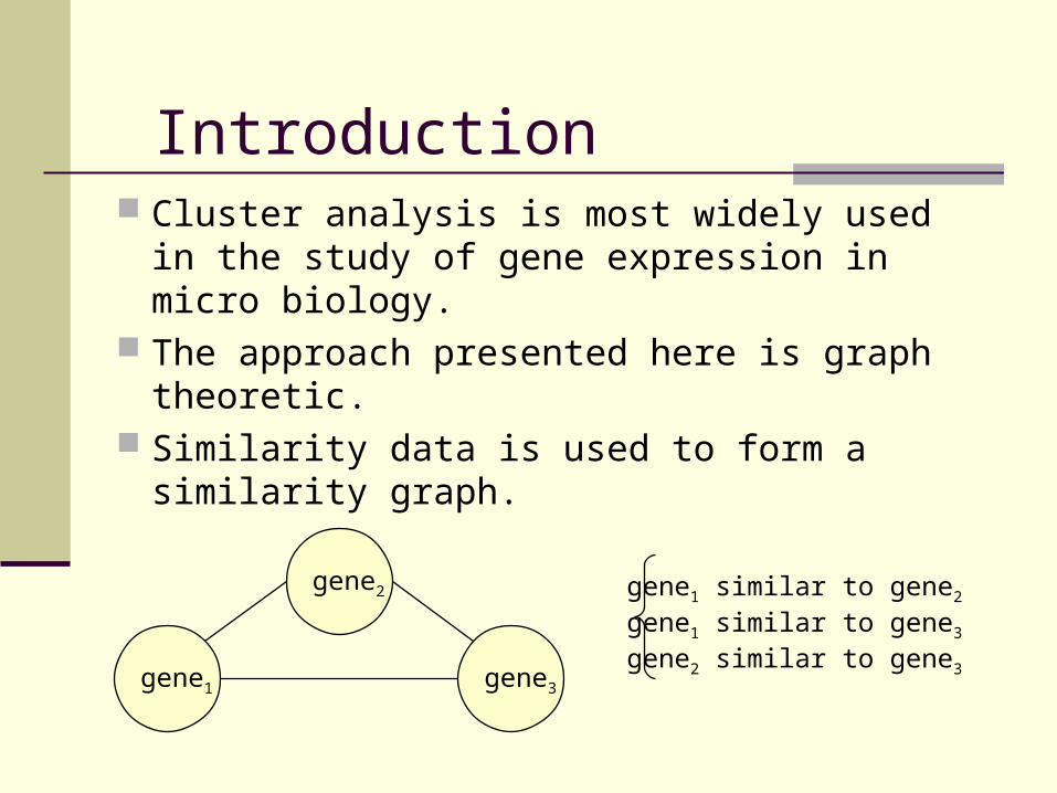
Introduction Cluster analysis is most widely used in the
study of gene expression in micro biology. The approach presented here is graph
theoretic. Similarity data is used to form a similarity
graph.
gene1
gene2
gene3
gene1 similar to gene2
gene1 similar to gene3
gene2 similar to gene3
Introduction In similarity graph data vertices correspond to
elements and edges connect elements with similarity values above some threshold.
Clusters in a graph are highly connected subgraphs.
Main challenges in finding the clusters are: Large sets of data Inaccurate and noisy measurements
Important Definitions in GraphsEdge Connectivity:
It is the minimum number of edges whose removal results in a disconnected graph. It is denoted by k(G).
For a graph G, if k(G) = l then G is called an l-connected graph.

Important Definitions in GraphsExample:
GRAPH 1 GRAPH 2
The edge connectivity for the GRAPH 1 is 2.
The edge connectivity for the GRAPH 2 is 3.
A B
D C
A B
C D

Important Definitions in GraphsCut:
A cut in a graph is a set of edges whose removal disconnects the graph.
A minimum cut is a cut with a minimum number of edges. It is denoted by S.
For a non-trivial graph G iff |S| = k(G).

Important Definitions in GraphsExample:
GRAPH 1 GRAPH 2
The min-cut for GRAPH 1 is across the vertex B or D.
The min-cut for GRAPH 2 is across the vertex A,B,C or D.
A B
D C
A B
C D

Important Definitions in GraphsDistance d(u,v):
The distance d(u,v) between vertices u and v in G is the minimum length of a path joining u and v.
The length of a path is the number of edges in it.

Important Definitions in GraphsDiameter of a connected graph:
It is the longest distance between any two vertices in G. It is denoted by diam(G).
Degree of vertex:
Its is the number of edges incident with the vertex v. It is denoted by deg(v).
The minimum degree of a vertex in G is denoted by delta(G).

Important Definitions in GraphsExample:
d(A,D) = 1 d(B,D) = 2 d(A,E) = 2
Diameter of the above graph = 2
deg(A) = 3 deg(B) = 2 deg(E) = 1
Minimum degree of a vertex in G = 1
A B
D C E

Important Definitions in GraphsHighly connected graph:
For a graph with vertices n > 1 to be highly connected if its edge-connectivity k(G) > n/2.
A highly connected subgraph (HCS) is an induced subgraph H in G such that H is highly connected.
HCS algorithm identifies highly connected subgraphs as clusters.
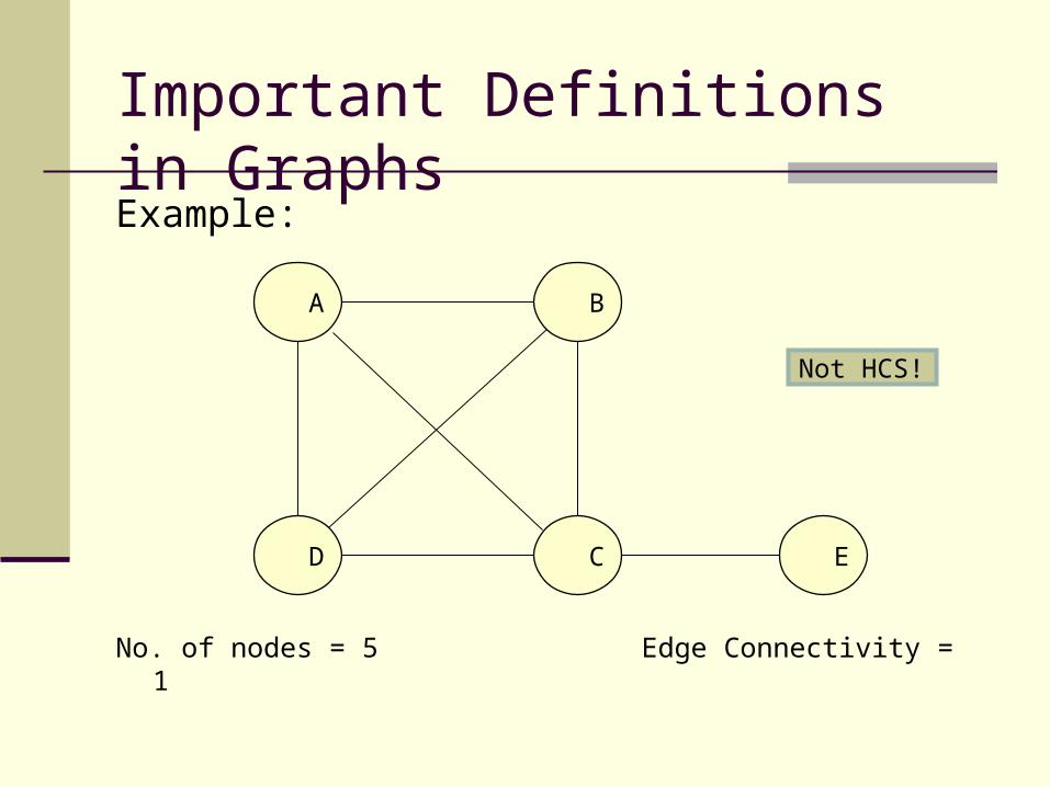
Important Definitions in GraphsExample:
No. of nodes = 5 Edge Connectivity = 1
A B
D C E
Not HCS!

Important Definitions in GraphsExample continued:
No. of nodes = 4 Edge Connectivity = 3
A B
D C
HCS!

HCS AlgorithmHCS(G(V,E))
begin
(H, H’,C) MINCUT(G)
if G is highly connected
then return (G)
else
HCS(H)
HCS(H’)
end if
end

HCS Algorithm The procedure MINCUT(G) returns H, H’ and
C where C is the minimum cut which separates G into the subgraphs H and H’.
Procedure HCS returns a graph in case it identifies it as a cluster.
Single vertices are not considered clusters and are grouped into singletons set S.

HCS AlgorithmExample

HCS AlgorithmExample Continued

HCS AlgorithmExample Continued
Cluster 2
Cluster 1
Cluster 3

HCS Algorithm The running time of the algorithm is bounded by
2N*f(n,m).
N - number of clusters found
f(n,m) – time complexity of computing a minimum cut in a graph with n vertices and m edges
Current fastest deterministic algorithms for finding a minimum cut in an unweighted graph require O(nm) steps.

Properties of HCS Clustering Diameter of every highly connected graph is
at most two.
That is any two vertices are either adjacent or share one or more common neighbors.
This is a strong indication of homogeneity.
Properties of HCS Clustering Each cluster is at least half as dense as a
clique which is another strong indication of homogeneity.
Any non-trivial set split by the algorithm has diameter at least three.
This is a strong indication of the separation property of the solution provided by the HCS algorithm.

Modified HCS AlgorithmExample
Modified HCS AlgorithmExample – Another possible cut

Modified HCS AlgorithmExample – Another possible cut

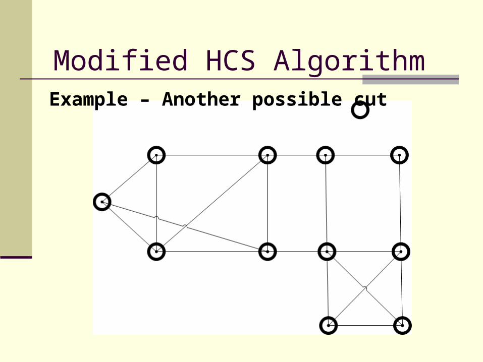
Modified HCS AlgorithmExample – Another possible cut
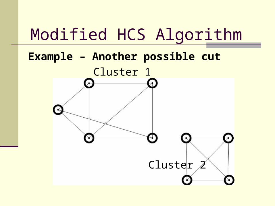
Modified HCS AlgorithmExample – Another possible cut
Cluster 1
Cluster 2
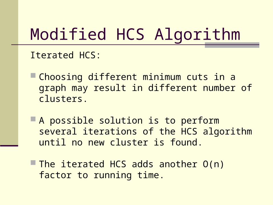
Modified HCS AlgorithmIterated HCS:
Choosing different minimum cuts in a graph may result in different number of clusters.
A possible solution is to perform several iterations of the HCS algorithm until no new cluster is found.
The iterated HCS adds another O(n) factor to running time.

Modified HCS AlgorithmSingletons adoption:
Elements left as singletons can be adopted by clusters based on similarity to the cluster.
For each singleton element, we compute the number of neighbors it has in each cluster and in the singletons set S.
If the maximum number of neighbors is sufficiently large than by the singletons set S, then the element is adopted by one of the clusters.
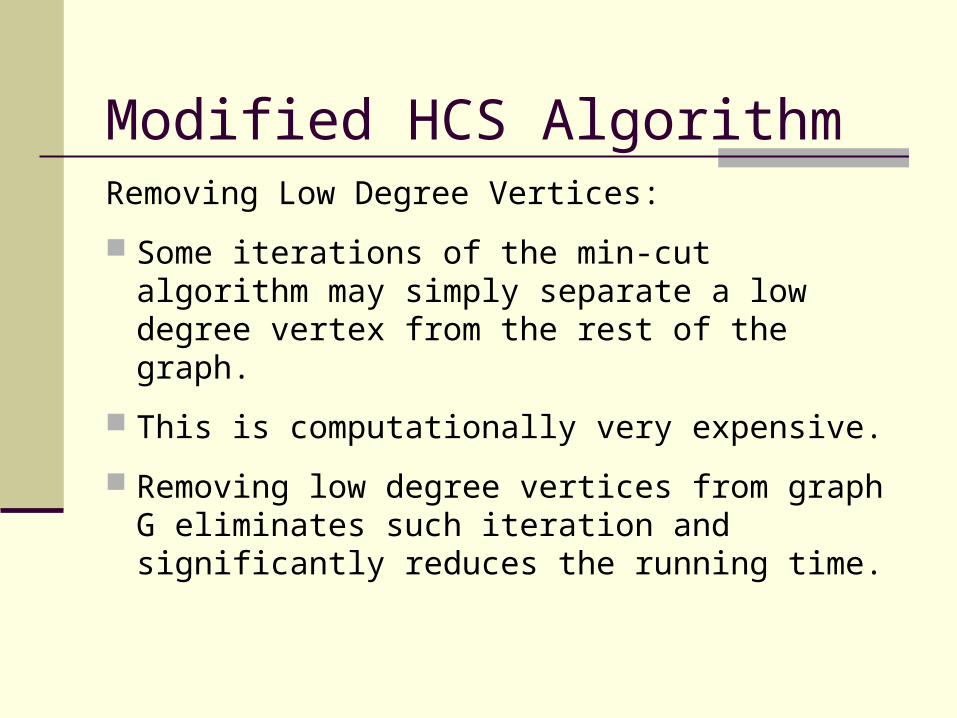
Modified HCS AlgorithmRemoving Low Degree Vertices:
Some iterations of the min-cut algorithm may simply separate a low degree vertex from the rest of the graph.
This is computationally very expensive.
Removing low degree vertices from graph G eliminates such iteration and significantly reduces the running time.
Modified HCS Algorithm
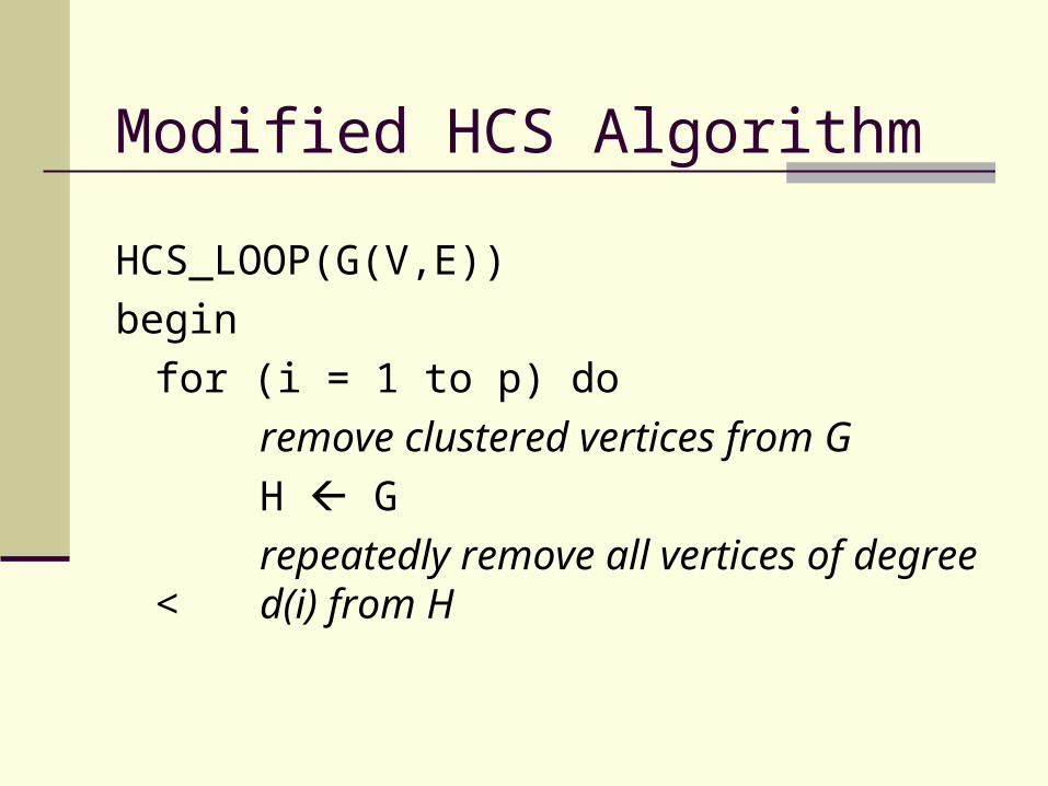
HCS_LOOP(G(V,E))
begin
for (i = 1 to p) do
remove clustered vertices from G
H G
repeatedly remove all vertices of degree < d(i) from H
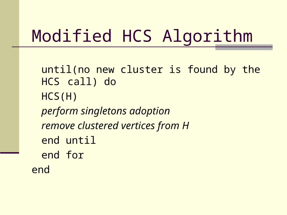
Modified HCS Algorithm
until(no new cluster is found by the HCS call) do
HCS(H)
perform singletons adoption
remove clustered vertices from H
end until
end for
end

Key features of HCS Algorithm HCS algorithm was implemented and tested
on both simulated and real data and it has given good results.
The algorithm was applied to gene expression data.
On ten different datasets, varying in sizes from 60 to 980 elements with 3-13 clusters and high noise rate, HCS achieved average Minkowski score below 0.2.

Key features of HCS Algorithm In comparison greedy algorithm had an
average Minkowski score of 0.4.
Minkowski score: A clustering solution for a set of n elements can
be represented by n x n matrix M. M(i,j) = 1 if i and j are in the same cluster
according to the solution and M(i,j) = 0 otherwise.
If T denotes the matrix of true solution, then Minkowski score of M = ||T-M|| / ||T||
Key features of HCS Algorithm
HCS manifested robustness with respect to higher noise levels.
Next, the algorithm were applied in a blind test to real gene expression data.
It consisted of 2329 elements partitioned into 18 clusters. HCS identified 16 clusters with a score of 0.71 whereas Greedy got a score of 0.77.

Key features of HCS AlgorithmComparison of HCS algorithm with Optimal
Graph theoretic approach to data clustering

Key features of HCS Algorithm For the graph seen previously, with number
of clusters 3 as input, HCS algorithm and Optimal graph theoretic approach to data clustering are compared.
HCS algorithm finds all the three clusters G1, G2 and G3.
Optimal graph theoretic approach to data clustering finds isolated vertex v in {a,b,c,d}. The clusters found by optional approach are two. One is G1\{v} and (G2UG3)\{v}.

Summary
Clusters are defined as subgraphs with connectivity above half the number of vertices
Elements in the clusters generated by HCS algorithm are homogeneous and elements in different clusters have low similarity values
Possible future improvement includes finding maximal highly connected subgraphs and finding a weighted minimum cut in an edge-weighted graph.

Thank You!!


![[2] Corrosion Protection by Design 2014 Balakrishna Palanki](https://static.documents.pub/doc/80x56/577cc5191a28aba7119b4d9b/2-corrosion-protection-by-design-2014-balakrishna-palanki.jpg)


