22
A coarse-to-fine approach for fast deformable object detection Marco Pedersoli Andrea Vedaldi Jordi Gonzàlez
| Date post: | 26-Dec-2015 |
| Category: |
Documents |
| Upload: | gladys-stevenson |
| View: | 215 times |
| Download: | 0 times |

A coarse-to-fine approach for fast deformable object
detection
Marco Pedersoli Andrea Vedaldi Jordi Gonzàlez

[Fischler Elschlager 1973]
Object detection 22
• Addressing the computational bottleneck
- branch-and-bound [Blaschko Lampert 08, Lehmann et al. 09]
- cascades[Viola Jones 01, Vedaldi et al. 09, Felzenszwalb et al 10, Weiss Taskar 10]
- jumping windows [Chum 07]
- sampling windows [Gualdi et al. 10]
- coarse-to-fine [Fleuret German 01, Zhang et al 07, Pedersoli et al. 10]
[Felzenszwalb et al 08]
[Vedaldi Zisserman 2009]
[Zhu et al 10]
[VOC 2010]
Analysis of the cost of pictorial structures
3

• cost of inference
- one part: L
- two parts: L2
- …
- P parts: LP
• with a tree
- using dynamic programming
- PL2
- Polynomial, but still too slow in practice
• with a tree and quadratic springs
- using the distance transform [Felzenszwalb and Huttenlocher 05]
- PL
- In principle, millions of times faster than dynamic programming!
The cost of pictorial structures 44
L = number of part locations ~ number of pixels ~ millions

•Deformable part model [Felzenszwalb et al. 08]
- locations are discrete
- deformations are bounded
55
δ
image
number of possible part locations:
L L / δ2
L2 LC, C << L
cost of placing two parts:
C = max. deformation size
total geometric cost: C PL / δ2
A notable case: deformable part models 5

A notable case: deformable part models
• With deformable part models
- finding the optimal parts configuration is cheap
- distance transform speed-up is limited
• Standard analysis does not account for filtering:
• Typical example
- filter size: F = 6 × 6 × 32
- deformation size: C = 6 × 6
• Filtering dominates the finding the optimal part configuration!
6
C PL / δ2
imageF = size of filter
filtering cost:
F PL / δ2
geometric cost:
total cost: (F + C) PL / δ2
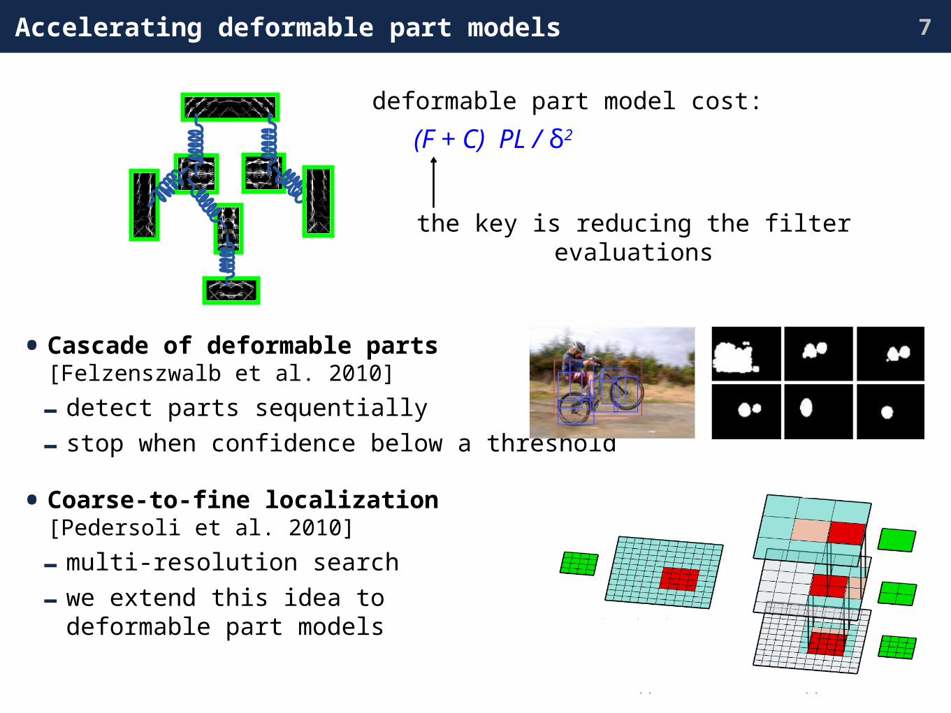
Accelerating deformable part models
• Cascade of deformable parts[Felzenszwalb et al. 2010]
- detect parts sequentially
- stop when confidence below a threshold
• Coarse-to-fine localization[Pedersoli et al. 2010]
- multi-resolution search
- we extend this idea todeformable part models
7
the key is reducing the filter evaluations
deformable part model cost:
(F + C) PL / δ2

Our contribution:Coarse-to-fine for deformable
models
8
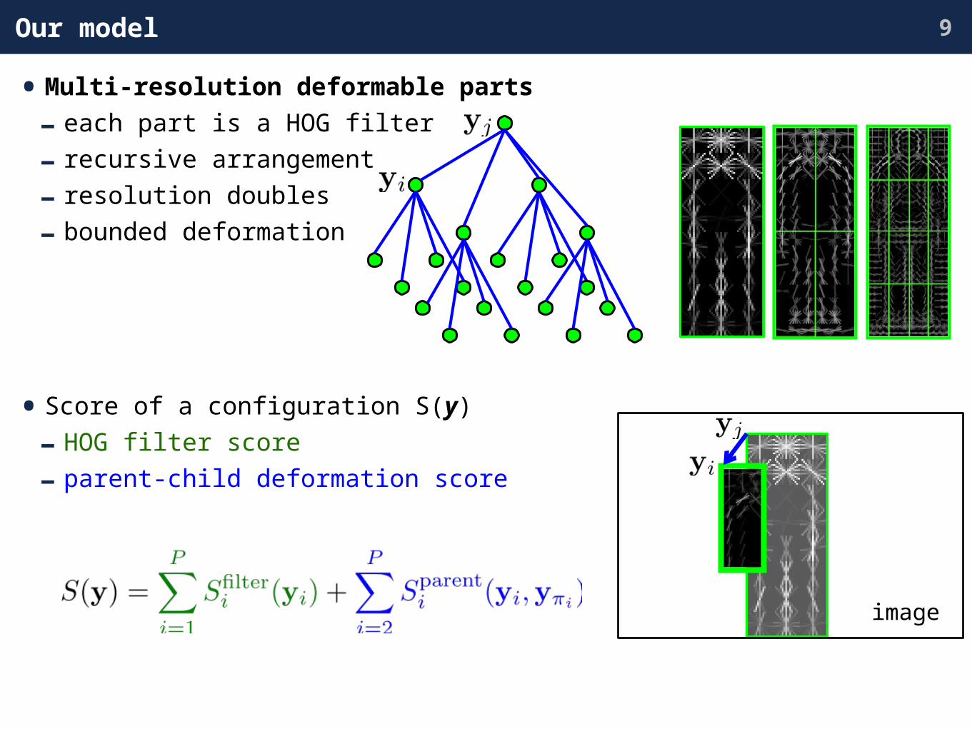
Our model
• Multi-resolution deformable parts
- each part is a HOG filter
- recursive arrangement
- resolution doubles
- bounded deformation
• Score of a configuration S(y)
- HOG filter score
- parent-child deformation score
9
image

Coarse-to-Fine search 10
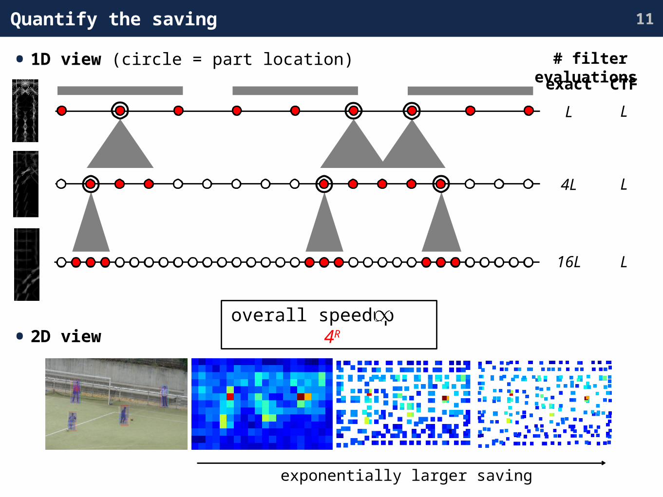
Quantify the saving
• 1D view (circle = part location)
• 2D view
L
4L
16L
exact
L
L
L
CTF
# filter evaluations
overall speedup 4R
exponentially larger saving
11
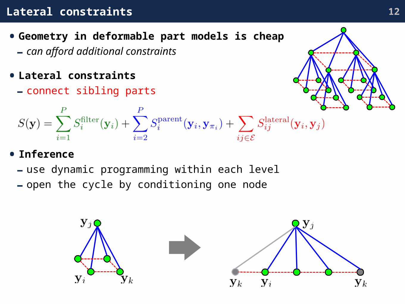
Lateral constraints
• Geometry in deformable part models is cheap
- can afford additional constraints
• Lateral constraints
- connect sibling parts
• Inference
- use dynamic programming within each level
- open the cycle by conditioning one node
12
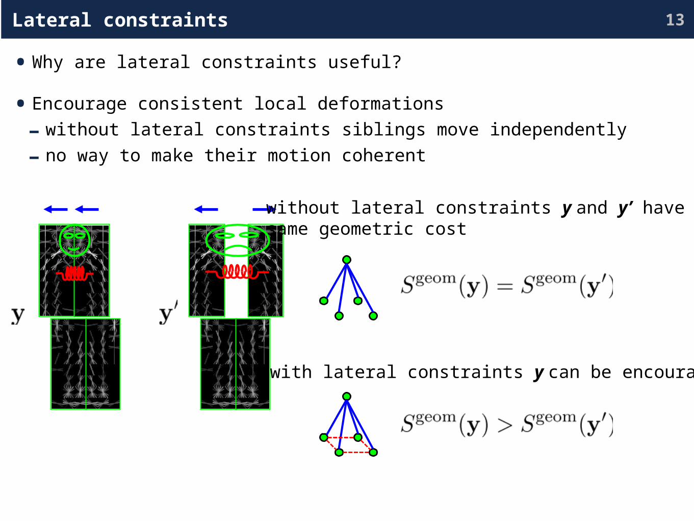
• Why are lateral constraints useful?
• Encourage consistent local deformations
- without lateral constraints siblings move independently
- no way to make their motion coherent
Lateral constraints
without lateral constraints y and y’ have thesame geometric cost
with lateral constraints y can be encouraged
13
Experiments
14

Effect of deformation size
• INRIA pedestrian dataset
- C = deformation size (HOG cells)
- AP = average precision (%)
- Coarse-to-fine (CTF) inference
• Remarks
- large C slows down inference but does not improve precision
- small C implies already substantial part deformation due tomultiple resolutions
C 3×3 5×5 7×7
AP 83.5 83.2 83.6
time 0.33s 2.0s 9.3s
15

Effect of the lateral constraints
• Exact vs Coarse-to-fine (CTF) inference
• CTF ~ exact inference scores
- CTF ≤ exact
- bound is tighter withlateral constraints
• Effect is significant on training as well
- additional coherence avoids spurious solutions
- Examplelearning the head model
• Big improvement with coarse-to-fine search
- Example: learning the head model
• Effect on the inference scores
CTF learning and tree CTF learning and tree + lat.
inference exact inference CTF inference
tree 83.0 AP 80.7 AP
tree + lateral conn. 83.4 AP 83.5 AP
tree tree + lat.
CTF scoreex
act
scor
e
16
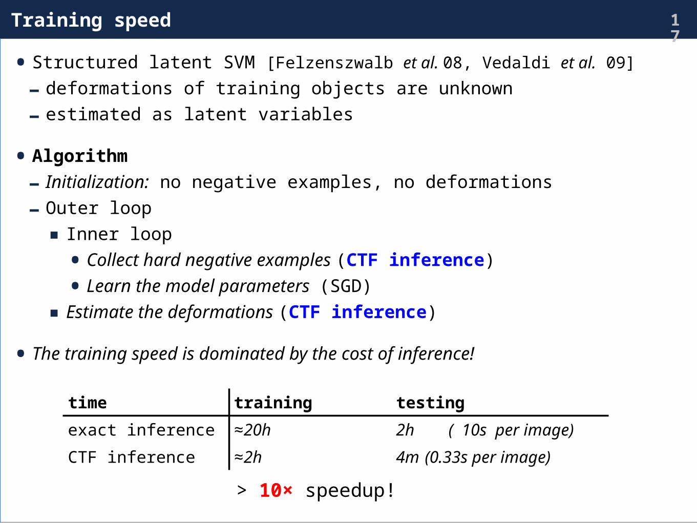
Training speed
• Structured latent SVM [Felzenszwalb et al. 08, Vedaldi et al. 09]
- deformations of training objects are unknown
- estimated as latent variables
• Algorithm
- Initialization: no negative examples, no deformations
- Outer loop
▪Inner loop
• Collect hard negative examples (CTF inference)
• Learn the model parameters (SGD)
▪Estimate the deformations (CTF inference)
• The training speed is dominated by the cost of inference!
17
time training testing
exact inference ≈20h 2h ( 10s per image)
CTF inference ≈2h 4m (0.33s per image)
> 10× speedup!
PASCAL VOC 2007
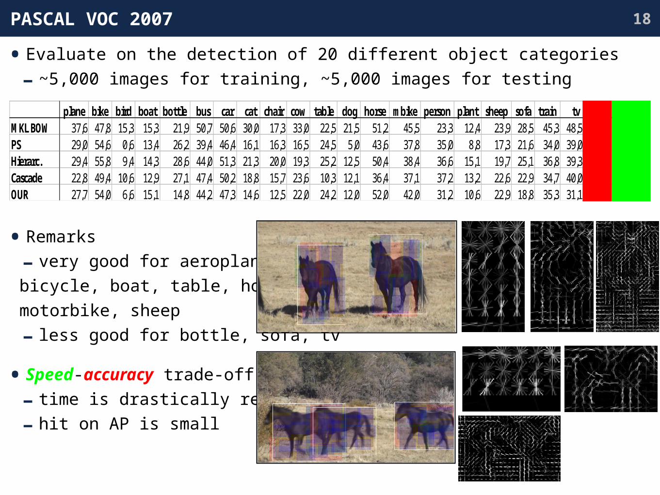
• Evaluate on the detection of 20 different object categories
- ~5,000 images for training, ~5,000 images for testing
• Remarks
- very good for aeroplane,
bicycle, boat, table, horse,
motorbike, sheep
- less good for bottle, sofa, tv
• Speed-accuracy trade-off
- time is drastically reduced
- hit on AP is small
plane bike bird boat bottle bus car cat chair cow table dog horse mbike person plant sheep sofa train tv mean Time (s) MKL BOW 37,6 47,8 15,3 15,3 21,9 50,7 50,6 30,0 17,3 33,0 22,5 21,5 51,2 45,5 23,3 12,4 23,9 28,5 45,3 48,5 32,1 ~ 70 PS 29,0 54,6 0,6 13,4 26,2 39,4 46,4 16,1 16,3 16,5 24,5 5,0 43,6 37,8 35,0 8,8 17,3 21,6 34,0 39,0 26,8 ~ 10 Hierarc. 29,4 55,8 9,4 14,3 28,6 44,0 51,3 21,3 20,0 19,3 25,2 12,5 50,4 38,4 36,6 15,1 19,7 25,1 36,8 39,3 29,6 ~ 8 Cascade 22,8 49,4 10,6 12,9 27,1 47,4 50,2 18,8 15,7 23,6 10,3 12,1 36,4 37,1 37,2 13,2 22,6 22,9 34,7 40,0 27,3 < 1 OUR 27,7 54,0 6,6 15,1 14,8 44,2 47,3 14,6 12,5 22,0 24,2 12,0 52,0 42,0 31,2 10,6 22,9 18,8 35,3 31,1 26,9 < 1
18
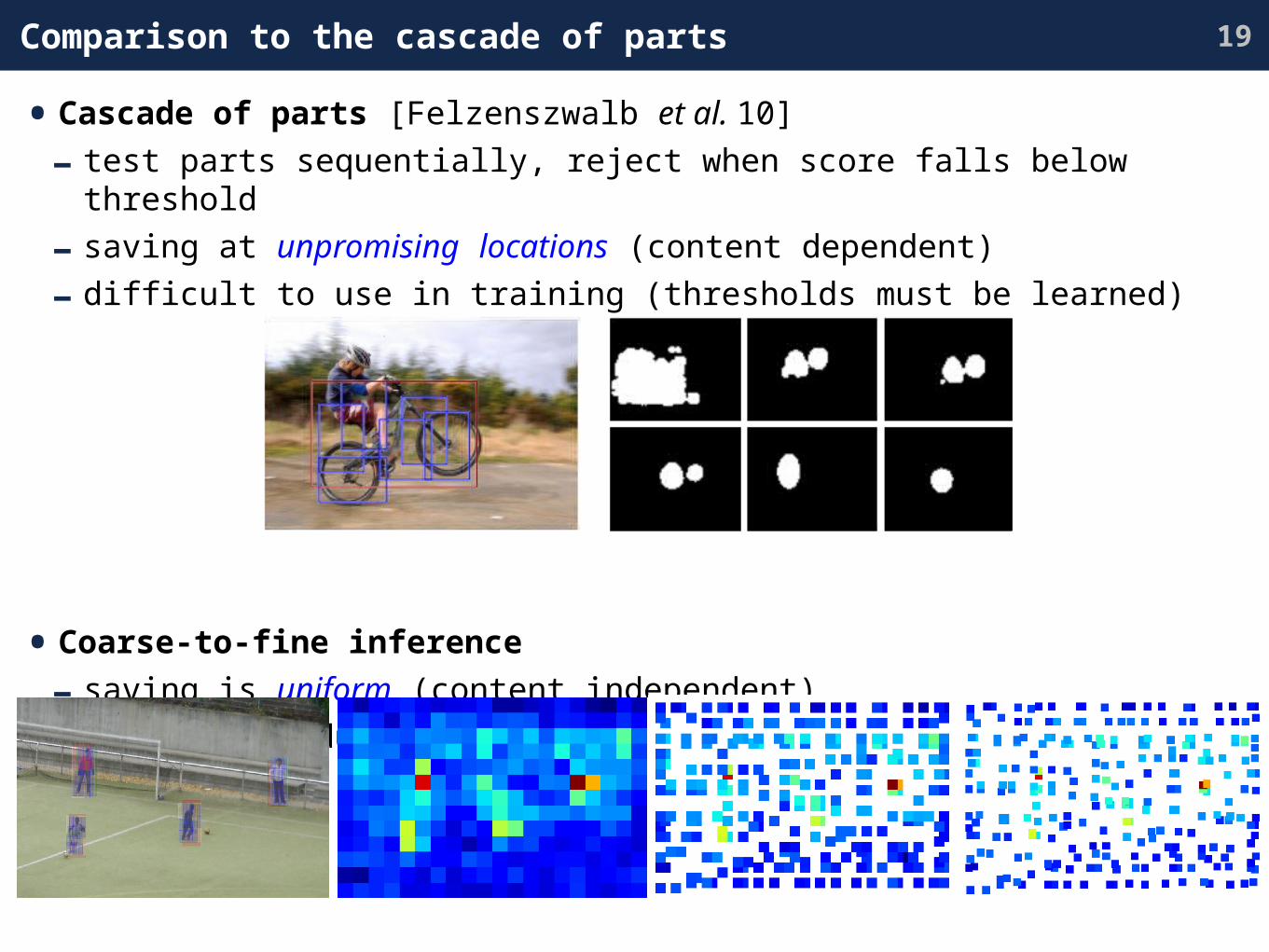
Comparison to the cascade of parts
• Cascade of parts [Felzenszwalb et al. 10]
- test parts sequentially, reject when score falls below threshold
- saving at unpromising locations (content dependent)
- difficult to use in training (thresholds must be learned)
• Coarse-to-fine inference
- saving is uniform (content independent)
- can be used during training
19

Coarse-to-fine cascade of parts
• Cascade and CTF use orthogonal principles
- easily combined
- speed-up multiplies!
• Example
- apply a threshold at the root
- plot AP vs speed-up
- In some cases 100 x speed-upcan be achieved
20
CTF
cascadescore > τ1?
reject
cascadescore > τ2?
reject
CTF CTF
Summary
• Analysis of deformable part models
- filtering dominates the geometric configuration cost
- speed-up requires reducing filtering
• Coarse-to-fine search for deformable models
- lower resolutions can drive the search at higher resolutions
- lateral constraints add coherence to the search
- exponential saving independent of the image content
- can be used for training too
• Practical results
- 10x speed-up on VOC and INRIA with minimum AP loss
- can be combined with cascade of parts for multiplied speedup
• Future
- More complex models with rotation, foreshortening, …
21

Thank you!


![Convolutional Feature Maps - mp7.watson.ibm.commp7.watson.ibm.com/ICCV2015/slides/iccv2015_tutorial_convolutional... · see [Mahendran & Vedaldi, CVPR 2015] Aravindh Mahendran & Andrea](https://static.documents.pub/doc/80x56/5c76d1ff09d3f29a548b72f1/convolutional-feature-maps-mp7-see-mahendran-vedaldi-cvpr-2015-aravindh.jpg)


![Objects in Context - Carnegie Mellon School of … · Analysis: Objects in Context [Rabinovich, Vedaldi, Galleguillos, Wiewiora, Belongie] & Object Categorization using Co-Occurrence,](https://static.documents.pub/doc/80x56/5baa17da09d3f221798bba1d/objects-in-context-carnegie-mellon-school-of-analysis-objects-in-context.jpg)


![arXiv:1805.08136v3 [cs.CV] 24 Jul 2019 · Philip H.S. Torr Andrea Vedaldi FiveAI & University of Oxford University of Oxford philip.torr@eng.ox.ac.uk vedaldi@robots.ox.ac.uk ABSTRACT](https://static.documents.pub/doc/80x56/5ec4943a77a3e52440353613/arxiv180508136v3-cscv-24-jul-2019-philip-hs-torr-andrea-vedaldi-fiveai-.jpg)
