NASA Contractor Report 4078 A Combined Stochastic Feedforward and Feedback Control Design Methodology With Application to Autoland Design Nesim Halyo https://ntrs.nasa.gov/search.jsp?R=19870016373 2018-05-29T16:06:59+00:00Z
Transcript
NASA Contractor Report 4078
A Combined Stochastic Feedforward and Feedback Control Design Methodology With Application to Autoland Design
P W e LATERAL CONTROL STRUCTURE .............................. 83
LATERAL FEEDFORWARD DESIGN MODEL ....................... 84
LATERAL FEEDFORWARD AND FEEDBACK CONTROL GAINS ......... 85 LATERAL EQUIVALENT 8-DOMAIN EIGENVALUES ................ 86 LATERAL SINGULAR VALUES ................................ 87
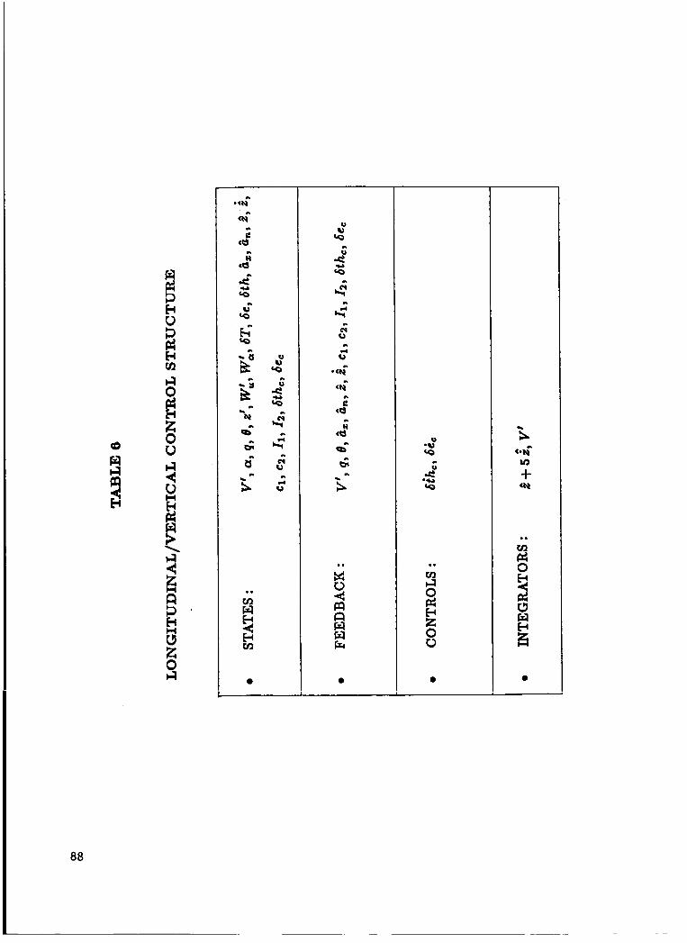
LONGITUDINAL/VERTICAL CONTROL STRUCTURE ................ 88 LONGITUDINAL/VERTICAL FEEDFORWARD DESIGN MODEL ......... 89 LONGITUDINAL/VERTICAL FEEDFORWARD AND FEEDBACK CONTROL GAINS ................................................... 90
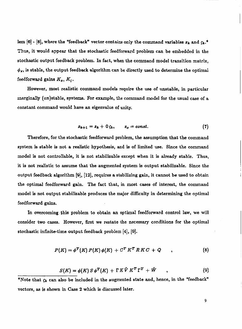
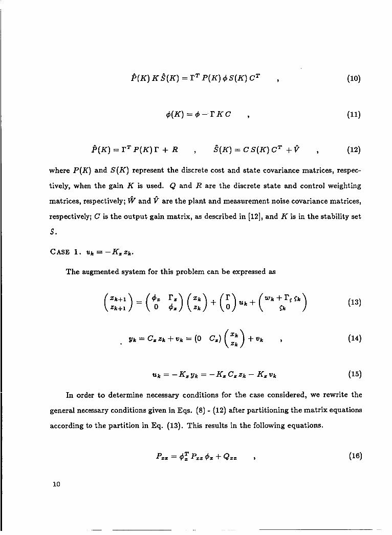
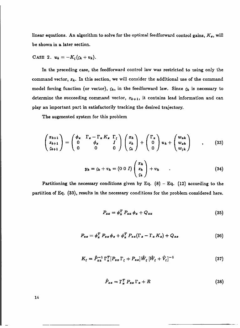
command values, etc. It is possible to use the vector gjk by substituting Eq. (90).
On the other hand, it is often convenient to think in terms of error feedback. So that
a new feedback vector consisting of the error terms defined in Eq. (90) may also be used
in the form of g k - C, H Z k ; i.e.,
g k - C z H Z k = C z x k + l)k + d, (93)
Since the command state, Z k , is known at the kth sampling instant, implementation of the
error feedback vector in real time is clearly possible.
To maintain further generality, we will consider the plant and feedback models in the
form given below
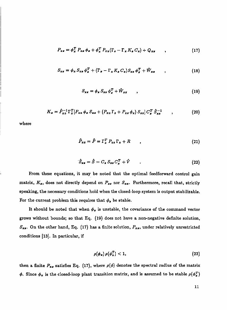
where the standard error feedback case shown above would correspond to C, being null.
t From the limited experience and experimentation performed in this study, it appears
I that better performance is achieved when the error formulation is used in as many vari- I , ables as applicable. Due to the limited time available, the reasons for the differences in
performance or methods for best selection of H were not investigated in this study.
Dynamic Compensation and Integral Feedback.
In many cases, it is of interest to include dynamic compensation in the control law to
achieve particular objectives. The objective may be to estimate a variable for purposes of
feedback, or to provide more robustness or insensitivity.
Similarly, it is usually of interest to have integral feedback of the tracking error, or of
equivalent variables, in order to obtain a type 1 system. To accommodate these often used
control structures, augment the plant state model given in Eq. (94) by the compensator
and integral error models
29
H , = H,C, (98)
Note that the “integrator” is a digitally implementable accumulator. Also note that
the tracking variables, H , y k , have been assumed to be a linear combination of known or
measured, y k , rather than possible unavailable state variables in Z k .
The dynamic compensator is assumed to be of order n, which can be selected arbi-
trarily, according to the desired objectives. The compensator state transition matrix, d C , is also arbitrary, and should be selected in accordance to the cost function which will produce
the closed-loop compensator. The white noise sequences tuck and w r k are included largely
for generality. They could be interpreted as round-off error, variations in H,, jitter, etc.;
however, most importantly, they can be used as design parameters which modulate the
optimal feedback gains.
The basic form of the combined feedforward/feedbak control law is assumed to be
Note that, for the augmented problem, the feedback vector, y k , is also augmented by
the compensator state, C k , and the error integral variables, r k . The feedforward control
law has been constrained to use only the command state and forcing vectors, zk and <k ,
respectively. Finally, fiz and tic are unknown constant (with respect to k) variables arising
30
from the fact that the variables used are not the perturbed values, but correspond to the
total values including the trim values of the variables. As an incremental implementation
will be used, it is not necessary to actually compute the constant vectors.
It should also be noted that the control vector, may be selected to be the rate of the
actual control position variables by augmenting the plant model accordingly. This would
result in a control rate command structure.
Feedback Design Model.
Suppose that the feedforward control sequences { U l k , k 2 0) and { u , f k , k 2 0) pro-
duce a satisfactory trajectory. Then, when no plant noise or measurement noise is present,
then trajectory will be given by
Since the actual plant, compensator and integral states evolve according to Eq. (94),
Eq. (96) and Eq. (97), respectively, the deviations, or error, in these variables can be
defined as
Manipulating, it is seen that the error in the state has the dynamics
The deviations in the actual state relative to the desired trajectory are seen to be due
to plant and measurement noise, and initial condition mismatch. Of course, in practice
these deviations are also due to changing plant parameter values, unmodeled nonlinearities,
unmodeled dynamics, sampling errors, etc.
Since all the terms containing the command model have canceled, the deviation about
the desired trajectory is seen to be independent of the command state. Thus, the possibly
unstable command model has no direct impact on the feedback control law design. Where
highly nonlinear effects which involve the command state exist, the command may not
cancel; however, this is not a usually encountered case.
Therefore, the design of the feedback control law can be done largely independently of
the feedforward control law. The usual major objectives of feedback, such as stability about
the desired trajectory in the presence of disturbances and despite unceriaiiitk &hut , &id
variations in, the plant models, can thus be pursued using the dynamical system describing
the deviations about the desired trajectory in Eq. (107) - Eq. (110 ).
The feedback vector, in this case, is taken to be (6,' C"f fr)T. So that a control law
of the form
32
can be designed using any modem or classical control design technique. In particular,
note that stochastic output feedback [ll], [ 121, multi-configuration control or decentralized
control techniques [13] can be used for this purpose. In the following, it will be assumed
that the feedback control law thus designed stabilizes the closed-loop system.
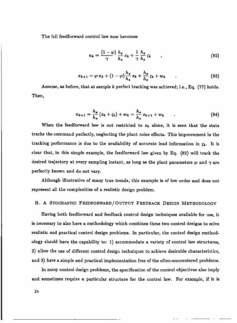
Feedforward Control Model.
Having designed a satisfactory feedback control law, recall that the feedforward control
in Eq. (101) - Eq. (104) is arbitrary, and can now be selected using a stable closed-loop
system.
Consider the following change of variables in the control vectors u:k and UZk.
Substituting these expressions into Eq. (101) - Eq. (104), we obtain the feedforward
control model
where
are constant vectors depending on the trim conditions for the particular operating points
used.
From the discussion above, it is clear that the feedforward control design problem is
one finding control sequences {& , k 2 0) and { P E k , k 2 0) in terms of a given subset of
the augmented state variables z;, c;, I;, and zk, 6, when the command state transition
matrix &, is not necessarily stable, such that { H y y; - Hz Zk , k 2 0) is as "small" as
possible.
A full analysis of the many interesting cases where different subsets of the augmented
feedforward model state are selected is beyond the scope of the current study. Only the
two cases solved in the preceding section will be treated in some detail. However, the full
state feedback case is worthy of note.
Consider the case where the feedforward control law form is unrestricted and { I & ,
k 2 0 ) is a Gaussian white noise process, with all initial conditions also being jointly
Gaussian. With a quadratic cost function, it is well-known [4] that the optimal control
is the solution to the LQG problem. The case where the plant contains unstable and
uncontrollable modes, has been treated by the author as a disturbance accommodation
problem [8], (71. It is clear that the most accurate feedforward control law would be
obtained by this unconstrained solution.
34
While this solution has a variety of desirable characteristics, it also has a disadvantage.
It requires the computation of the augmented desired trajectory z;, c; , I;, Z k , ck as a
part of the feedforward controller. With the increasing speed and memory capabilities of
flight computers, this is not necessarily impractical, but will not be pursued further in this
study.
Now consider the case where the feedforward control is restricted to the form
Using a quadratic cost function of the form of Eq. (5 ) which includes the most common
~ case
1 I
it is possible to obtain the optimal feedforward gains K z z , KZs, Kc,, and Kcs.
It is important to note that the treatment of the feedforward control law in the
preceding section accommodates the cases where any one of the feedforward gains is set
to zero or some other constant.
,
I
To obtain the total control law, recall that from Eq. (105),
The combined feedforward/feedback control law with dynamic compensation and in-
tegral error feedback can be obtained by closing the loop on the compensation in Eq. (96)
with Eq. (125).
Of course, it is also necessary to compute and update the command state and forcing
vectors, Zk and h, respectively, according to the desired trajectory. Note that since the
feedforward law only uses the current values Zk and $k, these commands need not be
available ahead of time and could be real-time pilot inputs or may be computed from
real-time pilot inputs.
C. IMPLEMENTATION
While Eq. (126) - Eq. (128) with the addition of the command state and forcing
vector constitute the combined feedforward/feedback control law, there are a number of
advantages to implementing the control law in incremental form.
First note that the constant terms pi and pz have not been determined. Even though
it is possible to compute these vectors using trim conditions, it is more convenient if the
control law were not to require these vectors. A second advantage to an incremental
implementation is the elimination of the integral terms. When the tracking error is, at
least temporarily, large, the integral state I k can reach very high values. This usually leads
to the control commands reaching limits. Even though the tracking error may have been
reduced to small levels, it can take a considerable amount of time before the integral state
36
~
reaches reasonable levels, and the limiting of the controls is eliminated. The unnecessary I I I I ~ an incremental implementation.
i
effects of this phenomenon, referred to as "integral wind-up" can largely be eliminated by
By simply differencing the control law,
When UZk has been modeled as a control rate command with a zero order hold, the actual
control position commanded is given by 6k.
where the control position command 6 k is part of the state Z k . Other holds will result in
similar expressions.
Thus, the actual implemented digital control law is given by Eq. (129) - Eq. (133). It is seen that the constant terms depending on the trim conditions have canceled out and
do not appear in this implementation.
37
It should be noted that the initial condition for the error integrator states, I,, is not
needed in this implementation. Only the initial control variables uzo, and sometimes So,
and the initial compensator increment Ac, are needed at initialization. The initial condi-
tions for the control variables can be set equal to the actual control values at initialization.
When a dynamic compensator is designed, the best selection of the initial compensator
value is not clear; however, in many cases, the objective of the compensator and the initial
plant operating point provide a good choice. For example, when the plant initially is in
trim (i.e., in a steady state condition), the initial compensator increment, Ac,, would be
selected as zero. According to circumstances, other choices are possible. A more detailed
study of the selection of the initial conditions, particularly when obvious choices are not
available, is necessary.
When the plant, due to mechanical reasons, has limiting effects on the movement of
the actual control variables, it is desirable not to command the controls to exceed these
limits since such commands will not be followed. Therefore, it is often desirable to have
control rate and control position limits set in the control law. In this implementation, such
limits are easy to implement and generally have little negative impact. Rate limits can be
applied to uzk and position limits to 6k.
It is important to distinguish between limiting action due to the feedforward com-
mands as opposed to feedback related commands. It is important to note that, in a
satisfactory design, there should be no plant limiting due to feedforward commands, ex-
cept in some circumstances. The feedforward control design should include an analysis of
maximum control commands implied by the class of commanded trajectories. In general,
the p!zzt !kitkg cszditio~s ehiiiiX 'ut: avoided by appropriate changes in the command
state and forcing vector.
In other words, the feedforward design philosophy proposed taken here is to command
only trajectories which can physically be achieved by the plant, and avoid,using up the
control authority in the feedforward control, thus leaving some control authority to the
38
feedback controller. This has two desirable effects. The first is to allow the feedback
controller to close the loop and provide its main objective; i.e., stability. This is of utmost
importance in plants which are open-loop unstable or have relaxed static stability, as is
the case with many high performance aircraft. If the feedforward commands were to reach
the plant control limits, the feedback law would not be able to close the loop and perform
its critical objectives. The second effect of this philosophy is to maintain the nonlinearities
in the command model generating the desired trajectory. If an unachieveable trajectory is
commanded, the precise outcome is not clear; i.e., the actual and desired trajectories will
diverge; however, the nature of the divergence is no longer controlled, and how to recover
from the divergence is not clear. Whereas by commanding and tracking a trajectory which
may be somewhat different than originally desired, tracking control is maintained, and
can be used to converge with the originally desired trajectory. The ease with which such
nonlinear command models can be implemented digitally, as opposed to analog designs, is
also worthy of note.
Finally, the usual type of “integrator wind-up” is eliminated in this implementation
since the integral itself is not explicitly computed. Of course, when no limiting occurs,
the effect of the integrator is unchanged; the integration is simply performed at a different
location, namely in Eq. (131). However, when (nonlinear) limiting occurs, the effects are
usually much more benign.
Eigenvalues of Implementation.
Since the implementation is obtained by differencing the control law designed, it would
result in the same numerical control commands when all initial conditions are appropriately
matched, no nonlinearities and no random disturbances are present. However, since these
conditions rarely, if at all, hold, the implemented and designed control commands are not
the same.
It is important to note that the implemented control law is closely related to but
different than the designed law. For example, the implemented law depends on both yk
39
and y k - 1 , whereas the designed law only uses y k . It is therefore necessary to investigate
the closed-loop characteristics of the implemented control law.
After some manipulation, the implemented closed-loop system can be written as
z k + 1 dz - I ' zKzycz -rzKzc - r z K z ~ I'zKzyCz rz 0 0 0 0 0
[ si.] (134) where the command model state and forcing vector, Zk and Ck, and the constant vector d k
have been set t o zero as they do not affect or modify the closed-loop eigenvalues.
-KcyCz 4 c - K c c - K ~ I K c y c z
0 0 0 X k - 1
i21:) = [ AtH,C, I z k
u z k - K Z & Z - K z c - K ~ I KzyCz I U z k - 1
It is clear that the stability of the implemented closed-loop system is determined by
the eigenvalues of the matrix, @ I , rather than the eigenvalues of the designed closed-loop
where 6A and 6R represent the actual aileron and rudder surface positions, while 6Ac
and 6Rc represent the aileron and rudder commands generated by the control law, respec-
tively, and t j is the dynamic pressure. The variables rl and r2 are inner loop (yaw damper)
variables which will be discussed in more detail later. The aileron and rudder actuator
models given above are linearized and approximated versions of nonlinear systems contain-
ing servomechanisms, hydraulic and mechanical systems with usual nonlinearities such as
hysteresis and limiting effects. A more detailed discussion of the actuator systems on the
ATOPS research vehicle can be found in [IS]. The spoiler is not used as an independent
control surface, but rather as an aid in producing further rolling moment during turns in
c c c p e r ~ t i c ~ :...it!: $!:e zi!e:~; g i i f~ee . This k ~&ie-;eij M B i idif ies i p i ~ ~ i ~ ~ i i i i & gain
on the flight computers, which is approximated to a simple linear relation in the design
model.
6sp = 1.736A .
48
The ATOPS research aircraft incorporates a yaw damper. In the design of the auto-
matic landing system, the yaw damper is taken to be part of the basic airplane stability
control system and interpreted as an inner loop system which will be part of the overall
controller. The yaw damper model given below is therefore included in the design model
of the open-loop plant.
+2 = -6.993 r2 + 10.7485 r , (169)
where r is the yaw rate, modeled by Eq. (156). The variables r1 and r2 are then used to
generate the overall rudder command as shown in the rudder actuator model in Eq. (165).
Another system that is included in the design model as part of the open-loop plant is
a third order complementary filter. This filter uses a body-mounted accelerometer triad
along with position information from the Microwave Landing System (MLS) to obtain
estimates of the aircraft velocity in the Earth coordinate system. The complementary
filter is approximated as follows. I
I
(173)
49
where uy is the body-mounted accelerometer reading for the x-axis, while a: is its normal-
ized form and 510 the filtered acceleration, zll and 5 1 2 are the filtered aircraft distance
from the runway centerline and z 1 2 its rate of change.
As mentioned earlier, the control variables are the aileron and rudder commands 6Ac
and 6Rc, respectively. A rate command structure is used in the design of the control law,
even though the actual implementation will command the surface positions.
6Rck+l = 6Rck + Atu2k 9 (175)
where At is the sampling interval of the control law.
The design model accommodates a second order dynamic compensator, even though
the actual design does not use the dynamic compensator. However, the model is given
here for completeness.
c2k+l = e-6AtC2k + At U&k 9 (177)
Finally, the control law structure is modeled with two integrators, shown below as
digital accumulators.
I Z k + l = I2k + At((Pk - (Pck) 9 (179)
where &k,
commanded values will be defined in the command model.
and P c k are the commanded values for yk, y k and P k , respectively. These
50
The open-loop plant model used for the design of the lateral control law is obtained
by the augmented system consisting of the state equations (154) - (159), (164) - (166),
(168) - (172) and (174) - (179). It is important to note that Eqs. (174) - (179) which
contain the digital controller structure are defined in discrete form in exactly the way
that they will be implemented. Whereas the remaining equations of the design model are
given in differential equation form as they model continuous processes. The latter set of
I
I equations must first be discretized using the usual sampled-data formulation [19] based on
the assumption that 6Ac and 6Rc remain constant over the sampling interval. Then this
set of discrete equations are augmented by the already discrete set (174) - (179) to obtain
the complete discrete design model for the open-loop plant of 20fh order.
I Lateral Command Design Model. I
I While the design model of the open-loop plant developed in the preceding is suffi-
cient to design the feedback control law, the feedforward control law design requires the I I I command design model. The command design model is used to obtain the structure and I
gains of the control law; however, the implementation of the actual commands may use a
somewhat different set of equations as will be discussed in more detail in the following.
The lateral co&and model is selected to be the 4th order system given by
The command model state vector, z k , is
The resulting command model is
1 A t O 0 0 1 0 0
..=(O 0 1 At) '
0 0 0 1
As can be seen from the open-loop plant design model integral feedback equations
(178) and (179), the tracking variables are the lateral position y and the roll angle p. In
the case of the y-position, a linear combination of the position and velocity is used as
the error integral feedback. Furthermore, since the actual position and velocity are not
known, their estimates as obtained from the third order complementary filter are used in
the feedback loop; thus, the position tracking error is defined to be
(6; - Y t k ) + 5(& - Y r k ) 3 (189)
while the bank angle error is simply the difference p k - p c k .
An error formulation of the type described in the previous section is used for the
design of the controller. The variables in which error terms are formed are the roll angle
p, the roll rate p, the lateral position y , the yaw angle $, and the lateral position and
52
velocity estimates from the complementary filter. The yaw angle command used is the
desired track angle. With this definition of H in the error formulation Eq. (180) becomes
The error formulation of the open-loop plant model thus obtained is then used in
designing the feedforward and feedback control laws. Table 1 shows the feedback vector
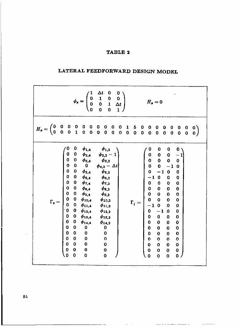
and summarizes the structure of the controller. Table 2 shows the feedforward matrices
r X and rS which apply to the error formulation of the open-loop design model.
While the command design model is given by Eqs. (181) - (188), the on-line generation
of the actually commanded path is obtained using a more complex procedure. The lateral
trajectory followed by the aircraft may be divided into two portions: the localizer capture
path and the localizer. The localizer beam is assumed to be on the runway centerline.
Figure 2 shows the basic geometry of lateral maneuvers. When the controller is
engaged, the aircraft heading tl0, is extended until it intersects the runway centerline
(hence the localizer) at X I . It is assumed that the initial aircraft position and heading
are such that the aircraft would intersect the runway centerline if the heading remained
constant. A new independent variable, R, is defined as follows.
(192) $0 $0 R = (z - X I ) cos - + y s i n - , 2 2
As can be seen from Figure 2, R is measured along the bisector of the heading tlr0 at the
localizer intercept point, X I ; it is the position component of the aircraft along this bisector;
i.e., R is the distance between the localizer intercept point, X I , and the intersection of the
perpendicular to the bisector. The localizer capture command path is defined with R as
the independent variable.
53
The command path prior to the initiation of the localizer capture mode simply follows
a straight line along the initial heading of 9,. The localizer capture path is commanded
when the capture criterion is satisfied, at R = R,. The localizer capture path is a smooth
curve with continuous first and second derivatives at both capture initiation and termi-
nation. At R = R, + P , the commanded localizer capture path smoothly transitions into
the straight-in localizer portion. The decrab mode is initiated when the decrab altitude is
reached and continues until touchdown. I Thus, the actual lateral command path is generated using the equations
(2 - x r ) tan$, R < RO or JLOC = F Y & < R < & + P
R > R o + P
R = 5 cos- 90 -+ 6 sin- 90 , v G = J m , 2 2
(193)
where v~ is the estimated ground speed.
The smoothness of the localizer capture path is due to the selection of the functions
fo(R) and j l ( R ) . Over the interval [-$ $1, these functions are defined by
f i ( R ) = f i (Ro) + A 27r P (197)
54
where fo(Ro), fl(&), Ro, P and A are arbitrary parameters. These parameters are
selected so as to satisfy the boundary conditions of continuity of the first and second
derivatives of fo (R) , namely fl(R) and f z ( R ) , at both ends of the interval [-v, P P ?] with
the adjoining paths, resulting in
1 $0
A 2 , R o = - s i n - 2 $0 p=-- A sin -
2
$0 , f l (R0) = 2 s i n - 2 2 $0 fo(R0) = - s i n - A 2 2
where VO is the commanded airspeed and lfilmoz is the maximum inertial lateral accelera-
tion which will be required to track y, perfectly. Since ljilma2 is a measure of the sharpness
of the capture and of the maximum bank angle required, it is left as a parameter to be
selected by the flight experimenter. When ljilmoz is increased the localizer capture ma-
neuver will be engaged closer to the localizer and will be performed more quickly using a
higher bank angle.
The localizer capture criterion resulting from this trajectory is to engage the capture
mode when
2 1c15 1 (2vo s i n +) IYlm4z
, is satisfied for the first time.
The commands for the roll angle, cp,, are chosen so as to produce a coordinated turn
when perfect tracking is achieved. The commanded track angle can be found to be
55
Accordingly, the commanded roll is selected to be
When the decrab altitude is reached, the commanded roll angle is selected so as to
roll into the wind and perform a sideslip maneuver
The actual command vector used on-line is thus obtained using the set of equations
described above. On the other hand, the design of the control gains uses the command
design model given by Equations (181) - (184). Using the design models for the open-loop
plant and controller structure and the command trajectory, the feedback and feedforward
design for the lateral control law is obtained using the stochastic feedforward and output
feedback approach described in the previous section. The analysis and simulation results
will be described in the next section.
B. LONGITUDINAL CONTROL LAW DESIGN
The longitudinal control law design is performed following the same approach as the
lateral control law. Although the flight maneuvers performed in the longitudinal vertical
plane are different than the lateral maneuvers, command path models similar to the lateral
capture can be used in the glideslope capture and flare maneuvers. As in the lateral case,
a longitudinal plant design model and a command design model are needed to obtain the
longitudinal control law.
Longitudinal Plant Design Model.
The plant design model is obtained by combining the aircraft's longitudinal aerody-
namics and kinematics model with the control actuator and complementary filter models,
and then augmenting the resulting model with the controller model consisting of dynamic
56
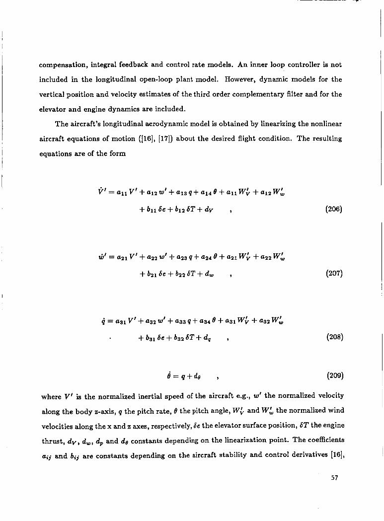
compensation, integral feedback and control rate models. An inner loop controller is not
included in the longitudinal open-loop plant model. However, dynamic models for the
vertical position and velocity estimates of the third order complementary filter and for the
elevator and engine dynamics are included.
The aircraft's longitudinal aerodynamic model is obtained by linearizing the nonlinear
aircraft equations of motion ([16], [17]) about the desired flight condition. The resulting
equations are of the form
where V' is the normalized inertial speed of the aircraft e.g., w f the normalized velocity
along the body z-axis, q the pitch rate, 8 the pitch angle, W& and Wh the normalized wind
velocities along the x and z axes, respectively, 6e the elevator surface position, 6T the engine
thrust, dV, dw, dp and de constants depending on the linearization point. The coefficients
aij and 6 i j are constants depending on the aircraft stability and control derivatives [16],
57
[17], [14]. The normalization factor for the affected variables is the aircraft's nominal
airspeed, V,.
It should be noted that, due to the presence of the linearization constants d v , d,, d,
and de, the state variables VI, W', q and 0 are not the usual perturbations but the total
value of these variables.
~
The design model for the longitudinal wind velocity components Wb and W$ is taken
to consist of first order dynamics in each of the velocity components. Thus,
w; = -0.1 w; + w, 3
where w v and w, are assumed to be independent white noise processes driving the wind
model.
The position of the aircraft c.g. along the Earth-fixed x and z axes can be obtained
from the kinematic equations. The general kinematic equations can be expressed as
i t= -V'sin 7 , (213)
where V& is the normalized ground speed, $T the track angle and 7 the flight path angle.
In the plant design model used here, the position along the Earth-fixed x-axis is taken
as the independent variable, and is not modeled as a state variable. Accordingly, the
expression for i given in Eq. (212) is not a state equation. On the other hand, the vertical
position z is modeled as a state variable. After some manipulation, Eq. (213) can be
approximated in the form
58
9 (214) I Et = COS r0 w - COS r0 8 - sin r0 VI + d,
where r0 is the nominal flight path angle.
The longitudinal controls used are the elevator surface position, 6e, and the engine
thrust, 62'. The control actuator models used for design purposes are given by
10.76 1 + 0.00236 61 = -23.23 6e + 2.0779 9
6 T = -0.5 6T + 0.298 6th , (216)
6t'h = -6th + 6thc 9 (217)
where 6ec and 6thc represent the commanded elevator and throttle positions, respectively,
and 6th the throttle position. The elevator actuator model includes the effect of cable
stretch due to aerodynamic loading on the surface. It is also important to note that the
engine dynamics are actually rather nonlinear, and respond faster when reducing thrust
than when increasing thrust. A linear approximation to the latter condition has been used
in the design model in Eq. (216). A 1 second time constant is used to model the throttle
servo dynamics. Rate limiting and other nonlinear effects are not included in the open-loop
plant design model.
The third order complementary filter is modeled by
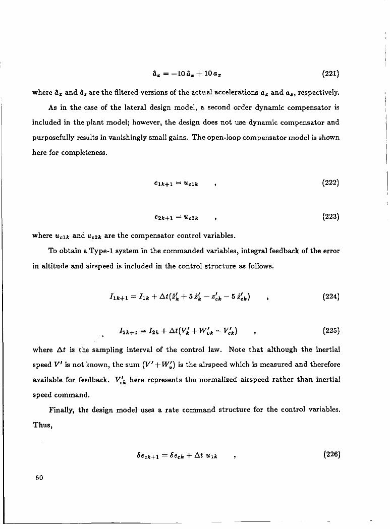
O = 0.82 - 0.8; + E
b, = -lo&, + loa,
a, = -10 a, + 10 a,
where 8, and 8, are the filtered versions of the actual accelerations a, and a,, respectively.
As in the case of the lateral design model, a second order dynamic compensator is
included in the plant model; however, the design does not use dynamic compensator and
purposefully results in vanishingly small gains. The open-loop compensator model is shown
here for completeness.
(221)
C Z k + l = u c 2 k 9
where u c l k and Ucqk are the compensator control variables.
To obtain a Type-1 system in the commanded variables, integral feedback of the error
in altitude and airspeed is included in the control structure as follows.
I 2 k + l = 1 2 k -k At(vL -k W:k - v i k ) 9 (225)
where At is the sampling interval of the control law. Note that although the inertial
speed V' is not known, the sum (V'+W:) is the airspeed which is measured and therefore
available for feedback. v f 'k here represents the normalized airspeed rather than inertial
speed command.
Finally, the design model uses a rate command structure for the control variables.
Thus ,
where U l k and u 2 k are the control variables of the open-loop plant design model thus
obtained.
When the continuous system model described by linear differential equations are dis-
cretized using the standard stochastic sampled-data formulation and the digital controller
model is added, the discrete plant design model of 20fh order is obtained.
To avoid confusing the vertical position variable, z , with the command state vector,
the latter is denoted by 2 in Eq. (228) and in the following.
Longitudinal Command Design Model.
The longitudinal variables used in the design, as indicated by the error integral feed-
back variables in Eqs. (224) and (225), are the airspeed and a linear combination of the
vertical position and its rate of change. Note that this linear combination may be inter-
preted as the predicted value of the vertical position in 5 seconds. Also recall that since
the Earth-fixed z-axis is defined positive downward, the vertical position, z, is the negative
of the c.g. altitude, h.
The longitudinal command model selected for designing the feedforward control gains
is the 2"d order system given by
The command state vector Z k corresponds to (ZLk V&)T, where z r k is the normalized
vertical position command and v& is the normalized airspeed command.
An error formulation is also used in the longitudinal control law. Thus, error terms
are formed in the normalized vertical position, z, the complementary filtered estimate of
the vertical position, 9 , and the airspeed, V. With this definition of the matrix H, the
plant equations become
While the command design model given by Eqs. (229) and (230) are used to design the
feedforward control gains, the actually commanded path is obtained as follows. Initially,
the aircraft is assumed to be in level flight prior to the glideslope capture maneuver. The
initial altitude of the aircraft is maintained until the glideslope capture criterion is satisfied,
at which time the desired glideslope capture path is commanded. When the capture is
completed, the desired glideslope is the vertical path commanded until the flare initiation
criterion is satisfied. At that time, the altitude profile corresponding to the flare path is
commanded until touchdown.
The same functions fo, f l and fi which have been used in the lateral command path
generation are used in generating the glideslope capture and flare path. An important
characteristic of these paths is their smoothness. The independent variable used in the
longitudinal path command is the x-position of the aircraft c.g. in the Earth-fixed coor-
dinate frame. The commanded path is given here as the altitude, h, which corresponds
to the negative of the vertical position, z. Thus, the glideslope capture and flare vertical
profiles are generated using the basic form
62
27r(z + Az) P - A (g) (1 + COS
2 s ( z + Az) P
where 50 corresponds to the initiation of the maneuver, and the constants are selected
according to whether the glideslope capture or flare maneuver is to be performed. The
altitude, sink rate and vertical acceleration are given by
The glideslope capture path starts from level flight and smoothly transitions to the
desired glideslope angle 7 ~ s . When the capture path starts at an altitude hGC and
requires a vertical acceleration no larger than ILImaz, the parameters of the path given by
Eqs. (234) - (235) are
Thus, when the aircraft is at an initial altitude hGC and must track the glideslope 7cs
without exceeding lilmaz of vertical acceleration the vertical profile given by Eq. (234)
6 3
using the parameters in Eqs. (238) - (240) will be denoted by ~ G C ( Z ) = ~ O G C ( Z ) , ~ I G C ( S )
and h z ~ c ( z ) . It should be noted that the smoothness of the glideslope capture can be
easily adjusted by selecting the appropriate value for lilmaz. The criterion for initiating the glideslope capture can be expressed as follows. Com-
mand the path h o ~ c ( z ) when the inequality
A
(241) PGC
i?k t a n y ~ s - hk 5 - - tan 7GS 2
is satisfied.* Here i?k, and f ik are the current estimates of the aircraft’s x-position and
altitude.
For the flare maneuver, the constraints are placed at touchdown. It is desired that
the aircraft touch down at X t d with a flight path angle 7 t d . Since flare must also initiate
on the glideslope, the parameters for the flare profile ~ F ( z ) are uniquely determined.
The flare initiation criterion resulting from this trajectory is to command the flare
path h~ (z) when
f i k 5 ZF t a n 7 ~ ~ + 12.75 (245)
is satisfied for the first time. Note that the constant 12.75 allows for the fact that the
altitude of interest for touchdown is measured to the bottom of the wheels on the landing
*The glideslope capture criterion was later changed, replacing j i k by ho(i?k) to eliminate
a spike in the elevator.
64
gear rather than the aircraft c.g.. The overall vertical profile of the commanded path
starting at level flight prior to glideslope capture until touchdown can be expressed as
Recall that the sink rate and vertical acceleration can be easily obtained using Eq.
(237).
The airspeed command is generated as follows. Let Vo be the commanded airspeed,
Po the initial measured airspeed and V& the airspeed commanded at the kth sample by the
command model. Since a sudden jump in airspeed is undesirable, any difference between
the initial and desired airspeeds, Vo - Po, is gradually eliminated starting with an initial
command equal to the actually measured airspeed.
, otherwise
where Vmaz is the maximum acceleration or deceleration desired during the approach.
Thus, the commanded airspeed starts from the actual one and commands a constant
deceleration or acceleration until the desired airspeed command is reached.
65
During flare, the airspeed command decelerates the aircraft for touchdown as long as
the airspeed remains above the minimum desirable airspeed Vmin which is selected higher
than the stall speed and consistent with contingencies such as go-around maneuvers.
I 66
where T is the period of time in which a 25 ft/sec. decrease in airspeed will be commanded.
Thus, during flare the commanded airspeed is reduced to aid in the maneuver and in
touchdown as long as a safe speed of Vmin is maintained.
N. ANALYSIS AND NONLINEAR SIMULATION
The lateral and longitudinal/vertical control laws designed use the open-loop pant
design models and the command design models described in the last section. The design
approach used is the Stochastic Feedforward/Output Feedback methodology described in
Section 11. In this section, the design is analyzed by obtaining the closed-loop eigenvalues
and singular values, and by simulating the digital automatic landing system obtained to
control a nonlinear computer simulation of the ATOPS Research Vehicle, a B-737-100
aircraft.
A. CLOSED-LOOP SYSTEM ANALYSIS
The open-loop plant design models for the lateral and longitudinal/vertical dynamics
have been discussed in Section In. As can be seen by simple observation of the equations
making up the design models, both the lateral and longitudinal/vertical open-loop plants
can be expressed in the form
The lateral design model state consists of the twenty components:
The control law structure is selected so that 13 out of the 20 lateral states are used
in the feedback. In particular, the actual aileron and rudder surface positions, the yaw
damper inner loop system states and the lateral wind velocity are not used for feedback,
although some of these are measured and available for use. The feedback vector for lateral
controller consists of
67
The control vector consists of the aileron and rudder rate commands SA, and SAc, respectively. Integral feedback is used for errors in lateral position and roll angle. The lat-
eral control structure is summarized in Table 1. Table 2 summarizes the lateral command
model parameters needed in designing the feedforward control gains. Table 3 shows the
designed lateral gains for the feedforward and feedback control laws. The control gains in
Table 3 follow the terminology of Eq. (128).
It should be noted that the feedforward command state gain corresponds to the case
of error feedback. This is obtained intentionally to aid in steady state offset reduction. The
reasoning can be illustrated as follows. Suppose that the altitude and sink rate errors and
the airspeed error are null, and that the command system does not contemplate a maneu-
ver, then it is reasonable to maintain the control surfaces at their current position, since
changing the control commands to different values is likely to result in a non-zero error.
The same approach is used in both the lateral and longitudinal feedforward controllers.
Closing the loop with the feedback control gains given in Table 3 results in the closed-
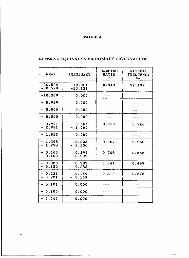
loop discrete system. The s-domain equivalent eigenvalues of the closed-loop lateral system
are shown in Table 4. The singular values for the discrete plant with the loop broken at
the input is shown in Table 5.
The longitudinal/vertical design model state consists of the following twenty compo-
nents:
{V',w,q, O,zr, Wb, Wh, ST, 6e, 6th, ti:, &:, S', itc1,c2, I I , I2, 6thc,6ec}
The longitudinal feedback vector excludes some of the components of the state vector
such as the inertial speed in vertical body axis w', the longitudinal and vertical wind
velocities, the true aircraft altitude, the engine thrust and the elevator surface position.
I 68
On the other hand, the complementary filtered altitude (-;), sink rate and accelerations
are used by the controller, as can be seen by the feedback vector components
In the longitudinal/vertical control law, the commanded variables are predicted vertical
position and airspeed. Thus, the integral of the error in the predicted vertical position
and the airspeed are used in the feedback law. The throttle rate and elevator rate are, the
control components; however, as discussed in Section I1 C, the actual control commands
are the throttle and elevator positions 6thc and 6ec, respectively. The longitudinal/ve'rtical
feedback control structure is summarized in Table 6.
The command design model parameters required for the feedforward control of the
longitudinal/vertical trajectory is summarized in Table 7. The gains designed for the
feedforward and feedback controllers are shown in Table 8.
Closing the loop with the output feedback gains obtained results in the closed-loop
equivalent s-domain eigenvalues shown in Table 9. The singular value, eigenvalue and Bode
plots of the closed-loop system are shown in Figure 4.
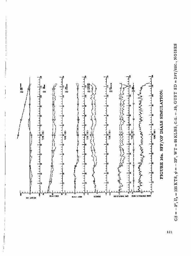
B . NONLINEAR SIMULATION
The performance of the digital automatic landing system described above is evaluated
in this part through a digital computer simulation. The ATOPS B-737-100 aerodynamics,
actuator systems, kinematics, servo, hydraulic and other systems have been simulated in
considerable detail in a nonlinear digital computer simulation. In this simulation, dynamic
systems such as the complementary filter, the yaw damper, the spoiler-aileron coupling,
the engine, etc. are modeled as nonlinear systems which accurately describe their actual
behavior rather than their linearized versions used in the open-loop plant model.
The digital automatic control system described in the preceding sections is simulated
in detail. The control law simulation is then interfaced with the aircraft simulation so that
69
the control commands computed by the design become the input to the aircraft control
actuator systems. Numerous simulations of the closed-loop aircraft system were performed
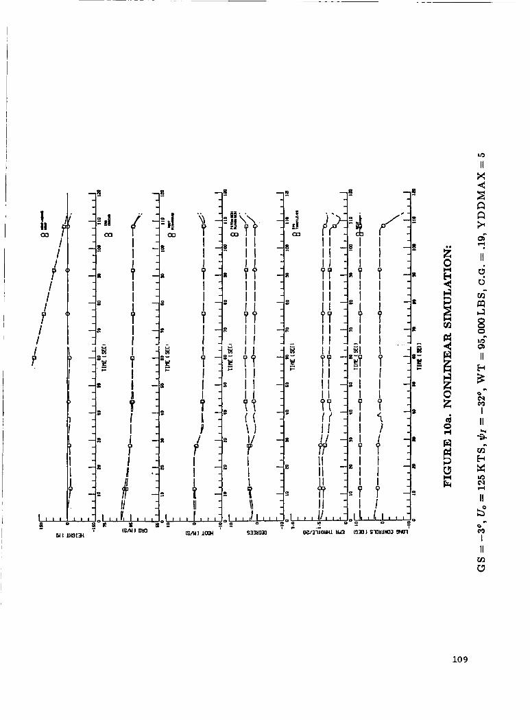
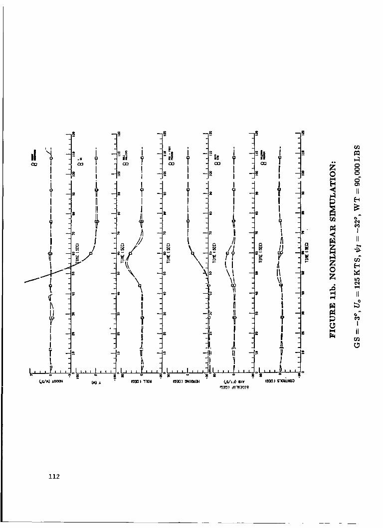
under a variety of different conditions. The aircraft response in simulations are shown in
Figures 5 - 16. The digital control system simulates the incremental implementation shown in Section
11. C Eqs. (129) - (133). While other incremental implementations are possible, they
are not used here. It should be noted that, since both lateral and longitudinal/vertical
controllers designed used a control rate structure, Eq. (133) is, in fact, implemented to
obtain the commands for the aileron, rudder, elevator and throttle positions. The actual
outputs of the control system are the control position commands 6,.
The Boeing 737 aircraft used here has a baseline stabilizer automatic trim logic.
The auto-trim logic drives the stabilizer surface so as to minimize the moment on the
elevator hinge, thus providing maximum authority for the elevator to react to sudden
changes in the flight parameters. The stabilizer movement is much slower than that of
the elevator and does not introduce further dynamic modes in the models. The use of the
incremental implementation is very suitable to accommodate such slow moving surfaces.
In the nonlinear simulations of the automatic landing system designed here, the stabilizer
automatic trim logic is turned on; so that the stabilizer automatically trims the aircraft
even though the plQts shown do not include the stabilizer position.
The control system iteration rate used in the simulation is 10 Hz which is also the
sampling rate used in the control law design. Since the control law is digital, this update
rate must be used for the controller simulation. Hnwever, the sixc!&kz of the ZiiciSt
aerodynamic and on-board systems is performed at 20 Hz. Since these system describe
continuous processes with some modes of high natural frequency, their simulation requires
a higher update rate for accuracy. It is also important to note from Eqs. (129) - (133) that the control system output 6, at time t k uses only variables available at time t k - 1 .
Therefore, as long as the real-time computation of the commands, &, require no more
70
I
than 100 msecs, no computational delay will be present. It is assumed that a sufficiently
fast flight computer will be used to compute the incremental implementation commands.
Thus, the accuracy of the digital control system simulation is expected to be restricted
to round-off errors due to limitations in the word length of the flight computer, possible
mismatches in obtaining exactly a 10 Hz rate, input-output limitations, etc.
The feedforward and feedback control gains used in the simulation are given in Tables
3 and 8. The simulation of the actual commanded path shown by Eq. (132) in the
incremental implementation equations is performed as described in Section 111. It should
be noted that the actual command model uses estimates of the position and of the velocity
of the aircraft c.g.. thus, the feedforward control law implementation actually contains
nonlinear feedback. The coupling is usually rather low and may be neglected. However, a
more complete evaluation should include these feedback effects as well as the effect of the
feedback control law.
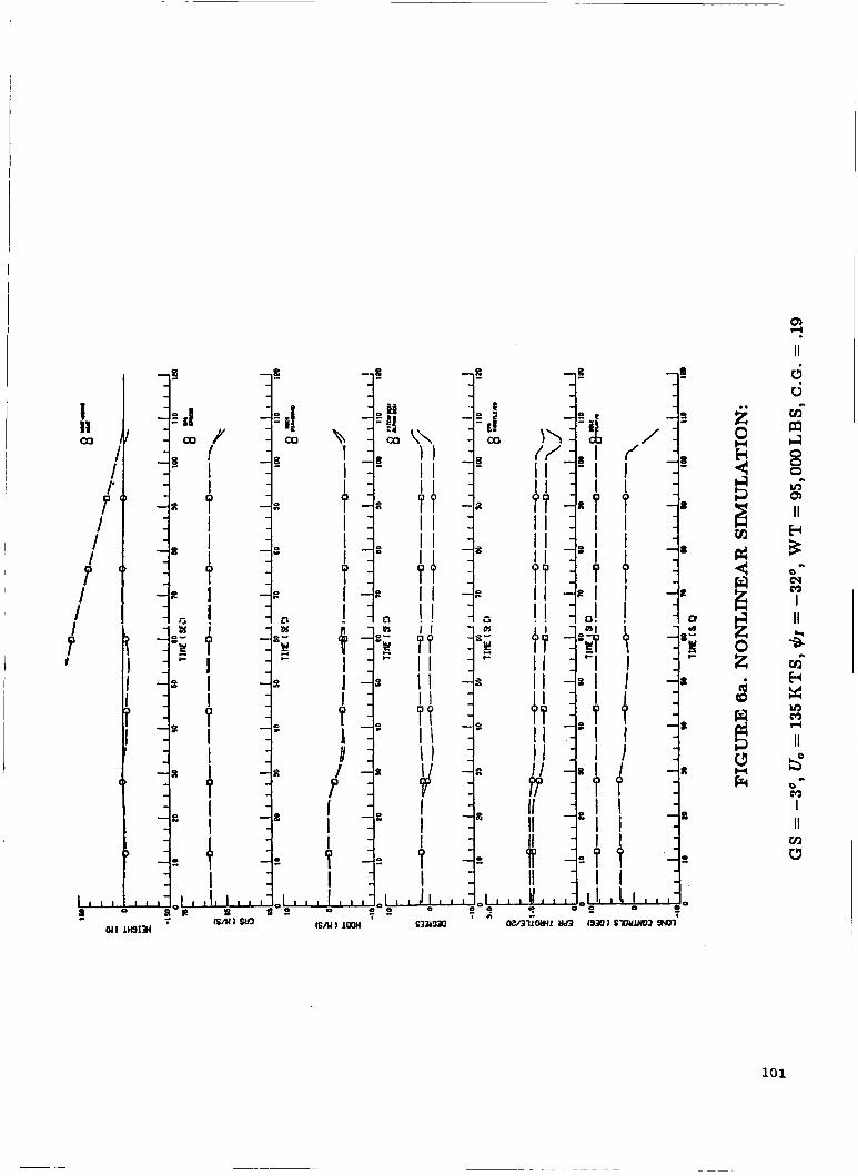
The simulations shown in Figures 5 - 16 are initialized at an estimated altitude of
950 ft. At initialization, the aircraft is flying a constant altitude path with level wings
and a heading so as to intercept the localizer or the runway centerline at some point, X I .
The automatic landing system is engaged at the initialization of the simulation. At that
point, the control law checks to see whether the localizer glideslope capture criteria are
satisfied. The initi-a1 conditions have been selected so that neither the localizer nor the
glideslope capture criterion will be met at this point. Thus, according to the command
path generated, the aircraft continues along the same track angle with level wings and
maintains a constant altitude.
At initialization, the aircraft calibrated airspeed is selected to be 135 knots. On the
other hand, in most of the simulations, the commanded airspeed V, is 125 knots. Accord-
ingly, the control law experiences an instantaneous error of about 10 knots at initialization.
As described in Section 111, the feedforward command model generates a linearly decreasing
airspeed profile from this initial speed to its commanded speed. As seen in the simulations,
71
the aircraft decelerates, following the commanded airspeed, until V, is reached. When the
commanded airspeed V, is 135 knots, as shown in Figure 6, then the initial airspeed error
is zero, and the airspeed command is a constant value of V,. As can bee seen from Figure
6, the control law accurately maintains the commanded speed of 135 knots rather than
reducing it to 125 knots as it does when the commanded airspeed is 125 knots.
As the control law continually tests to see if the glideslope or localizer capture criteria
are satisfied, whether the glideslope or the localizer capture will be the first to engage
depends on the aircraft's position, its heading relative to the runway centerline and the
commanded glideslope angle, with other parameters having generally a lesser effect. In
almost all the simulations shown here, one capture mode is engaged soon after the other,
so that the aircraft flight path is a curved 3D path in both the lateral and vertical planes.
Ability to perform both localizer and glideslope captures simultaneously is described in
order to achieve close-in captures, as it is no longer necessary to perform localizer capture
first and then engage the glideslope capture.
When the desired glideslope angle is 3O, the glideslope capture criterion is satisfied
first in most of the simulations. The initiation of the glideslope capture maneuvers can be
clearly seen in the commanded and actual sink rate plots. Both commanded and actual
sink rate smoothly transition from level flight to the sink rate required to remain on the
desired glideslope at the desired airspeed. Also note the pitch angle and angle of attack
movements during the glideslope capture maneuvers. Whereas the angles coincide when
flying a constant altitude path, when glideslope capture is engaged automatically, the
control law smoothly pitches the aircraft down to capture the glideslope. Note that there
is no initial tendency to pitch in the 5rong" direction.
Also note that prior to glideslope capture, the pitch and angle of attack have to
increase slightly when the aircraft is decelerating in order to compensate for the reduction
of lift due to the airspeed, hence dynamic pressure, reduction. The needed extra lift is
obtained by pitching up and increasing the angle of attack, albeit with lag which results
72
in a small altitude offset. On the other hand, when the aircraft does not decelerate, as
shown in Figure 6, the aircraft pitch and angle of attack remain essentially constant as it
is not necessary to obtain extra lift to maintain altitude.
It should be noted that since maneuvers are principally performed by the feedfor-
ward controller, the glideslope capture performance is an indication that the feedforward
controller is satisfactory for this type of maneuver. Observation of the throttle and eleva-
tor positions shows that the feedforward controller pitches down by initially lowering the
throttle rather than using the elevator. For the B-737 which has a thrust line considerably
lower than the c.g., reducing thrust has the added effect of reducing the pitching moment.
This control strategy is precisely the one that best suits this aircraft, since simply using
the elevator to pitch would have the unwanted result of increasing the airspeed. Thus, the
stochastic feedforward control approach is indeed making use of the plant design model
information aa would be desired.
At the end of the glideslope capture, the altitude error is redefined causing an instan-
taneous move in its value. This causes a corresponding sudden and undesired transient
in the elevator and throttle commands when the altitude error move is appreciable. This
glitch can be removed in a number of ways, including the use of a simple easysn function
at the appropriate time.
It should be noted that the smoothness of the glideslope capture maneuver and its du-
ration are directly related to the parameter lklmaz; i.e., the maximum vertical acceleration
of the commanded altitude profile. By simply varying this parameter at any time prior to
glideslope capture, the commanded capture path may be changed on-line to a smoother
or faster maneuver as desired.
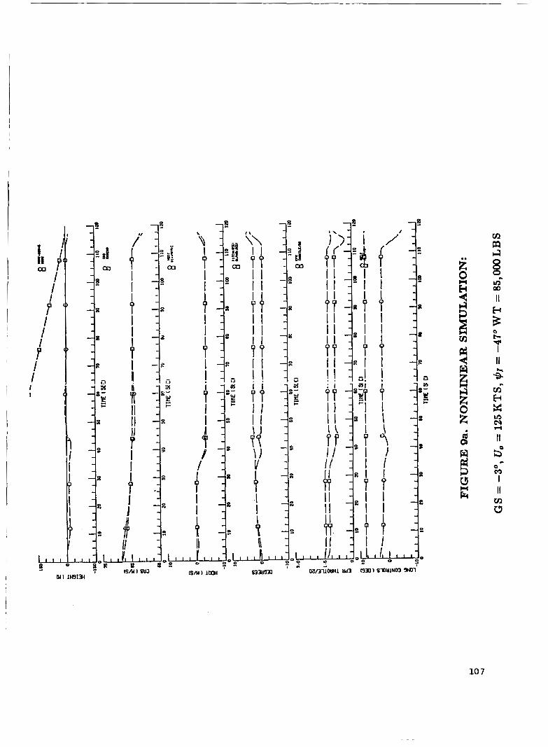
In Figures 7 and 8, the automatic landing system captures steep glideslope of 4' and
4.5', respectively. The glideslope capture path generated by the feedforward model given
in the previous section by Eqs. (234) - (248) is automatically modified to result in a vertical
profile which captures a steeper glideslope, tracks it and flares from this steeper glideslope.
73
Since the same maximum vertical acceleration value is used for all glideslope angles, it may
be noted that the duration of the steeper glideslope captures is slightly longer. However,
the basic characteristics of the response and of the control law remain unchanged.
It should also be noted that the feedforward and feedback control gains remain un-
changed while the commanded vertical path varies according to speed or glideslope angle.
Thus, the feedforward control law tracks the commanded path within the class of com-
manded trajectories. It is clear that if the commanded paths are sufficiently different
from each other, feedforward controllers adapted to the specific characteristics of each
path would result in =better" performance. One such approach would be to extend the
stochastic feedforward approach to include optimal gain scheduling.
In the simulation of the steep glideslope cases, it may be noted that glideslope capture
occurs later. This is a consequence of the geometry, as the initial aircraft altitude is the
same. In the case of the 4' glideslope both localizer and glideslope capture occur in the
same period of time. Localizer capture occurs mostly before the aircraft captures the
steeper 4.5' glideslope in part due to a larger localizer intercept angle of 47". In all cases,
the control law captures the desired glideslope by satisfactorily tracking the commanded
capture path.
When the glideslope capture is performed, the aircraft tracks the desired glideslope
until the flare mode i s engaged. As can be seen from the simulations of different glideslope
angles (i.e., Figures 5 - 8), the aircraft remains on the desired glideslope with essentially
the same precision for shallow and steep glideslopes.
The flare mode is engaged when the flare criterion in Eq. (245) is satisfied. In this
mode, both the flare vertical profile generated as well as the airspeed reduction profile are
commanded. As can be seen from the simulations, the aircraft pitches up increasing its
angle of attack and the lift as desired; this results in a corresponding reduction in the sink
rate and the airspeed until touchdown. This is achieved by using the elevator to pitch up
while lowering the throttle to reduce the airspeed.
74
It can be seen that in all cases, the pitch angle at touchdown is comfortable above
zero and still rising. This pitch attitude at touchdown is necessary to avoid landing on the
nose wheel which is not designed for the high load at touchdown.
As the flare maneuver is significantly sharper than the glideslope capture maneuver,
it requires faster control action. Thus, the measurement noise covariance, pf, for the
command model forcing vector was reduced to obtain the flare gains, resulting in a higher
forcing vector gain, Kf, during flare as shown in Table 8. Due to the complexity of the
flare maneuver and the high accuracy needed in tracking the altitude profile, a higher order
altitude command model would model this profile more accurately.
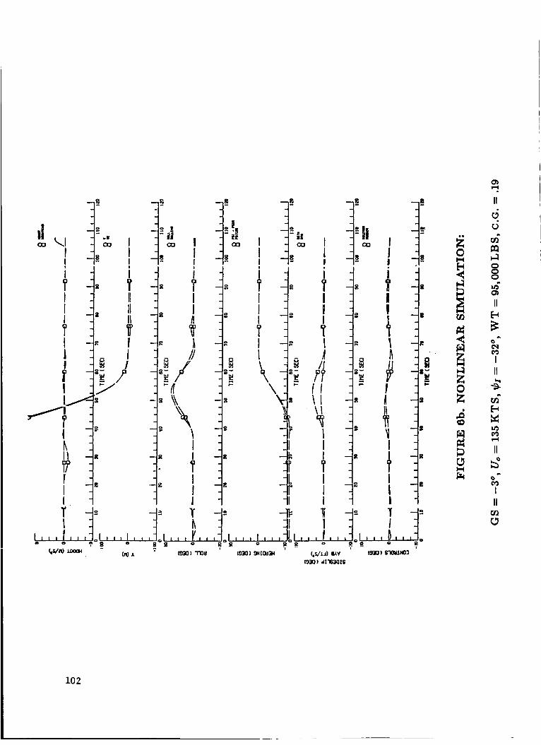
The localizer capture for a 3' glideslope and localizer intercept angle of 32O, as shown
in Figure 5, is initiated near the end of the glideslope capture maneuver. As can be seen
from the heading and roll plots, the aircraft yaw and roll angles track their commanded
trajectories closely and capture the localizer. The lateral position is also seen to track its
commanded profile accurately. Although a small deviation from the localizer is present,
this does not resemble a usual overshoot pattern as it occurs after reaching the localizer.
In all cases, this offset is quite small and tends not to exceed 3 m. As in the case of
the glideslope capture, the high accuracy of the tracking of the lateral position indicates
that the stochastic feedforward controller can produce satisfactory feedforward control law
designs.
During the maneuver, the roll angle and the lateral position commands are selected
so as to produce a coordinated turn when perfect tracking occurs. The sideslip angle plots
indicate that the sideslip angle remains well within 1' of sideslip during the whole final
approach excluding, of course, the decrab maneuver shown in Figure 14. The maximum
sideslip tends to occur during localizer capture slightly after the peak bank angle. On the
other hand, note that the lateral acceleration is plotted on the same set of axes and follows
the roll angle quite closely, as expected during a coordinated turn, whereas the lateral
specific force in the body axes remains near zero in a coordinated turn.
75
The smoothness and duration of the localizer capture path command can be varied
by varying the maximum commanded lateral acceleration Igimcrz. This maximum acceler-
ation is set to 10 f t / s e c 2 in most of the simulations shown. However, Figure 10 shows a
simulation where IClmaz is set to a value of 5 f t / s e c 2 . Observation of the lateral variables
shows that the localizer capture is smoother, lasts longer, requires a lower maximum roll
angle to capture as well as resulting in a lower maximum lateral acceleration as expected.
The turn coordination, although acceptable for IGlmoz value of 10, appears to be improved
as indicated by a lower maximum sideslip angle. The tracking of the lateral position also
shows some improvement. Thus, the feedforward control law can clearly track lateral com-
mand paths where the lateral acceleration does not exceed 10 f t / s e c 2 with no change in
the feedforward control gains.
A number of simulations are shown in Figures 5 - 16 where the sensitivity of the
automatic landing system to various parameters is shown. For example, the aircraft weight
is varied among 85,000 Ibs, 90,000 lbs, and 95,000 Ibs. The center of gravity of the aircraft
is also varied in tandem with the weight. Figures 13 - 16 shows the sensitivity to winds
and noise including bias errors. The wind gust standard deviation used in the simulations
containing gusts is 2 ft/sec. (0.61 m/sec.). The airspeed command is varied between 125
and 135 knots, while the commanded glideslope angles simulated are 3 O , do and 4.5O.
76
V. CONCLUSIONS AND RECOMMENDATIONS
In this study, a combined stochastic feedforward/feedback control design methodology
is developed, and a digital automatic landing system is designed using this approach. It
is considered that the main objective of a control law is to enable the plant to track a
desired or commanded trajectory selected from a given class of trajectories as closely as
possible in the presence of random and deterministic disturbances and despite uncertainties
about the plant. The feedforward controller tries to track the desired or commanded
trajectory, whereas the feedback controller tries to maintain the plant state near the desired
trajectory despite the presence of random, and possibly deterministic, disturbances and
uncertainties about the plant. Modern control theory has concentrated more attention
on the important feedback control problem, while the feedforward control problem has
received less attention.
The feedforward control problem is formulated as a stochastic output feedback prob-
lem where the plant contains unstable and uncontrollable modes. As the standard output
feedback algorithm requires an initial gain which stabilizes the plant, a new algorithm is
developed to obtain the feedforward control gains. The necessary conditions are shown to
result in coupled linear matrix equations, implying that when a solution exists, it is indeed
the globally optimal control gain.
The formulation of the feedforward problem in a stochastic, rather than the standard
deterministic, setting is significant in two ways. First, the class of desired trajectories
from which the actually commanded path is selected can be effectively described as a
random process generated by a dynamical system driven by a white noise process. The
second, and more important, implication of a stochastic optimization formulation is the
tacit understanding that “perfect tracking” is often not possible due to various reasons
including uncertainties about, or variation in the, plant parameters, the presence of plant
77
nonlinearities and unmatched initial conditions. Thus, questions about the robustness and
sensitivity of the feedforward controller arise naturally in this context.
A combined stochastic feedforward/feedback control methodology is developed where
the main objectives of the feedforward and feedback control laws are clearly seen. Fur-
thermore, the inclusion of error integral feedback, dynamic compensation, rate command
control structure, etc. is an integral element of the methodology. Another advantage
of the methodology is the flexibility that a variety of feedback control design techniques
with arbitrary structures may be employed to obtain the feedback controller; these include
stochastic output feedback, multi-configuration control, decentralized control or frequency
and classical control methods.
Finally, a specific incremental implementation is recommended for the combined feed-
forward/feedback controller. Some advantages of this digital implementation are the sim-
plicity of implementation, the fact that trim values are not needed and that problems
such as integrator wind-up can be largely avoided. The closed-loop eigenvalues using this
implementation are shown to contain the designed closed-loop eigenvalues which would re-
sult if an incremental implementation were not used. It is further shown that when using
an incremental implementation, it is advantageous to design the controller with as many
integrators as the number of controls. Using fewer integrators results in marginally stable
eigenvalues of unity, while using more integrators constrains the placement of eigenvalues.
The choice of the same number of integrators as controls is also an intuitively pleasing one.
A digital automatic landing system for the ATOPS Research Vehicle (a Boeing 737-
100) is designed using the stochastic feedforward controller and stochastic output feedback.
The system control modes include localizer and glideslope capture, localizer and glideslope
track, crab, decrab and flare. Using the recommended incremental implementation, the
control laws are simulated on a digital computer and interfaced with a nonlinear digital
simulation of the aircraft and its systems.
In this study, the feedforward controller takes an equal place along the feedback con-
troller in achieving the overall control objective. While the stochastic feedforward/feedback
approach has been successfully developed and applied to a significant problem, some signif-
icant questions and extensions of the problem remain unanswered, and are recommended
for further study and experimentation. Three general areas of study are worthy of further
investigation:
0 the structure of the feedforward controller
0 the robustness and sensitivity of the feedforward controller
0 optimal gain scheduling of the feedforward controller
The structure of the feedback controller considers questions about the role of feedfor-
ward dynamic compensation, the use of the "future values of the desired trajectory" in the
current control command, the use of the full-state feedforward controller when fast flight
computers are available. An argument can be effectively made that since a pilot knows
the future desired trajectory and uses this information in his current control commands,
the optimal feedforward controller should also take advantage of such information.
The uncertainties about complex system parameters and nonlinear effects bring forth
uncertainties about the trajectory which would be tracked when the actual plant parameter
are different than those used in the feedforward design. Since the feedforward controller
does not determine the stability of the closed-loop plant, instability does not generally
result from such mismatching. However, since unsatisfactory performance would generally
result from a high sensitive feedforward law, it is of interest to study measures of robustness
and design methods which incorporate low sensitivity criteria.
In applications where the plant will vary over a wide range of conditions resulting in
large changes in plant model parameters, or in cases where the command model parameter
vary to achieve some objective, it is necessary to adapt the feedforward control gains
according to varying conditions. This can be achieved by extending the optimal gain
scheduling studies to include feedforward controller. Due to the relative simplicity of the
coupled linear necessary conditions, gain scheduling with respect to all the plant parameters
79
rather than a selected few may be feasible. In particular, the feedforward gain of the
command model forcing vector seems extremely appropriate for such application.
80
REFERENCES
I 1. Ogata, K., Modem Control Ennineering, Prentice-Hall, Englewood Cliffs, New Jersey,
1970.
2. Schultz, D. G. and J. L. Melsa, State Functions and Linear Control Systems, McGraw-
Hill, New York, 1967.
3. Anderson, B. D. 0. and J. B. Moore, Linear Optimal Control, Prentice-Hall, Engle-
wood Cliffs, New Jersey, 1971.
I 4. Kwakernaak, H. and R. Sivan, Linear Optimal Control Systems, John Wiley & Sons,
Inc., New York, 1972.
5. Kailath; T., Linear System, Prentice-Hall, Englewood Cliffs, New Jersey, 1980.
6. O’Brien, M. J. and J. R. Broussard, “Feedforward Control to Track the Output of a
Forced Model”, The 17th IEEE Conference on Decision and Control, San Diego, CA,
January 1979. I
I
7. Halyo, N., “Development of a Digital Automatic Control Law for Steep Glideslope
Capture and Flare”, NASA CR-2834, June 1977.
8. Halyo, N. and R. E. Foulkes, ”On the Quadratic Sampled-Data Regulator with Un-
stable Random Disturbances”, IEEE SMC Cos. Proc. 1974 International Conf. on
Syst., Man and Cybern., October 1974.
9. Broussard, J. R., “Extensions to PIFCGT: Multirate Output Feedback and Optimal
Disturbance Suppression”, NASA CR-3968, March 1986.
10. Maybeck, P. S., Stochastic Models. Estimation and Control, Vol. 3, Academic Press,
New York, 1982.
11. Halyo, N. and J. R. Broussard, “A Convergent Algorithm for the Stochastic Infinite-
Time Discrete Optimal Output Feedback Problem”, Proc. 1981 Joint Auto. Control
Conference, Charlottesville, VA, June 1981.
81
12. Halyo, N. and J. R. Broussard, “Investigation, Development, and Application of Opti-
mal Output Feedback Theory, Volume I - A Convergent Algorithm for the Stochastic
Infinite-Time Discrete Optimal Output Feedback Problem”, NASA CR-3828, August
1984.
13. Halyo, N. and J. R. Broussard, “Algorithms for Output Feedback, Multiple Model and
Decentralized Control Problems”, NASA Aircraft Controls Research - 1983, NASA
CP-2296, October 25-27, 1983.
14. Halyo, N., “Flight Tests of the Digital Integrated Automatic Landing System
(DIALS)”, NASA CR-3859, December 1984.
15. Hueschen, R. M., “The Design, Development, and Flight Testing of a Modern-Control-
Designed Autoland System”, American Control Conference, Boston, Massachusetts,
June 1985.
16. Etkin, B., Dynamics of Atmospheric Flinht, John Wiley & Sons, Inc., New York, 1972.
17. Roskam, J., Flight Dynamics of Ripid and Elastic Airplanes, Parts I & 11, Roskam
Aviation and Engineering Corp., 519 Boulder, Lawrence, KS, 1972.
18. Broussard, J. R. and S. T. Stallman, “Modification and Verification of an ACSL
Simulation of the ATOPS B-737 Research Aircraft”, NASA CR-166049, February
1983.
19. Halyo, N. and A. K. Caglayan, “A Separation Theorem for the Stochastic Sampled-
Data LQG Problem”, International J. of Control, Vol. 23, No. 2, February 1976, pp.
20. Security Classif.(of this page) 21. No. of Pages 22. Price Unclassified 126 A0 7
NASA CR-4078 I 4. Title and Subtitle
A Combined Stochastic Feedfornard and Feedback Control Design Methodology with Application t o Autoland Design
7. Author(s)
Ne-un 9. Performing Organization Name and Address
Information & Control Systems, Incorporated 28 Research Drive Hampton, VA 23666
12. Sponsoring Agency Name and Address NatiqnaZ Aeronautics and Space Administration Washzngton, DC 20546
15. Supplementary Notes
3. Recipient's Catalog No.
5. Report Date July 1987
6. Performing Organization Code
8. Performing Organization Report No.
FR 687102 10. Work Unit No.
11. Contract or Grant No.
NASI-26158 13. Type of Report and Period Covered
Contractor Report 14. Sponsoring Agency Code
505- 66- 41 -04
NASA Langley Technical Monitor: Richard M . Hueschen Final Report
16. Abstract
A combined h t o c h a f i c deeddotrwahd and deedback c o ~ o l design rnehtodoLogy A de- ievdoped and a digs au;tomatLc Landing hqhttem dah a Boeing 737 a h m d t
bigned sing t h i ~ approach. h c k t h e commanded ;tnajectony, w h m m t h e deedback conttol law ;thies t o maintain the plant h M e neah Rhe d e s h e d f i a j ec to t y i n the phuence ad din;twLbancu and un- wukirt.tiu about Rhe plant.
The deedborrwahd conttrol law denign LA 6omLLeccted ab a AtochaAa% opa5mization 2nobLem and A imbedded into t h e htochas,i5c ou;tpu;t deedback phoblem whme f i e p l a n t ~ o n t a i n ~ unA&zbLe and uncontnoUable m o d u . A neur d g o h i ; t h m t o compu;te t h e opa5md jeeddommd gain LA d e v d o p e d . A combined deed@utmd/6eedback confirol law d u i g n aethodology A devdoped. iynamic cornpeadon, conakol nate command h f iuc tunu ahe an i n t e g d phA: 06 Rhe aethodology. An inchmentat h p l e m e W o n LA necommended. R e n ~ d 2 ~ on t h e g g e n v h e s 06 ,the implemented vemun designed conahl kkwh m e phuented.
The n t o c h a d c deeddohwatrdldeedback covttrrol me..thodo.togy LA U e d t o design a fig&.~X aLLtoma&k landing hghtem don t h e ATOPS R a e m c h V e k i d e , a Bocing 737-700 ~A~cha&t. The h y h t e m conttrol moden i n d u d e locae ize tr and g f i d a t o p e captwre and trrack, and dlahe t o touchdown. Renub2 06 a d c t a i e e d noMRinem aimLLea,Cion ad t h e f i g d d coM;Drol lawh, actuatoh hyhtema, and ahcha6.t aetrodynmnicn ahe phuented.
The objec t ive ad ,the deed6o-d c o n h o l law LA t o
l n tk in apphoach, t h e ~ ~ c l e 06 m o h inte5ha.l deedback,
i i . Ke -w*oras (au gested by Authors s)) - e e d [ o m d &nt t ro l , Fedback Cont t to l ,
dethodolog y, 0u;tpUR: Feedback, VigLtd :on.ttol, O p t u n a X CoM;Drol, lncnementae. [ rnplemeWoi i , AuAomatLc Landing, ATOPS, l l A L S
XtcchLx&ti.c Canttrot, c o m a e L c u v u i g n
18. Distribution Statement
Unclassified - Unlimited
Subject Category 63
For sale by the National Technical Information Service, Springfield, Virginia 22161 - NASA-Langley. 1987