A Comparison of the SPOT and Landsat l he ma tic Mapper Satellite Systems for Detecting ~ y p s y Moth Defoliation in Michigan Peter E. Joria and Sean C. Ahearn* University of Minnesota, Remote Sensing Laboratory, 1530 N. Cleveland Ave., St. Paul, MN 55108 Michael Connor USDA Forest Service, Forest Pest Management, 1992 Folwell Avenue, St. Paul, MN 55108

ABSTRACT: The task of monitoring gypsy moth defoliation is becoming more difficult as the area of defoliation increases. The gypsy moth is now established throughout much of the northeastern U.S. and in Michigan, the site of this study. Defoliation in Michigan occurred on over 120,000 hectares in 1989, with a larger area anticipated for 1990. It is imperative that a monitoring system be able to collect information over thgse increasingly larger areas in a short time period and at relatively frequent intervals. In this paper we examine and compare two satellite systems-SPOT and the Landsat Thematic Mapper-for their efficacy in discriminating two levels of defoliation, moderate and severe, and non-defol- iation. This comparison is done with the aid of a forestlnon-forest mask to reduce the confusion between defoliated areas and non-forested areas. An interpretation of optical bar photography and limited ground data were used as reference. Comparisons were made by calculating the probable overlap among the three classes (severe, moderate, and non-defoliated) using Mahalanobis distance, and with supervised and unsupervised classifications. Results indicated that Landsat TM provided greater separability of the three classes. The Landsat TM classification had an 82 percent agreement with the reference data used in the study.

INTRODUCTION

HE GYPSY MOTH (Lymantria dispar L.) is the most significant Tdefoliator of hardwood trees in the northeastern U.S. Since its introduction to Massachusetts from Europe in 1869, the in- sect has been spreading at an increasing rate, and is just now reaching the more susceptible oak-pine and oak-hickory forests of the eastern United States (Cameron, 1986). Populations now exist in several northwestern states, but the insect is well es- tablished throughout the northeastern U.S. and in Michigan, the site of this study.

Defoliation in Michigan has increased dramatically during the past decade. In the last several years alone, aerial surveys in- dicate an increase in defoliation from 16,000 hectares in 1987 to nearly 120,000 hectares in the summer of 1989. With close to 5 million hectares in Michigan considered susceptiile to the gypsy moth, it is likely that defoliation will reach several hundred thousand hectares annually (Montgomery, 1988).

As the extent of annual damage increases, so will the de- mands placed on monitoring systems. These systems should be able to (1) provide a synoptic view over a large area; (2) provide several opportunities for data acquisition within a brief biological window (to avoid problems with cloud cover or haze); and (3) provide suitable accuracy at a reasonable cost. High altitude photography and satellite images are possible solutions in that they are able to gather data quickly over large areas at minimal cost. Digital satellite images offer the added benefit of compatibility with Geographic Information Systems (GIs), facil- itating analysis and revision. This study compares two satellite systems, SPOT and the

Landsat Thematic Mapper (TM), for monitoring forest defolia- tion caused by the gypsy moth over a 200 krn2 area in central Michigan. The comparison is based on the satellite sensors' abil- ity to accurately identify areas of defoliation and separate these according to the severity of the damage.

High-altitude, optical bar camera (OK) photography was in-

*Presently with the Department of GeologyIGeography, Hunter Col- lege, New York, NY 10021

PHOTOGRAMMETRIC ENGINEERING & REMOTE SENSING, Vol. 57, No. 12, December 1991, pp. 1605-1612.

cluded in the study as a reference source. Interpretation of the OBC photography was first compared to ground plots in order to judge its reliability. It was then used as a more extensive "ground truth" for a second-level comparison between the two satellite images.

DEFOLIATION MONITORING TECHNIQUES Sketch mapping is perhaps the most common method used

for monitoring extensive forest damage. Results from this tech- nique are often subjective due to differences among interpreters in experience and ability to quickly identify (and locate on maps) defoliation of varying intensity on the ground (Talerico et al., 1978; Turner, 1984). In addition, the utility of low-altitude mon- itoring techniques may be limited by the changes that occur in the forest canopy during the time required for surveillance over increasingly larger areas (Williams, 1975). Detection of damage caused by the gypsy moth is best performed when defoliation has reached its peak in most areas and before severely defol- iated trees start to re-leaf. This may be an interval of perhaps two or three weeks, while the ground coverage required may exceed several million hectares.

Satellites have been used to detect forest damage since the early 1970s. Rohde and Moore (1974) analyzed single and multi- date Landsat-1 composites for a gypsy moth defoliation study in Pennsylvania. Confusion of areas of defoliation with agri- cultural fields or mining areas, due to the extensive loss of green biomass in severely defoliated stands, was resolved using change detection (multi-date composites). Williams et al. (1979) used a forestlnon-forest mask, derived from an earlier Landsat image depicting healthy forest conditions, to remove non-forested areas from consideration. The workers still reported confusion of moderate defoliation with healthy forests on northwest slopes, despite the use of band ratios to minimize aspect effects. Nelson (1981) reported moderate defoliation to be indistinguishable from healthy forests (at a classification resolution of 320 by 220 m), while heavy defoliation was distinct throughout a five-week temporal window.

By 1983, a three-year joint project between NASA's Goddard Space Flight Center and the Pennsylvania Bureau of Forestry,

0099-1112/9V5710-1605$03.00/0 01991 American Soaety for Photogrammetry

and Remote Sensing

PHOTOGRAMMETRIC ENGINEERING & REMOTE SENSING, 1991

Division of Forest Pest Management, had resulted in an auto- mated defoliation assessment system (Dottavio and Williams, 1983; Williams and Stauffer, 1978). A total of four georeferenced database layers were combined in a GIs: (1) a Landsat mosaic of Pennsylvania depicting healthy forest conditions; (2) a forest1 non-forest binary mask developed from layer (1); (3) a Landsat mosaic depicting defoliation for the current year; and (4) county and forest pest management boundaries. If cloud cover were to eliminate Landsat coverage for a particular year, aerial sketch mapping would serve as a backup, with the results later digi- tized and entered into the database.

Some limitations of the Landsat technology commonly cited in these early studies were its poor spatial resolution (79 m) and infrequent overpasses (an 18-day cycle). With the successful launchings of Landsats-4 and -5 in the early 1980s and SPOT-lin 1986, researchers had access to images with higher resolution, better spectral characteristics (including mid-IR bands), and shorter repeat cycles.

Vogelmann and Rock (1988) found the Landsat RYI mid-IR bands, which are sensitive to leaf moisture content, to be useful in assessing conifer forest decline in Vermont and New Hamp- shire. Results from 30-m resolution TM data were similar to those obtained with Thematic Mapper Simulator (ms) data at 16- to 17-m resolution.

Ciesla et al. (1989) manually interpreted SPOT-I color compos- ites for a study of gypsy moth defoliation in southcentral Penn- sylvania and western Maryland. Confusion of fallow fields and talus slopes with heavy defoliation again indicated the value of a preliminary foresvnon-forest mask. Conifer plantations, shaded slopes, and a large degree of mortality in some stands were sources of confusion with moderate defoliation. The researchers concluded that SPOT color composites provdied adequate re- sults at a regional or statewide scale, but were unacceptable for more specific assessments such as effectiveness of spray pro- grams.

Lessons learned from this earlier research were incorporated into our comparison of the latest generation Earth resources satellites. These included development of a binary (foresvnon- forest) mask to eliminate some potential sources of confusion, and digital analysis of the SPOT and RYI satellite images to take full advantage of the spectral and radiometric data, while min- imizing subjectivity in the classifications.

METHODS

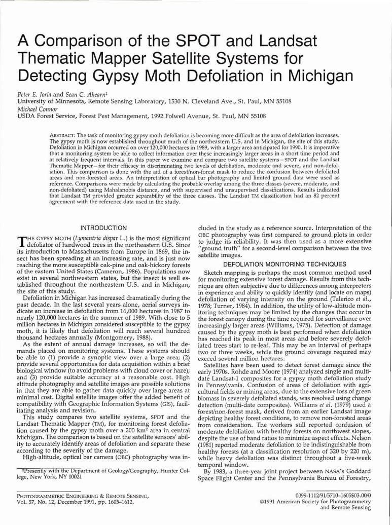
A 6000 km2, four-county area in Michigan was initially chosen for study, but a cloud-free subset (200 km2) of this area was ultimately used in the comparison (Figure 1). Second- and third- growth forests cover slightly more than half of the subset area. Oak species dominate most of the upland and sandier soils in the area, with maple and aspen as stronger components on the more mesic sites.

Data were from four different sources: a full SPOT scene (60 by 60 km); a Landsat Thematic Mapper "moveable" scene (100 by 100 km); OBC photography for all four counties; and 17 ground plots. All data were acquired between the last week of June and the second week of July, 1988, at the peak of defoliation for the study area.

A 27 June 1988 SPOT scene (ID# 16032618806271640512X), centered at 43'47'N 84'38'W, was used, though cloud cover and haze ranged from 10 to 25 percent for two quadrants of the scene. No clearer scenes were available for the period of 20 June- 20 July 1988. The Thematic Mapper scene (ID# 5158115523), centered at 43"501N 84"35'W, was acquired on 29 June 1988. Cloud cover in the scene was less than 10 percent.

Optical bar photography was taken at mid-day on 5 July 1988.

MICHIGAN

FIG. 1. Study area in northeast Clare and northwest Gladwin Counties.

Flight lines were approximately 29 km apart, with 60 percent overlap at nadir. Cloud cover was less than 10 percent within 18 km of the fight path. The camera (ITEK IRIS 11) was mounted in an ER-2 reconnaissance aircraft flying at an altitude of ap- proximately 20 km AMSL. Photo scale was 1:32,500 at nadir. The photography was acquired as part of a continuing gypsy moth project, begun in 1984, involving NASA and the USDA Forest Service, State and Private Forestry, for the Northeastern Area.

Ground plots were established between 5 and 12 July 1988. Each consisted of three variable-radius subplots. Subplot mea- surements were (1) DBH of all trees greater than 2 inches, (2) species, (3) canopy layer, and (4) percent of crown defoliated. Stands were considered severely defoliated if 75 percent or more of the measured trees were 75 percent or more defoliated, while moderate defoliation was indicated by 50 percent or more de- foliation on 50 percent or more of the trees. Defoliation below these levels was categorized as non-defoliated. These defini- tions were chosen in order to remain consistent with classifi- cations by the Michigan Department of Natural Resources (DNR). Collection of ground data came to an end when increasing oc- currences of re-leafing among severely defoliated trees made it too difficult to discriminate between these secondary leaves and the primary leaves of non-defoliated trees.

The SPOT and TM scenes were delivered in a computer-com- patible tape (CcT) format and were digitally analyzed. The oBc photography was manually interpreted, with the interpretation transferred onto USGS maps before being converted to a digital format.

Supervised and unsupervised classifications were performed on both satellite images. A spatial clustering approach was used, based on a modified SEARCH algorithm, for input into a Baye- sian maximum-likelihood classifier (Ahearn and Lillesand, 1986; NASAIERL, 1981). Unsupervised classifications used pixel counts for each cluster, divided by the total number of pixels sampled during the cluster building stage, as estimates (prior probabil- ities) of that class in the entire subset. Further processing, in- cluding majority and boundary filters, overlays, and accuracy assessments, were performed using ERDAS, a raster-based GIs and image processing package.

DETECTING GYPSY MOTH DEFOLIATION

Manual interpretation of the optical bar photography was performed by the USDA Forest Service, State and Private For- estry, for the Northeastern Area. The film was viewed mon- oscopically on a light table, and areas of moderate or severe defoliation were outlined. The resulting polygons were visually transferred onto 7.5 minute maps (1:24,000 or 1:25,000 scale). These maps were then digitized using pcARC/INFO. Portions of this coverage were converted into raster formats compatible with the satellite imagery (i.e., 30- by 30- or 20- by 20-m pixels).

Extensive cloud cover, combined with the small number of ground plots, made it impossible to use the ground plots for both training and testing purposes. Instead, we decided upon a two-tiered approach to reference data: (1) accuracy of the OBC interpretation would be assessed by comparison with the 17 ground plots; and (2) the OBC interpretation would serve as a reference layer for a relative comparison of the SPOT and TM images, using a cloud-free subset from each. The area chosen encompasses approximately 200 km2 in northern Clare and Gladwin counties, and contains extensive examples of each de- folation category.

High altitude photography has been used as reference data in other studies of satellite imagery, though the practice is far from ideal (Ciesla et al., 1989; Dottavio and Williams, 1983; Nel- son, 1981; Williams et al., 1979). The comparison with ground plots provides some indication of the reliability of the OBC inter- pretation and allows use of all 17 plots for testing purposes alone (Table 1).

The SPOT and TM subscenes were geometrically corrected and transformed to the Universal Transverse Mercator (UTM) coor- dinate system using a nearest-neighbor resampling scheme and an RMS error of less than one pixel.

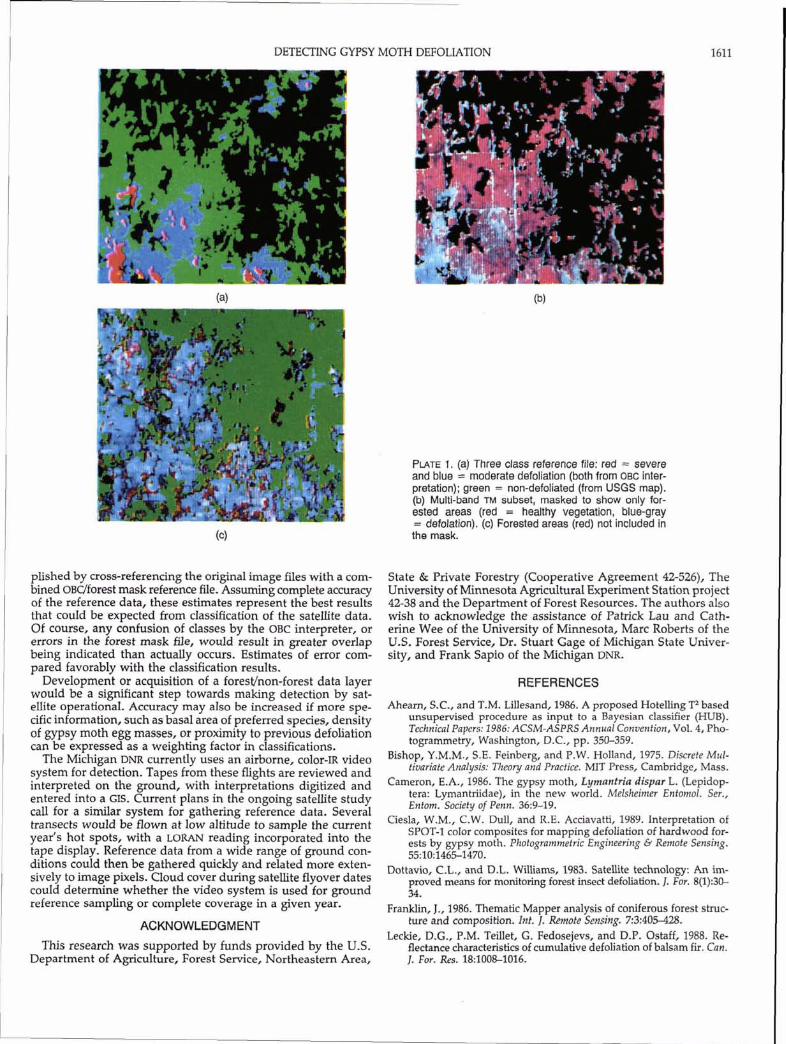
A foresthon-forest mask for the subset area was developed to eliminate non-forested areas from consideration. Because the OBC interpretation only included moderately or severely defol- iated forests, we needed an additional source for healthy for- ests. Forested areas delineated on USGS maps (1:100,000 scale) were digitized and transformed into 20-m and 30-m resolution raster files. The OBC file was then overlaid on this file to produce a three-class "reference" file that identified "severe," "moder- ate," and "non-defoliated areas within the study subset (Plate

Optical Ground Plots Bar Severe Moderate Non-Defol Totals

Severe 2 0 0 0 Moderate 3 5 1 9

Non-Defol 0 1 5 6 Totals 5 6 6 17

Overall Accuracv: 70.59%

'Diagonal valuedtotal.

la). The reference file was then applied as a mask to each of the original multi-band images, producing "forest only images (Plate lb).

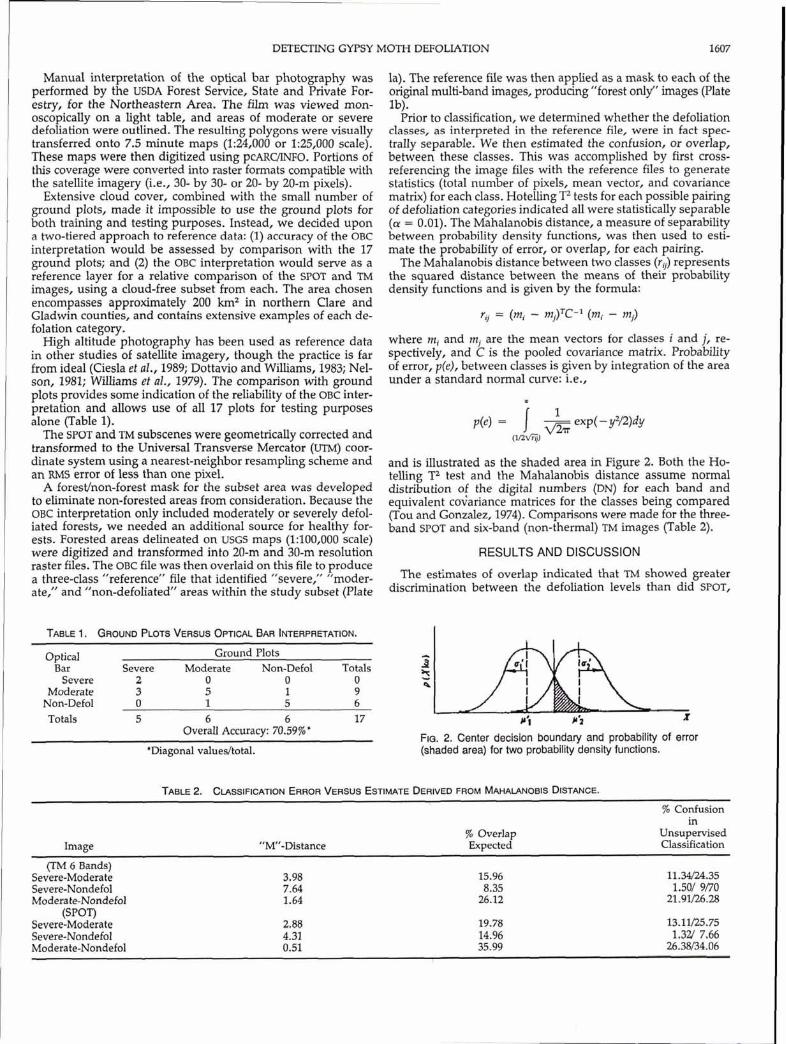
Prior to classification, we determined whether the defoliation classes, as interpreted in the reference file, were in fact spec- trally separable. We then estimated the confusion, or overlap, between these classes. This was accomplished by first cross- referencing the image files with the reference files to generate statistics (total number of pixels, mean vector, and covariance matrix) for each class. Hotelling T2 tests for each possible pairing of defoliation categories indicated all were statistically separable (a = 0.01). The Mahalanobis distance, a measure of separability between probability density functions, was then used to esti- mate the probability of error, or overlap, for each pairing.

The Mahalanobis distance between two classes (rV) represents the squared distance between the means of their probability density functions and is given by the formula:

r, = (m, - mj)TC-l (mi - mj)

where mi and mi are the mean vectors for classes i and j, re- spectively, and C is the pooled covariance matrix. Probability of error, p(e), between classes is given by integration of the area under a standard normal curve: i.e.,

and is illustrated as the shaded area in Figure 2. Both the Ho- telling T2 test and the Mahalanobis distance assume normal distribution of the digital numbers (DN) for each band and equivalent covariance matrices for the classes being compared (Tou and Gonzalez, 1974). Comparisons were made for the three- band SPOT and six-band (non-thermal) TM images (Table 2).

RESULTS AND DISCUSSION

The estimates of overlap indicated that TM showed greater discrimination between the defoliation levels than did SPOT,

FIG. 2. Center decision boundary and probability of error (shaded area) for two probability density functions.

TABLE 2. CLASSIFICATION ERROR VERSUS ESTIMATE DERIVED FROM MAHALANOBIS DISTANCE. % Confusion

in % Overlap Unsupervised

Image "M-Distance Expected Classification -

(TM 6 Bands) Severe-Moderate Severe-Nondefol Moderate-Nondefol

(SPOT) ~everd-~odbate Severe-Nondefol Moderate-Nondefol

PHOTOGRAMMETRIC ENGINEERING & REMOTE SENSING, 1991

with the greatest spectral overlap occuring between moderate and non-defoliated information classes.

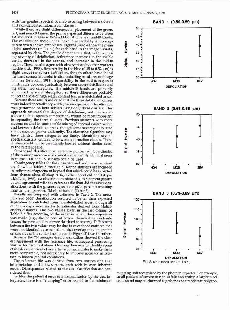
While there are slight differences in placement of the green, red, and near-IR bands, the primary spectral difference between TM and SPOT images is TM'S additional blue and mid-IR bands. The contribution these bands make to separability is more ap- parent when shown graphically. Figures 3 and 4 show the mean digital numbers (+ 1 s.d.) for each band in the image subsets, separated by class. The graphs demonstrate that, with increas- ing severity of defoliation, reflectance increases in the visible bands, decreases in the near-IR, and increases in the mid-R region. These results agree with observations by other workers (Leckie et al., 1988). Separability in the blue (0.45 to 0.52 km) is slight except for severe defoliation, though others have found the band somewhat useful in discriminating basal area or foliage biomass (Franklin, 1986). Separability in the mid-IR region is much more obvious, particularly between severe defoliation and the other two categories. The middle-IR bands are primarily influenced by water absorption, so these differences probably reflect the loss of high water content leaves in defoliated areas.

Because these results indicated that the three defoliation classes were indeed spectrally separable, an unsupervised classification was performed on both subsets using only three clusters. This approach assumed that degree of defoliation, not another at- tribute such as species composition, would be most important in separating the three clusters. Previous attempts with more clusters resulted in considerable mixing of spectral classes within and between defoliated areas, though some severely defoliated stands showed greater uniformity. The clustering algorithm may have divided these categories too finely, identifying several spectral clusters within and between information classes. These clusters could not be confidently labeled without similar detail in the reference file.

Supervised classifications were also performed. Coordinates of the training areas were recorded so that nearly identical areas from the SPOT and TM subsets could be used.

Contingency tables for the unsupervised and the supervised are shown as Tables 3 through 6. Kappa statistics are included as indicators of agreement beyond that which could be expected from chance alone (Bishop et al., 1975; Rosenfield and Fitzpa- trick-Lins, 1986). TM classifications showed 4 to 8 percent greater overall agreement with the reference file than did the SPOT clas- sifications, with the greatest agreement (67.4 percent) resulting from an unsupervised TM classification (Table 6).

Results are compared with estimates in Table 2. The unsu- pervised SPOT classification resulted in better than expected separation of defoliated from non-defoliated areas, though all other overlaps were similar to estimates derived from Mahal- anobis distances. The two values given in the last column of Table 2 differ according to the order in which the comparison was made (e.g., the percent of severe classified as moderate versus the percent of moderate classified as severe). Differences between the two values may be due to covariance matrices that were not identical as assumed, so that overlap may be greater on one side of the center line (shown in Figure 3) than the other.

Because the TM unsupervised classification showed the clos- est agreement with the reference file, subsequent processing was performed on it alone. Our objective was to identify some of the discrepancies between the two files in order to make them more comparable, not necessarily to improve accuracy in rela- tion to known ground conditions.

The reference file was derived from two sources (the OBC interpretation and a USGS map), each with its own inherent errors. Discrepancies related to the OBC classification are con- sidered first.

Besides the potential error of misclassification by the OBC in- terpreter, there is a "clumping" error related to the minimum

BAND 1 (0.50-0.59 pm) 50

MOD

DEFOLIATION

BAND 2 (0.61-0.68 pm)

I

MOD

DEFOLIATION

BAND 3 (0.79-0.89 pm)

DEFOLIATION FIG. 3. SPOT mean DNS (2 1 s.d.).

mapping unit recognized by the photo interpreter. For example, small pockets of severe or non-defoliation within a larger mod- erate stand may be clumped together as one moderate polygon.

DETECTING GYPSY MOTH DEFOLIATION

BAND 1 (0.45-0.52 km)

s v DEFOLIATION

BAND 3 (0.63-0.69 pm)

DEFOLIATION

BAND 5 (1.55-1.75 pm)

80 - 70 : 1

MN I

MOD I

SN DEFOLIATION

BAND 2 (0.52-0.60 pm) 45 -, 1

25 ! I I I I

MN MOD SEV

OEFOLlATlON

FIG. 4. TM mean DNS ( 2 1 s.d.).

BAND 4 (0.76-0.90 pm) -,

75 ! I I I

MN MOD SEV DEFOLIATION

BAND 7 (2.08-2.35 pm)

I I 1 I

MN MOD SRI DEFOLIATION

Less than 1 percent of the polygons outlined by the OBC inter- OBC interpretation, with the central pixel in the window given preter were smaller than 8100 m2, comparable to a 3 by 3 square a class value equal to that of the plurality of the surrounding of pixels at TM resolution. We used a 3 by $pixel window to pixels. Use of the filter resulted in a nearly 4 percent increase "generalize" the l'M classified image to the resolution of the in overall agreement (71.0 percent).

PHOTOGRAMMETRIC ENGINEERING & REMOTE SENSING, 1991

TABLE 3. SPOT SUPERVISED CLASSIFICATION VERSUS REFERENCE TABLE 5. TM SUPERVISED CLASSIFICATION VERSUS REFERENCE FILE. FILE.

Comm. Comm. Optical Bar Interpretation (Reference) E,

Optical Bar Interpretation (Reference) Err Severe Moderate Non-Defol Totals (%) Severe Moderate Non-Defol Totals (%)

Severe 3095 2012 7178 12285 74.81 Severe 7406 6213 14099 27718 73.28 Moderate 1586 15736 20731 38053 58.65

Moderate 3349 33610 58657 95616 64.85 Non-Defol 201 6335 59567 66103 9.89 Non-Defol 198 14471 122306 136975 10.71 ~~~~l~ (pixels) 4882 24083 87476 116441

Totals (Pixels) 10953 54294 195062 260309 Omm. Error (%) 36.60 34.66 31.90 Omm. Error (%) 32.38 38.10 37.30 Kappa ( X 100): 59.08 48.52 26.20 34.85 Kappa ( X 100): 63.76 39.79 21.28 28.98 Overall Agreement (%): 67.33

Overall Agreement (%): 62.74

TABLE 6. TM UNSUPERVISED CLASSIFICATION VERSUS REFERENCE TABLE 4. SPOT UNSUPERVISED CLASSIFICATION VERSUS REFERENCE FILE.

FILE.

Severe Moderate

Non-Defol Totals (Pixels) Omm. Error (%) Kappa ( x 100):

Comm. Optical Bar Interpretation (Reference) E,.

Severe Moderate Non-Defol Totals (%)

27.07 39.49 41.72 69.40 35.02 17.83 25.36

Overall Agreement (%): 59.36

Comm. Optical Bar Interpretation (Reference) E,

Severe Moderate Non-Defol Totals (%)

Severe 3620 2732 8483 14835 75.60 Moderate 1189 15022 19164 35375 57.53

Non-Defol 73 6329 59829 66231 9.67 Totals (Pixels) 4882 24083 87476 116441 Omm. Error (%) 25.85 37.62 31.61 Kappa (x 100): 70.38 45.96 26.70 35.37

Overall Agreement (%): 67.39

TABLE 7. TM UNSUPERVISED CLASSIFICATION (FILTER AND BOUNDARIES) VERSUS REFERENCE FILE.

There are a number of errors inherent in the digitized USGS laver, the most simificant due to inaccuracies of the orininal map: Some of thele are obvious when the layer is placed<ver Comm.

Optical Bar Interpretation (Reference) E, the TM multi-band image (Plate lc). The amount of forested area (red areas indicating high near-IR reflectance) not covered by Severe Moderate Non-Defol Totals (76) the green mask is considerable, most likely due to growth in Severe 2725 894 2851 6470 57.88 vegetation since the map was last updated.-What can't be seen Moderate 479 10473 5222 16174 35.25 is the amount of forest removed since the map inventory, but Non-Defol 19 3434 49368 52821 6.54 still considered forested in the reference file. This may also be Totals (pixels) 3223 14801 57441 75465 simificant. resulting: in confusion between areas classified as Omm. Error (%) 15.45 29.24 14.05 "dYefoliated in the "TM file and non-defoliated in the reference Kappa ( X 100):' 83.10 62.78 53.16 59.45 file. This is evident in all contingency tables, where a large Overall Agreement (76): 82.91 number of "non-defoliated reference pixels are classified as severe while few "severe" reference pixels are classified as non- defoliated.

Other potential errors in the USGS file relate to registration and digitization. Forest (green) polygons on the original USGS map were outlined using a 0.5-mm lead pencil before being digitized. At the scale of the maps (1:100,000), the effective bor- der ("margin" of error) for these polygons amounts to 50 m on the ground, nearly two TM pixels wide. Conversion from vector to raster format probably added slightly to this error. Minor registration errors also likely resulted from geometric correction and resampling of the original image pixels. Many of the severe defoliation pixels in the classified images occur along the edges of the mask polygons. It is likely that these represent non-for- ested areas on the forest fringe that were included due to in- accuracies of the borders. Roads that were borders between forested areas were also included in the mask and likewise were classified as severe defoliation. In order to remove these from consideration, a one pixel border around each polygon was masked out.

Application of the border to the majority-filter file increased overall agreement to nearly 83 percent (Table 7). While the bor- der reduced the total number of pixels considered by 35 percent,

it decreased the number of non-defoliated pixels classified as severe by 62 percent, indicating that border "severe" pixels were indeed a primary source of error.

CONCLUSION AND SUGGESTIONS FOR IMPROVEMENT

We examined the utility of two forms of satellite imagery (SPOT and the Landsat Thematic Mapper) for detecting defol- iation by the gypsy moth in a 200 krn2 area in central Michigan. Post-classification processing of the TM data resulted in an over- all agreement of 82.9 percent with a reference file. TM agree- ments were approximately 4 percent higher than for SPOT using a supervised approach and 8 percent better using an unsuper- vised approach.

Cloud cover during the SPOT acquisition date limited the size of the area that could be compared, while insufficient ground information required the use of high altitude photography (the Optical Bar Camera) for reference rather than inclusion in the comparison.

The statistical separability and percent overlap of defoliation classes were estimated prior to classification. This was accom-

DETECTING GYPSY MOTH DEFOLIATION

m

plished by moss-referencing the original image files with a com- bined o~C/forest mask reference file. Assuming complete accuracy of the reference data, these estimates represent the best results that could be expected from classification of the satellite data. Of course, any confusion of classes by the OBC interpreter, or errors in the forest mask file, would result in greater overlap being indicated than actually occurs. Estimates of error com- pared favorably with the classification results.

Development or acquisition of a forestlnon-forest data layer would be a significant step towards making detection by sat- ellite operationaI. Accuracy may also be increased if more spe- cific information, such as basal area of preferred species, density of gypsy moth egg masses, or proximity to previous defoliation can be expressed as a weighting factor in classifications.

The Michigan DNR currently uses an airborne, color-IR video system for detection. Tapes from these flights are reviewed and interpreted on the ground, with interpretations digitized and entered into a GIs. Current plans in the ongoing satellite study call for a similar system for gathering reference data. Several transects would be flown at low altitude to sample the current year's hot spots, with a LORAN reading incorporated into the tape display. Reference data from a wide range of ground con- ditions could then be gathered quickly and related more exten- sively to image pixels. Cloud cover during satellite flyover dates could determine whether the video system is used for ground reference sampling or complete coverage in a given year.

ACKNOWLEDGMENT This research was supported by funds provided by the U.S.

Department of Agriculture, Forest Service, Northeastern Area,

PLATE 1. (a) Three class reference file: red = severe and blue = moderate defoliation (both from OBC inter- pretation); green = non-defoliated (from USGS map). @) Multi-band TM subset, masked to show only for- ested areas (red = healthy vegetation, blue-gray = defolatlon). (c) Forested areas (red) not included In the mask.

State & Private Forestry (Cooperative Agreement 42-526), The University of Minnesota Agricultural Experiment Station project 42-38 and the Department of Forest Resources. The authors also wish to acknowledge the assistance of Patrick Lau and Cath- erine Wee of the University of Minnesota, Marc Roberts of the U.S. Forest Service, Dr. Stuart Gage of Michigan State Univer- sity, and Frank Sapio of the Michigan DNR.

REFERENCES

Ahearn, S.C., and T.M. Lillesand, 1986. A proposed Hotelling F based unsupervised procedure as input to a Bayesian classifier (HUB). Technical Papers: 1986: ACSM-ASPRS Annual Convention, Vol. 4, Pho- togrammetry, Washington, D.C., pp. 350359.

Bishop, Y.M.M., S.E. Feinberg, and P.W. Holland, 1975. Discrete Mul- tivariate Analysis: Theory and Practice. MIT Press, Cambridge, Mass.

Cameron, E.A., 1986. The gypsy moth, Lymantria dispar L. (Lepidop- tera: Lymantriidae), in the new world. Melsheimpr Entomol. Ser., Entom. Society of Penn. 369-19.

Ciesla, W.M., C.W. Dull, and R.E. Acciavatti, 1989. Interpretation of SPOT-1 color composites for mapping defoliation of hardwood for- ests by gypsy moth. Photogrammetric Engineering b Remote Sensing. 55:10:1465-1470.

Dottavio, C.L., and D.L. W i , 1983. Satellite technology: An im- proved means for monitoring forest insect defoliation. J. For. 8(1):30- 34.

Franklin, J., 1986. Thematic Mapper analysis of coniferous forest struc- ture and composition. Int. J. Remote Sensing. 7:3:405-428.

Leckie, D.G., P.M. Teillet, G. Fedosejevs, and D.P. Ostaff, 1988. Re- flectance characteristics of cumulative defoliation of balsam fir. Can. J. For. Res. 18:1008-1016.

PHOTOGRAMMETRIC ENGINEERING & REMOTE SENSING, 1991

Montgomery, B.A. (editor), 1988. Gypsy Moth in Michigan 1987. Ext. Bull. E-2142, Cooperative Ext. Sew., Michigan State Univ.

NASAlERL, 1981. ELAS Earth Resources Laboratory Applications Software, NSTL Rept. 183, National Space Technology Laboratory.

Nelson, R.F., 1981. Defining the temporal window for monitoring forest canopy defoliation using LANDSAT. Proc. American Society of Pho- togrammetry 47th Ann. Meet., Washington D.C.

Rosenfield, G.H., and K. Fitzpatrick-Lins, 1986. A coefficient of agree- ment as a measure of thematic classification accuracy. Photogram- metric Engineering & Remote Sensing. 52:2:22%227.

Rohde, W.G., and H.J. Moore, 1974. Forest defoliation assessment with satellite imagery. Proc. 9th Int. Symp. Remote Sens. Env., Univ. of Mich. pp. 1089-1104.

Talerico, R.L., J.E. Walker, and T.A. Skratt, 1978. Quantifying gypsy moth defolation. Photogrammetric Engineering & Remote Sensing. 44:1385-1392.

Tou, J.T., and R.C. Gonzalez, 1974. Pattern Recognition Principles. Ad- dison-Wesley Publishing Co., Reading, Mass.

Turner, B.J., 1984. Earth-scanning satellites map gypsy moth defolia- tion. Sci. Agr. Pa. St. Univ. Agr. Exp. Stn. 31(1):5.

Vogelmann, J.E., and B.N. Rock, 1988. Assessing forest damage in high- elevation coniferous forests in Vermont and New Hampshire using Thematic Mapper data. Rem. Sens. of Env. 24:227-246.

Williams, D.L., 1975. Computer analysis and mapping of gypsy moth defoliation levels in Pennsylvania using Landsat-1 digital data. Proc. NASA Earth Res. Sum. Symp. Tech. Sess. Vol. 1-A. Houston, Texas. pp. 167-181.

Williams, D.L., and M.L. Stauffer, 1978. Monitoring gypsy moth de- foliation by applying change detection techniques to Landsat im- agery. Proc. Symp. on Rem. Sens. for Vegetation Damage Assessment. American Society of Photogrammetry, pp. 221-229.

Williams, D.L., M.L. Stauffer, and K.C. Leung, 1979. A forester's look at the application of image manipulation techniques to multitem- poral Landsat data. Proc. 5th Symp. on Machine Processing of Remote Sensing Data. Furdue Univ., West Lafayette, Ind. pp. 386375.

(Received 16 July 1990; revised and accepted 15 January 1991)

Forum

Modeling and Evaluating the Effects of Stream Mode Digitizing Errors on Map Variables

It was a pleasure to read "Modeling and Evaluating the Ef- in terms of Equation 4, the conclusions and the four tables in fects of Stream Mode Digitizing Errors on Map Variables" the paper could be based on a false assumption. (PE&RS, July 1991, pp. 957-963) by Keefer et al. However, there could be a mistake in this paper. In the second paragraph of - Bingcai Zhang

the second section, the paper states: "As the cursor is moved Department of S u m e y i n g Engineering

continuously along the map line, the operator never follows the Univers i t y of Maine

line perfectly, but instead continually crosses form one side of Orono, M E 04469

the line to the other side." In the seventh paragraph of the second section, the paper defines positive and negative errors as: "Positive errors were defined as errors to the left of the line Response segment when viewed in the direction of digitizing. Those er- rors to the right of the line segment were considered negative We believe that Mr. Zhang has misinterpreted one of our errors." However, in the last paragraph of the second section, statementst or we failed to make the point clearly enough- When the paper states: "The serial correlation coefficient, 4, was also we stated that ". . . the cursor is moved continuously along the estimated for each of the 80 data sets. Most of the coefficients map line- -." that did not mean that a crossing o~curred were in the 0.65 to 0.85 range which indicated a strong positive between each and every sampled point. If that had occurred, correlation process in digitizing error. The empirical distribution then Mr. Zhang would be correct and the correlation would was used later in the simulation process to select values for 4. have been negative and would have approached unity- We think

The statement, "a strong positive correlation," could be wrong. it is clear that this was not the case. Figure 2 on page 959 in- According to the definition of correlation coefficient, the tor- dicates that there tended to be several points on one side of the relation coefficient is calculated by line before a crossing occurred, and that is why the correlation

was positive. It may be true that, when we used the word "continuously," we presented an incorrect impression. How- ever, to the operator, there is a continuous movement from side to side, but several points are sampled before the adjustment is made. That is, to the operator the movement is continuous Because "the operator continually crosses from one side of the fro, side to side, but to the software there is a time delay line to the other side," the errors should continuously change between crossings that results in more than one point being from positive to negative or negative to positive according to

the definition for positive error and negative error given in the sampled on the same side of the line. That phenomenon pro-

paper. Therefore, the correlation coefficient should be negative duces the positive correlations. "

instead of positive. This mistake could have serious consequences. If a positive

correlation coefficient were used to simulate the digitizing error

-James L. Smith Virginia Polytechnic Institute and State Univers i t y

Blacksburg, VA 24061-0324