A Comparison among various Classification Algorithms...

A Comparison among various Classification

Algorithms for Travel Mode Detection using

Sensors’ data collected by Smartphones

Muhammad Awais Shafique and Eiji Hato

Abstract

Nowadays, machine learning is used widely for the purpose of detecting

the mode of transportation from data collected by sensors embedded in

smartphones like GPS, accelerometer and gyroscope. A lot of different

classification algorithms are applied for this purpose. This study provides a

comprehensive comparison among various classification algorithms on the

basis of accuracy of results and computational time. The data used was

collected in Kobe city, Japan using smartphones and covers seven

transport modes. After feature extraction, the data was applied to algo-

rithms namely Support Vector Ma-chine, Neural Network, Decision Tree,

Boosted Decision Tree, Random Forest and Naïve Bayes. Results indicat-

ed that boosted decision tree gives highest accuracy but random forest is

much quicker with accuracy slightly lower than that of boosted decision

tree. Therefore, for the purpose of travel mode detection, random forest is

most suitable.

_______________________________________________________ M. A. Shafique (Corresponding author) • E. Hato

Department of Civil Engineering, The University of Tokyo, 3-1-7, Hongo,

Bunkyo-ku, Tokyo 113-8656, Japan

Email: [email protected]

Email: [email protected]

CUPUM 2015 175-Paper

1. Introduction

Travel related data can be collected by two broad methods. The first

method relies on the memory of the respondent wherein the respondent is

asked to answer some questions regarding his/her daily travelling. This ap-

proach has been in practice for a long time and is still being applied in

many countries around the world. Despite the widespread usage of this

method, it has some inherent drawbacks. The root of the problem is the re-

liance on memory of the respondent. It leads to incorrect recording of start-

ing and ending times of the individual trips as well as skipping of small

trips due to forgetfulness. Another problem is the low response rate pri-

marily due to the large number of questions to be answered, which is hec-

tic and time-consuming.

To address the drawbacks of conventional data collection method, a

second method is being introduced in which the information is automati-

cally recorded by devices. These devices can either be installed at fixed lo-

cations or can be carried around by the respondents. Smartphones are used

recently for collection of travel related data because of the integration of

sensors like GPS, accelerometer and gyroscope, and due to its increasingly

high penetration rates among countries. Almost the same methodology is

followed by all the researchers exploring the scope of smartphones for

mode prediction. To start with, sensors’ data is collected with the help of

smartphones. This raw data is then used to extract meaningful features

which are fed to a classification algorithm for training and subsequent test-

ing or prediction.

Over the years, a lot of classification algorithms have been developed,

and many among them, have been applied in the field of travel mode de-

tection. For example, Neural Network (Byon et al., 2007; Gonzalez et al.,

2008), Bayesian Network (Moiseeva and Timmermans, 2010; Zheng et al.,

2008), Decision Tree (Reddy et al., 2010; Zheng et al., 2008), Support

Vector Machine (Pereira et al., 2013; Zhang et al., 2011; Zheng et al.,

2008), Random Forest (Shafique and Hato, 2015) etc.

The aim of the current study is to compare the performance of various

classification algorithms for the purpose of travel mode identification. The

comparison is done by taking two criteria into account, accuracy and com-

putational time. Furthermore, the algorithms are not applied by taking the

default values of the associated variables as it is. Rather, within each algo-

rithm, a comparison is made with varying values of the variables involved.

CUPUM 2015 Shafique & Hato 175-2

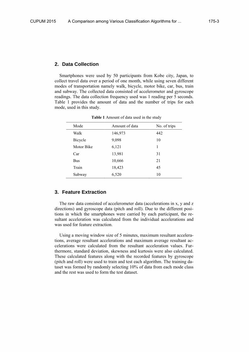
2. Data Collection

Smartphones were used by 50 participants from Kobe city, Japan, to

collect travel data over a period of one month, while using seven different

modes of transportation namely walk, bicycle, motor bike, car, bus, train

and subway. The collected data consisted of accelerometer and gyroscope

readings. The data collection frequency used was 1 reading per 5 seconds.

Table 1 provides the amount of data and the number of trips for each

mode, used in this study.

Table 1 Amount of data used in the study

Mode Amount of data No. of trips

Walk 146,973 442

Bicycle 9,098 10

Motor Bike 6,121 1

Car 13,981 31

Bus 10,666 21

Train 18,423 45

Subway 6,520 10

3. Feature Extraction

The raw data consisted of accelerometer data (accelerations in x, y and z

directions) and gyroscope data (pitch and roll). Due to the different posi-

tions in which the smartphones were carried by each participant, the re-

sultant acceleration was calculated from the individual accelerations and

was used for feature extraction.

Using a moving window size of 5 minutes, maximum resultant accelera-

tions, average resultant accelerations and maximum average resultant ac-

celerations were calculated from the resultant acceleration values. Fur-

thermore, standard deviation, skewness and kurtosis were also calculated.

These calculated features along with the recorded features by gyroscope

(pitch and roll) were used to train and test each algorithm. The training da-

taset was formed by randomly selecting 10% of data from each mode class

and the rest was used to form the test dataset.

CUPUM 2015 A Comparison among Various Classification Algorithms for ... 175-3

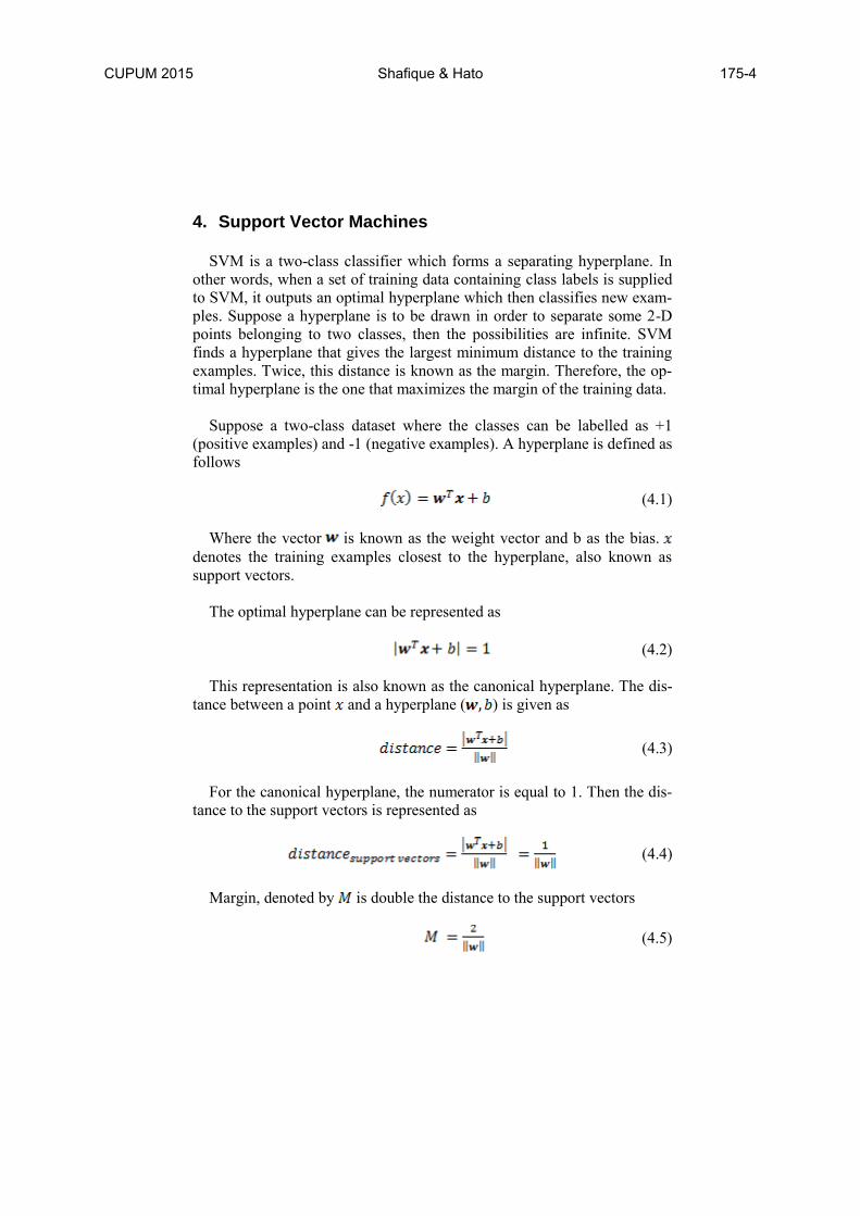
4. Support Vector Machines

SVM is a two-class classifier which forms a separating hyperplane. In

other words, when a set of training data containing class labels is supplied

to SVM, it outputs an optimal hyperplane which then classifies new exam-

ples. Suppose a hyperplane is to be drawn in order to separate some 2-D

points belonging to two classes, then the possibilities are infinite. SVM

finds a hyperplane that gives the largest minimum distance to the training

examples. Twice, this distance is known as the margin. Therefore, the op-

timal hyperplane is the one that maximizes the margin of the training data.

Suppose a two-class dataset where the classes can be labelled as +1

(positive examples) and -1 (negative examples). A hyperplane is defined as

follows

(4.1)

Where the vector is known as the weight vector and b as the bias.

denotes the training examples closest to the hyperplane, also known as

support vectors.

The optimal hyperplane can be represented as

(4.2)

This representation is also known as the canonical hyperplane. The dis-

tance between a point and a hyperplane ( ) is given as

(4.3)

For the canonical hyperplane, the numerator is equal to 1. Then the dis-

tance to the support vectors is represented as

(4.4)

Margin, denoted by is double the distance to the support vectors

(4.5)


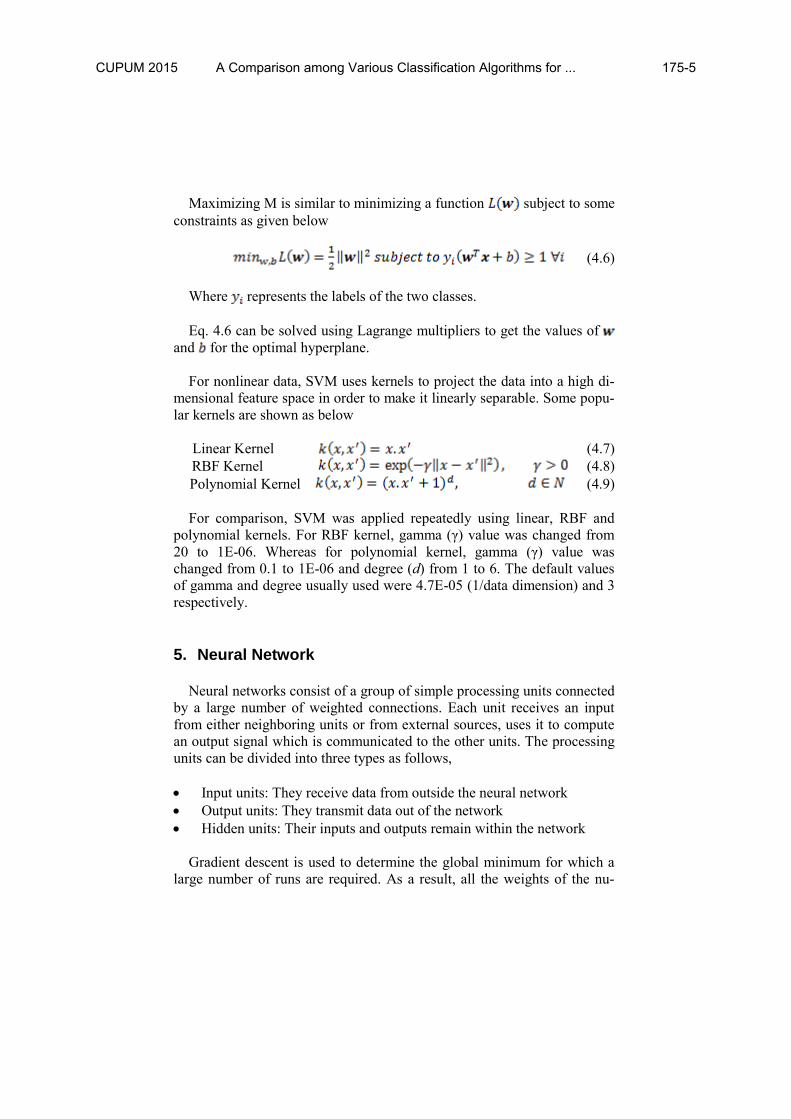
Maximizing M is similar to minimizing a function subject to some

constraints as given below

(4.6)

Where represents the labels of the two classes.

Eq. 4.6 can be solved using Lagrange multipliers to get the values of

and for the optimal hyperplane.

For nonlinear data, SVM uses kernels to project the data into a high di-

mensional feature space in order to make it linearly separable. Some popu-

lar kernels are shown as below

Linear Kernel (4.7)

RBF Kernel (4.8)

Polynomial Kernel (4.9)

For comparison, SVM was applied repeatedly using linear, RBF and

polynomial kernels. For RBF kernel, gamma (γ) value was changed from

20 to 1E-06. Whereas for polynomial kernel, gamma (γ) value was

changed from 0.1 to 1E-06 and degree (d) from 1 to 6. The default values

of gamma and degree usually used were 4.7E-05 (1/data dimension) and 3

respectively.

5. Neural Network

Neural networks consist of a group of simple processing units connected

by a large number of weighted connections. Each unit receives an input

from either neighboring units or from external sources, uses it to compute

an output signal which is communicated to the other units. The processing

units can be divided into three types as follows,

Input units: They receive data from outside the neural network

Output units: They transmit data out of the network

Hidden units: Their inputs and outputs remain within the network

Gradient descent is used to determine the global minimum for which a

large number of runs are required. As a result, all the weights of the nu-


merous connections are continuously modified and hence a final network

is attained after training. This trained network is then used to test the new

data, during which no backpropagation occurs as the weights are already

set during training.

For neural networks, the number of units in the hidden layer or size was

varied from 30 to 50 and maximum number of iterations (default 100)

ranged from 100 to 500.

6. Decision Trees

Decision trees repeatedly split the dataset in order to arrive at a final

outcome. The split is made into branch-like segments and these segments

progressively form an inverted tree, which originates from the starting

node called the root. The root is the only node in the tree which does not

have an incoming segment. The tree terminates at the decision nodes, also

known as leaves or terminals. The decision nodes do not have any out-

going segment and so provide with the final decision from the decision

tree. All the other nodes present within the tree are called internals or test

nodes.

The variables or features associated with the data are used to make each

split. At each node, the variables are tested to determine the most suitable

variable to make the split. This testing is repeated on reaching the next

node and progressively forms a tree. Each terminal node corresponds to a

target class. The accuracy of decision trees can be further improved by us-

ing a method known as boosting.

In case of simple decision trees, minimum number of observations for

the split to take place was reduced from 20 (default) to 2. The complexity

parameter (cp) was varied from 0.1 to 1E-05. In case of boosted decision

trees, SAMME was applied with the complexity parameter ranging from

1E-02 to 1E-05.

7. Random Forest

Random Forest is an ensemble of decision trees. Suppose n number of

trees are grown. Each tree is generated by randomly selecting nearly 63%

of the given training data. The sample data is therefore different for each


tree. The remaining 37% data, known as out of bag (OOB) data, is used to

estimate the error rate. The trees are fully grown without any requirement

of pruning, which is one of the advantages of random forest. At each node

a subset of variables or features is selected and the most suitable feature

among them is used for the split. The size of subset is a variable which is

generally taken as where k is the total number of features. Once the

forest is grown by using the labelled training dataset, the test data is intro-

duced for the prediction. The individual predictions by the trees are aggre-

gated to conclude the final prediction result (i.e. majority vote for classifi-

cation and average for regression).

Sampling was done with and without replacement, while the number of

trees in the forest was varied from 100 to 200.

8. Naïve Bayes

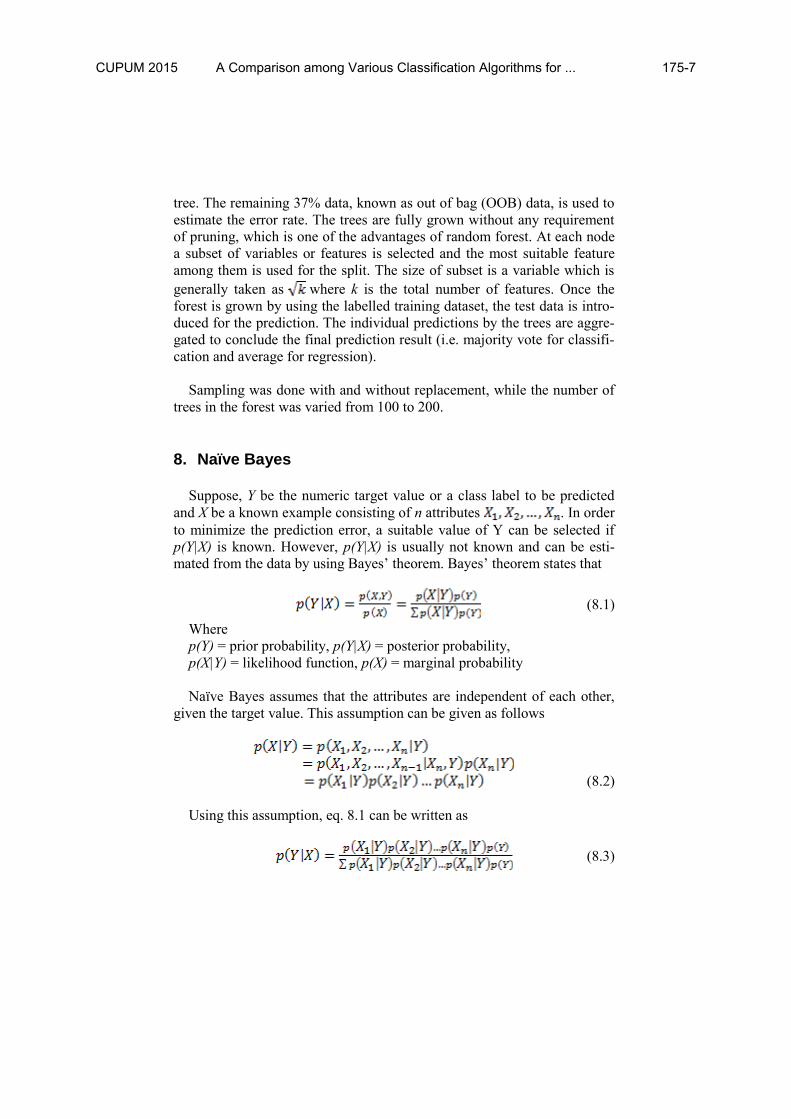
Suppose, Y be the numeric target value or a class label to be predicted

and X be a known example consisting of n attributes . In order

to minimize the prediction error, a suitable value of Y can be selected if

p(Y|X) is known. However, p(Y|X) is usually not known and can be esti-

mated from the data by using Bayes’ theorem. Bayes’ theorem states that

(8.1)

Where

p(Y) = prior probability, p(Y|X) = posterior probability,

p(X|Y) = likelihood function, p(X) = marginal probability

Naïve Bayes assumes that the attributes are independent of each other,

given the target value. This assumption can be given as follows

(8.2)

Using this assumption, eq. 8.1 can be written as

(8.3)


Eq. 8.3 is the fundamental equation of Naïve Bayes classifier. The as-

sumption introduced by Naïve Bayes drastically reduces the number of pa-

rameters to be estimated.

9. Results and Discussion

Each algorithm was tested by manually varying the variables involved,

rather than automatically tuning the algorithm to identify the most suitable

values, because the aim was to observe the computational time for each

change so as to gain an indicator (time) for the comparison of algorithms.

All the calculations were performed on an Intel core i7 3.50 GHz with 32

GB RAM.

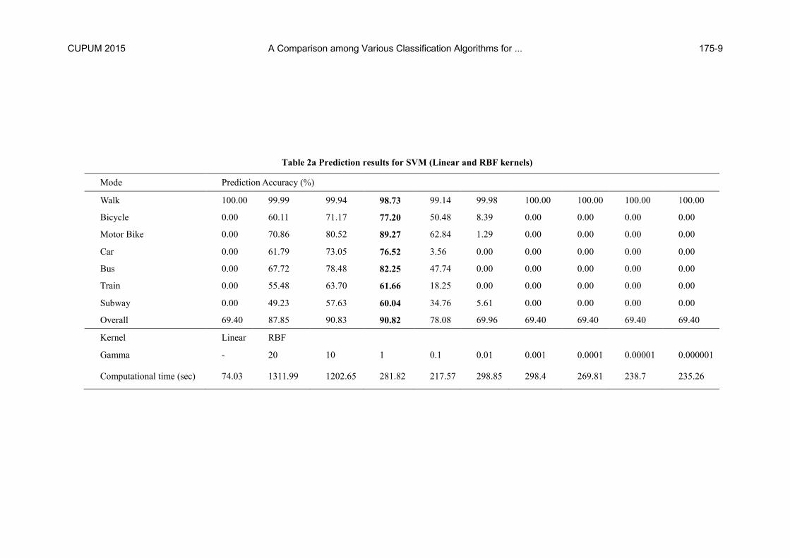
In case of SVM, the prediction accuracies (ratio of data of a certain class

correctly labelled by algorithm to entire data of that certain class) for linear

kernel and RBF kernel (with varying gamma values) are shown in table 2a,

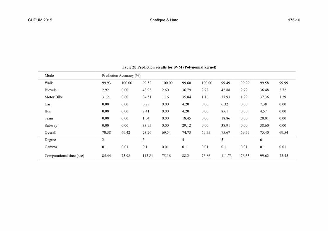
whereas the results for polynomial kernel are given in table 2b. All results

for polynomial kernel are not shown in table 2b because those variable

values were skipped for which the entire data was labelled as walk. The re-

sults propose that both linear and polynomial kernels are not suitable for

smartphone data. Using RBF kernel, the overall accuracy is maximum

when gamma has a value of 10, but a gamma value of 1 gives equally good

results with much less computational time. Furthermore, close inspection

of the results suggest that gamma = 1 is actually yielding better results

mode-wise. Because the amount of data for walk is more that 50% the en-

tire data, therefore a slight increase in its prediction accuracy (in case of

gamma = 10) made it look like a better option.

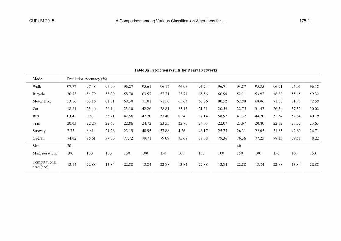
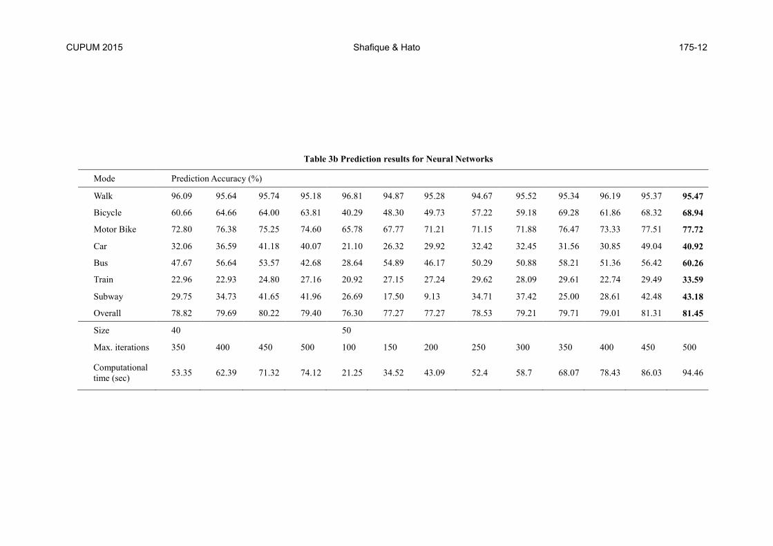
The results for neural networks are shown in tables 3a and 3b. The over-

all prediction accuracy improves as the number of weights is increased by

increasing the size and maximum iterations. The maximum accuracy is

achieved for size 50 and iterations 500, above which the algorithm is una-

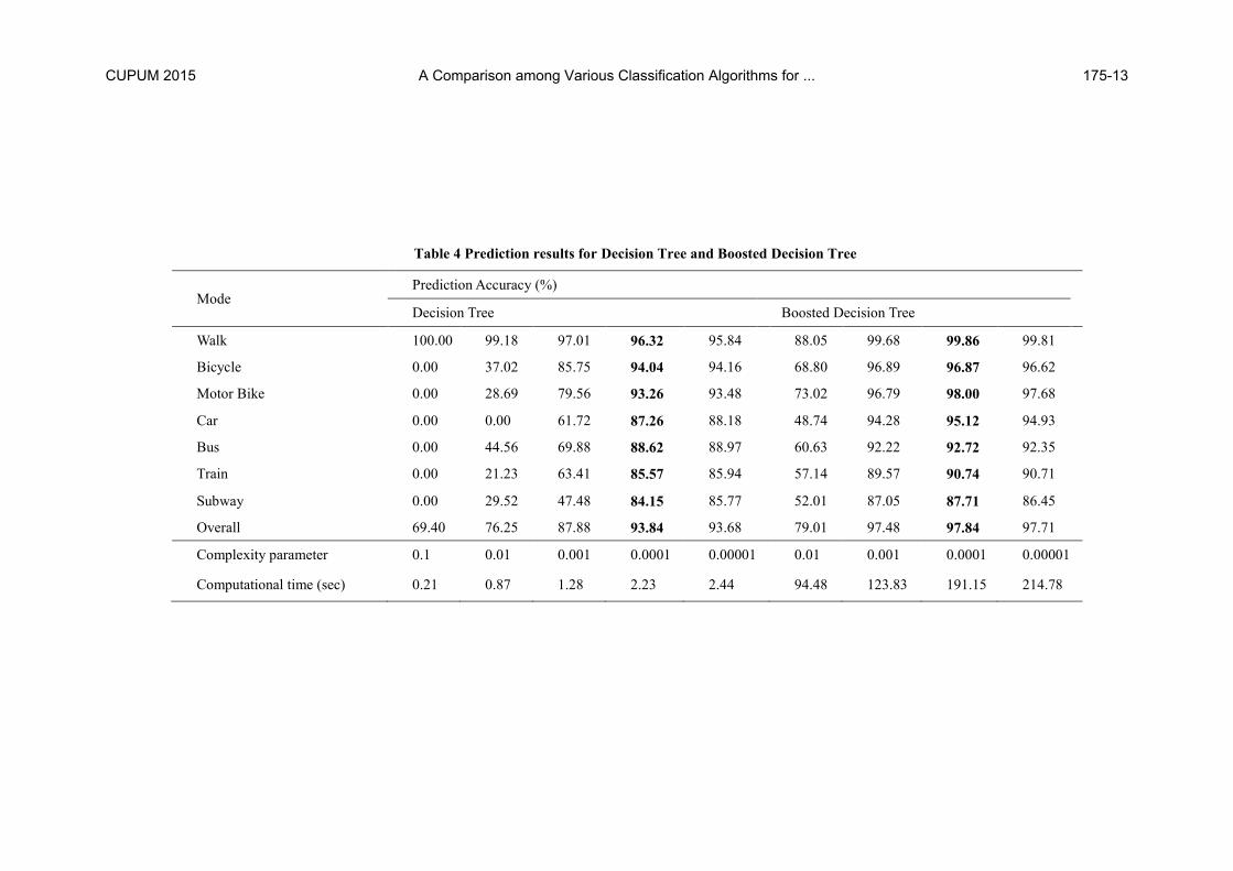
ble to perform due to too many weights. The complexity parameter in de-

cision trees determines the pruning of the tree. The results shown in table 4

demonstrate that the maximum overall accuracy of the decision trees can

be achieved for cp value of 0.0001. But if the decision trees are boosted,

then the prediction accuracy jumps up by around 4% (Table 4). In case of

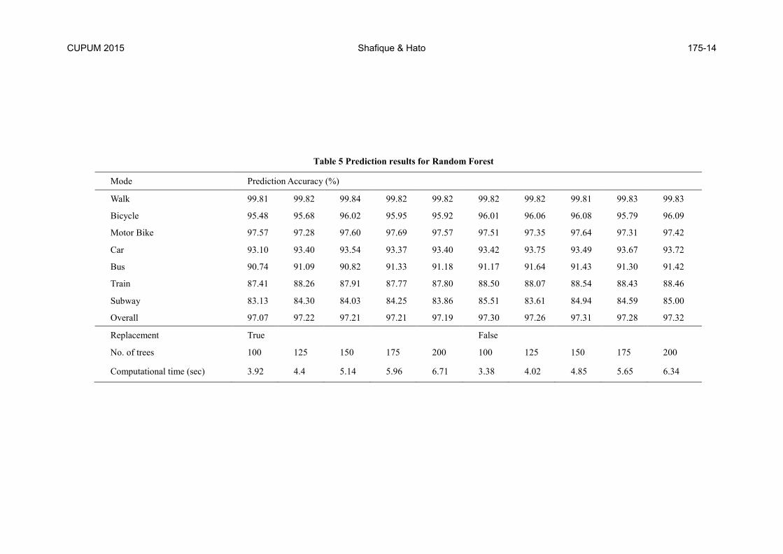
random forest, sampling without replacement provides slightly better re-

sults than with replacement (Table 5).


Table 2a Prediction results for SVM (Linear and RBF kernels)

Mode Prediction Accuracy (%)

Walk 100.00 99.99 99.94 98.73 99.14 99.98 100.00 100.00 100.00 100.00

Bicycle 0.00 60.11 71.17 77.20 50.48 8.39 0.00 0.00 0.00 0.00

Motor Bike 0.00 70.86 80.52 89.27 62.84 1.29 0.00 0.00 0.00 0.00

Car 0.00 61.79 73.05 76.52 3.56 0.00 0.00 0.00 0.00 0.00

Bus 0.00 67.72 78.48 82.25 47.74 0.00 0.00 0.00 0.00 0.00

Train 0.00 55.48 63.70 61.66 18.25 0.00 0.00 0.00 0.00 0.00

Subway 0.00 49.23 57.63 60.04 34.76 5.61 0.00 0.00 0.00 0.00

Overall 69.40 87.85 90.83 90.82 78.08 69.96 69.40 69.40 69.40 69.40

Kernel Linear RBF

Gamma - 20 10 1 0.1 0.01 0.001 0.0001 0.00001 0.000001

Computational time (sec) 74.03 1311.99 1202.65 281.82 217.57 298.85 298.4 269.81 238.7 235.26


Table 2b Prediction results for SVM (Polynomial kernel)


Walk 99.93 100.00 99.52 100.00 99.60 100.00 99.49 99.99 99.58 99.99

Bicycle 2.92 0.00 43.93 2.60 36.79 2.72 42.88 2.72 36.48 2.72

Motor Bike 31.21 0.60 34.51 1.16 35.84 1.16 37.93 1.29 37.36 1.29

Car 0.00 0.00 0.78 0.00 4.20 0.00 6.32 0.00 7.38 0.00

Bus 0.00 0.00 2.41 0.00 4.20 0.00 8.61 0.00 4.57 0.00

Train 0.00 0.00 1.04 0.00 18.45 0.00 18.86 0.00 20.01 0.00

Subway 0.00 0.00 33.95 0.00 29.12 0.00 38.91 0.00 38.60 0.00

Overall 70.38 69.42 73.26 69.54 74.73 69.55 75.67 69.55 75.40 69.54

Degree 2 3 4 5 6

Gamma 0.1 0.01 0.1 0.01 0.1 0.01 0.1 0.01 0.1 0.01



Table 3a Prediction results for Neural Networks


Walk 97.77 97.48 96.00 96.27 95.61 96.17 96.98 95.24 96.71 94.87 95.35 96.01 96.01 96.18

Bicycle 36.53 54.79 55.30 58.70 63.57 57.71 65.71 65.56 66.90 52.31 53.97 48.88 55.45 59.32

Motor Bike 53.16 63.16 61.71 69.30 71.01 71.50 65.63 68.06 80.52 62.98 68.06 71.68 71.90 72.59

Car 18.81 23.46 26.14 23.30 42.26 28.81 23.17 21.51 20.59 22.75 31.47 26.54 37.37 30.02

Bus 0.04 0.67 36.21 42.56 47.20 53.40 0.34 37.14 58.97 41.32 44.20 52.54 52.64 40.19

Train 20.03 22.26 22.67 22.86 24.72 23.55 22.70 24.03 22.07 23.67 20.80 22.52 23.72 23.63

Subway 2.37 8.61 24.76 23.19 40.95 37.88 4.36 46.17 25.75 26.31 22.05 31.65 42.60 24.71

Overall 74.02 75.61 77.06 77.72 79.71 79.09 75.68 77.68 79.36 76.36 77.25 78.13 79.58 78.22

Size 30 40

Max. iterations 100 150 100 150 100 150 100 150 100 150 100 150 100 150

Computational

time (sec) 13.84 22.88 13.84 22.88 13.84 22.88 13.84 22.88 13.84 22.88 13.84 22.88 13.84 22.88


Table 3b Prediction results for Neural Networks


Walk 96.09 95.64 95.74 95.18 96.81 94.87 95.28 94.67 95.52 95.34 96.19 95.37 95.47

Bicycle 60.66 64.66 64.00 63.81 40.29 48.30 49.73 57.22 59.18 69.28 61.86 68.32 68.94

Motor Bike 72.80 76.38 75.25 74.60 65.78 67.77 71.21 71.15 71.88 76.47 73.33 77.51 77.72

Car 32.06 36.59 41.18 40.07 21.10 26.32 29.92 32.42 32.45 31.56 30.85 49.04 40.92

Bus 47.67 56.64 53.57 42.68 28.64 54.89 46.17 50.29 50.88 58.21 51.36 56.42 60.26

Train 22.96 22.93 24.80 27.16 20.92 27.15 27.24 29.62 28.09 29.61 22.74 29.49 33.59

Subway 29.75 34.73 41.65 41.96 26.69 17.50 9.13 34.71 37.42 25.00 28.61 42.48 43.18

Overall 78.82 79.69 80.22 79.40 76.30 77.27 77.27 78.53 79.21 79.71 79.01 81.31 81.45

Size 40 50

Max. iterations 350 400 450 500 100 150 200 250 300 350 400 450 500

Computational

time (sec) 53.35 62.39 71.32 74.12 21.25 34.52 43.09 52.4 58.7 68.07 78.43 86.03 94.46


Table 4 Prediction results for Decision Tree and Boosted Decision Tree


Decision Tree Boosted Decision Tree

Walk 100.00 99.18 97.01 96.32 95.84 88.05 99.68 99.86 99.81

Bicycle 0.00 37.02 85.75 94.04 94.16 68.80 96.89 96.87 96.62

Motor Bike 0.00 28.69 79.56 93.26 93.48 73.02 96.79 98.00 97.68

Car 0.00 0.00 61.72 87.26 88.18 48.74 94.28 95.12 94.93

Bus 0.00 44.56 69.88 88.62 88.97 60.63 92.22 92.72 92.35

Train 0.00 21.23 63.41 85.57 85.94 57.14 89.57 90.74 90.71

Subway 0.00 29.52 47.48 84.15 85.77 52.01 87.05 87.71 86.45

Overall 69.40 76.25 87.88 93.84 93.68 79.01 97.48 97.84 97.71

Complexity parameter 0.1 0.01 0.001 0.0001 0.00001 0.01 0.001 0.0001 0.00001

Computational time (sec) 0.21 0.87 1.28 2.23 2.44 94.48 123.83 191.15 214.78


Table 5 Prediction results for Random Forest


Walk 99.81 99.82 99.84 99.82 99.82 99.82 99.82 99.81 99.83 99.83

Bicycle 95.48 95.68 96.02 95.95 95.92 96.01 96.06 96.08 95.79 96.09

Motor Bike 97.57 97.28 97.60 97.69 97.57 97.51 97.35 97.64 97.31 97.42

Car 93.10 93.40 93.54 93.37 93.40 93.42 93.75 93.49 93.67 93.72

Bus 90.74 91.09 90.82 91.33 91.18 91.17 91.64 91.43 91.30 91.42

Train 87.41 88.26 87.91 87.77 87.80 88.50 88.07 88.54 88.43 88.46

Subway 83.13 84.30 84.03 84.25 83.86 85.51 83.61 84.94 84.59 85.00

Overall 97.07 97.22 97.21 97.21 97.19 97.30 97.26 97.31 97.28 97.32

Replacement True False

No. of trees 100 125 150 175 200 100 125 150 175 200



Moreover, the increase in overall prediction accuracy is minimal with

the increase in the number of trees beyond 100. In order to provide a spe-

cific value for the suitable number of trees, 150 will do as it provides high

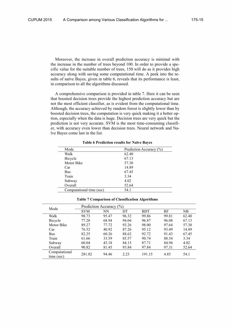
accuracy along with saving some computational time. A peek into the re-

sults of naïve Bayes, given in table 6, reveals that its performance is least,

in comparison to all the algorithms discussed.

A comprehensive comparison is provided in table 7. Here it can be seen

that boosted decision trees provide the highest prediction accuracy but are

not the most efficient classifier, as is evident from the computational time.

Although, the accuracy achieved by random forest is slightly lower than by

boosted decision trees, the computation is very quick making it a better op-

tion, especially when the data is huge. Decision trees are very quick but the

prediction is not very accurate. SVM is the most time-consuming classifi-

er, with accuracy even lower than decision trees. Neural network and Na-

ïve Bayes come last in the list.

Table 6 Prediction results for Naïve Bayes

Mode Prediction Accuracy (%) Walk 62.40

Bicycle 67.13

Motor Bike 57.30

Car 14.89

Bus 67.45

Train 3.34

Subway 4.02

Overall 52.64

Computational time (sec) 54.1

Table 7 Comparison of Classification Algorithms

Mode Prediction Accuracy (%) SVM NN DT BDT RF NB

Walk 98.73 95.47 96.32 99.86 99.81 62.40

Bicycle 77.20 68.94 94.04 96.87 96.08 67.13

Motor Bike 89.27 77.72 93.26 98.00 97.64 57.30

Car 76.52 40.92 87.26 95.12 93.49 14.89

Bus 82.25 60.26 88.62 92.72 91.43 67.45

Train 61.66 33.59 85.57 90.74 88.54 3.34

Subway 60.04 43.18 84.15 87.71 84.94 4.02

Overall 90.82 81.45 93.84 97.84 97.31 52.64

Computational

time (sec) 281.82 94.46 2.23 191.15 4.85 54.1


10. Conclusion and Future Work

This study provides an analysis of the performance of each algorithm by

varying the associated variables and offers a comparison among the algo-

rithms. The results suggest that random forest and boosted decision trees

both provide good prediction accuracies but random forest is relatively

very quick and thus is more suitable for identification of mode of transpor-

tation by employing the sensors’ data collected by smartphones. If the de-

tection is required very quickly, then decision trees can also be used but

the accuracy will fall. This study will assist other researchers in selection

of classification algorithm. Although, the conclusion drawn by this study

holds good for the travel mode detection, for other problems similar study

should be carried out to ascertain the suitable algorithm.

The results discussed in this paper will assist researchers who are striving

to develop methodologies for automatic travel data collection and subse-

quent inference. The successful application of such a methodology will

certainly be a significant improvement in household trip surveys. This will

in turn have a tremendous impact on the formulation of transportation pol-

icies as well as the planning and design of transportation infrastructures.


References

Byon, Y.-J., Abdulhai, B., Shalaby, A.S., 2007. Impact of sampling rate of

GPS-enabled cell phones on mode detection and GIS map matching per-

formance, Transportation Research Board 86th Annual Meeting.

Gonzalez, P., Weinstein, J., Barbeau, S., Labrador, M., Winters, P.,

Georggi, N.L., Perez, R., 2008. Automating mode detection using neural

networks and assisted GPS data collected using GPS-enabled mobile

phones, 15th World congress on intelligent transportation systems.

Moiseeva, A., Timmermans, H., 2010. Imputing relevant information from

multi-day GPS tracers for retail planning and management using data fu-

sion and context-sensitive learning. Journal of Retailing and Consumer

Services 17(3), 189-199.

Pereira, F., Carrion, C., Zhao, F., Cottrill, C.D., Zegras, C., Ben-Akiva,

M., 2013. The Future Mobility Survey: Overview and Preliminary Evalua-

tion, Proceedings of the Eastern Asia Society for Transportation Studies.

Reddy, S., Mun, M., Burke, J., Estrin, D., Hansen, M., Srivastava, M.,

2010. Using mobile phones to determine transportation modes. ACM

Trans. Sen. Netw. 6(2), 1-27.

Shafique, M.A., Hato, E., 2015. Use of acceleration data for transportation

mode prediction. Transportation 42(1), 163-188.

Zhang, L., Dalyot, S., Eggert, D., Sester, M., 2011. Multi-stage approach

to travel-mode segmentation and classification of gps traces, ISPRS Work-

shop on Geospatial Data Infrastructure: from data acquisition and updating

to smarter services.

Zheng, Y., Liu, L., Wang, L., Xie, X., 2008. Learning transportation mode

from raw gps data for geographic applications on the web, Proceedings of

the 17th international conference on World Wide Web. ACM, Beijing,

China, pp. 247-256.


Date post:	09-Mar-2018
Category:	Documents
Upload:	hoangdan
View:	216 times
Download:	1 times

A Comparison among various Classification Algorithms...

Documents