The Effect of Mass Transfer on the Lateral Dynamics of a Uniform Web

Jerry BrownIWEB 2017

Introduction

• This paper starts where I left off with a paper delivered at the last IWEB Conference.

• In it, I attempted to develop a dynamic multi-span model that incorporated shear.

• At the end, I said,• “A YSK-type Timoshenko model has been developed, and it

looks quite plausible. However, it produces a value for the curvature factor that doesn’t make sense. After exhaustive troubleshooting, I’ve concluded that the problem is most likely something of a conceptual nature.”

Introduction

• I was right about that.• And last summer, it finally dawned on me what it was.• The effect of longitudinal strain on the rate of mass flow

from one span to the next has been overlooked.• This phenomenon is fundamental to the analysis of tension,

but we have been missing its role in lateral dynamics.

Introduction (Cont.)

• We all know about the transport of strain equation,

• The subscripts 1 and 2 refer to a span and its downstream companion. V and ε refer to the average velocities and strains in the spans.

2 2

1 1

11

VV

εε

+=

+

Introduction (Cont.)

• It turns out that something similar is behind the acceleration equation - one of the two equations used in lateral dynamics to convert web shape to lateral motion (the other is the normal entry equation).

• I’m going to show you how it can be derived entirely from the same considerations of mass flow used in tension analysis.

First, some terminology

φ has two names – face angle or bending angle,depending on whether we’re talking about the downstream face or an interior cross- section. In both cases, it refers to the change in angle (relative to the y-axis) of a plane that was perpendicular to the beam centerline in its relaxed state.ψ Is the shear angle.

dydx

φ ψ= +

The mass transfer idea

• We’ll start with the simplest beam model, one without shear deformation – the tensioned Euler-Bernoulli (E-B) model.

• The next slide shows what happens when a moment exists at a downstream roller.

• The sequence starts with a web that is running in a steady state between parallel rollers.

Incremental analysis of mass flow

• It’s easy to show how the angle β (boundary defect) depends on strain at the web edge.

• Furthermore, the strain at the edge depends on curvature.

• So,

1/2 /2

dx Vd m o mdt dt W W

εβ= =

2- 2/2

d ym LW dx

ε=

2

2L

o od yd MV V

dt EIdxβ= − = −

Incremental analysis of mass flow (Cont.)

So, now we know,2

2L

od yd V

dt dxβ= −

LL L

dydx

φ β γ= = +

(1)

(2)

Taking the time derivative of (2) and substituting (1).

2

2L L

L od y dd V

dt dtdxγ

φ = − +(3)

This is the mass transfer equation for webs with negligible shear deformation. It leads to the acceleration equation.

Incremental analysis of mass flow (Cont.)

• Here is how it happens.• Since φL = dyL /dx for an E-B beam.

• The cross derivative is eliminated by taking the time derivative of the normal entry equation. The normal entry equation is,

• It defines the lateral velocity of the web on a roller.• The term in parenthesis is called the entry angle. The last term

is the lateral velocity of the roller itself.

dy dzdyL LLVo Ldt dtdxγ = − +

2

2L L L

L ody d y dd d V

dt dt dx dtdxγ

φ = = − +

Incremental analysis of mass flow (Cont.)

• The result is the acceleration equation that Shelton used in his E-B dynamic model.

• Also,

• So, the normal entry equation is,

• Thus, if there is no boundary defect, the web doesn’t move.

2 2 22

2 2 2d y d y d zL L LVodt dx dt

= +

( )dy dzL LVodt dt

β= − +

LL

dydx

γ β− =

Mass flow with shear

Mass flow with shear (Cont.)

• From the Timoshenko beam equations,

• T = tension, A = cross-sectional area, G = shear modulus and n = shear coefficient.

• So, the time derivative of β is,

212

d y nTLM aEI where aAGdx

= = +

2

2d yd LaVodt dx

β= −

Mass flow with shear (Cont.)

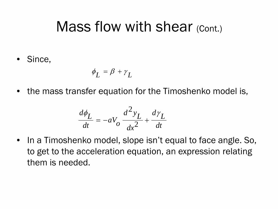
• Since,

• the mass transfer equation for the Timoshenko model is,

• In a Timoshenko model, slope isn’t equal to face angle. So, to get to the acceleration equation, an expression relating them is needed.

L Lφ β γ= +

2

2d d y dL L LaVodt dtdx

φ γ= − +

Acceleration equation (Cont.)

• The necessary equation comes from an analysis of the effect of geometric boundary conditions on beam shape. Details are in the paper. Here is the equation.

• h1, h2 and h3 are constants.• Taking the time derivative and again using the normal entry

equation to eliminate the cross derivative yields,

( ) 01

0 2 3L

L

hy y h hL L

dydx

φ φ= − + +

Acceleration equation (Cont.)

• The acceleration equation for models with shear – short, wide webs.

• When a = 1, then h2 = 1, h1 = h3 = 0, it defaults to the E-B acceleration equation, as it should.

• It passes all three of the validity tests described in the paper.

• When all of the time related terms are zero, it becomes the 4th boundary condition for the Timoshenko steady state model – zero curvature at x = L.

( )2 2 2

12 1132 22 2 2hd y d y d zhdy dd dyL L Lo oL LaV h V h ho o dt L dt dt dt Ldt dx dt

γφ = + − + − − +

The meaning of β

• Since,

• the normal entry equation is,

• Taking the time derivative of this will produce the acceleration equation of the previous slide.

LL L L L

dy anddx

φ ψ φ β γ= − = +

( )dy dzL LVo Ldt dtβ ψ= − − +

The meaning of β (Cont.)

• In other words, the Timoshenko acceleration equation breaks down like this,

( )2 2 2

12 1132 22 2 2hd y d y d zhdy dd dyL L Lo oL LaV h V h ho o dt L dt dt dt Ldt dx dt

γφ = + − + − − +

dd LVo dt dtψβ

= − −

Complementary effect on next span

Effect of roller axis angle on face angle

cos( ) and cos( )1 0 0L Lγ γ θ γ γ θ= = −

φL1 = θ L+ γL1 φ02 = θ0 + γ02

Results for L/W = 1

KL = 0.2, L = 3 inches, T = 46 Lbf, W = 3 inches, h = 0.009 inch, E = 510,000 psi.

Step response to roller shift at downstream end of parallel pair

Side force

Newtons

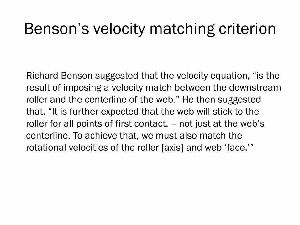
Benson’s velocity matching criterion

Richard Benson suggested that the velocity equation, “is the result of imposing a velocity match between the downstream roller and the centerline of the web.” He then suggested that, “It is further expected that the web will stick to the roller for all points of first contact. – not just at the web’s centerline. To achieve that, we must also match the rotational velocities of the roller [axis] and web ‘face.’”

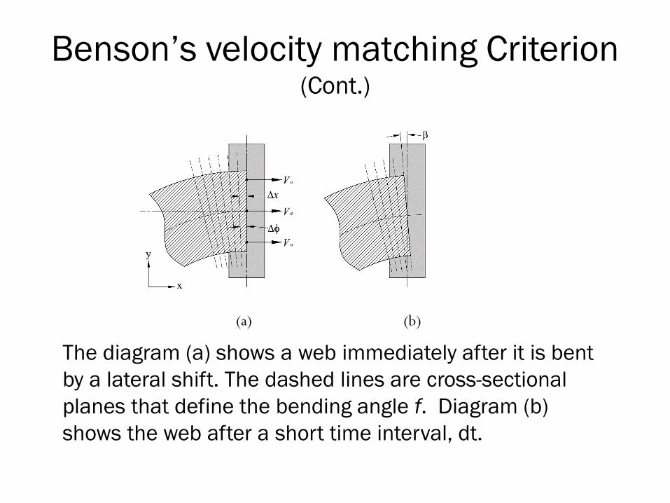
Benson’s velocity matching Criterion (Cont.)

The diagram (a) shows a web immediately after it is bent by a lateral shift. The dashed lines are cross-sectional planes that define the bending angle f. Diagram (b) shows the web after a short time interval, dt.

(a) (b)

Acknowledgements

• Thanks to Sinan Muftu who, after hearing my presentations at the last IWEB conference, drew my attention to Richard Benson’s work.

• Also, thanks to Dilwyn Jones who was kind enough to review and critique this paper as it was being written. He made many helpful suggestions and is the one who discovered that Benson’s acceleration equation is equivalent to the acceleration equation of this paper (even though it looks completely different).