A Compass for Understanding and Using - Census.gov · A Compass for Understanding and Using ......

U.S. Department of CommerceEconomics and Statistics Administration

U.S. CENSUS BUREAU

U S C E N S U S B U R E A UHelping You Make Informed Decisions

A Compass for Understanding and Using

American Community Survey Data

What the Media Need to Know

IssuedNovember 2008

Acknowledgments William H. Frey, Senior Fellow, The Brookings Institution, Brad Edmondson, Consultant, and John P. DeWitt, Senior Associate, Social Science Data Analysis Network, University of Michigan, drafted this handbook for the U.S. Census Bureau’s American Community Survey Offi ce. Kennon R. Copeland and John H. Thompson of National Opinion Research Center at the University of Chicago drafted the technical appendixes. Edward J. Spar, Executive Director, Council of Professional Associations on Federal Statistics, Frederick J. Cavanaugh, Executive Business Director, Sabre Systems, Inc., Susan P. Love, Consultant, Linda A. Jacobsen, Vice President, Domestic Programs, Population Reference Bureau, and Mark Mather, Associate Vice President, Domestic Programs, Population Reference Bureau, provided initial review of this handbook.

Deborah H. Griffi n, Special Assistant to the Chief of the American Community Survey Offi ce, provided the concept and directed the development and release of a series of handbooks entitled A Compass for Understanding and Using American Community Survey Data. Cheryl V. Chambers, Colleen D. Flannery, Cynthia Davis Hollingsworth, Susan L. Hostetter, Pamela D. Klein, Clive R. Richmond, Enid Santana, Anna M. Owens, and Nancy K. Torrieri contributed to the planning and review of this handbook series.

The American Community Survey program is under the direction of Arnold A. Jackson, Associate Director for Decennial Census, Daniel H. Weinberg, Assistant Director for the American Community Survey and Decennial Census, and Susan Schechter, Chief, American Community Survey Offi ce.

Other individuals who contributed to the review and release of these handbooks include Dee Alexander, Herman Alvarado, Mark Asiala, Frank Ambrose, Maryam Asi, Arthur Bakis, Genora Barber, Michael Beaghen, Judy Belton, Lisa Blumerman, Scott Boggess, Ellen Jean Bradley, Stephen Buckner, Whittona Burrell, Edward Castro, Gary Chappell, Michael Cook, Russ Davis, Carrie Dennis, Jason Devine, Joanne Dickinson, Barbara Downs, Maurice Eleby, Sirius Fuller, Dale Garrett, Yvonne Gist, Marjorie Hanson, Greg Harper, William Hazard, Steve Hefter, Douglas Hillmer, Frank Hobbs, Todd Hughes, Trina Jenkins, Nicholas Jones, Anika Juhn, Donald Keathley, Wayne Kei, Karen King, Debra Klein, Vince Kountz, Ashley Landreth, Steve Laue, Van Lawrence, Michelle Lowe, Maria Malagon, Hector Maldonado, Ken Meyer, Louisa Miller, Stanley Moore, Alfredo Navarro, Timothy Olson, Dorothy Paugh, Marie Pees, Marc Perry, Greg Pewett, Roberto Ramirez, Dameka Reese, Katherine Reeves, Lil Paul Reyes, Patrick Rottas, Merarys Rios, J. Gregory Robinson, Anne Ross, Marilyn Sanders, Nicole Scanniello, David Sheppard, Joanna Stancil, Michael Starsinic, Lynette Swopes, Anthony Tersine, Carrie Werner, Edward Welniak, Andre Williams, Steven Wilson, Kai Wu, and Matthew Zimolzak.

Linda Chen and Amanda Perry of the Administrative and Customer Services Division, Francis Grailand Hall, Chief, provided publications management, graphics design and composition, and editorial review for the print and electronic media. Claudette E. Bennett, Assistant Division Chief, and Wanda Cevis, Chief, Publications Services Branch, provided general direction and production management.

A Compass for Understanding and Using American Community Survey Data Issued November 2008

U.S. Department of CommerceCarlos M. Gutierrez,

Secretary

John J. Sullivan, Deputy Secretary

Economics and Statistics AdministrationCynthia A. Glassman,

Under Secretary for Economic Aff airs

U.S. CENSUS BUREAUSteve H. Murdock,

Director

What the Media Need to Know

Suggested Citation

U.S. Census Bureau, A Compass for Understanding

and Using American Community Survey Data:

What the Media Need to KnowU.S. Government Printing Offi ce,

Washington, DC, 2008.

Economics and Statistics Administration

Cynthia A. Glassman,Under Secretary for Economic Aff airs

U.S. CENSUS BUREAU

Steve H. Murdock,Director

Thomas L. Mesenbourg,Deputy Director and Chief Operating Offi cer

Arnold A. JacksonAssociate Director for Decennial Census

Daniel H. WeinbergAssistant Director for ACS and Decennial Census

Susan SchechterChief, American Community Survey Offi ce

ECONOMICS

AND STATISTICS

ADMINISTRATION

What the Media Need to Know iiiU.S. Census Bureau, A Compass for Understanding and Using American Community Survey Data

Contents Foreword...................................................................................................... iv

Introduction ..................................................................................................1

What Is the American Community Survey? ...................................................1

Get New Answers ..........................................................................................2

Topics Covered by the ACS ...........................................................................4

Population and Housing Universes ..............................................................5

ACS Geography .............................................................................................7

Coping With Period Estimates and Sampling Error ..................................... 10

Period Estimates .................................................................................................10Sampling Error ...................................................................................................11

Accessing ACS Data .................................................................................... 12

Aggregate Products ............................................................................................12Public Use Microdata Sample (PUMS) ..................................................................13

FTP: The First Look ..................................................................................... 14

Alternatives to the ACS ............................................................................... 15

Best Use #1: Rankings ................................................................................ 16

Best Use #2: PUMS ...................................................................................... 17

Best Use #3: Mixing It Up ............................................................................ 18

Resources ................................................................................................... 18

Glossary...................................................................................................... 19

Appendixes ................................................................................................A-1

Appendix 1. Understanding and Using Single-Year and Multiyear Estimates .......A-1

Appendix 2. Diff erences Between ACS and Decennial Census Sample Data ........A-8

Appendix 3. Measures of Sampling Error ..........................................................A-11

Appendix 4. Making Comparisons ...................................................................A-18

Appendix 5. Using Dollar-Denominated Data ...................................................A-22

Appendix 6. Measures of Nonsampling Error ...................................................A-24

Appendix 7. Implications of Population Controls on ACS Estimates ..................A-26

Appendix 8. Other ACS Resources ...................................................................A-27

U.S. Census Bureau, A Compass for Understanding and Using American Community Survey Data

iv What the Media Need to Know

Foreword The American Community Survey (ACS) is a nationwide survey designed to provide communities with reliable and timely demographic, social, economic, and housing data every year. The U.S. Census Bureau will release data from the ACS in the form of both single-year and multiyear estimates. These estimates represent concepts that are fundamentally diff erent from those associated with sample data from the decennial census long form. In recognition of the need to provide guidance on these new concepts and the challenges they bring to users of ACS data, the Census Bureau has developed a set of educational handbooks as part of The ACS Compass Products.

We recognize that users of ACS data have varied backgrounds, educations, and experiences. They need diff erent kinds of explanations and guidance to understand ACS data products. To address this diversity, the Census Bureau worked closely with a group of experts to develop a series of handbooks, each of which is designed to instruct and provide guidance to a particular audience. The audiences that we chose are not expected to cover every type of data user, but they cover major stakeholder groups familiar to the Census Bureau.

General data users Congress

High school teachers Puerto Rico Community Survey data users (in Spanish)

Business community Public Use Microdata Sample (PUMS) data users

Researchers Users of data for rural areas

Federal agencies State and local governments

Media Users of data for American Indians and Alaska Natives

The handbooks diff er intentionally from each other in language and style. Some information, including a set of technical appendixes, is common to all of them. However, there are notable diff erences from one handbook to the next in the style of the presentation, as well as in some of the topics that are included. We hope that these diff erences allow each handbook to speak more directly to its target audience. The Census Bureau developed additional ACS Compass Products materials to complement these handbooks. These materials, like the handbooks, are posted on the Census Bureau’s ACS Web site: <www.census.gov/acs/www>.

These handbooks are not expected to cover all aspects of the ACS or to provide direction on every issue. They do represent a starting point for an educational process in which we hope you will participate. We encourage you to review these handbooks and to suggest ways that they can be improved. The Census Bureau is committed to updating these handbooks to address emerging user interests as well as concerns and questions that will arise.

A compass can be an important tool for fi nding one’s way. We hope The ACS Compass Products give direction and guidance to you in using ACS data and that you, in turn, will serve as a scout or pathfi nder in leading others to share what you have learned.

What the Media Need to Know 1U.S. Census Bureau, A Compass for Understanding and Using American Community Survey Data

chosen to represent an area’s population and housing. Based on interviews with this small sample, the Census Bureau uses statistical methods to produce estimates of the characteristics covered by the sur-vey for a broad set of geographic areas such as the nation, all states, congressional districts, counties, and more. “It isn’t the census, so it isn’t a headcount,” says Kenneth Johnson, senior demographer at the Carsey Institute at the University of New Hampshire. “It will do a good job of telling you what percentage of Chicago’s population is Hispanic or poor, but it cannot tell you exactly how many Hispanics or poor people there are in Chicago.”

Reporters need to keep a few rules in mind in order to use the ACS properly, and those who are already using it say the results are well worth the eff ort. “I love the ACS and use it all the time,” says Paula Lavigne, for-merly of the Dallas Morning News. “What we like about the ACS is that you can stand back and see how things are changing,” says Terry Schwadron of The New York Times. “If you have a question about America’s demo-graphics, the answer is likely to be in there some-where,” says Paul Overberg of USA Today.

This guide shows how reporters have used the ACS to write great stories. Most of the time, reporters use this source to grab a statistic on a deadline that helps them make a specifi c point. But the best uses happen off deadline, when you think about the topics you’re cov-ering and then sift through the ACS data to see what it can tell you about those topics. This approach gave Betsy Hammond of the Portland Oregonian a great story about how people in Oregon are less and less likely to be married. And it allowed Paula Lavigne to write an award-winning investigation of high levels of consumer debt in the affl uent suburbs of Dallas, which was published a year before the subprime mortgage market collapsed.

Introduction

Finding fresh data for news stories used to be diffi -cult. Now data are available on a wide range of topics whenever you want it. Rather than having to wait for the once-a-decade census, the U.S. Census Bureau’s American Community Survey (ACS) has emerged as a resource that can strengthen many kinds of news cov-erage and feature stories with annual social, housing, and economic data.

The ACS gives reporters three signifi cant improve-ments in access to demographic information. First, the Census Bureau’s estimates of characteristics for local areas are now updated every year. Second, much of the survey is available through the Census Bureau’s user-friendly Internet site, the American FactFinder. Third, the ACS can sharpen your overall understanding of what is going on in the towns you cover, especially when you learn how to combine it with other sources of demographic information.

The purpose of this guide is to teach reporters how to use this new tool. The guide begins by describing how the ACS is put together and outlining the key concepts you need to know to get the most out of it. It explains the various ways you can fi nd and access ACS data and the best ways for novice and experienced users to use the estimates. There are also brief descriptions of other sources for local area data, as well as step-by-step stories of how journalists have used the ACS to fi nd and improve their published work. A glossary provides defi nitions for key concepts, and a series of appendixes off ers more specifi c information on techni-cal topics, such as interpreting margins of error.

The ACS asks questions of a relatively small num-ber of people living in both housing units (including apartments, single-family homes, mobile homes) and group quarters (including prisons, nursing homes, col-lege dormitories). These people have been randomly

What Is the American Community Survey?

The collection of detailed data about the nation’s popu-lation and housing has been a part of the decennial census since the fi rst census in 1790. Diff erent sam-ples and methods have been used to collect this impor-tant information. In Census 2000, a survey of about one-sixth of the U.S. population and their housing was taken as a snapshot of the nation on Census Day, April 1. It was the nation’s primary source for informa-tion on the socioeconomic characteristics of every

neighborhood in the United States, and it delivered numbers on everything from median income and com-muting to ancestry, educational attainment, and the presence of indoor plumbing. It estimated important local characteristics, but it only happened once every 10 years and was far from perfect. After administering the long form in 1990, the Census Bureau decided it was time for a change.

2 What the Media Need to KnowU.S. Census Bureau, A Compass for Understanding and Using American Community Survey Data

The 2010 Census will not have a long form. The reason for the transition can be summarized in the excerpt below from A Compass for Understanding and Using American Community Survey Data: What Congress Needs to Know.

“After the 1990 census, Congress raised concerns about falling census response rates and rising costs. Congress also expressed an interest in having more timely long-form sample data for policy purposes, not-ing that decennial census long-form data were out of date not long after their release and became less use-ful as the years went by. Congress asked the Census Bureau to explore alternatives to the long form, with the goals of simplifying the census, containing costs, and producing more timely information to inform policy debates and legislative actions.”

The American Community Survey went through a decade of testing and development in a limited number of locations and 4 years of national implementation before it launched nationwide in January 2005 and began surveying monthly samples of about 250,000 housing units. In 2006, a monthly sample of about 20,000 people living in group quarters was added to the housing unit sample.1 Both samples were chosen based on carefully designed methods of selection to provide representation of the entire U.S. population.

After 1 year of continuous data collection, the ACS amasses enough information to release single-year estimates of housing and population characteristics for all areas that have at least 65,000 residents. The 2005 ACS results were released in the summer of 2006, and new 1-year estimates have been released every year since then. After 3 years, the ACS amasses enough data to make estimates for any place with at least 20,000

1 Group quarters include places such as correctional facilities, college dormitories, and nursing homes.

2 For more information on nonsampling errors, see Appendix 6.

residents. The Census Bureau will release the fi rst of these 3-year period estimates in December 2008. The ACS will have collected enough data to release 5-year estimates in 2010 for areas down to the tract and block group level, as the decennial census long form has done in past censuses. All the estimates will be updated for all geographies every year thereafter.

By combining more than 1 year of responses, the ACS is able to provide estimates for smaller geographic areas and increase the precision of its estimates for larger areas because they are based on more inter-views. All sample surveys (including the decennial census long-form sample) have a built-in uncertainty factor known as “sampling error.” This means that each ACS “number” is actually an “estimate” and that the ACS estimates will always be bracketed by margins of error. Understanding and relying on margins of error will allow you to judge how reliable the numbers are. It also means that some estimates of very small popu-lation segments, such as individual neighborhoods, could be based on too few responses to provide use-able estimates in the next few years. The good news is that nonsampling error, a problem that plagued the census long form in the past, has been reduced in the ACS through the use of highly trained interviewers.2

To use the ACS wisely, you need to understand how its design shapes its best uses. Because its products include reliable demographic estimates for most locali-ties in the United States, you can use it to get new answers to basic questions. Because it covers so many diff erent topics, you can use the ACS to anchor inves-tigations of a variety of issues and diff erent groups of people. And because it publishes a new set of esti-mates every year, you can use it to track population trends and explain how communities are changing.

Get New Answers

Paul Overberg of USA Today says that extracting data is only one step in the long process of writing a story about population trends. He says that the process usu-ally begins by asking a general question. “Sometimes I will talk to another reporter for several months before we come up with a question that the data can answer in an interesting way. Once we can do that, we have a story.”

Overberg is an expert in computer-assisted reporting. He has analyzed a huge variety of databases to write front-page stories for USA Today on everything from airline food to baseball salaries, with results that are

imaginative and surprising. Since 1996, Overberg has been having a long conversation with fellow reporter Haya El Nasser about how new immigrants to the United States are assimilating into society. “We’re trying to fi gure out the who and where of it,” he says. “We have known for years about the traditional immigrant gateways—New York, Los Angeles, Miami. But obvi-ously, there’s a lot of moving around once they get into the U.S. We knew they were spreading out, but where were they going? I fi gured that the American Community Survey would have something in it to inform that question.”


Overberg started looking through the ACS tables on migration that are published in the Census Bureau’s online data search engine, the American FactFinder. He eventually downloaded the detailed table on “Resi-dence 1 Year Ago by Citizenship Status in the United States” as an ordinary spreadsheet in the Excel format. Refer to Figure 1 to see the version of this detailed table that is displayed in American FactFinder. This table estimates the number of people who live in the same house they lived in 1 year ago, plus the number who have moved:

• Within the same county.• From a diff erent county in the same state.• From a diff erent state.• From abroad.

Each of these categories is reported for native-born and foreign-born Americans. The foreign born are further reported as either naturalized citizens or not U.S. citizens.

Overberg wanted as much geographic detail as he could get, so he downloaded these 1-year 2006 ACS variables for all U.S. counties that had more than 65,000 residents. Then he used Excel’s delete function to get rid of the variables he did not need. He ended up with a table showing the total number of residents in each county and the number of foreign-born county residents who had moved across county lines in the last year. “I wanted to fi nd the percentage of a place’s total population that was foreign born and had moved there from elsewhere in the U.S. in the previous year,” he says.

The limits of survey-based data required Overberg to make several judgment calls. Some county-level estimates from the ACS are based on a relatively small number of respondents and the smaller the num-ber of responses, the larger the margin of error that surrounds the estimate. Several of the counties that registered large percentages of recent foreign-born

Figure 1. Residence, 1 Year Ago by Citizenship Status in the United States

Source: U.S. Census Bureau, American FactFinder, accessed at <http://factfi nder.census.gov>.


arrivals had margins of error that were large enough to make Overberg and El Nasser question their funda-mental accuracy. So they steered away from counties with relatively small total populations, and they looked at the 2005 ACS to see whether the estimates varied wildly from one year to the next.

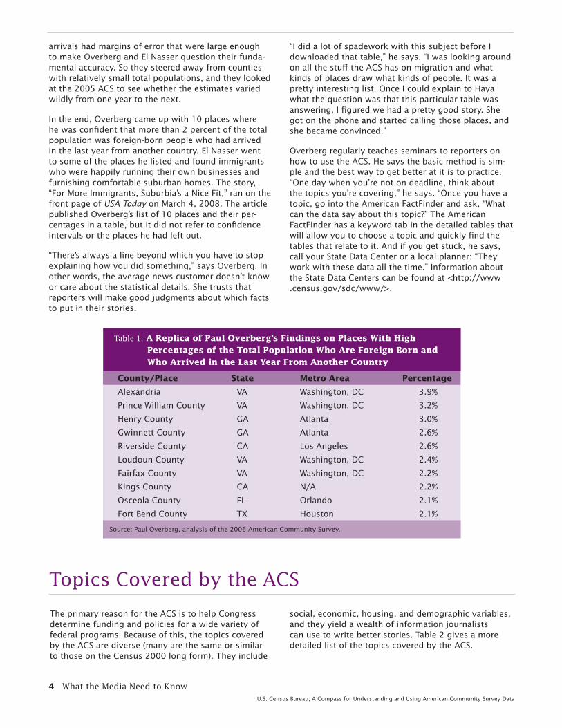
In the end, Overberg came up with 10 places where he was confi dent that more than 2 percent of the total population was foreign-born people who had arrived in the last year from another country. El Nasser went to some of the places he listed and found immigrants who were happily running their own businesses and furnishing comfortable suburban homes. The story, “For More Immigrants, Suburbia’s a Nice Fit,” ran on the front page of USA Today on March 4, 2008. The article published Overberg’s list of 10 places and their per-centages in a table, but it did not refer to confi dence intervals or the places he had left out.

“There’s always a line beyond which you have to stop explaining how you did something,” says Overberg. In other words, the average news customer doesn’t know or care about the statistical details. She trusts that reporters will make good judgments about which facts to put in their stories.

“I did a lot of spadework with this subject before I downloaded that table,” he says. “I was looking around on all the stuff the ACS has on migration and what kinds of places draw what kinds of people. It was a pretty interesting list. Once I could explain to Haya what the question was that this particular table was answering, I fi gured we had a pretty good story. She got on the phone and started calling those places, and she became convinced.”

Overberg regularly teaches seminars to reporters on how to use the ACS. He says the basic method is sim-ple and the best way to get better at it is to practice. “One day when you’re not on deadline, think about the topics you’re covering,” he says. “Once you have a topic, go into the American FactFinder and ask, “What can the data say about this topic?” The American FactFinder has a keyword tab in the detailed tables that will allow you to choose a topic and quickly fi nd the tables that relate to it. And if you get stuck, he says, call your State Data Center or a local planner: “They work with these data all the time.” Information about the State Data Centers can be found at <http://www.census.gov/sdc/www/>.

County/Place State Metro Area Percentage

Alexandria VA Washington, DC 3.9%

Prince William County VA Washington, DC 3.2%

Henry County GA Atlanta 3.0%

Gwinnett County GA Atlanta 2.6%

Riverside County CA Los Angeles 2.6%

Loudoun County VA Washington, DC 2.4%

Fairfax County VA Washington, DC 2.2%

Kings County CA N/A 2.2%

Osceola County FL Orlando 2.1%

Fort Bend County TX Houston 2.1%

Table 1. A Replica of Paul Overberg’s Findings on Places With High Percentages of the Total Population Who Are Foreign Born and Who Arrived in the Last Year From Another Country

Source: Paul Overberg, analysis of the 2006 American Community Survey.

Topics Covered by the ACS

The primary reason for the ACS is to help Congress determine funding and policies for a wide variety of federal programs. Because of this, the topics covered by the ACS are diverse (many are the same or similar to those on the Census 2000 long form). They include

social, economic, housing, and demographic variables, and they yield a wealth of information journalists can use to write better stories. Table 2 gives a more detailed list of the topics covered by the ACS.


Table 2. Subjects Included in the American Community Survey

Demographic CharacteristicsAgeSexHispanic OriginRaceRelationship to Householder

(e.g., spouse)

Economic CharacteristicsIncomeFood Stamps Benefi tLabor Force StatusIndustry, Occupation, and Class

of WorkerPlace of Work and Journey to

WorkWork Status Last YearVehicles AvailableHealth Insurance Coverage*

Social Characteristics Marital Status and Marital History*FertilityGrandparents as CaregiversAncestryPlace of Birth, Citizenship, and

Year of EntryLanguage Spoken at HomeEducational Attainment and

School EnrollmentResidence One Year AgoVeteran Status, Period of Military

Service, and VA Service-Connected Disability Rating*

Disability

Housing CharacteristicsYear Structure BuiltUnits in StructureYear Moved Into UnitRoomsBedroomsKitchen FacilitiesPlumbing FacilitiesHouse Heating FuelTelephone Service AvailableFarm Residence

Financial CharacteristicsTenure (Owner/Renter)Housing ValueRentSelected Monthly Owner Costs

*Marital History, VA Service-Connected Disability Rating, and Health Insurance Coverage are new for 2008. Source: U.S. Census Bureau.

Several ACS questions obtain information for sub-groups of the total U.S. population, such as homeown-ers or people living in family households. The particu-lar subgroup covered by each question is referred to as the “universe.” ACS tables also are based on particular universes. It is important to note which population or housing universe is included in the tabulation when you cite an estimate from the ACS. For example, responses related to marital status are tabulated only if the individual is at least 15 years of age. So in statistics on marriage, the universe is the population 15 years

and over. Similarly, employment characteristics are typically reported only for the population 16 years of age and over.

In the table below, the universe is clearly defi ned as the population 15 years and over. Depending on the data product you are using, the universe may be given either in the individual cells or at the top of the table. Figure 2 shows an example of an ACS detailed table; the universe is circled.

Population and Housing Universes

Geography

Universe:POPULATION 15

YEARS AND OVER: Female

(Estimate)


YEARS AND OVER: Female

(Margin of Error)


YEARS AND OVER: Female; Now married

(Estimate)


YEARS AND OVER: Female; Now married

(Margin of Error)

Alabama 1,924,509 ±3,452 989,309 ±11,521

Alaska 255,676 ±1,636 136,494 ±3,750

Table 3. Example Cells From an ACS Table Showing the Universe and the Margin of Error


Many of these topics contain numerous subtopics. For example, “Journey to Work” includes data on means of transportation (auto, bus, bicycle, walking), travel time (both duration and time departed), and whether

or not a carpool is used. The best way to learn all the details of what is off ered in the ACS is to follow Paul Overberg’s advice—log on and look around.

Knowing about the universe is important to reporting. For example, if you want to calculate the percentage of the population in an area that is married, you’ll need to divide the estimate of the number of married people by the population 15 years and over, not the total popula-tion. It is good practice to publish the fact that an ACS estimate is based on a restricted universe, even if it may seem obvious since, after all, you wouldn’t expect children to get married or hold a job.

Some ACS topics based on restricted population universes include disability, educational attainment, fertility, language, migration, school enrollment, and veteran status. ACS topics based on restricted housing universes include homeownership (tenure), mortgage costs, and vacant units for rent. It is also important to note that the 2005 ACS did not include people living in group quarters, such as jails, college dorms, and

nursing homes. However, the 2006 ACS and subse-quent years did include samples of the group quarters population.

The use of diff erent population and housing universes makes ACS data more meaningful by tailoring each sta-tistic to its relevant group. The Census Bureau always notes the population universe in each table and map, making the universes easy to identify. When deciding how to cite ACS data in a published story, always think about the specifi c universe covered and remember the lack of group quarters data in 2005, which could aff ect comparisons with ACS data from 2006 and later years. The ACS Web site provides valuable guidance about when comparisons are appropriate. Refer to <http://www.census.gov/acs/www/Usedata/compACS.htm>.

Figure 2. Example of a Population Universe




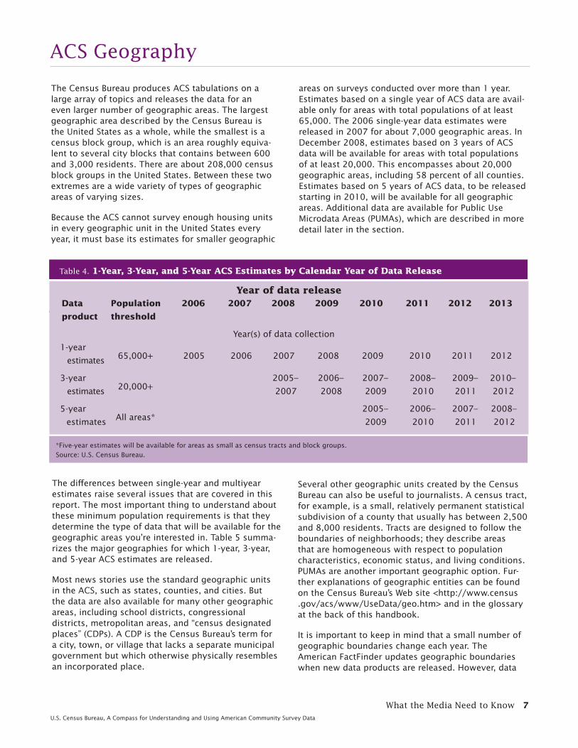
The Census Bureau produces ACS tabulations on a large array of topics and releases the data for an even larger number of geographic areas. The largest geographic area described by the Census Bureau is the United States as a whole, while the smallest is a census block group, which is an area roughly equiva-lent to several city blocks that contains between 600 and 3,000 residents. There are about 208,000 census block groups in the United States. Between these two extremes are a wide variety of types of geographic areas of varying sizes.

Because the ACS cannot survey enough housing units in every geographic unit in the United States every year, it must base its estimates for smaller geographic

areas on surveys conducted over more than 1 year. Estimates based on a single year of ACS data are avail-able only for areas with total populations of at least 65,000. The 2006 single-year data estimates were released in 2007 for about 7,000 geographic areas. In December 2008, estimates based on 3 years of ACS data will be available for areas with total populations of at least 20,000. This encompasses about 20,000 geographic areas, including 58 percent of all counties. Estimates based on 5 years of ACS data, to be released starting in 2010, will be available for all geographic areas. Additional data are available for Public Use Microdata Areas (PUMAs), which are described in more detail later in the section.

ACS Geography

Table 4. 1-Year, 3-Year, and 5-Year ACS Estimates by Calendar Year of Data Release

The diff erences between single-year and multiyear estimates raise several issues that are covered in this report. The most important thing to understand about these minimum population requirements is that they determine the type of data that will be available for the geographic areas you’re interested in. Table 5 summa-rizes the major geographies for which 1-year, 3-year, and 5-year ACS estimates are released.

Most news stories use the standard geographic units in the ACS, such as states, counties, and cities. But the data are also available for many other geographic areas, including school districts, congressional districts, metropolitan areas, and “census designated places” (CDPs). A CDP is the Census Bureau’s term for a city, town, or village that lacks a separate municipal government but which otherwise physically resembles an incorporated place.

Several other geographic units created by the Census Bureau can also be useful to journalists. A census tract, for example, is a small, relatively permanent statistical subdivision of a county that usually has between 2,500 and 8,000 residents. Tracts are designed to follow the boundaries of neighborhoods; they describe areas that are homogeneous with respect to population characteristics, economic status, and living conditions. PUMAs are another important geographic option. Fur-ther explanations of geographic entities can be found on the Census Bureau’s Web site <http://www.census.gov/acs/www/UseData/geo.htm> and in the glossary at the back of this handbook.

It is important to keep in mind that a small number of geographic boundaries change each year. The American FactFinder updates geographic boundaries when new data products are released. However, data

*Five-year estimates will be available for areas as small as census tracts and block groups. Source: U.S. Census Bureau.

Year of data releaseData Population 2006 2007 2008 2009 2010 2011 2012 2013

product threshold

Year(s) of data collection

1-year

estimates 65,000+ 2005 2006 2007 2008 2009 2010 2011 2012

3-year 2005– 2006– 2007– 2008– 2009– 2010–

estimates 20,000+ 2007 2008 2009 2010 2011 2012

5-year 2005– 2006– 2007– 2008–

estimates All areas* 2009 2010 2011 2012


Type of geographic area

Total

number of

areas

Percent of total areas receiving . . .

1-year, 3-year,

& 5-year estimates

3-year & 5-year

estimates only

5-year estimates

only

States and District of Columbia 51 100.0 0.0 0.0

Congressional districts 435 100.0 0.0 0.0

Public Use Microdata Areas* 2,071 99.9 0.1 0.0

Metropolitan statistical areas 363 99.4 0.6 0.0

Micropolitan statistical areas 576 24.3 71.2 4.5

Counties and county equivalents

3,141 25.0 32.8 42.2

Urban areas 3,607 10.4 12.9 76.7

School districts (elementary, secondary, and unifi ed) 14,120 6.6 17.0 76.4

American Indian areas, Alaska Native areas, and Hawaiian homelands 607 2.5 3.5 94.1

Places (cities, towns, and census designated places) 25,081 2.0 6.2 91.8

Townships and villages (minor civil divisions) 21,171 0.9 3.8 95.3

ZIP Code tabulation areas 32,154 0.0 0.0 100.0

Census tracts 65,442 0.0 0.0 100.0

Census block groups 208,801 0.0 0.0 100.0

Table 5. Major Geographic Areas and Type of ACS Estimates Received

* When originally designed, each PUMA contained a population of about 100,000. Over time, some of these PUMAs have gained or lost population. However, due to the population displacement in the greater New Orleans areas caused by Hurricane Katrina in 2005, Louisiana PUMAs 1801, 1802, and 1805 no longer meet the 65,000-population threshold for 1-year estimates. With reference to Public Use Microdata Sample (PUMS) data, records for these PUMAs were combined to ensure ACS PUMS data for Louisiana remain complete and additive.

Source: U.S. Census Bureau, 2008. This tabulation is restricted to geographic areas in the United States. It was based on the population sizes of geographic areas from the July 1, 2007, Census Bureau Population Estimates and geographic boundaries as of January 1, 2007. Because of the potential for changes in population size and geographic boundaries, the actual number of areas receiving 1-year, 3-year, and 5-year estimates may diff er from the numbers in this table.

products released before or just after local bound-ary changes will contain data based on the previous boundaries, an issue that is particularly common with incorporated places and CDPs. It’s important to keep this potential glitch in mind when you’re planning to compare data over several years.

Citing ACS data properly gets more complex as geo-graphic areas get smaller. In 2006, only one-quarter of U.S. counties (783 of 3,141) met or exceeded the popu-lation threshold of 65,000 for single-year estimates. This means that single-year data won’t always be available for the county or counties cited in a particular story. The options for smaller counties are to use the multiyear estimates, to cite statistics for a larger geo-graphic area that includes the county, or to use another source. Demographic data on local areas in the United States are available from sources other than the ACS,

and some of those sources are discussed in the follow-ing sections.

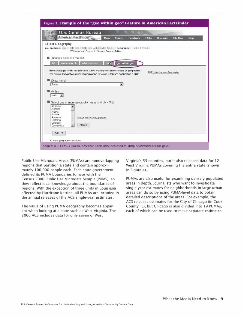
For many reporters, the diverse nature of ACS geography will not be an obstacle because their news organization covers only a single large city or region. Reporters who are writing stories that compare several localities statewide or nationally will need to be a little more careful, but the Census Bureau has created a shortcut that makes large-scale comparisons a lot easier. The American FactFinder interface (described in the “Accessing ACS Data” section), simplifi es the pro-cess by allowing users to select “geo within geo.” When selecting the geography in the detailed tables section of the American FactFinder, click the “geo within geo” tab. You will be directed to identify the subunits (e.g., counties) followed by the main unit of which each sub-unit is a member (e.g., nation or state). Figure 3 shows you an example of this feature.


Public Use Microdata Areas (PUMAs) are nonoverlapping regions that partition a state and contain approxi-mately 100,000 people each. Each state government defi ned its PUMA boundaries for use with the Census 2000 Public Use Microdata Sample (PUMS), so they refl ect local knowledge about the boundaries of regions. With the exception of three units in Louisiana aff ected by Hurricane Katrina, all PUMAs are included in the annual releases of the ACS single-year estimates.

The value of using PUMA geography becomes appar-ent when looking at a state such as West Virginia. The 2006 ACS includes data for only seven of West

Virginia’s 55 counties, but it also released data for 12 West Virginia PUMAs covering the entire state (shown in Figure 4).

PUMAs are also useful for examining densely populated areas in depth. Journalists who want to investigate single-year estimates for neighborhoods in large urban areas can do so by using PUMA-level data to obtain detailed descriptions of the areas. For example, the ACS releases estimates for the City of Chicago (in Cook County, IL), but Chicago is also divided into 19 PUMAs, each of which can be used to make separate estimates.

Figure 3. Example of the “geo within geo” Feature in American FactFinder



Figure 4. PUMAs for West Virginia, 2000


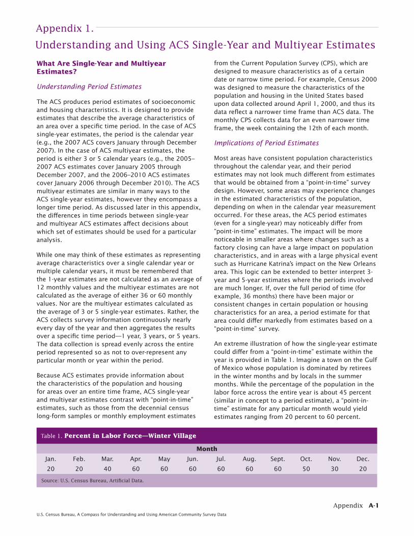
The decennial census is a snapshot of the population taken once every 10 years on Census Day, April 1. But the ACS collects data continuously throughout the year, creating what is known as a period estimate.3 Areas that have a consistent population throughout the year will not see major diff erences between a period esti-mate and the old “snapshot” number. But the estimated numbers may change a lot for areas with populations that fl uctuate considerably between seasons, such as college towns and seasonal retirement areas.4 This is one more reason for using caution when comparing ACS fi gures with those from point-in-time estimates such as Census 2000.

Period Estimates

ACS statistics for small geographic areas also pose spe-cial problems because they are created by pooling sur-vey results collected over 3 or 5 years. “The multiyear estimates are a challenge to everyone who uses the ACS,” says Ken Hodges of Nielsen Claritas. “But they could be especially challenging for journalists, who really can’t devote much space to nuances in the data.” He states that, “A 1-year income estimate for 2006 is clear enough, but a 5-year estimate that covers 2005 through 2009 is a new kind of animal.” Demographers would refer to that as a “5-year period estimate.”

The complications of using multiyear period estimates make single-year estimates easier to describe, but the single-year estimate isn’t always going to be the best choice.5 The trade-off is between accuracy and currency. For many statistics, margins of error for single-year

Coping With Period Estimates and Sampling Error

3 See Appendix 2 for a description of diff erences between the ACS and decennial censuses.4 See Appendix 1 for more information on period estimates. 5 See Appendix 1 for further guidance on use of single-year versus

multiyear estimates.


estimates will be much larger than they are for multi-year estimates. So if accuracy is important, look closely at the multiyear estimate.

In general, trends over time should be examined using nonoverlapping multiyear estimates.6 These are multiyear estimates that are either 3 or 5 years apart, depending on which multiyear estimate was used. For example, to show how a segment of the popula-tion is changing using 3-year estimates, you could use 2005–2007, 2008–2010, and 2011–2013 estimates. The resulting estimates weren’t produced from inter-views in common because they don’t have overlapping years. Unfortunately, this tactic will not be possible for the ACS until the second round of 3-year estimates are available in 2011.

Overlapping multiyear estimates, which will be avail-able beginning in 2009, can still be useful in a more limited way. When you use them in combination with single-year estimates, they can provide insight into areas undergoing rapid change.7 In general though, multiyear estimates should not be used to describe change over a single year. The appendixes at the end of this handbook explain the issues and provide exam-ples of how to use overlapping multiyear estimates.

Sampling Error8

Statistical error is a reality that is diffi cult for report-ers and readers to understand. The decennial census sample had error in its estimates of local areas, but most people used the estimates from the long form as exact numbers describing the population. Error in the census long-form data included nonsampling error, which is diffi cult to measure precisely.9 So the long form’s reputation for great accuracy might not have been deserved in every case, but it endured because statisticians couldn’t tell how inaccurate it was, and the Census Bureau did not provide measures of sam-pling error for these estimates. The good news is that nonsampling error in the ACS is reduced relative to the long form.

All surveys have sampling error. The main diff erence between the census and the ACS is that with the ACS, it’s easy to tell which numbers are good and which aren’t. Margins of error are included with all ACS data products (see Figures 1 and 2) and can be used to assess the quality of the estimates.10 If an estimate is deemed insuffi ciently reliable, then consider using a multiyear estimate instead.

How do you decide when the margin of error for a local estimate is so large that the number should not be used? Paul Overberg compared county-level estimates of foreign-born newcomers for several years to see if they were similar and threw out those that weren’t. Paula Lavigne doesn’t use an estimate if the margin of error is more than 10 percent of the total estimate, and she sometimes throws out other estimates with large margins of error if the local area’s total population is small. Betsy Hammond of the Portland Oregonian says that if the year-to-year change in the characteristic she’s measuring is smaller than the margin of error, she won’t use it.

“What we’re really talking about is what reporters have to do all the time. We use our judgment and only go with things that satisfy a certain comfort level,” says Terry Schwadron, information and technology editor at the New York Times. “The stories should not be about the statistics. They should be about a broader subject, and the numbers should work for the story.”

One of the most common uses of ACS estimates is to make comparisons over time or across geographies. Appendix 4 off ers assistance for these tasks, parti-cularly when comparing ACS data with that of other sources such as the decennial censuses. Appendix 3 also provides guidance on calculating measures of sampling error when aggregating estimates (e.g., com-bining estimates for a three-county area or for fi ve age groups).

6 See Appendix 4 for trend analysis using nonoverlapping estimates.7 See Appendix 1.8 See Appendix 3 for information and methods for calculating measures of sampling error.9 See Appendix 6 for more information on nonsampling error.

10 See Appendix 3 for information on margins of error and confi dence intervals. The Census Bureau provides the margins of error at a 90-percent confi dence level with ACS products. To use other confi -dence levels, see Appendix 3.


The Census Bureau delivers the ACS estimates in stan-dard products that can be categorized as aggregate fi les or microdata (PUMS). Your story’s specifi c focus and subject matter will dictate which of these products is the best fi t.

Aggregate Products

Aggregate products are the most commonly used data products available for the ACS. These include the tables and maps in the American FactFinder <http://factfi nder.census.gov>, which describe the distribu-tions for basic and detailed population and housing queries. These products are referred to as “aggregate” products because the Census Bureau has aggregated the responses from the survey samples into defi ned categories and computed the corresponding estimates, thereby summarizing the data. These products diff er from reports because they off er a variety of options and allow you to work with the data, so you can get the estimate you need. They are most easily found using the American FactFinder, although in a few cases it may be necessary to access them by downloading the whole data set through the Census Bureau’s File Transfer Protocol (FTP) site <www2.census.gov>.

The aggregate products available for ACS data include the following:

• Detailed tables. These are where experienced journalists go fi rst to fi nd the estimates they need. In the American FactFinder, these tables are known as the detailed and custom tables and include the most descriptive and detailed data. These tables feature simple frequency estimates for individual variables and estimates for combinations (such as poverty status by sex and age). Many variables in the detailed tables, such as age, are subdivided into several categories (such as ages 0–17, 18–64, 65 and older, and so on). Detailed tables can also be obtained through FTP.

• Subject tables. These are summarized, topic-specifi c tables based on data from the detailed tables. They are easier to navigate and can be a better choice if you just need a quick overview, or if you’re new to the ACS. Subject tables provide data for some of the most popular topics, such as fi nances, households, and occupational character-istics for a single geography. If your question is simple, subject tables may provide the data you need with a minimum of fuss.

• Ranking tables. These tables compare the 50 states, the District of Columbia, and Puerto Rico according to various characteristics and rank them

from highest to lowest. Ranking tables present state data for nearly 100 diff erent characteristics. These tables can also be viewed as charts, using a link on the page. The charts show the 90-percent confi dence limits around each estimate as an indication of which rankings may be statistically diff erent (meaning that two estimates probably are truly diff erent).

• Geographic comparison tables. These are similar to ranking tables but are available for geo-graphical levels that extend below the state level. Unlike ranking tables, they provide margins of error for the estimates but do not tell you whether or not the diff erences in rankings are statistically signifi cant.

• Data profi les. This product off ers tables that pro-vide summaries of several basic social, economic, housing, and demographic characteristics for each geographic unit. While they are less sophisticated than detailed tables, data profi les do a good job of describing the broad characteristics of a geo-graphic area.

• Narrative profi les. Accessible through data pro-fi les are narrative profi les, which present the data in plain language and use graphics, similar to a news article. These products contain data that are automatically inserted into a preformatted text.

• Selected population profi les. Population profi les are ready-made tabulations for specifi c groups of interest, such as a specifi c ancestry or race. While other ACS profi les provide general information for a geographic area, the selected population profi les use a similar format to provide basic information for a specifi c segment of the population.

• Thematic maps. The maps include two impor-tant features in addition to their categorical color schemes. First, users can quickly identify which other geographic units have a signifi cant statistical diff erence from the selected unit for a particular characteristic. Also, tabular interfaces to the data are readily available as a link on the left of the page.

• Comparison profi les. The comparison profi les show data side-by-side from the 2006 ACS and the 2007 ACS, indicating where there is a statisti-cally signifi cant diff erence between the two sets of estimates. Comparison profi les are only available for 1-year estimates.

Accessing ACS Data


• Summary fi les. The ACS summary fi le includes all detailed tables for all published geographic areas. Summary fi les are accessed from the FTP site.

Public Use Microdata Sample (PUMS)

Accessible through the American FactFinder Web site, microdata fi les are individual response records with all identifying information removed to protect the respondent’s confi dentiality. Aggregate fi les are tables of totals, while microdata fi les are a sample of the indi-vidual survey response records used to arrive at those totals. Microdata fi les are harder to use than the aggre-gate fi les, but have unlimited possibilities because you can create your own tables with the variables of your choosing.

In general, the PUMS fi les are more diffi cult to work with than the aggregate products described above since you have to use a statistical package such as SAS <http://www.sas.com>. Also, the responsibility for producing estimates from PUMS and judging their sta-tistical signifi cance is up to the user. But once you learn how to work with PUMS—the Census Bureau publishes a handbook for PUMS users for those who are inter-ested—the story possibilities are endless. The smallest geographic area on these fi les is the PUMA (see the “ACS Geography” section), which has a minimum popu-lation of 100,000.

PUMS can be used to produce specially tailored tables from the most current ACS. Additionally, many analysts fi nd the PUMS fi les helpful when doing trend analyses to compare PUMS data for each year. An example of using the current PUMS on its own can be found later in “Best Use #2.” The two examples below show how you can compare the current ACS PUMS data with historical decennial census PUMS data.

David Peterson of the Minneapolis Star Tribune used PUMS to fi nd out the facts about a group that is often part of a standard punch line for jokes about Minnesotans. With the help of a research center at the University of Minnesota called IPUMS, Peterson wrote

a query that asked the computer to fi nd the response records of unmarried men of Norwegian ancestry employed as farmers who had been enumerated in the census. The search covered every census from 1930 to 2000, plus the ACS. It revealed that there were tens of thousands of Norwegian bachelor farmers as recently as the 1930s and that half of them were in Minnesota. It also showed that their numbers have been declining steadily since the 1930s and that there weren’t many left in 2005.

The Integrated Public Use Microdata Series or IPUMS <http://usa.ipums.org/usa/> is a 100-person research center that works with social scientists to crunch microdata from a variety of sources, including the ACS. Most of its work is of a far more serious nature. For example, David Knox of the Akron Beacon Journal used IPUMS to look at how the wages of Ohioans have changed at diff erent ages between 1949 and 2006. His series “The Incredible Shrinking Middle Class” was prompted by “agreement on all sides that the middle class in Ohio was in trouble,” he says. After 6 months of work with IPUMS and an analysis of 51 million microdata records, Knox was able to show readers just how bad things were.

“I expected to fi nd that younger workers these days were doing just as well as their parents had done when they were starting out,” he said. “But I found that younger workers in Ohio in 2006 had an aver-age income that was about 25 percent lower than the average income of a young Ohioan in 1970.” Using PUMS, Knox also found that incomes of mid-career workers had gone down dramatically in the last several decades, although the oldest Ohioans were doing com-paratively well.

Knox says that the biggest advantage of using PUMS to look at long-term trends in income is its ability to track how conditions change for diff erent groups. The series began on September 20, 2007, and continued into 2008 with candid interviews with anonymous Ohioans on debt, bankruptcy, and their hopes for their children.


File Transfer Protocol (FTP) is a common way of send-ing large data fi les from one computer to another across the Internet. FTP has several advantages over the familiar protocols used to view Web pages. Many FTP programs, including the latest versions of Internet Explorer, allow users to view fi les on remote computers as if they were on their own machine. You can quickly navigate through several folders and see the contents much faster than you could if you waited for a Web page to load. FTP programs also make it easy to down-load multiple fi les.

The Census Bureau maintains an FTP server, which can be found at <www.census.gov/acs/www/Special/acsftp.html>. But don’t go there until you’ve done some homework. Despite its many benefi ts, getting and using FTP downloads can be challenging.11

It is almost always easier to use the American FactFinder than it is to download ACS data from the FTP site. “The American Community Survey is not par-ticularly friendly to database downloading,” says Overberg. “There is an awful lot of formatting in their raw data that you have to strip out before you can open it in your own database. Just getting a spread-sheet is usually easier.” Since the detailed tables in the American FactFinder contain every variable in the ACS, every variable you can get in the aggregate fi les via FTP is also accessible in the American FactFinder.

There are two cases where an FTP download might be your best option. First, if your story is extremely complex—if it uses multiple data sources including the ACS, and it also uses a lot of ACS data—it might be worthwhile to work with the ACS data so you can include the whole database in your analysis. Most reporters will never need to do this.

Second, FTP is used to provide journalists with embar-goed data when the new year’s ACS data are rolled out. To allow journalists to report on data as soon as they are released, the Census Bureau gives members of the media access to new data sets a few days before their offi cial release. To get access during this “embargo” period, journalists fi ll out a form on a registration page that is available as a link on the Census Bureau’s homepage. Once registered, you’ll be informed of and provided access to data (via FTP) before it is released to the public. This is also the place to register your e-mail so you can get a steady stream of press releases from

the Census Bureau. Stories using embargoed data can-not be published until the release date, but newsrooms might benefi t from downloading ACS data from the FTP site once a year. When the data are in an embargo period, FTP is the only way to get it.

Betsy Hammond, a reporter at the Portland Oregonian, used the FTP site to get brand-new data into a story about statewide trends in marriage. A colleague had been tracking the eff orts of evangelical churches to encourage people to tie the knot. The churches had been running their programs for several years, and the reporters wondered if their eff orts had had any eff ect. What percentage of Oregonians was married, and how did that number compare with 6 years ago?

“I said let’s look at the ACS,” says Hammond. “Maybe it will give this story a peg.” It was August 2007 and Hammond, who subscribes to the Census Bureau’s news service, had noticed that 2006 data from the American Community Survey had come out that week. She went to the American FactFinder and found that the data she needed weren’t posted yet. “I needed the number married in each county in Oregon for diff erent age groups,” she says. “We were being picky, but it was because experts had told us that people are delaying marriage. We needed the age data to see whether this was happening in Oregon. We eventually found that people are marrying later and also that they are less likely to be married in general.”

When she started working with ACS data through the FTP site, Hammond was baffl ed by the way the data were organized. “It was unbelievably hard to under-stand,” she says. “We had to correlate the table num-bers to the data points to see what the statistics were measuring. It was a real chore to fi nd the tables we needed. Then we had to do it again to locate individual counties in Oregon. I had covered the census full-time for a few years, so I knew what I was doing on FTP sites, but this was a real challenge. I showed two diff erent people how I did it and they both laughed at how complicated it was. But once I fi nally was able to extract what we needed, it was beautiful.”

The story, “Marriage Today: Fewer ‘I do’s’ and more just ‘I’s,’” ran on September 23, 2007. It showed that 38 percent of Oregonians ages 20 to 34 were married in 2006, a share about equal to the national average. It also showed that the share of Oregonians who were married had declined sharply between 2000 and 2006 in the 15 Oregon counties and 5 cities for which the ACS published data. In some rural counties the decline over 6 years had been 8 percentage points, which was twice as fast as the 4-point national decline.

FTP: The First Look

11 Paul Overberg suggests that the problems some have experienced may be solved with the release of a new ACS-SF product <http://www.census.gov/acs/www/UseData/sf/tech_doc.htm>.


Comparing Census 2000 with the ACS is not always possible because of diff erences in the way the data are collected. However, Hammond says that the Census Bureau’s tables came with clear instructions on which numbers were comparable and which were not. “They wrote that in plain English and put it in a place where you would defi nitely fi nd it,” she says. Small sample sizes for some counties could also have been a con-cern, but Hammond protected herself by citing per-centages rather than the actual numbers. If the change in the number married between 2000 and 2006 was smaller than the margin of error in the 2006 number, she didn’t use it.

The best way to tackle the ACS as a database is to take a class before you’re on deadline. Several organiza-tions off er training in the use of ACS and other federal databases. Probably the best known is The National Institute for Computer Assisted Reporting (NICAR), which is a joint program of Investigative Reporters and Editors (IRE) and the Missouri School of Journalism. Since 1989, NICAR has trained thousands of journal-ists in the practical skills of fi nding, prying loose, and analyzing all kinds of electronic information. It off ers regular workshops to help reporters navigate the ACS and other federal databases.

Alternatives to the ACS

The Census Bureau runs several surveys and programs besides the ACS that provide high-quality local area data, and your stories may benefi t if you know about these alternative sources. The Census Bureau’s annual Population Estimates Program and the upcoming 2010 Census may each be a better source for informa-tion they have in common with the ACS, specifi cally total population, sex, age, and race/ethnicity for states and counties. For example, the numbers released annually from the Population Estimates Program are the offi cial population totals until the next decennial census. They also indicate the components of popula-tion change (births, deaths, and migration), which are not found elsewhere.

The Current Population Survey (CPS) has collected occupational and economic data monthly since 1947. More recently, an Annual Social and Economic Supplement has been added to the CPS to collect more social information in the survey from about 100,000 households annually. The CPS is often the best source for long-term analyses of economic conditions, because the data are consistent and comparable back to 1947. The CPS does not provide data for counties or metropolitan areas. While it does provide state-level data, they are less statistically reliable than those from the ACS due to a much smaller sample size.

The American Housing Survey (AHS) is a longitudinal survey that collects housing-related data from the same housing units over time. It extends back to the 1970s, collects data at the national level every other year, and for 47 metropolitan areas, about every 6 years. The AHS is ideal for analyzing the change in households and the quality of housing.

Other federal agencies provide related data, some of which may help support your specifi c story better than the ACS can. However, each source has its drawbacks. For example, the Internal Revenue Service releases

estimates of migration between all U.S. counties every year. This is a great resource with lots of potential for journalists, but the only people measured are those who fi le tax returns. So it isn’t a good source if your story is about the migration of low-income groups, for example.

The best demographics reporters use the ACS as one arrow in a quiver full of statistical sources. “What we tell reporters is, you can always get an answer,” says Terry Schwadron. “You have to look at the answer in terms of what the question really is. What we like about the ACS is that you can stand back and see how things are changing. You might not use it to get the numbers on a specifi c neighborhood, but you would use it to get a sense of how things are changing in that neighborhood.”

The New York Times retains Queens College demogra-pher Andrew Beveridge to help reporters use sources well. “We can ask him our questions and get his advice on how those questions might best be answered,” says Schwadron. “He has access to the databases, and he can advise us on the most appropriate data to use to answer the question. We’re looking for guidance to make sure we understand the question in context. We don’t want to just pull numbers out of the air.”

Of course, most of us can’t aff ord to keep a private demographer on call. Professional and academic demographers often are happy to give advice for free. City planning departments, school district planning offi ces, reference librarians, and college sociology departments are all good places to look for advice. Each state maintains an offi cial State Data Center with knowledgeable staff ers to answer your questions. There are also numerous Census Information Centers spread out across the country that can provide valu-able assistance and advice.


Finally, while reporters wait for ACS estimates to become reliable for neighborhoods, small towns, and small rural counties, they should be aware of alterna-tives beyond the federal government. Some private sector companies off er unoffi cial demographic esti-mates at the level of census tracts and ZIP Codes that use statistical models to “age” data from the decennial census and other sources. In many cases, these compa-nies will provide these data on request from reporters for free, in exchange for a credit. However, many such vendors do not have offi cial data and release their data using proprietary models based on assumptions that are not always verifi able.

You should look at databases in the same way that you judge human sources. First, identify the data sets that could be most informative for your topic. Then judge their reliability and also ask yourself if the data are appropriate for the topic of your story. The ACS will often turn out to be the best choice because of its great breadth and fl exibility, but there will be times when you will need a diff erent source to get the job done. If you have questions about which source to use, contact the State Data Center or a professional demographer. They work with the data on a regular basis, so they can point you in the right direction.

Here are a few of the best ways reporters use the ACS, told in their own words.

Best Use #1: Rankings

“The biggest advantage of the ACS is the annual updates,” says Cheryl Russell, who has spent the last 30 years writing about demographic change. “It is incredible that these statistics are fi nally being updated every year. But getting to the statistics is like peeling an onion. It takes a long time to get what you want, and it can be tedious. You need patience.”

Russell, the editor-in-chief of New Strategist Publications and former top editor at American Demo-graphics magazine, writes an e-mail newsletter and blog that specialize in checking conventional wisdom against the facts, see <http://www.newstrategist.com>. A few months ago, she noticed pundits saying that the mortgage crisis was due to Americans using their homes as ATM machines by taking out home equity loans and second mortgages. “The sources they quoted were macroeconomic statistics,” she says. “It is easy to be sold by those kinds of statistics. But with the ACS it’s just as easy to look at the behavior of individual households.”

Russell went to the American FactFinder and found two subject tables that put the home equity story in context. Subject Table #S2503, “Financial Characteris-tics,” gave her the big picture: there were an estimated 75,086,485 owner-occupied housing units in the United States in 2006, give or take a few thousand (remember, the numbers are more accurate as the sample gets larger). Then she went to Subject Table #S2506, “Financial Characteristics for Housing Units With a Mortgage,” and found that an estimated 51,234,170 owner-occupied housing units were car-rying a mortgage. In other words, about one-third of homeowners don’t have any mortgage debt at all.

Going further with Subject Table #S2506, Russell saw that an estimated 25.4 percent of homeowners who had a mortgage also had a second mortgage or a home equity loan, but not both: 19.3 percent had a home

equity loan only, and 6.1 percent had a second mort-gage. Only 1.1 percent had both. Simple multiplication revealed the estimate that 9,888,195 homeowners with a mortgage also had a home equity loan. That is 13.1 percent of all homeowners, hardly universal behavior.

To fi nd out if over-mortgaged America is more of a problem in some places than others, it is easy to use the ACS to fi nd debt hot spots.

• Choose the “Detailed Tables” option within the most recent ACS in the American FactFinder.

• Select the geography you’d like to analyze, such as all metropolitan areas within a state or met-ropolitan and “micropolitan” areas in the United States.

• Using the “subject” tab, fi nd all the detailed tables that match the terms “owner-occupied” and “mort-gage.”

• Detailed Table #B25081, “Mortgage Status – Uni-verse: Owner-Occupied Housing Units,” shows the estimated number of owner-occupied hous-ing units in each area, the estimated number that have any kind of mortgage, the estimated number with second mortgages, and the estimated num-ber with home equity loans.

• Download this table as a spreadsheet fi le. When you open it, you’ll notice that the data are spread out horizontally instead of vertically, a problem you must correct yourself. You’ll also notice that each number is followed by an estimate of its margin of error. The margins of error may seem unnecessary and deleting them will make your table smaller. But, it’s important to study them before you make any conclusions, especially comparisons.


• The resulting table allows you to calculate the percentage of all owner-occupied housing units in various places that have two mortgages, or a mortgage and a home-equity loan, or no mortgage debt at all.

Now you’re cooking with facts. This exercise reveals that in 2006, there were seven metropolitan areas in the United States where about half of all homeowners did not have any kind of mortgage debt at all. Four of them are in Texas (Odessa, Beaumont, McAllen, and Brownsville) two are in West Virginia (Wheeling and Charleston), and the seventh is Johnstown, Pennsylvania. There are also 25 metropolitan areas

where at least one-quarter of homeowners carry a sec-ond mortgage or home equity loan. Eighteen of these are in the West, and of those, fi ve are in Colorado, six are in California. Only two (Washington, DC, and Bridgeport, Conneticut) are in the Northeast. This list is loaded with glamorous towns like Santa Cruz and Boulder, and it is evidence that many people are living high by leveraging themselves to the hilt.

“The ACS is the homework that every reporter needs to do,” says Russell. “You can’t really explain the world unless you are literate about statistics, and the ACS is a great place to learn.”

Best Use #2: PUMS

Sacramento is a hot spot for the home mortgage crisis. Investigations have suggested that one of the reasons for the crisis is that lenders allowed mortgage appli-cants to infl ate their stated incomes far above what they really made. “Behind the Meltdown,” which ran in the Sacramento Bee on Sunday, November 18, 2007, put a local spin on this aspect of the story. Using a variety of sources anchored by the Public Use Micro-data Sample of the ACS, the story detailed large gaps between the incomes listed on 2006 homeowner’s loan applications in the Sacramento area, and the same incomes as estimated by the Census Bureau.

Sacramento Bee reporter Phil Reese used a database from the Federal Home Mortgage Disclosure Act to fi nd the listed incomes of individual loan applicants who originated fi rst lien loans for home purchases in the Sacramento metropolitan area. The query was designed to exclude investors. “With that I had the declared income of everyone who bought a home they planned to use as their residence in 2006,” he says. These data were for individual loan applicants, but they contained ZIP Codes that allowed Reese to aggregate them into median incomes at the county level.

Next, Reese used the ACS to fi nd the median income of owner-occupied households with a mortgage who had moved within the last year (2005–2006). “This num-ber gave me everyone who had used a mortgage to purchase a home in 2006 that they planned to live in,” he says. “There were slight diff erences in how the two

sources measured income, but they were small enough that we felt we could ignore them.”

Reese needed to use a PUMS extract instead of aggre-gate data because the American FactFinder did not allow him to specify owner-occupied households with a mortgage who had moved in the last year. “The slice of the population I needed had one too many conditions,” he says. “But I had used PUMS before with Census 2000, and the ACS PUMS is actually easier to use than the Census 2000 data set. It takes a little getting used to, but there are tons of stories in PUMS.”

Reese learned to use PUMS by going to a NICAR work-shop. “When I fi rst started working with the ACS PUMS, it took an hour or so to fi gure out where things were and to build queries. The site has a specialized query function, and the documentation has to be long, so you have to fi gure out exactly where all the codes should be. But if you are familiar with database management software, it should be no problem.”

The Sacramento Bee’s Web site drove the story home with interactive maps that showed the data and income gaps for each county. “Once I got the two data sources to line up at the county level, the mapping part was easy,” says Reese. In the Sacramento Metropolitan Area, PUMAs lined up with the county boundaries that he needed to present his results. This is not always the case, particularly in some New England states.


There is power in the mix. Paula Lavigne is a reporter for the Dallas Morning News who trained herself in computer-assisted reporting by joining the e-mail list serve of NICAR. “In 2004, I noticed stories about layoff s and foreclosures that were coming out of Collin County, which contains the wealthiest parts of the Dallas metro,” she says. “Social service agencies in Collin County were actually getting requests from people to help pay for their kids’ private schools or their Mercedes-Benz. These were affl uent people, but they were living way beyond their means. The pursuit of stuff had taken on a life of its own.”

Lavigne went to a press offi cer for Claritas and, in exchange for attribution, got the company’s estimates of personal debt for households in diff erent parts of Collin County. She also got the number of personal bankruptcies and foreclosures over the last several years from private and federal sources. “But I wouldn’t have had a story without the ACS,” she says. “I used it to fi nd the counties in the U.S. that had the highest estimated median household incomes, home values, household size, and number of children. Then I com-pared the fi nancial statistics for those counties against the stats for Collin.” For example, Lavigne got the estimated number of owner-occupied housing units in various counties from the ACS, and then compared that number against the number of foreclosures and bank-ruptcies in each county to get a rate.

“I found that Collin County really did stand out among affl uent counties for the share of people who are in economic trouble,” she said. “The ACS helped put the Collin County numbers in context.”

Once she knew there was a story, Lavigne kept using the ACS to assist her reporting. “I looked at where people really diverged in their spending,” she said. “The ACS told me the places that had the highest median household incomes, so I went to those places and looked for signs of foreclosure. I also used the ACS to make a profi le of the typical Collin County family, and then I went out and tried to fi nd people who fell into that description.”

Lavigne’s series, “The Price of Prosperity,” debuted on the front page of the Sunday edition of the Dallas Morning News on August 14, 2005. It drew record numbers of readers and made Lavigne a fi nalist for a 2006 Livingston Award for excellence, given to jour-nalists under the age of 35. A year later, as the magni-tude of the debt and foreclosure story was becoming more evident, Lavigne revisited her sources and ran an update. She found that most Collin residents were even deeper in debt, but focused most of the story on residents who were fi nding a way out.

Best Use #3: Mixing It Up

Resources

Investigative Reporters and Editors (IRE): <http://www.ire.org>

National Institute for Computer-Assisted Reporting, a program of IRE: <http://www.nicar.org>

IPUMS USA: <http://usa.ipums.org>


Glossary

Accuracy. One of four key dimensions of survey quality. Accuracy refers to the diff erence between the survey estimate and the true (unknown) value. Attributes are measured in terms of sources of error (for example, coverage, sampling, nonresponse, measurement, and processing).

American Community Survey Alert. This periodic electronic newsletter informs data users and other interested parties about news, events, data releases, congressional actions, and other developments associated with the ACS. See <http://www.census.gov/acs/www/Special/Alerts/Latest.htm>.

American FactFinder (AFF). An electronic system for access to and dissemination of Census Bureau data on the Internet. AFF off ers prepackaged data products and user-selected data tables and maps from Census 2000, the 1990 Census of Population and Housing, the 1997 and 2002 Economic Censuses, the Population Estimates Program, annual economic surveys, and the ACS.

Block group. A subdivision of a census tract (or, prior to 2000, a block numbering area), a block group is a cluster of blocks having the same fi rst digit of their four-digit identifying number within a census tract.

Census geography. A collective term referring to the types of geographic areas used by the Census Bureau in its data collection and tabulation operations, including their structure, designations, and relationships to one another. See <http://www.census.gov/geo/www/index.html>.

Census tract. A small, relatively permanent statistical subdivision of a county delineated by a local committee of census data users for the purpose of presenting data. Census tract boundaries normally follow visible features, but may follow governmental unit boundaries and other nonvisible features; they always nest within counties. Designed to be relatively homogeneous units with respect to population characteristics, economic status, and living conditions at the time of establishment, census tracts average about 4,000 inhabitants.

Coeffi cient of variation (CV). The ratio of the standard error (square root of the variance) to the value being estimated, usually expressed in terms of a percentage (also known as the relative standard

deviation). The lower the CV, the higher the relative reliability of the estimate.

Comparison profi le. Comparison profi les are available from the American Community Survey for 1-year estimates beginning in 2007. These tables are available for the U.S., the 50 states, the District of Columbia, and geographic areas with a population of more than 65,000.

Confi dence interval. The sample estimate and its standard error permit the construction of a confi dence interval that represents the degree of uncertainty about the estimate. A 90-percent confi dence interval can be interpreted roughly as providing 90 percent certainty that the interval defi ned by the upper and lower bounds contains the true value of the characteristic.

Confi dentiality. The guarantee made by law (Title 13, United States Code) to individuals who provide census information, regarding nondisclosure of that information to others.

Consumer Price Index (CPI). The CPI program of the Bureau of Labor Statistics produces monthly data on changes in the prices paid by urban consumers for a representative basket of goods and services.

Controlled. During the ACS weighting process, the intercensal population and housing estimates are used as survey controls. Weights are adjusted so that ACS estimates conform to these controls.

Current Population Survey (CPS). The CPS is a monthly survey of about 50,000 households conducted by the Census Bureau for the Bureau of Labor Statistics. The CPS is the primary source of information on the labor force characteristics of the U.S. population.

Current residence. The concept used in the ACS to determine who should be considered a resident of a sample address. Everyone who is currently living or staying at a sample address is considered a resident of that address, except people staying there for 2 months or less. People who have established residence at the sample unit and are away for only a short period of time are also considered to be current residents.

Custom tabulations. The Census Bureau off ers a wide variety of general purpose data products from the American Community Survey (ACS). These products are designed to meet the needs of the majority of data


users and contain predefi ned sets of data for standard census geographic areas, including both political and statistical geography. These products are available on the American FactFinder and the ACS Web site.

For users with data needs not met through the general purpose products, the Census Bureau off ers “custom” tabulations on a cost-reimbursable basis, with the American Community Survey Custom Tabulation program. Custom tabulations are created by tabulating data from ACS microdata fi les. They vary in size, complexity, and cost depending on the needs of the sponsoring client.

Data profi les. Detailed tables that provide summaries by social, economic, and housing characteristics. There is a new ACS demographic and housing units profi le that should be used if offi cial estimates from the Population Estimates Program are not available.

Detailed tables. Approximately 1,200 diff erent tables that contain basic distributions of characteristics. These tables provide the most detailed data and are the basis for other ACS products.

Disclosure avoidance (DA). Statistical methods used in the tabulation of data prior to releasing data products to ensure the confi dentiality of responses. See Confi dentiality.

Estimates. Numerical values obtained from a statistical sample and assigned to a population parameter. Data produced from the ACS interviews are collected from samples of housing units. These data are used to produce estimates of the actual fi gures that would have been obtained by interviewing the entire population using the same methodology.

File Transfer Protocol (FTP) site. A Web site that allows data fi les to be downloaded from the Census Bureau Web site.

Five-year estimates. Estimates based on 5 years of ACS data. These estimates refl ect the characteristics of a geographic area over the entire 5-year period and will be published for all geographic areas down to the census block group level.

Geographic comparison tables. More than 80 single-variable tables comparing key indicators for geographies other than states.

Geographic summary level. A geographic summary level specifi es the content and the hierarchical relationships of the geographic elements that are

required to tabulate and summarize data. For example, the county summary level specifi es the state-county hierarchy. Thus, both the state code and the county code are required to uniquely identify a county in the United States or Puerto Rico.

Group quarters (GQ) facilities. A GQ facility is a place where people live or stay that is normally owned or managed by an entity or organization providing housing and/or services for the residents. These services may include custodial or medical care, as well as other types of assistance. Residency is commonly restricted to those receiving these services. People living in GQ facilities are usually not related to each other. The ACS collects data from people living in both housing units and GQ facilities.

Group quarters (GQ) population. The number of persons residing in GQ facilities.

Item allocation rates. Allocation is a method of imputation used when values for missing or inconsistent items cannot be derived from the existing response record. In these cases, the imputation must be based on other techniques such as using answers from other people in the household, other responding housing units, or people believed to have similar characteristics. Such donors are refl ected in a table referred to as an allocation matrix. The rate is the percentage of times this method is used.

Margin of error (MOE). Some ACS products provide an MOE instead of confi dence intervals. An MOE is the diff erence between an estimate and its upper or lower confi dence bounds. Confi dence bounds can be created by adding the margin of error to the estimate (for the upper bound) and subtracting the margin of error from the estimate (for the lower bound). All published ACS margins of error are based on a 90-percent confi dence level.

Multiyear estimates. Three- and fi ve-year estimates based on multiple years of ACS data. Three-year estimates will be published for geographic areas with a population of 20,000 or more. Five-year estimates will be published for all geographic areas down to the census block group level.

Narrative profi le. A data product that includes easy-to-read descriptions for a particular geography.

Nonsampling error. Total survey error can be classifi ed into two categories—sampling error and nonsampling error. Nonsampling error includes measurement errors due to interviewers, respondents, instruments, and mode; nonresponse error; coverage error; and processing error.


Period estimates. An estimate based on information collected over a period of time. For ACS the period is either 1 year, 3 years, or 5 years.

Point-in-time estimates. An estimate based on one point in time. The decennial census long-form estimates for Census 2000 were based on information collected as of April 1, 2000.

Population Estimates Program. Offi cial Census Bureau estimates of the population of the United States, states, metropolitan areas, cities and towns, and counties; also offi cial Census Bureau estimates of housing units (HUs).

Public Use Microdata Area (PUMA). An area that defi nes the extent of territory for which the Census Bureau releases Public Use Microdata Sample (PUMS) records.

Public Use Microdata Sample (PUMS) fi les. Computerized fi les that contain a sample of individual records, with identifying information removed, showing the population and housing characteristics of the units, and people included on those forms.

Puerto Rico Community Survey (PRCS). The counterpart to the ACS that is conducted in Puerto Rico.

Quality measures. Statistics that provide information about the quality of the ACS data. The ACS releases four diff erent quality measures with the annual data release: 1) initial sample size and fi nal interviews; 2) coverage rates; 3) response rates, and; 4) item allocation rates for all collected variables. The ACS Quality Measures Web site provides these statistics each year. In addition, the coverage rates are also available for males and females separately.

Reference period. Time interval to which survey responses refer. For example, many ACS questions refer to the day of the interview; others refer to “the past 12 months” or “last week.”

Residence rules. The series of rules that defi ne who (if anyone) is considered to be a resident of a sample address for purposes of the survey or census.

Sampling error. Errors that occur because only part of the population is directly contacted. With any sample, diff erences are likely to exist between the characteristics of the sampled population and the larger group from which the sample was chosen.

Sampling variability. Variation that occurs by chance because a sample is surveyed rather than the entire population.

Selected population profi les. An ACS data product that provides certain characteristics for a specifi c race or ethnic group (for example, Alaska Natives) or other population subgroup (for example, people aged 60 years and over). This data product is produced directly from the sample microdata (that is, not a derived product).

Single-year estimates. Estimates based on the set of ACS interviews conducted from January through December of a given calendar year. These estimates are published each year for geographic areas with a population of 65,000 or more.

Standard error. The standard error is a measure of the deviation of a sample estimate from the average of all possible samples.

Statistical signifi cance. The determination of whether the diff erence between two estimates is not likely to be from random chance (sampling error) alone. This determination is based on both the estimates themselves and their standard errors. For ACS data, two estimates are “signifi cantly diff erent at the 90 percent level” if their diff erence is large enough to infer that there was a less than 10 percent chance that the diff erence came entirely from random variation.

Subject tables. Data products organized by subject area that present an overview of the information that analysts most often receive requests for from data users.

Summary fi les. Consist of detailed tables of Census 2000 social, economic, and housing characteristics compiled from a sample of approximately 19 million housing units (about 1 in 6 households) that received the Census 2000 long-form questionnaire.

Thematic maps. Display geographic variation in map format from the geographic ranking tables.

Three-year estimates. Estimates based on 3 years of ACS data. These estimates are meant to refl ect the characteristics of a geographic area over the entire 3-year period. These estimates will be published for geographic areas with a population of 20,000 or more.

Appendix A-1U.S. Census Bureau, A Compass for Understanding and Using American Community Survey Data

What Are Single-Year and Multiyear Estimates?

Understanding Period Estimates

The ACS produces period estimates of socioeconomic and housing characteristics. It is designed to provide estimates that describe the average characteristics of an area over a specifi c time period. In the case of ACS single-year estimates, the period is the calendar year (e.g., the 2007 ACS covers January through December 2007). In the case of ACS multiyear estimates, the period is either 3 or 5 calendar years (e.g., the 2005–2007 ACS estimates cover January 2005 through December 2007, and the 2006–2010 ACS estimates cover January 2006 through December 2010). The ACS multiyear estimates are similar in many ways to the ACS single-year estimates, however they encompass a longer time period. As discussed later in this appendix, the diff erences in time periods between single-year and multiyear ACS estimates aff ect decisions about which set of estimates should be used for a particular analysis.

While one may think of these estimates as representing average characteristics over a single calendar year or multiple calendar years, it must be remembered that the 1-year estimates are not calculated as an average of 12 monthly values and the multiyear estimates are not calculated as the average of either 36 or 60 monthly values. Nor are the multiyear estimates calculated as the average of 3 or 5 single-year estimates. Rather, the ACS collects survey information continuously nearly every day of the year and then aggregates the results over a specifi c time period—1 year, 3 years, or 5 years. The data collection is spread evenly across the entire period represented so as not to over-represent any particular month or year within the period.

Because ACS estimates provide information about the characteristics of the population and housing for areas over an entire time frame, ACS single-year and multiyear estimates contrast with “point-in-time” estimates, such as those from the decennial census long-form samples or monthly employment estimates

from the Current Population Survey (CPS), which are designed to measure characteristics as of a certain date or narrow time period. For example, Census 2000 was designed to measure the characteristics of the population and housing in the United States based upon data collected around April 1, 2000, and thus its data refl ect a narrower time frame than ACS data. The monthly CPS collects data for an even narrower time frame, the week containing the 12th of each month.

Implications of Period Estimates

Most areas have consistent population characteristics throughout the calendar year, and their period estimates may not look much diff erent from estimates that would be obtained from a “point-in-time” survey design. However, some areas may experience changes in the estimated characteristics of the population, depending on when in the calendar year measurement occurred. For these areas, the ACS period estimates (even for a single-year) may noticeably diff er from “point-in-time” estimates. The impact will be more noticeable in smaller areas where changes such as a factory closing can have a large impact on population characteristics, and in areas with a large physical event such as Hurricane Katrina’s impact on the New Orleans area. This logic can be extended to better interpret 3-year and 5-year estimates where the periods involved are much longer. If, over the full period of time (for example, 36 months) there have been major or consistent changes in certain population or housing characteristics for an area, a period estimate for that area could diff er markedly from estimates based on a “point-in-time” survey.

An extreme illustration of how the single-year estimate could diff er from a “point-in-time” estimate within the year is provided in Table 1. Imagine a town on the Gulf of Mexico whose population is dominated by retirees in the winter months and by locals in the summer months. While the percentage of the population in the labor force across the entire year is about 45 percent (similar in concept to a period estimate), a “point-in-time” estimate for any particular month would yield estimates ranging from 20 percent to 60 percent.

Understanding and Using ACS Single-Year and Multiyear Estimates

Appendix 1.

Table 1. Percent in Labor Force—Winter Village

Source: U.S. Census Bureau, Artifi cial Data.

Month

Jan. Feb. Mar. Apr. May Jun. Jul. Aug. Sept. Oct. Nov. Dec.

20 20 40 60 60 60 60 60 60 50 30 20

A-2 AppendixU.S. Census Bureau, A Compass for Understanding and Using American Community Survey Data

The important thing to keep in mind is that ACS single-year estimates describe the population and characteristics of an area for the full year, not for any specifi c day or period within the year, while ACS multiyear estimates describe the population and characteristics of an area for the full 3- or 5-year period, not for any specifi c day, period, or year within the multiyear time period.

Release of Single-Year and Multiyear Estimates

The Census Bureau has released single-year estimates from the full ACS sample beginning with data from the 2005 ACS. ACS 1-year estimates are published annually for geographic areas with populations of 65,000 or more. Beginning in 2008 and encompassing 2005–2007, the Census Bureau will publish annual ACS 3-year estimates for geographic areas with populations of 20,000 or more. Beginning in 2010, the Census Bureau will release ACS 5-year estimates

(encompassing 2005–2009) for all geographic areas —down to the tract and block group levels. While eventually all three data series will be available each year, the ACS must collect 5 years of sample before that fi nal set of estimates can be released. This means that in 2008 only 1-year and 3-year estimates are available for use, which means that data are only available for areas with populations of 20,000 and greater.

New issues will arise when multiple sets of multiyear estimates are released. The multiyear estimates released in consecutive years consist mostly of overlapping years and shared data. As shown in Table 2, consecutive 3-year estimates contain 2 years of overlapping coverage (for example, the 2005–2007 ACS estimates share 2006 and 2007 sample data with the 2006–2008 ACS estimates) and consecutive 5-year estimates contain 4 years of overlapping coverage.

Table 2. Sets of Sample Cases Used in Producing ACS Multiyear Estimates

Type of estimateYear of Data Release

2008 2009 2010 2011 2012

Years of Data Collection

3-year estimates

2005–2007 2006–2008 2007–2009 2008–2010 2009–2011

5-year estimates

Not Available Not Available 2005–2009 2006–2010 2007–2011

Diff erences Between Single-Year and Multi-year ACS Estimates

Currency

Single-year estimates provide more current informa-tion about areas that have changing population and/or housing characteristics because they are based on the most current data—data from the past year. In contrast, multiyear estimates provide less current information because they are based on both data from the previous year and data that are 2 and 3 years old. As noted ear-lier, for many areas with minimal change taking place, using the “less current” sample used to produce the multiyear estimates may not have a substantial infl u-ence on the estimates. However, in areas experiencing major changes over a given time period, the multiyear estimates may be quite diff erent from the single-year estimates for any of the individual years. Single-year and multiyear estimates are not expected to be the same because they are based on data from two dif-ferent time periods. This will be true even if the ACS

single year is the midyear of the ACS multiyear period (e.g., 2007 single year, 2006–2008 multiyear).

For example, suppose an area has a growing Hispanic population and is interested in measuring the percent of the population who speak Spanish at home. Table 3 shows a hypothetical set of 1-year and 3-year esti-mates. Comparing data by release year shows that for an area such as this with steady growth, the 3-year estimates for a period are seen to lag behind the esti-mates for the individual years.

Reliability

Multiyear estimates are based on larger sample sizes and will therefore be more reliable. The 3-year esti-mates are based on three times as many sample cases as the 1-year estimates. For some characteristics this increased sample is needed for the estimates to be reliable enough for use in certain applications. For other characteristics the increased sample may not be necessary.

Source: U.S. Census Bureau.


Table 3. Example of Diff erences in Single- and Multiyear Estimates—Percent of Population Who Speak Spanish at Home

Year of data release

1-year estimates 3-year estimates

Time period Estimate Time period Estimate

2003 2002 13.7 2000–2002 13.4

2004 2003 15.1 2001–2003 14.4

2005 2004 15.9 2002–2004 14.9

2006 2005 16.8 2003–2005 15.9

the estimates. All of these factors, along with an understanding of the diff erences between single-year and multiyear ACS estimates, should be taken into con-sideration when deciding which set of estimates to use.

Understanding Characteristics

For users interested in obtaining estimates for small geographic areas, multiyear ACS estimates will be the only option. For the very smallest of these areas (less than 20,000 population), the only option will be to use the 5-year ACS estimates. Users have a choice of two sets of multiyear estimates when analyzing data for small geographic areas with populations of at least 20,000. Both 3-year and 5-year ACS estimates will be available. Only the largest areas with populations of 65,000 and more receive all three data series.

The key trade-off to be made in deciding whether to use single-year or multiyear estimates is between currency and precision. In general, the single-year estimates are preferred, as they will be more relevant to the current conditions. However, the user must take into account the level of uncertainty present in the single-year estimates, which may be large for small subpopulation groups and rare characteristics. While single-year estimates off er more current estimates, they also have higher sampling variability. One mea-sure, the coeffi cient of variation (CV) can help you determine the fi tness for use of a single-year estimate in order to assess if you should opt instead to use the multiyear estimate (or if you should use a 5-year esti-mate rather than a 3-year estimate). The CV is calcu-lated as the ratio of the standard error of the estimate to the estimate, times 100. A single-year estimate with a small CV is usually preferable to a multiyear estimate as it is more up to date. However, multiyear estimates are an alternative option when a single-year estimate has an unacceptably high CV.

Multiyear estimates are the only type of estimates available for geographic areas with populations of less than 65,000. Users may think that they only need to use multiyear estimates when they are working with small areas, but this isn’t the case. Estimates for large geographic areas benefi t from the increased sample resulting in more precise estimates of population and housing characteristics, especially for subpopulations within those areas.

In addition, users may determine that they want to use single-year estimates, despite their reduced reliability, as building blocks to produce estimates for meaning-ful higher levels of geography. These aggregations will similarly benefi t from the increased sample sizes and gain reliability.

Deciding Which ACS Estimate to Use

Three primary uses of ACS estimates are to under-stand the characteristics of the population of an area for local planning needs, make comparisons across areas, and assess change over time in an area. Local planning could include making local decisions such as where to locate schools or hospitals, determining the need for services or new businesses, and carrying out transportation or other infrastructure analysis. In the past, decennial census sample data provided the most comprehensive information. However, the currency of those data suff ered through the intercensal period, and the ability to assess change over time was limited. ACS estimates greatly improve the currency of data for understanding the characteristics of housing and population and enhance the ability to assess change over time.

Several key factors can guide users trying to decide whether to use single-year or multiyear ACS estimates for areas where both are available: intended use of the estimates, precision of the estimates, and currency of

Source: U.S. Census Bureau, Artifi cial Data.


Table 4 illustrates how to assess the reliability of 1-year estimates in order to determine if they should be used. The table shows the percentage of households where Spanish is spoken at home for ACS test coun-ties Broward, Florida, and Lake, Illinois. The standard errors and CVs associated with those estimates are also shown.

In this illustration, the CV for the single-year estimate in Broward County is 1.0 percent (0.2/19.9) and in Lake County is 1.3 percent (0.2/15.9). Both are suf-fi ciently small to allow use of the more current single-year estimates.

Single-year estimates for small subpopulations (e.g., families with a female householder, no husband, and related children less than 18 years) will typically have larger CVs. In general, multiyear estimates are prefer-able to single-year estimates when looking at estimates for small subpopulations.

For example, consider Sevier County, Tennessee, which had an estimated population of 76,632 in 2004 accord-ing to the Population Estimates Program. This popula-tion is larger than the Census Bureau’s 65,000-population requirement for publishing 1-year esti-mates. However, many subpopulations within this geographic area will be much smaller than 65,000. Table 5 shows an estimated 21,881 families in Sevier County based on the 2000–2004 multiyear estimate; but only 1,883 families with a female householder, no

husband present, with related children under 18 years. Not surprisingly, the 2004 ACS estimate of the poverty rate (38.3 percent) for this subpopulation has a large standard error (SE) of 13.0 percentage points. Using this information we can determine that the CV is 33.9 percent (13.0/38.3).

For such small subpopulations, users obtain more precision using the 3-year or 5-year estimate. In this example, the 5-year estimate of 40.2 percent has an SE of 4.9 percentage points that yields a CV of 12.2 percent (4.9/40.2), and the 3-year estimate of 40.4 per-cent has an SE of 6.8 percentage points which yields a CV of 16.8 percent (6.8/40.4).

Users should think of the CV associated with an estimate as a way to assess “fi tness for use.” The CV threshold that an individual should use will vary based on the application. In practice there will be many estimates with CVs over desirable levels. A general guideline when working with ACS estimates is that, while data are available at low geographic levels, in situations where the CVs for these estimates are high, the reliability of the estimates will be improved by aggregating such estimates to a higher geographic level. Similarly, collapsing characteristic detail (for example, combining individual age categories into broader categories) can allow you to improve the reli-ability of the aggregate estimate, bringing the CVs to a more acceptable level.

Table 4. Example of How to Assess the Reliability of Estimates—Percent of Population Who Speak Spanish at Home

County Estimate Standard errorCoeffi cient of

variation

Broward County, FL 19.9 0.2 1.0

Lake County, IL 15.9 0.2 1.3

Table 5. Percent in Poverty by Family Type for Sevier County, TN

2000–2004 2000–2004 2002–2004 2004

Total familytype

Pct. inpoverty

SEPct. in

povertySE

Pct. inpoverty

SE

All families 21,881 9.5 0.8 9.7 1.3 10.0 2.3

With related children under 18 years 9,067 15.3 1.5 16.5 2.4 17.8 4.5

Married-couple families 17,320 5.8 0.7 5.4 0.9 7.9 2.0


Families with female householder, no husband 3,433 27.2 3.0 26.7 4.8 19.0 7.2


Source: U.S. Census Bureau, Multiyear Estimates Study data.

Source: U.S. Census Bureau, Multiyear Estimates Study data.


Assessing Change

Users are encouraged to make comparisons between sequential single-year estimates. Specifi c guidance on making these comparisons and interpreting the results are provided in Appendix 4. Starting with the 2007 ACS, a new data product called the comparison profi le will do much of the statistical work to identify statisti-cally signifi cant diff erences between the 2007 ACS and the 2006 ACS.

As noted earlier, caution is needed when using mul-tiyear estimates for estimating year-to-year change in a particular characteristic. This is because roughly two-thirds of the data in a 3-year estimate overlap with the data in the next year’s 3-year estimate (the over-lap is roughly four-fi fths for 5-year estimates). Thus, as shown in Figure 1, when comparing 2006–2008 3-year estimates with 2007–2009 3-year estimates, the diff erences in overlapping multiyear estimates are driven by diff erences in the nonoverlapping years. A data user interested in comparing 2009 with 2008 will not be able to isolate those diff erences using these two successive 3-year estimates. Figure 1 shows that the diff erence in these two estimates describes the diff er-ence between 2009 and 2006. While the interpretation of this diff erence is diffi cult, these comparisons can be made with caution. Users who are interested in com-paring overlapping multiyear period estimates should refer to Appendix 4 for more information.

Making Comparisons

Often users want to compare the characteristics of one area to those of another area. These comparisons can be in the form of rankings or of specifi c pairs of com-parisons. Whenever you want to make a comparison between two diff erent geographic areas you need to take the type of estimate into account. It is important that comparisons be made within the same estimate type. That is, 1-year estimates should only be com-pared with other 1-year estimates, 3-year estimates should only be compared with other 3-year estimates, and 5-year estimates should only be compared with other 5-year estimates.

You certainly can compare characteristics for areas with populations of 30,000 to areas with populations of 100,000 but you should use the data set that they have in common. In this example you could use the 3-year or the 5-year estimates because they are available for areas of 30,000 and areas of 100,000.

Figure 1. Data Collection Periods for 3–Year Estimates

Period

Jan. Dec.2006

Jan. Dec.2007

Jan. Dec.2008

Jan. Dec.2009

2007–2009

2006–2008

Source: U.S. Census Bureau.


Figure 2. Civilian Veterans, County X Single-Year, Multiyear Estimates

15,000

15,500

16,000

16,500

17,000

17,500

18,000

18,500

19,000

19,500

20,000

20072006–2008

20082007–20092006–2010

20092008–20102007–2011

20102009–20112008–2012

20112010–2012

2012

Period

Esti

mate

d C

ivil

ian

Vete

ran

s

1-year estimate

3-year estimate

5-year estimate

Variability in single-year estimates for smaller areas (near the 65,000-publication threshold) and small sub-groups within even large areas may limit the ability to examine trends. For example, single-year estimates for a characteristic with a high CV vary from year to year because of sampling variation obscuring an underlying trend. In this case, multiyear estimates may be useful for assessing an underlying, long-term trend. Here again, however, it must be recognized that because the multiyear estimates have an inherent smoothing, they will tend to mask rapidly developing changes. Plotting the multiyear estimates as representing the middle year is a useful tool to illustrate the smoothing eff ect

of the multiyear weighting methodology. It also can be used to assess the “lagging eff ect” in the multiyear estimates. As a general rule, users should not consider a multiyear estimate as a proxy for the middle year of the period. However, this could be the case under some specifi c conditions, as is the case when an area is expe-riencing growth in a linear trend.

As Figure 2 shows, while the single-year estimates fl uctuate from year to year without showing a smooth trend, the multiyear estimates, which incorporate data from multiple years, evidence a much smoother trend across time.

Source: U.S. Census Bureau. Based on data from the Multiyear Estimates Study.


Summary of Guidelines

Multiyear estimates should, in general, be used when single-year estimates have large CVs or when the preci-sion of the estimates is more important than the cur-rency of the data. Multiyear estimates should also be used when analyzing data for smaller geographies and smaller populations in larger geographies. Multiyear estimates are also of value when examining change over nonoverlapping time periods and for smoothing data trends over time.

Single-year estimates should, in general, be used for larger geographies and populations when currency is more important than the precision of the estimates. Single-year estimates should be used to examine year-to-year change for estimates with small CVs. Given the availability of a single-year estimate, calculating the CV provides useful information to determine if the single-year estimate should be used. For areas believed to be experiencing rapid changes in a characteristic, single-year estimates should generally be used rather than multiyear estimates as long as the CV for the single-year estimate is reasonable for the specifi c usage.

Local area variations may occur due to rapidly occurring changes. As discussed previously, multiyear estimates will tend to be insensitive to such changes when they fi rst occur. Single-year estimates, if associ-

ated with suffi ciently small CVs, can be very valuable in identifying and studying such phenomena. Graph-ing trends for such areas using single-year, 3-year, and 5-year estimates can take advantage of the strengths of each set of estimates while using other estimates to compensate for the limitations of each set.

Figure 3 provides an illustration of how the various ACS estimates could be graphed together to better under-stand local area variations.

The multiyear estimates provide a smoothing of the upward trend and likely provide a better portrayal of the change in proportion over time. Correspondingly, as the data used for single-year estimates will be used in the multiyear estimates, an observed change in the upward direction for consecutive single-year estimates could provide an early indicator of changes in the underlying trend that will be seen when the multiyear estimates encompassing the single years become available.

We hope that you will follow these guidelines to determine when to use single-year versus multiyear estimates, taking into account the intended use and CV associated with the estimate. The Census Bureau encourages you to include the MOE along with the estimate when producing reports, in order to provide the reader with information concerning the uncertainty associated with the estimate.

Figure 3. Proportion of Population With Bachelor’s Degree or Higher, City X Single-Year, Multiyear Estimates

2007

2006–2008

2008

2007–2009

2006–2010

2009

2008–2010

2007–2011

2010

2009–2011

2008–2012

2011

2010–2012

2012

Period

Perc

en

t of

Pop

ula

tion

1-year estimate

3-year estimate

5-year estimate

45

46

47

48

49

50

51

52

53

54

55

Source: U.S. Census Bureau. Based on data from the Multiyear Estimates Study.


There are many similarities between the methods used in the decennial census sample and the ACS. Both the ACS and the decennial census sample data are based on information from a sample of the population. The data from the Census 2000 sample of about one-sixth of the population were collected using a “long-form” questionnaire, whose content was the model for the ACS. While some diff erences exist in the specifi c Census 2000 question wording and that of the ACS, most questions are identical or nearly identical. Dif-ferences in the design and implementation of the two surveys are noted below with references provided to a series of evaluation studies that assess the degree to which these diff erences are likely to impact the estimates. As noted in Appendix 1, the ACS produces period estimates and these estimates do not measure characteristics for the same time frame as the decen-nial census estimates, which are interpreted to be a snapshot of April 1 of the census year. Additional dif-ferences are described below.

Residence Rules, Reference Periods, and Defi nitions

The fundamentally diff erent purposes of the ACS and the census, and their timing, led to important diff er-ences in the choice of data collection methods. For example, the residence rules for a census or survey determine the sample unit’s occupancy status and household membership. Defi ning the rules in a dissimi-lar way can aff ect those two very important estimates. The Census 2000 residence rules, which determined where people should be counted, were based on the principle of “usual residence” on April 1, 2000, in keep-ing with the focus of the census on the requirements of congressional apportionment and state redistricting. To accomplish this the decennial census attempts to restrict and determine a principal place of residence on one specifi c date for everyone enumerated. The ACS residence rules are based on a “current residence” concept since data are collected continuously through-out the entire year with responses provided relative to the continuously changing survey interview dates. This method is consistent with the goal that the ACS produce estimates that refl ect annual averages of the characteristics of all areas.

Estimates produced by the ACS are not measuring exactly what decennial samples have been measuring. The ACS yearly samples, spread over 12 months, col-lect information that is anchored to the day on which the sampled unit was interviewed, whether it is the day that a mail questionnaire is completed or the day that an interview is conducted by telephone or personal visit. Individual questions with time references such as

“last week” or “the last 12 months” all begin the refer-ence period as of this interview date. Even the informa-tion on types and amounts of income refers to the 12 months prior to the day the question is answered. ACS interviews are conducted just about every day of the year, and all of the estimates that the survey releases are considered to be averages for a specifi c time period. The 1-year estimates refl ect the full calendar year; 3-year and 5-year estimates refl ect the full 36- or 60-month period.

Most decennial census sample estimates are anchored in this same way to the date of enumeration. The most obvious diff erence between the ACS and the census is the overall time frame in which they are conducted. The census enumeration time period is less than half the time period used to collect data for each single-year ACS estimate. But a more important diff erence is that the distribution of census enumeration dates are highly clustered in March and April (when most census mail returns were received) with additional, smaller clusters seen in May and June (when nonresponse follow-up activities took place).

This means that the data from the decennial census tend to describe the characteristics of the population and housing in the March through June time period (with an overrepresentation of March/April) while the ACS characteristics describe the characteristics nearly every day over the full calendar year.

Census Bureau analysts have compared sample esti-mates from Census 2000 with 1-year ACS estimates based on data collected in 2000 and 3-year ACS estimates based on data collected in 1999–2001 in selected counties. A series of reports summarize their fi ndings and can be found at <http://www.census.gov/acs/www/AdvMeth/Reports.htm>. In general, ACS estimates were found to be quite similar to those produced from decennial census data.

More on Residence Rules

Residence rules determine which individuals are consid-ered to be residents of a particular housing unit or group quarters. While many people have defi nite ties to a single housing unit or group quarters, some people may stay in diff erent places for signifi cant periods of time over the course of the year. For example, migrant workers move with crop seasons and do not live in any one location for the entire year. Diff erences in treatment of these popula-tions in the census and ACS can lead to diff erences in estimates of the characteristics of some areas.

For the past several censuses, decennial census resi-dence rules were designed to produce an accurate

Diff erences Between ACS and Decennial Census Sample Data

Appendix 2.


count of the population as of Census Day, April 1, while the ACS residence rules were designed to collect representative information to produce annual average estimates of the characteristics of all kinds of areas. When interviewing the population living in housing units, the decennial census uses a “usual residence” rule to enumerate people at the place where they live or stay most of the time as of April 1. The ACS uses a “current residence” rule to interview people who are currently living or staying in the sample housing unit as long as their stay at that address will exceed 2 months. The residence rules governing the census enumerations of people in group quarters depend on the type of group quarter and where permitted, whether people claim a “usual residence” elsewhere. The ACS applies a straight de facto residence rule to every type of group quarter. Everyone living or staying in a group quarter on the day it is visited by an ACS interviewer is eligible to be sam-pled and interviewed for the survey. Further information on residence rules can be found at <http://www.census .gov/acs/www/AdvMeth/CollProc/CollProc1.htm>.

The diff erences in the ACS and census data as a conse-quence of the diff erent residence rules are most likely minimal for most areas and most characteristics. How-ever, for certain segments of the population the usual and current residence concepts could result in diff erent residence decisions. Appreciable diff erences may occur in areas where large proportions of the total population spend several months of the year in what would not be considered their residence under decennial census rules. In particular, data for areas that include large beach, lake, or mountain vacation areas may diff er apprecia-bly between the census and the ACS if populations live there for more than 2 months.

More on Reference Periods

The decennial census centers its count and its age dis-tributions on a reference date of April 1, the assumption being that the remaining basic demographic questions also refl ect that date, regardless of whether the enumer-ation is conducted by mail in March or by a fi eld follow-up in July. However, nearly all questions are anchored to the date the interview is provided. Questions with their own reference periods, such as “last week,” are referring to the week prior to the interview date. The idea that all census data refl ect the characteristics as of April 1 is a myth. Decennial census samples actually provide estimates based on aggregated data refl ecting the entire period of decennial data collection, and are greatly infl uenced by delivery dates of mail questionnaires, success of mail response, and data collection schedules for nonresponse follow-up. The ACS reference periods are, in many ways, similar to those in the census in that they refl ect the circumstances on the day the data are collected and the individual reference periods of ques-tions relative to that date. However, the ACS estimates

represent the average characteristics over a full year (or sets of years), a diff erent time, and reference period than the census.

Some specifi c diff erences in reference periods between the ACS and the decennial census are described below. Users should consider the potential impact these diff er-ent reference periods could have on distributions when comparing ACS estimates with Census 2000.

Those who are interested in more information about dif-ferences in reference periods should refer to the Census Bureau’s guidance on comparisons that contrasts for each question the specifi c reference periods used in Census 2000 with those used in the ACS. See <http://www.census.gov/acs/www/UseData/compACS.htm>.

Income Data

To estimate annual income, the Census 2000 long-form sample used the calendar year prior to Census Day as the reference period, and the ACS uses the 12 months prior to the interview date as the reference period. Thus, while Census 2000 collected income information for calendar year 1999, the ACS collects income informa-tion for the 12 months preceding the interview date. The responses are a mixture of 12 reference periods ranging from, in the case of the 2006 ACS single-year estimates, the full calendar year 2005 through November 2006. The ACS income responses for each of these reference periods are individually infl ation-adjusted to represent dollar values for the ACS collection year.

School Enrollment

The school enrollment question on the ACS asks if a person had “at any time in the last 3 months attended a school or college.” A consistent 3-month reference period is used for all interviews. In contrast, Census 2000 asked if a person had “at any time since February 1 attended a school or college.” Since Census 2000 data were collected from mid-March to late-August, the reference period could have been as short as about 6 weeks or as long as 7 months.

Utility Costs

The reference periods for two utility cost questions—gas and electricity—diff er between Census 2000 and the ACS. The census asked for annual costs, while the ACS asks for the utility costs in the previous month.

Defi nitions

Some data items were collected by both the ACS and the Census 2000 long form with slightly diff erent defi nitions that could aff ect the comparability of the estimates for these items. One example is annual costs for a mobile home. Census 2000 included installment loan costs in


the total annual costs but the ACS does not. In this example, the ACS could be expected to yield smaller estimates than Census 2000.

Implementation

While diff erences discussed above were a part of the census and survey design objectives, other diff erences observed between ACS and census results were not by design, but due to nonsampling error—diff erences related to how well the surveys were conducted. Appendix 6 explains nonsampling error in more detail.

The ACS and the census experience diff erent levels and types of coverage error, diff erent levels and treatment of unit and item nonresponse, and diff erent instances of measurement and processing error. Both Census 2000 and the ACS had similar high levels of survey coverage and low levels of unit nonresponse. Higher levels of unit nonresponse were found in the nonresponse follow-up stage of Census 2000. Higher item nonresponse rates were also found in Census 2000. Please see <http://www.census.gov/acs/www/AdvMeth/Reports.htm> for detailed compari-sons of these measures of survey quality.


All survey and census estimates include some amount of error. Estimates generated from sample survey data have uncertainty associated with them due to their being based on a sample of the population rather than the full population. This uncertainty, referred to as sampling error, means that the estimates derived from a sample survey will likely diff er from the values that would have been obtained if the entire population had been included in the survey, as well as from values that would have been obtained had a diff erent set of sample units been selected. All other forms of error are called nonsampling error and are discussed in greater detail in Appendix 6.

Sampling error can be expressed quantitatively in various ways, four of which are presented in this appendix—standard error, margin of error, confi dence interval, and coeffi cient of variation. As the ACS esti-mates are based on a sample survey of the U.S. popula-tion, information about the sampling error associated with the estimates must be taken into account when analyzing individual estimates or comparing pairs of estimates across areas, population subgroups, or time periods. The information in this appendix describes each of these sampling error measures, explaining how they diff er and how each should be used. It is intended to assist the user with analysis and interpretation of ACS estimates. Also included are instructions on how to compute margins of error for user-derived estimates.

Sampling Error Measures and Their Derivations

Standard Errors

A standard error (SE) measures the variability of an esti-mate due to sampling. Estimates derived from a sample (such as estimates from the ACS or the decennial census long form) will generally not equal the popula-tion value, as not all members of the population were measured in the survey. The SE provides a quantitative measure of the extent to which an estimate derived from the sample survey can be expected to devi-ate from this population value. It is the foundational measure from which other sampling error measures are derived. The SE is also used when comparing estimates to determine whether the diff erences between the esti-mates can be said to be statistically signifi cant.

A very basic example of the standard error is a popula-tion of three units, with values of 1, 2, and 3. The aver-age value for this population is 2. If a simple random sample of size two were selected from this population, the estimates of the average value would be 1.5 (units with values of 1 and 2 selected), 2 (units with values

of 1 and 3 selected), or 2.5 (units with values of 2 and 3 selected). In this simple example, two of the three samples yield estimates that do not equal the popu-lation value (although the average of the estimates across all possible samples do equal the population value). The standard error would provide an indication of the extent of this variation.

The SE for an estimate depends upon the underlying variability in the population for the characteristic and the sample size used for the survey. In general, the larger the sample size, the smaller the standard error of the estimates produced from the sample. This rela-tionship between sample size and SE is the reason ACS estimates for less populous areas are only published using multiple years of data: to take advantage of the larger sample size that results from aggregating data from more than one year.

Margins of Error

A margin of error (MOE) describes the precision of the estimate at a given level of confi dence. The confi dence level associated with the MOE indicates the likelihood that the sample estimate is within a certain distance (the MOE) from the population value. Confi dence levels of 90 percent, 95 percent, and 99 percent are com-monly used in practice to lessen the risk associated with an incorrect inference. The MOE provides a con-cise measure of the precision of the sample estimate in a table and is easily used to construct confi dence intervals and test for statistical signifi cance.

The Census Bureau statistical standard for published data is to use a 90-percent confi dence level. Thus, the MOEs published with the ACS estimates correspond to a 90-percent confi dence level. However, users may want to use other confi dence levels, such as 95 percent or 99 percent. The choice of confi dence level is usually a matter of preference, balancing risk for the specifi c application, as a 90-percent confi dence level implies a 10 percent chance of an incorrect infer-ence, in contrast with a 1 percent chance if using a 99-percent confi dence level. Thus, if the impact of an incorrect conclusion is substantial, the user should consider increasing the confi dence level.

One commonly experienced situation where use of a 95 percent or 99 percent MOE would be preferred is when conducting a number of tests to fi nd diff erences between sample estimates. For example, if one were conducting comparisons between male and female incomes for each of 100 counties in a state, using a 90-percent confi dence level would imply that 10 of the comparisons would be expected to be found signifi -cant even if no diff erences actually existed. Using a 99-percent confi dence level would reduce the likeli-hood of this kind of false inference.

Measures of Sampling Error

Appendix 3.


where is the positive value of the ACS pub-lished MOE for the estimate.

For example, the ACS published MOE for estimated number of civilian veterans in the state of Virginia from the 2006 ACS is +12,357. The SE for the estimate would be derived as

Confi dence Intervals

A confi dence interval (CI) is a range that is expected to contain the average value of the characteristic that would result over all possible samples with a known probability. This probability is called the “level of confi dence” or “confi dence level.” CIs are useful when graphing estimates to display their sampling variabil-ites. The sample estimate and its MOE are used to construct the CI.

Constructing a Confi dence Interval From a Margin of Error

To construct a CI at the 90-percent confi dence level, the published MOE is used. The CI boundaries are determined by adding to and subtracting from a sample estimate, the estimate’s MOE.

For example, if an estimate of 20,000 had an MOE at the 90-percent confi dence level of +1,645, the CI would range from 18,355 (20,000 – 1,645) to 21,645 (20,000 + 1,645).

For CIs at the 95-percent or 99-percent confi dence level, the appropriate MOE must fi rst be derived as explained previously.

Construction of the lower and upper bounds for the CI can be expressed as

where is the ACS estimate and

is the positive value of the MOE for the esti-mate at the desired confi dence level.

The CI can thus be expressed as the range

3

Calculating Margins of Error for Alternative Confi dence Levels

If you want to use an MOE corresponding to a confi -dence level other than 90 percent, the published MOE can easily be converted by multiplying the published MOE by an adjustment factor. If the desired confi -dence level is 95 percent, then the factor is equal to 1.960/1.645.1 If the desired confi dence level is 99 percent, then the factor is equal to 2.576/1.645.

Conversion of the published ACS MOE to the MOE for a diff erent confi dence level can be expressed as

where is the ACS published 90 percent MOE for the estimate.

For example, the ACS published MOE for the 2006 ACS estimated number of civilian veterans in the state of Virginia is +12,357. The MOE corresponding to a 95-percent confi dence level would be derived as follows:

Deriving the Standard Error From the MOE

When conducting exact tests of signifi cance (as discussed in Appendix 4) or calculating the CV for an estimate, the SEs of the estimates are needed. To derive the SE, simply divide the positive value of the published MOE by 1.645.2

Derivation of SEs can thus be expressed as

3 Users are cautioned to consider logical boundaries when creating confi dence intervals from the margins of error. For example, a small population estimate may have a calculated lower bound less than zero. A negative number of persons doesn’t make sense, so the lower bound should be set to zero instead.

1 The value 1.65 must be used for ACS single-year estimates for 2005 or earlier, as that was the value used to derive the published margin of error from the standard error in those years.

2 If working with ACS 1-year estimates for 2005 or earlier, use the value 1.65 rather than 1.645 in the adjustment factor.

ACSMOEMOE645.1960.1

95

Factors Associated With Margins ofError for Commonly Used Confi dence Levels

90 Percent: 1.64595 Percent: 1.96099 Percent: 2.576

Census Bureau standard for published MOE is 90 percent.

723,14357,12645.1960.1

95MOE

645.1ACSMOESE

512,7645.1357,12SE

CLCL MOEXL ˆ

CLCL MOEXU ˆ

CLMOE

CLCLCL ULCI , .

ACSMOE

ACSMOE

X̂

ACSMOEMOE645.1576.2

99


For example, to construct a CI at the 95-percent confi dence level for the number of civilian veterans in the state of Virginia in 2006, one would use the 2006 estimate (771,782) and the corresponding MOE at the 95-percent confi dence level derived above (+14,723).

The 95-percent CI can thus be expressed as the range 757,059 to 786,505.

The CI is also useful when graphing estimates, to show the extent of sampling error present in the estimates, and for visually comparing estimates. For example, given the MOE at the 90-percent confi dence level used in constructing the CI above, the user could be 90 percent certain that the value for the population was between 18,355 and 21,645. This CI can be represented visually as

Coeffi cients of Variation

A coeffi cient of variation (CV) provides a measure of the relative amount of sampling error that is associ-ated with a sample estimate. The CV is calculated as the ratio of the SE for an estimate to the estimate itself and is usually expressed as a percent. It is a useful barometer of the stability, and thus the usability of a sample estimate. It can also help a user decide whether a single-year or multiyear estimate should be used for analysis. The method for obtaining the SE for an esti-mate was described earlier.

The CV is a function of the overall sample size and the size of the population of interest. In general, as the estimation period increases, the sample size increases and therefore the size of the CV decreases. A small CV indicates that the sampling error is small relative to the estimate, and thus the user can be more confi dent that the estimate is close to the population value. In some applications a small CV for an estimate is desirable and use of a multiyear estimate will therefore be preferable to the use of a 1-year estimate that doesn’t meet this desired level of precision.

For example, if an estimate of 20,000 had an SE of 1,000, then the CV for the estimate would be 5 per-cent ([1,000 /20,000] x 100). In terms of usability, the estimate is very reliable. If the CV was noticeably larger, the usability of the estimate could be greatly diminished.

While it is true that estimates with high CVs have important limitations, they can still be valuable as

059,757723,14782,77195L505,786723,14782,77195U

( )20,000 21,64518,355

building blocks to develop estimates for higher levels of aggregation. Combining estimates across geo-graphic areas or collapsing characteristic detail can improve the reliability of those estimates as evidenced by reductions in the CVs.

Calculating Coeffi cients of Variation From Standard Errors

The CV can be expressed as

where is the ACS estimate and is the derived SE for the ACS estimate.

For example, to determine the CV for the estimated number of civilian veterans in the state of Virginia in 2006, one would use the 2006 estimate (771,782), and the SE derived previously (7,512).

This means that the amount of sampling error present in the estimate is only one-tenth of 1 percent the size of the estimate.

The text box below summarizes the formulas used when deriving alternative sampling error measures from the margin or error published with ACS esti-mates.

100X̂SECV

X̂

%1.0100782,771

512,7CV

Deriving Sampling Error Measures From Published MOE

Margin Error (MOE) for Alternate Confi dence Levels

Standard Error (SE)

Confi dence Interval (CI)

Coeffi cient of Variation (CV)

ACSMOEMOE645.1960.1

95

ACSMOEMOE645.1576.2

99

645.1ACSMOESE

100X̂SECV

SE

CI X MOE X MOECL CL CL,


Calculating Margins of Error for Derived Estimates

One of the benefi ts of being familiar with ACS data is the ability to develop unique estimates called derived estimates. These derived estimates are usually based on aggregating estimates across geographic areas or population subgroups for which combined estimates are not published in American FactFinder (AFF) tables (e.g., aggregate estimates for a three-county area or for four age groups not collapsed).

ACS tabulations provided through AFF contain the associated confi dence intervals (pre-2005) or margins of error (MOEs) (2005 and later) at the 90-percent confi dence level. However, when derived estimates are generated (e.g., aggregated estimates, proportions, or ratios not available in AFF), the user must calculate the MOE for these derived estimates. The MOE helps protect against misinterpreting small or nonexistent diff erences as meaningful.

MOEs calculated based on information provided in AFF for the components of the derived estimates will be at the 90-percent confi dence level. If an MOE with a confi dence level other than 90 percent is desired, the user should fi rst calculate the MOE as instructed below and then convert the results to an MOE for the desired confi dence level as described earlier in this appendix.

Calculating MOEs for Aggregated Count Data

To calculate the MOE for aggregated count data:1) Obtain the MOE of each component estimate.2) Square the MOE of each component estimate.3) Sum the squared MOEs.4) Take the square root of the sum of the squared MOEs.

The result is the MOE for the aggregated count. Alge-braically, the MOE for the aggregated count is calcu-lated as:

where

is the MOE of the component esti-mate.

The example below shows how to calculate the MOE for the estimated total number of females living alone in the three Virginia counties/independent cities that border Washington, DC (Fairfax and Arlington counties, Alexandria city) from the 2006 ACS.

The aggregate estimate is:

Obtain MOEs of the component estimates:

Calculate the MOE for the aggregate estimated as the square root of the sum of the squared MOEs.

Thus, the derived estimate of the number of females living alone in the three Virginia counties/independent cities that border Washington, DC, is 89,008, and the MOE for the estimate is +4,289.

Calculating MOEs for Derived Proportions

The numerator of a proportion is a subset of the denominator (e.g., the proportion of single person households that are female). To calculate the MOE for derived proportions, do the following:

1) Obtain the MOE for the numerator and the MOE for the denominator of the proportion.

2) Square the derived proportion.3) Square the MOE of the numerator.4) Square the MOE of the denominator.5) Multiply the squared MOE of the denominator by

the squared proportion.6) Subtract the result of (5) from the squared MOE of

the numerator.7) Take the square root of the result of (6).8) Divide the result of (7) by the denominator of the

proportion.

Table 1. Data for Example 1

Characteristic Estimate MOE

Females living alone in Fairfax County (Component 1)

52,354 +3,303

Females living alone in Arlington County (Component 2)

19,464 +2,011

Females living alone in Alexandria city (Component 3)

17,190 +1,854

ˆˆˆˆAlexandriaArlingtonFairfax XXXX

303,3FairfaxMOE ,

)854,1()011,2()303,3( 222aggMOE

ccagg MOEMOE 2

cMOE thc

008,89190,17464,19354,52

011,2ArlingtonMOE ,

289,4246,391,18

854,1AlexandriaMOE


The result is the MOE for the derived proportion. Alge-braically, the MOE for the derived proportion is calcu-lated as:

where is the MOE of the numerator.

is the MOE of the denominator.

is the derived proportion.

is the estimate used as the numerator of the derived proportion.

is the estimate used as the denominator of the derived proportion.

There are rare instances where this formula will fail—the value under the square root will be negative. If that happens, use the formula for derived ratios in the next section which will provide a conservative estimate of the MOE.

The example below shows how to derive the MOE for the estimated proportion of Black females 25 years of age and older in Fairfax County, Virginia, with a gradu-ate degree based on the 2006 ACS.

The estimated proportion is:

where is the ACS estimate of Black females 25

years of age and older in Fairfax County with a gradu-

ate degree and is the ACS estimate of Black females 25 years of age and older in Fairfax County.

Obtain MOEs of the numerator (number of Black females 25 years of age and older in Fairfax County with a graduate degree) and denominator (number of Black females 25 years of age and older in Fairfax County).



Black females 25 years and older with a graduate degree (numerator)

4,634 +989

Black females 25 years and older (denominator)

31,713 +601

1461.0713,31634,4

ˆ

ˆˆ

BF

gradBF

XX

p

BFX̂

989numMOE , 601denMOE

numMOE

denMOE den

den

num

XX

p ˆˆ

ˆ

numX̂

denX̂

gradBFX̂

Multiply the squared MOE of the denominator by the squared proportion and subtract the result from the squared MOE of the numerator.

Calculate the MOE by dividing the square root of the prior result by the denominator.

Thus, the derived estimate of the proportion of Black females 25 years of age and older with a graduate degree in Fairfax County, Virginia, is 0.1461, and the MOE for the estimate is +0.0311.

Calculating MOEs for Derived Ratios

The numerator of a ratio is not a subset (e.g., the ratio of females living alone to males living alone). To calcu-late the MOE for derived ratios:

1) Obtain the MOE for the numerator and the MOE for the denominator of the ratio.2) Square the derived ratio.3) Square the MOE of the numerator.4) Square the MOE of the denominator.5) Multiply the squared MOE of the denominator by the squared ratio.6) Add the result of (5) to the squared MOE of the numerator.7) Take the square root of the result of (6).8) Divide the result of (7) by the denominator of the ratio.

The result is the MOE for the derived ratio. Algebraical-ly, the MOE for the derived ratio is calculated as:

where is the MOE of the numerator.

is the MOE of the denominator.

is the derived ratio.

is the estimate used as the numerator of the derived ratio.

is the estimate used as the denominator of the derived ratio.

0311.0373,31

1.985373,31

7.408,970pMOE

numMOE

denMOE

den

num

XXR ˆˆ

ˆ

numX̂

denX̂ i

den

dennump X

MOEpMOEMOE ˆ

)*ˆ( 222

)*ˆ( 222dennum MOEpMOE

]601*1461.0[989 222

7.408,9703.712,7121,978

den

dennumR X

MOERMOEMOE ˆ

)*ˆ( 222


The example below shows how to derive the MOE for the estimated ratio of Black females 25 years of age and older in Fairfax County, Virginia, with a graduate degree to Black males 25 years and older in Fairfax County with a graduate degree, based on the 2006 ACS.

The estimated ratio is:

Obtain MOEs of the numerator (number of Black females 25 years of age and older with a graduate degree in Fairfax County) and denominator (number of Black males 25 years of age and older in Fairfax County with a graduate degree).

Multiply the squared MOE of the denominator by the squared proportion and add the result to the squared MOE of the numerator.

Calculate the MOE by dividing the square root of the prior result by the denominator.

Thus, the derived estimate of the ratio of the number of Black females 25 years of age and older in Fairfax County, Virginia, with a graduate degree to the num-ber of Black males 25 years of age and older in Fairfax County, Virginia, with a graduate degree is 0.7200, and the MOE for the estimate is +0.2135.

Calculating MOEs for the Product of Two Estimates

To calculate the MOE for the product of two estimates, do the following:

1) Obtain the MOEs for the two estimates being multiplied together.

2) Square the estimates and their MOEs.

3) Multiply the fi rst squared estimate by the sec-ond estimate’s squared MOE.

4) Multiply the second squared estimate by the fi rst estimate’s squared MOE.

5) Add the results from (3) and (4).

6) Take the square root of (5).

The result is the MOE for the product. Algebraically, the MOE for the product is calculated as:

where A and B are the fi rst and second estimates, respectively.

is the MOE of the fi rst estimate.

is the MOE of the second estimate.

The example below shows how to derive the MOE for the estimated number of Black workers 16 years and over in Fairfax County, Virginia, who used public trans-portation to commute to work, based on the 2006 ACS.

To apply the method, the proportion (0.134) needs to be used instead of the percent (13.4). The estimated product is 50,624 × 0.134 = 6,784. The MOE is calcu-lated by:

Thus, the derived estimate of Black workers 16 years and over who commute by public transportation is 6,784, and the MOE of the estimate is ±1,405.

989numMOE , 328,1denMOE

2135.0440,6

2.375,1440,6

1.259,891,1RMOE



Black workers 16 years and over (fi rst estimate)

50,624 +2,423

Percent of Black workers 16 years and over who com-mute by public transporta-tion (second estimate)

13.4% +2.7%

423,2134.0027.0624,50 2222BAMOE



Black females 25 years and older with a graduate degree (numerator)

4,634 +989

Black males 25 years and older with a graduate degree (denominator)

6,440 +1,328

7200.0440,6634,4

ˆ

ˆˆ

gradBM

gradBF

XX

R

2222ABBA MOEBMOEAMOE

AMOE

BMOE

405,1

)*ˆ( 222dennum MOERMOE

]328,1*7200.0[989 222

1.259,891,11.318,913121,978


Calculate the MOE by dividing the square root of the prior result by the denominator ( ).

Finally, the MOE of the percent change is the MOE of the ratio, multiplied by 100 percent, or 4.33 percent.

The text box below summarizes the formulas used to calculate the margin of error for several derived esti-mates.

Calculating MOEs for Estimates of “Percent Change” or “Percent Diff erence”

The “percent change” or “percent diff erence” between two estimates (for example, the same estimates in two diff erent years) is commonly calculated as

Because is not a subset of , the procedure to calculate the MOE of a ratio discussed previously should be used here to obtain the MOE of the percent change.

The example below shows how to calculate the mar-gin of error of the percent change using the 2006 and 2005 estimates of the number of persons in Maryland who lived in a diff erent house in the U.S. 1 year ago.

The percent change is:

For use in the ratio formula, the ratio of the two esti-mates is:

The MOEs for the numerator ( ) and denominator ( ) are:

Add the squared MOE of the numerator (MOE2) to the product of the squared ratio and the squared MOE of the denominator (MOE1):



Persons who lived in a diff erent house in the U.S. 1 year ago, 2006

802,210 +22,866

Persons who lived in a diff erent house in the U.S. 1 year ago, 2005

762,475 +22,666

0521.1475,762210,802

ˆˆˆ

1

2

XXR

2X̂ 1X̂

2X̂ 1X̂

1X̂

Calculating Margins of Error for Derived Estimates

Aggregated Count Data

Derived Proportions

Derived Ratios

0433.0475,762

3.038,33475,762

529,528,091,1RMOE

ccagg MOEMOE 2

den

dennump

XMOE )pMOE

MOE ˆ*(ˆ 222

1

12

ˆˆˆ

*%100X

XXChangePercent

ˆˆˆ

*%1001

12

XXXChangePercent

%21.5475,762

475,762210,802*%100

MOE2 = +/-22,866, MOE1= +/-22,666

)*ˆ( 21

222 MOERMOE

]666,22*0521.1[866,22 222

529,528,091,1

den

dennumR

XMOE )(RMOE

MOE ˆ* ˆ 222


One of the most important uses of the ACS estimates is to make comparisons between estimates. Several key types of comparisons are of general interest to users: 1) comparisons of estimates from diff erent geographic areas within the same time period (e.g., comparing the proportion of people below the poverty level in two counties); 2) comparisons of estimates for the same geographic area across time periods (e.g., comparing the proportion of people below the poverty level in a county for 2006 and 2007); and 3) comparisons of ACS estimates with the corresponding estimates from past decennial census samples (e.g., comparing the propor-tion of people below the poverty level in a county for 2006 and 2000).

A number of conditions must be met when compar-ing survey estimates. Of primary importance is that the comparison takes into account the sampling error associated with each estimate, thus determining whether the observed diff erences between estimates are statistically signifi cant. Statistical signifi cance means that there is statistical evidence that a true diff erence exists within the full population, and that the observed diff erence is unlikely to have occurred by chance due to sampling. A method for determining statistical signifi cance when making comparisons is presented in the next section. Considerations associ-ated with the various types of comparisons that could be made are also discussed.

Determining Statistical Signifi cance

When comparing two estimates, one should use the test for signifi cance described below. This approach will allow the user to ascertain whether the observed diff erence is likely due to chance (and thus is not sta-tistically signifi cant) or likely represents a true diff er-ence that exists in the population as a whole (and thus is statistically signifi cant).

The test for signifi cance can be carried out by making several computations using the estimates and their corresponding standard errors (SEs). When working with ACS data, these computations are simple given the data provided in tables in the American FactFinder.

1) Determine the SE for each estimate (for ACS data, SE is defi ned by the positive value of the margin of error (MOE) divided by 1.645).4

2) Square the resulting SE for each estimate.

3) Sum the squared SEs.

4) Calculate the square root of the sum of the squared SEs.

5) Calculate the diff erence between the two esti-mates.

6) Divide (5) by (4).

7) Compare the absolute value of the result of (6) with the critical value for the desired level of confi dence (1.645 for 90 percent, 1.960 for 95 percent, 2.576 for 99 percent).

8) If the absolute value of the result of (6) is great-er than the critical value, then the diff erence between the two estimates can be considered statistically signifi cant at the level of confi dence corresponding to the critical value used in (7).

Algebraically, the signifi cance test can be expressed as follows:

If , then the diff erence

between estimates and is statistically signifi cant at the specifi ed confi dence level, CL

where

is estimate i (=1,2)

is the SE for the estimate i (=1,2)

is the critical value for the desired confi dence level (=1.645 for 90 percent, 1.960 for 95 percent, 2.576 for 99 percent).

The example below shows how to determine if the diff erence in the estimated percentage of households in 2006 with one or more people of age 65 and older between State A (estimated percentage =22.0, SE=0.12) and State B (estimated percentage =21.5, SE=0.12) is statistically signifi cant. Using the formula above:

Since the test value (2.90) is greater than the critical value for a confi dence level of 99 percent (2.576), the diff erence in the percentages is statistically signifi cant at a 99-percent confi dence level. This is also referred to as statistically signifi cant at the alpha = 0.01 level. A rough interpretation of the result is that the user can be 99 percent certain that a diff erence exists between the percentages of households with one or more people aged 65 and older between State A and State B.

Making Comparisons

Appendix 4.

4 NOTE: If working with ACS single-year estimates for 2005 or earlier, use the value 1.65 rather than 1.645.

CLZSESE

XX22

21

21ˆˆ

,

iSE

CLZ

1X̂ 2X̂

1X̂

12.012.0

5.210.22ˆˆ222

22

1

21

SESE

XX

90.2173.05.0

03.05.0

015.0015.05.0

iE


By contrast, if the corresponding estimates for State C and State D were 22.1 and 22.5, respectively, with stan-dard errors of 0.20 and 0.25, respectively, the formula would yield

Since the test value (1.25) is less than the critical value for a confi dence level of 90 percent (1.645), the dif-ference in percentages is not statistically signifi cant. A rough interpretation of the result is that the user cannot be certain to any suffi cient degree that the observed diff erence in the estimates was not due to chance.

Comparisons Within the Same Time Period

Comparisons involving two estimates from the same time period (e.g., from the same year or the same 3-year period) are straightforward and can be carried out as described in the previous section. There is, however, one statistical aspect related to the test for statistical signifi cance that users should be aware of. When comparing estimates within the same time period, the areas or groups will generally be nonover-lapping (e.g., comparing estimates for two diff erent counties). In this case, the two estimates are indepen-dent, and the formula for testing diff erences is statisti-cally correct.

In some cases, the comparison may involve a large area or group and a subset of the area or group (e.g., comparing an estimate for a state with the correspond-ing estimate for a county within the state or compar-ing an estimate for all females with the corresponding estimate for Black females). In these cases, the two estimates are not independent. The estimate for the large area is partially dependent on the estimate for the subset and, strictly speaking, the formula for testing diff erences should account for this partial dependence. However, unless the user has reason to believe that the two estimates are strongly correlated, it is acceptable to ignore the partial dependence and use the formula for testing diff erences as provided in the previous section. However, if the two estimates are positively correlated, a fi nding of statistical signifi cance will still be correct, but a fi nding of a lack of statistical signifi -cance based on the formula may be incorrect. If it is important to obtain a more exact test of signifi cance, the user should consult with a statistician about approaches for accounting for the correlation in per-forming the statistical test of signifi cance.

25.020.0

1.225.22ˆˆ222

22

1

21

SESE

XX

25.1320.0

4.01025.04.0

0625.004.04.0

Comparisons Across Time Periods

Comparisons of estimates from diff erent time periods may involve diff erent single-year periods or diff erent multiyear periods of the same length within the same area. Comparisons across time periods should be made only with comparable time period estimates. Users are advised against comparing single-year estimates with multiyear estimates (e.g., comparing 2006 with 2007–2009) and against comparing multiyear estimates of diff ering lengths (e.g., comparing 2006–2008 with 2009–2014), as they are measuring the characteristics of the population in two diff erent ways, so diff erences between such estimates are diffi cult to interpret. When carrying out any of these types of comparisons, users should take several other issues into consideration.

When comparing estimates from two diff erent single-year periods, one prior to 2006 and the other 2006 or later (e.g., comparing estimates from 2005 and 2007), the user should recognize that from 2006 on the ACS sample includes the population living in group quar-ters (GQ) as well as the population living in housing units. Many types of GQ populations have demographic, social, or economic characteristics that are very dif-ferent from the household population. As a result, comparisons between 2005 and 2006 and later ACS estimates could be aff ected. This is particularly true for areas with a substantial GQ population. For most population characteristics, the Census Bureau suggests users make comparisons across these time periods only if the geographic area of interest does not include a substantial GQ population. For housing characteris-tics or characteristics published only for the household population, this is obviously not an issue.

Comparisons Based on Overlapping Periods

When comparing estimates from two multiyear peri-ods, ideally comparisons should be based on non-overlapping periods (e.g., comparing estimates from 2006–2008 with estimates from 2009–2011). The com-parison of two estimates for diff erent, but overlapping periods is challenging since the diff erence is driven by the nonoverlapping years. For example, when compar-ing the 2005–2007 ACS with the 2006–2008 ACS, data for 2006 and 2007 are included in both estimates. Their contribution is subtracted out when the estimate of diff erences is calculated. While the interpretation of this diff erence is diffi cult, these comparisons can be made with caution. Under most circumstances, the estimate of diff erence should not be interpreted as a refl ection of change between the last 2 years.

The use of MOEs for assessing the reliability of change over time is complicated when change is being evalu-ated using multiyear estimates. From a technical stand-point, change over time is best evaluated with multi-year estimates that do not overlap. At the same time,


many areas whose only source of data will be 5-year estimates will not want to wait until 2015 to evaluate change (i.e., comparing 2005–2009 with 2010–2014).

When comparing two 3-year estimates or two 5-year estimates of the same geography that overlap in sample years one must account for this sample overlap. Thus to calculate the standard error of this diff erence use the following approximation to the standard error:

where C is the fraction of overlapping years. For exam-ple, the periods 2005–2009 and 2007–2011 overlap for 3 out of 5 years, so C=3/5=0.6. If the periods do not overlap, such as 2005–2007 and 2008–2010, then C=0.

With this SE one can test for the statistical signifi cance of the diff erence between the two estimates using the method outlined in the previous section with one modi-

fi cation; substitute for

in the denominator of the formula for

the signifi cance test.

Comparisons With Census 2000 Data

In Appendix 2, major diff erences between ACS data and decennial census sample data are discussed. Factors such as diff erences in residence rules, universes, and reference periods, while not discussed in detail in this appendix, should be considered when comparing ACS estimates with decennial census estimates. For exam-ple, given the reference period diff erences, seasonality may aff ect comparisons between decennial census and ACS estimates when looking at data for areas such as college towns and resort areas.

The Census Bureau subject matter specialists have reviewed the factors that could aff ect diff erences between ACS and decennial census estimates and they have determined that ACS estimates are similar to those obtained from past decennial census sample data for most areas and characteristics. The user should consider whether a particular analysis involves an area or characteristic that might be aff ected by these diff er-ences.5

When comparing ACS and decennial census sample estimates, the user must remember that the decennial census sample estimates have sampling error associ-ated with them and that the standard errors for both ACS and census estimates must be incorporated when performing tests of statistical signifi cance. Appendix 3 provides the calculations necessary for determining

statistical signifi cance of a diff erence between two estimates. To derive the SEs of census sample esti-mates, use the method described in Chapter 8 of either the Census 2000 Summary File 3 Technical Documenta-tion <http://www.census.gov/prod/cen2000/doc/sf3.pdf> or the Census 2000 Summary File 4 Technical Documentation <http://www.census.gov/prod/cen2000/doc/sf4.pdf>.

A conservative approach to testing for statistical signifi -cance when comparing ACS and Census 2000 estimates that avoids deriving the SE for the Census 2000 estimate would be to assume the SE for the Census 2000 estimate is the same as that deter-mined for the ACS estimate. The result of this approach would be that a fi nding of statistical signifi cance can be assumed to be accurate (as the SE for the Census 2000 estimate would be expected to be less than that for the ACS estimate), but a fi nding of no statistical signifi -cance could be incorrect. In this case the user should calculate the census long-form standard error and fol-low the steps to conduct the statistical test.

Comparisons With 2010 Census Data

Looking ahead to the 2010 decennial census, data users need to remember that the socioeconomic data previously collected on the long form during the census will not be available for comparison with ACS estimates. The only common variables for the ACS and 2010 Census are sex, age, race, ethnicity, household relationship, housing tenure, and vacancy status.

The critical factor that must be considered when com-paring ACS estimates encompassing 2010 with the 2010 Census is the potential impact of housing and population controls used for the ACS. As the housing and population controls used for 2010 ACS data will be based on the Population Estimates Program where the estimates are benchmarked on the Census 2000 counts, they will not agree with the 2010 Census population counts for that year. The 2010 population estimates may diff er from the 2010 Census counts for two major reasons—the true change from 2000 to 2010 is not accurately captured by the estimates and the completeness of coverage in the 2010 Census is diff erent than coverage of Census 2000. The impact of this diff erence will likely aff ect most areas and states, and be most notable for smaller geographic areas where the potential for large diff erences between the population controls and the 2010 Census population counts is greater.

Comparisons With Other Surveys

Comparisons of ACS estimates with estimates from other national surveys, such as the Current Population Survey, may be of interest to some users. A major con-sideration in making such comparisons will be that ACS

5 Further information concerning areas and characteristics that do not fi t the general pattern of comparability can be found on the ACS Web site at <http://www.census.gov/acs/www/UseData/compACS.htm>.

22

2121 1)ˆˆ( SESECXXSE

22

211 SESEC

22

21 SESE


estimates include data for populations in both institu-tional and noninstitutional group quarters, and esti-mates from most national surveys do not include insti-tutional populations. Another potential for large eff ects when comparing data from the ACS with data from other national surveys is the use of diff erent questions for measuring the same or similar information.

Sampling error and its impact on the estimates from the other survey should be considered if comparisons and statements of statistical diff erence are to be made,

as described in Appendix 3. The standard errors on estimates from other surveys should be derived according to technical documentation provided for those individual surveys.

Finally, the user wishing to compare ACS estimates with estimates from other national surveys should consider the potential impact of other factors, such as target population, sample design and size, survey period, reference period, residence rules, and interview modes on estimates from the two sources.


where is the All Items CPI-U-RS Annual Average for the earlier year (Y1).

is the All Items CPI-U-RS Annual Average for the more recent year (Y2).

is the published ACS estimate for the earlier year (Y1).

The example below compares the national median value for owner-occupied mobile homes in 2005 ($37,700) and 2006 ($41,000). First adjust the 2005 median value using the 2005 All Items CPI-U-RS Annual Average (286.7) and the 2006 All Items CPI-U-RS Annual Average (296.1) as follows:

Thus, the comparison of the national median value for owner-occupied mobile homes in 2005 and 2006, in 2006 dollars, would be $38,936 (2005 infl ation-adjusted to 2006 dollars) versus $41,000 (2006 dollars).

Creating Values Used in Multiyear Estimates

Multiyear income, rent, home value, and energy cost values are created with infl ation adjustments. The Census Bureau uses the All Items CPI-U-RS Annual Aver-ages for each year in the multiyear time period to cal-culate a set of infl ation adjustment factors. Adjustment factors for a time period are calculated as ratios of the CPI-U-RS Annual Average from its most recent year to the CPI-U-RS Annual Averages from each of its earlier years. The ACS values for each of the earlier years in the multiyear period are multiplied by the appropriate infl ation adjustment factors to produce the infl ation-adjusted values. These values are then used to create the multiyear estimates.

As an illustration, consider the time period 2004–2006, which consisted of individual reference-year income values of $30,000 for 2006, $20,000 for 2005, and $10,000 for 2004. The multiyear income components are created from infl ation-adjusted reference period income values using factors based on the All Items CPI-U-RS Annual Averages of 277.4 (for 2004), 286.7 (for 2005), and 296.1 (for 2006). The adjusted 2005 value is the ratio of 296.1 to 286.7 applied to $20,000, which equals $20,656. Similarly, the 2004 value is the ratio of 296.1 to 277.4 applied to $10,000, which equals $10,674.

Using Dollar-Denominated Data

Appendix 5.

Dollar-denominated data refer to any characteristics for which infl ation adjustments are used when produc-ing annual estimates. For example, income, rent, home value, and energy costs are all dollar-denominated data.

Infl ation will aff ect the comparability of dollar-denominated data across time periods. When ACS multiyear estimates for dollar-denominated data are generated, amounts are adjusted using infl ation fac-tors based on the Consumer Price Index (CPI).

Given the potential impact of infl ation on observed diff erences of dollar-denominated data across time periods, users should adjust for the eff ects of infl ation. Such an adjustment will provide comparable estimates accounting for infl ation. In making adjustments, the Census Bureau recommends using factors based on the All Items CPI-U-RS (CPI research series). The Bureau of Labor Statistics CPI indexes through 2006 are found at <http://www.bls.gov/cpi/cpiurs1978_2006.pdf>. Explanations follow.

Creating Single-Year Income Values

ACS income values are reported based on the amount of income received during the 12 months preceding the interview month. This is the income reference period. Since there are 12 diff erent income reference periods throughout an interview year, 12 diff erent income infl ation adjustments are made. Monthly CPI-U-RSs are used to infl ation-adjust the 12 reference period incomes to a single reference period of January through December of the interview year. Note that there are no infl ation adjustments for single-year esti-mates of rent, home value, or energy cost values.

Adjusting Single-Year Estimates Over Time

When comparing single-year income, rent, home value, and energy cost value estimates from two diff erent years, adjustment should be made as follows:

1) Obtain the All Items CPI-U-RS Annual Averages for the 2 years being compared.

2) Calculate the infl ation adjustment factor as the ratio of the CPI-U-RS from the more recent year to the CPI-U-RS from the earlier year.

3) Multiply the dollar-denominated data estimated for the earlier year by the infl ation adjustment factor.

The infl ation-adjusted estimate for the earlier year can be expressed as:

936,38$700,37$7.2861.296ˆ

,2005 AdjX

11

2,1

ˆˆY

Y

YAdjY X

CPICPIX

1YCPI

2YCPI

1ˆ

YX


As an illustration, consider ACS multiyear estimates for the two time periods of 2001–2003 and 2004–2006. To compare the national median value for owner-occupied mobile homes in 2001–2003 ($32,000) and 2004–2006 ($39,000), fi rst adjust the 2001–2003 median value using the 2003 All Items CPI-U-RS Annual Averages (270.1) and the 2006 All Items CPI-U-RS Annual Averages (296.1) as follows:

Thus, the comparison of the national median value for owner-occupied mobile homes in 2001–2003 and 2004–2006, in 2006 dollars, would be $35,080 (2001–2003 infl ation-adjusted to 2006 dollars) versus $39,000 (2004–2006, already in 2006 dollars).

Issues Associated With Infl ation Adjustment

The recommended infl ation adjustment uses a national level CPI and thus will not refl ect infl ation diff erences that may exist across geographies. In addition, since the infl ation adjustment uses the All Items CPI, it will not refl ect diff erences that may exist across character-istics such as energy and housing costs.

Adjusting Multiyear Estimates Over Time

When comparing multiyear estimates from two dif-ferent time periods, adjustments should be made as follows:

1) Obtain the All Items CPI-U-RS Annual Average for the most current year in each of the time periods being compared.

2) Calculate the infl ation adjustment factor as the ratio of the CPI-U-RS Annual Average in (1) from the most recent year to the CPI-U-RS in (1) from the earlier years.

3) Multiply the dollar-denominated estimate for the earlier time period by the infl ation adjustment factor.

The infl ation-adjusted estimate for the earlier years can be expressed as:

where 1PCPI is the All Items CPI-U-RS Annual Average for the last year in the earlier time period (P1).

is the All Items CPI-U-RS Annual Average for the last year in the most recent time period (P2).

is the published ACS estimate for the earlier time period (P1).

080,35$000,32$1.2701.296ˆ

,20032001 AdjX

11

2,1

ˆˆP

P

PAdjP X

CPICPIX

2PCPI

1ˆ

PX

All survey estimates are subject to both sampling and nonsampling error. In Appendix 3, the topic of sam-pling error and the various measures available for understanding the uncertainty in the estimates due to their being derived from a sample, rather than from an entire population, are discussed. The margins of error published with ACS estimates measure only the eff ect of sampling error. Other errors that aff ect the overall accuracy of the survey estimates may occur in the course of collecting and processing the ACS, and are referred to collectively as nonsampling errors.

Broadly speaking, nonsampling error refers to any error aff ecting a survey estimate outside of sampling error. Nonsampling error can occur in complete censuses as well as in sample surveys, and is commonly recognized as including coverage error, unit nonresponse, item nonresponse, response error, and processing error.

Types of Nonsampling Errors

Coverage error occurs when a housing unit or person does not have a chance of selection in the sample (undercoverage), or when a housing unit or person has more than one chance of selection in the sample, or is included in the sample when they should not have been (overcoverage). For example, if the frame used for the ACS did not allow the selection of newly constructed housing units, the estimates would suff er from errors due to housing undercoverage.

The fi nal ACS estimates are adjusted for under- and overcoverage by controlling county-level estimates to independent total housing unit controls and to inde-pendent population controls by sex, age, race, and Hispanic origin (more information is provided on the coverage error defi nition page of the “ACS Quality Mea-sures” Web site at <http://www.census.gov/acs/www/UseData/sse/cov/cov_def.htm>). However, it is impor-tant to measure the extent of coverage adjustment by comparing the precontrolled ACS estimates to the fi nal controlled estimates. If the extent of coverage adjust-ments is large, there is a greater chance that diff er-ences in characteristics of undercovered or overcovered housing units or individuals diff er from those eligible to be selected. When this occurs, the ACS may not provide an accurate picture of the population prior to the cover-age adjustment, and the population controls may not eliminate or minimize that coverage error.

Unit nonresponse is the failure to obtain the mini-mum required information from a housing unit or a res-ident of a group quarter in order for it to be considered a completed interview. Unit nonresponse means that no survey data are available for a particular sampled unit

Appendix 6.

or person. For example, if no one in a sampled hous-ing unit is available to be interviewed during the time frame for data collection, unit nonresponse will result.

It is important to measure unit nonresponse because it has a direct eff ect on the quality of the data. If the unit nonresponse rate is high, it increases the chance that the fi nal survey estimates may contain bias, even though the ACS estimation methodology includes a nonresponse adjustment intended to control potential unit nonresponse bias. This will happen if the charac-teristics of nonresponding units diff er from the charac-teristics of responding units.

Item nonresponse occurs when a respondent fails to provide an answer to a required question or when the answer given is inconsistent with other information. With item nonresponse, while some responses to the survey questionnaire for the unit are provided, responses to other questions are not obtained. For example, a respondent may be unwilling to respond to a question about income, resulting in item nonre-sponse for that question. Another reason for item non-response may be a lack of understanding of a particu-lar question by a respondent.

Information on item nonresponse allows users to judge the completeness of the data on which the survey estimates are based. Final estimates can be adversely impacted when item nonresponse is high, because bias can be introduced if the actual characteristics of the people who do not respond to a question diff er from those of people who do respond to it. The ACS estimation methodology includes imputations for item nonresponse, intended to reduce the potential for item nonresponse bias.

Response error occurs when data are reported or recorded incorrectly. Response errors may be due to the respondent, the interviewer, the questionnaire, or the survey process itself. For example, if an interviewer conducting a telephone interview incorrectly records a respondent’s answer, response error results. In the same way, if the respondent fails to provide a correct response to a question, response error results. Another potential source of response error is a survey process that allows proxy responses to be obtained, wherein a knowledgeable person within the household provides responses for another person within the household who is unavailable for the interview. Even more error prone is allowing neighbors to respond.

Processing error can occur during the preparation of the fi nal data fi les. For example, errors may occur if data entry of questionnaire information is incomplete

Measures of Nonsampling Error



or inaccurate. Coding of responses incorrectly also results in processing error. Critical reviews of edits and tabulations by subject matter experts are conducted to keep errors of this kind to a minimum.

Nonsampling error can result in random errors and systematic errors. Of greatest concern are system-atic errors. Random errors are less critical since they tend to cancel out at higher geographic levels in large samples such as the ACS.

On the other hand, systematic errors tend to accumu-late over the entire sample. For example, if there is an error in the questionnaire design that negatively aff ects the accurate capture of respondents’ answers, processing errors are created. Systematic errors often lead to a bias in the fi nal results. Unlike sampling error and random error resulting from nonsampling error, bias caused by systematic errors cannot be reduced by increasing the sample size.

ACS Quality Measures

Nonsampling error is extremely diffi cult, if not impossible, to measure directly. However, the Census Bureau has developed a number of indirect measures of nonsampling error to help inform users of the quality of the ACS estimates: sample size, coverage rates, unit response rates and nonresponse rates by reason, and item allocation rates. Starting with the 2007 ACS, these measures are available in the B98 series of detailed tables on AFF. Quality measures for previous years are available on the “ACS Quality Measures” Web site at <http:/www.census.gov/acs/www/UseData/sse/>.

Sample size measures for the ACS summarize infor-mation for the housing unit and GQ samples. The mea-sures available at the state level are:6

Housing unitsNumber of initial addresses selectedNumber of fi nal survey interviews

Group quarters people (beginning with the 2006 ACS)Number of initial persons selectedNumber of fi nal survey interviews

Sample size measures may be useful in special circum-stances when determining whether to use single-year or multiyear estimates in conjunction with estimates of

the population of interest. While the coeffi cient of varia-tion (CV) should typically be used to determine usability, as explained in Appendix 3, there may be some situations where the CV is small but the user has reason to believe the sample size for a subgroup is very small and the robustness of the estimate is in question.

For example, the Asian-alone population makes up roughly 1 percent (8,418/656,700) of the population in Jeff erson County, Alabama. Given that the number of successful housing unit interviews in Jeff erson County for the 2006 ACS were 4,072 and assuming roughly 2.5 persons per household (or roughly 12,500 completed person interviews), one could estimate that the 2006 ACS data for Asians in Jeff erson County are based on roughly 150 completed person interviews.

Coverage rates are available for housing units, and total population by sex at both the state and national level. Coverage rates for total population by six race/ethnicity categories and the GQ population are also available at the national level. These coverage rates are a measure of the extent of adjustment to the survey weights required during the component of the estima-tion methodology that adjusts to population controls. Low coverage rates are an indication of greater poten-tial for coverage error in the estimates.

Unit response and nonresponse rates for housing units are available at the county, state, and national level by reason for nonresponse: refusal, unable to locate, no one home, temporarily absent, language problem, other, and data insuffi cient to be considered an interview. Rates are also provided separately for per-sons in group quarters at the national and state levels.

A low unit response rate is an indication that there is potential for bias in the survey estimates. For example, the 2006 housing unit response rates are at least 94 percent for all states. The response rate for the District of Columbia in 2006 was 91 percent.

Item allocation rates are determined by the content edits performed on the individual raw responses and closely correspond to item nonresponse rates. Overall housing unit and person characteristic allocation rates are available at the state and national levels, which combine many diff erent characteristics. Allocation rates for individual items may be calculated from the B99 series of imputation detailed tables available in AFF.

Item allocation rates do vary by state, so users are advised to examine the allocation rates for characteristics of interest before drawing conclusions from the published estimates.

6 The sample size measures for housing units (number of initial addresses selected and number of fi nal survey interviews) and for group quarters people cannot be used to calculate response rates. For the housing unit sample, the number of initial addresses selected includes addresses that were determined not to identify housing units, as well as initial addresses that are subsequently subsampled out in preparation for per-sonal visit nonresponse follow-up. Similarly, the initial sample of people in group quarters represents the expected sample size within selected group quarters prior to visiting and sampling of residents.


Implications of Population Controls on ACS Estimates

Appendix 7.

As with most household surveys, the American Community Survey data are controlled so that the numbers of housing units and people in categories defi ned by age, sex, race, and Hispanic origin agree with the Census Bureau’s offi cial estimates. The American Community Survey (ACS) measures the characteristics of the population, but the offi cial count of the population comes from the previous census, updated by the Population Estimates Program.

In the case of the ACS, the total housing unit estimates and the total population estimates by age, sex, race and Hispanic origin are controlled at the county (or groups of counties) level. The group quarters total population is controlled at the state level by major type of group quarters. Such adjustments are important to correct the survey data for nonsampling and sampling errors. An important source of nonsampling error is the potential under-representation of hard-to-enumerate demographic groups. The use of the population controls results in ACS estimates that more closely refl ect the level of coverage achieved for those groups in the preceding census. The use of the popu-lation estimates as controls partially corrects demo-graphically implausible results from the ACS due to the ACS data being based on a sample of the popula-tion rather than a full count. For example, the use of the population controls “smooths out” demographic irregularities in the age structure of the population that result from random sampling variability in the ACS.

When the controls are applied to a group of counties rather than a single county, the ACS estimates and the offi cial population estimates for the individual counties may not agree. There also may not be agreement between the ACS estimates and the population esti-mates for levels of geography such as subcounty areas where the population controls are not applied.

The use of population and housing unit controls also reduces random variability in the estimates from year to year. Without the controls, the sampling variability in the ACS could cause the population estimates to increase in one year and decrease in the next (espe-cially for smaller areas or demographic groups), when the underlying trend is more stable. This reduction in variability on a time series basis is important since results from the ACS may be used to monitor trends over time. As more current data become available, the time series of estimates from the Population Estimates Program are revised back to the preceding census while the ACS estimates in previous years are not. Therefore, some diff erences in the ACS estimates across time may be due to changes in the population estimates.

For single-year ACS estimates, the population and total housing unit estimates for July 1 of the survey year are used as controls. For multiyear ACS estimates, the controls are the average of the individual year popula-tion estimates.


Background and Overview Information

American Community Survey Web Page Site Map: <http://www.census.gov/acs/www/Site_Map.html>This link is the site map for the ACS Web page. It pro-vides an overview of the links and materials that are available online, including numerous reference docu-ments.

What Is the ACS? <http://www.census.gov/acs/www/SBasics/What/What1.htm> This Web page includes basic information about the ACS and has links to addi-tional information including background materials.

ACS Design, Methodology, Operations

American Community Survey Design and Methodology Technical Paper: <http://www.census.gov/acs/www/Downloads/tp67.pdf> This document describes the basic design of the 2005 ACS and details the full set of methods and procedures that were used in 2005. Please watch our Web site as a revised version will be released in the fall of 2008, detailing methods and procedures used in 2006 and 2007.

About the Data (Methodology: <http://www.census.gov/acs/www/AdvMeth/> This Web page contains links to information on ACS data collection and pro-cessing, evaluation reports, multiyear estimates study, and related topics.

ACS Quality

Accuracy of the Data (2007): <http://www.census.gov/acs/www/Downloads/ACS/accuracy2007.pdf> This document provides data users with a basic understand-ing of the sample design, estimation methodology, and accuracy of the 2007 ACS data.

ACS Sample Size: <http://www.census.gov/acs/www/SBasics/SSizes/SSizes06.htm> This link provides sample size information for the counties that werepublished in the 2006 ACS. The initial sample size and the fi nal completed interviews are provided. The sample sizes for all published counties and county equivalents starting with the 2007 ACS will only be available in the B98 series of detailed tables on Ameri-can FactFinder.

ACS Quality Measures: <http://www.census.gov/acs/www/UseData/sse/> This Web page includes informa-tion about the steps taken by the Census Bureau to improve the accuracy of ACS data. Four indicators of survey quality are described and measures are pro-vided at the national and state level.

Guidance on Data Products and Using the Data

How to Use the Data: <http://www.census.gov/acs/www/UseData/> This Web page includes links to many documents and materials that explain the ACS data products.

Comparing ACS Data to other sources: <http://www.census.gov/acs/www/UseData/compACS.htm> Tables are provided with guidance on comparing the 2007 ACS data products to 2006 ACS data and Census 2000 data.

Fact Sheet on Using Diff erent Sources of Data for Income and Poverty: <http://www.census.gov/hhes/www/income/factsheet.html> This fact sheet high-lights the sources that should be used for data on income and poverty, focusing on comparing the ACS and the Current Population Survey (CPS).

Public Use Microdata Sample (PUMS): <http://www.census.gov/acs/www/Products/PUMS/> This Web page provides guidance in accessing ACS microdata.

Other ACS Resources

Appendix 8.

Date post:	01-Jul-2018
Category:	Documents
Upload:	trinhnhan
View:	213 times
Download:	0 times

A Compass for Understanding and Using - Census.gov · A Compass for Understanding and Using ......

Documents