A Comprehensive Real-Time Road-Lanes Tracking Technique ...

International Journal of Computing and Digital Systems ISSN (2210-142X)

Int. J. Com. Dig. Sys. 9, No.3 (May-2020)

E-mail: [email protected]

http://journals.uob.edu.bh

A Comprehensive Real-Time Road-Lanes Tracking

Technique for Autonomous Driving

Wael Farag 1, 2

1College of Eng. & Tech., American University of the Middle East, Kuwait.

2Electrical Eng. Dept., Cairo University, Egypt.

Received 20 Sep. 2019, Revised 26 Jan. 2020, Accepted 1 Mar. 2020, Published 1 May 2020

Abstract: In this paper, an advanced-and-reliable road-lanes detection and tracking solution is proposed and implemented. The

proposed solution is well suited for use in Advanced Driving Assistance Systems (ADAS) or Self-Driving Cars (SDC). The main

emphasis of the proposed solution is the precision and the predictability in identifying the driving-lane boundaries (linear or curved)

and tracking it throughout the drive. Moreover, the solution provides fast enough computation to be embedded in affordable CPUs that

are employed by ADAS systems. The proposed solution is mainly a pipeline of reliable computer-vision algorithms that augment each

other and take in raw RGB images to produce the required lane boundaries that represent the front driving space for the car. The main

contribution of this paper is the precise fusion of the employed algorithms where some of them work in parallel to strengthen each

other in order to produce a sophisticated real-time output. Each used algorithm is described in detail, implemented and its performance

is evaluated using actual road images and videos captured by the front-mounted camera of the car. The whole pipeline performance is

also tested and evaluated on real videos. The evaluation of the proposed solution shows that it reliably detects and tracks road

boundaries under various conditions.

Keywords: Computer vision, Self-Driving Car, Autonomous Driving, ADAS, Lane Detection, Lane Finding.

1. INTRODUCTION

Increasing safety, reducing road accidents and enhancing comfort and driving experience are the major motivations behind equipping modern cars with Advanced Driving Assistance Systems (ADAS) [1]. These motivations represent incremental steps toward a hypothetical future of safe fully autonomous vehicles [3].

In the past couple of decades, major car manufacturers introduce many sophisticated ADAS functions like Electronic Stability Control (ESC), Anti-lock Brake System (ABS), Lane Departure Warning (LDW), Lane Keep Assist (LKA), etc. Both LDW and LKA functions are examples of how important for the car to detect and track the road lane lines or the road boundaries accurately and in real-time. Future ADAS functions like Collision Avoidance, Automated Highway Driving (Autopilot), Automated Parking and Cooperative Manoeuvring require more and more fast and reliable road boundaries detection, which is among the most complex and challenging tasks. In order to successfully detect the lane boundaries, accurate localization of the road is required, the relative position of the car with respect to road lane needs to be

determined, and the vehicle heading direction should be measured and analyzed as well [9].

Computer-vision techniques are considered the main tools that provide the capabilities of sensing the surrounding environment for the detection, identification, and tracking of road-lane lines. The detection of lanes consists mainly of the finding of specific patterns/features such as the lane markings (colored segments) on painted road surfaces. Such kind of specification streamlines or guides the process of lane detection. However, there are some situations, when it happens, can obstruct the lane detection. As an example, the existence of other cars on the same lane that hides out, fully or partially, the lane markings ahead of the ego car. Another example is the existence of scattered shadow regions caused by highway walls, buildings, trees, etc. This paper presents an approach based on refined computer-vision algorithms working together to reach a real-time performance in detection and tracking of structured road boundaries (painted or faintly painted lane markings) with substantial curvature, which is robust enough in presence of shadow conditions.

http://dx.doi.org/10.12785/ijcds/090302

350 Wael Farag: A Comprehensive Road-Lanes Tracking for Autonomous Driving


There are currently several vision-based road lane detection algorithms proposed in the literature to improve driving and avoid fatal driving accidents [10]. One of these early endeavors is what is called the “GOLD” system, which is developed by Brogg [10]. In this system, the lane detection is performed based on edge detection. The captured image is transformed to a new mapping based bird’s eye view of the road. In this view, the lane boundaries or dashed lines appear very close to vertical lines with contrast color on a dark background. An adaptive filtering method is employed to detect and isolate vertical line segments that can be interpolated to construct longer lane lines.

Moreover, concurrently, the LOIS algorithm is proposed by Kreucher et al [11], which is based on a deformable template approach. All possible forms that lane markings can take place in an image are parameterized as a collection of shapes. Then, an evaluation function is constructed to give a numerical value to how well a particular lane shape/marking is matching the pre-specified parameterized lane forms. Then, the maximum value of this function, at a particular position in the image, is used to highlight that a lane is detected.

An earlier endeavor is carried out by Carnegie Mellon University by developing a system called AURORA [12]. This system uses a color camera mounted on the side of the car and pointed downwards the road. The camera is used to track the lane markings that exist in a structured road surface. AURORA uses only a single scan line and applied it to the image to detect the lane markings.

Ran et al in [13] proposed an algorithm that can deal with painted and unpainted roads. The algorithms use some color cues to perform image segmentation and remove shadows. Specifically, Hough transformation [14] is used and applied to edged images to detect the lane boundaries with the assumption that the lane lines are long enough with soft curving.

Hough transform is used again by Assidiq et al [15] in his proposed vision-based lane detection algorithm. Assidiq et al tried to reach real-time performance with adequate robustness for lighting change and to perform well in images with shadow areas. The algorithm used a pair of hyperbolas that are fitted to the lane edge positions.

M. Aziz et al [16] discussed, in recent work, the results of the implementation of a lane detection algorithm on toll roads using classical computer-vision algorithms like Canny [17] and Hough Transform [15][19]. The authors concluded that adaptive methodologies need to be integrated into the methods used to compensate for the

change in lighting conditions.

Approaches based on neural networks [20] and deep learning [21], and specifically Convolutional Neural Networks (CNN) stimulate a promising research direction despite its overwhelming computational overhead.

However, considering that the lane detection runs on vehicle-based systems, where computation resources are severely limited, the computational cost of a lane detection method should also be considered as a key indicator of the overall performance.

In this paper, a comprehensive, streamlined, vehicle-based lane boundary detection solution is implemented. This algorithm is given the name Lane Boundary Detection (LaneBD). LaneBD is differentiated from the previously surveyed algorithms in that it streamlines a pipeline of computer vision algorithms beginning with a camera calibration algorithm until highlighting the identified lane as well as measuring the curvature of the road. In between, several edge detection and color identification techniques are used employing multiple color spaces. The LaneBD focuses on both robustness and speed with a delicate balance. The robustness is achieved by removing distortion from images and using multiple methods to extract lane boundaries working in parallel to strength each other, and the speed comes from using effective methods that do not depend on iterative searches but rather on a single scan per camera frame, as well as concentrates the computation in the portion in the image with higher interest. Next sections will describe the used algorithms in more detail.

2. OVERVIEW OF THE LANEBD ALGORITHM

The LaneBD algorithm is designed to utilize a single CCD camera. This camera should be mounted on the front-windshield mirror of the car to capture the road front view. However, stereo cameras can also be utilized, but for the matter of convenience, in this paper, a single front camera is only considered. In order to simplify the detection problem, it can be assumed that the setup makes the baseline horizontal, which assures the horizon is in the image and it is parallel to the X-axis (i.e. the projected intersection of the left and right lane line segments, when determined, is referred to as the horizon). Nevertheless, for the matter of precision, in the LaneBD, the image orientation will be adjusted using the calibration data of the front camera in conjunction with removing the visual distortions.

In this work, it is assumed that the input to the LaneBD algorithm is a 1200x720 RGB color image. Therefore, the first thing the algorithm does is to remove the distortion and adjust the orientation using a camera calibration routine and chessboard images. This camera calibration routine is only executed once at the initialization of the LaneBD algorithm not with every iteration/frame, hence, not affecting the real-time performance. Then, the image will be converted to several color spaces [24] (e.g. HSL, HSV, LAB, LUV, YUV, etc. [25]) and the associated channels are used to extract both white and yellow lane-boundary markings from the images. Each lane boundary marking, usually, a rectangle (or approximate) forms a pair of edge lines.

Int. J. Com. Dig. Sys. 9, No.3, 349-362 (May-2020) 351


In addition to the color space conversion, the raw images are processed by multiple Sobel operators (Magnitude Gradients, Absolute Gradients, and Direction Gradients) [26] in order to produce images that emphasize edges. These detected edges will contribute as well in the detection of the lane boundary markings. Simply, the result of applying the Sobel operators [27] will be combined with the results of applying the color spaces to produce a more precise and complete detection of lane boundary markings.

The Region of Interest (ROI) is then extracted from the edged image, and the undesired image details are masked to improve the focus and accuracy of finding the lane boundaries. Furthermore, the Perspective Transform [28] is applied to this ROI to produce what is called Perspective ROI (PROI). The resultant image with PROI is denoted as the “warped image”. The warped image is a binary image where it has the lane lines stand out brightly and clearly.

In the “warped image”, there is a need to decide explicitly which pixels are part of the lane lines and more explicitly, which belong to the left line and which belong to the right line. Therefore, the next step is plotting the histogram of the “warped image” where the binary activations occur across the image to identify the peaks. So the two most prominent peaks in this histogram will be good indicators of the x-position of the base of the lane lines. These points can be used as a starting point for where to search for the lane lines (and their associated pixels). From that point, a sliding window can be used, placed around the line centers, to find and follow the lines up to the top of the frame (image) to determine where the lane lines go.

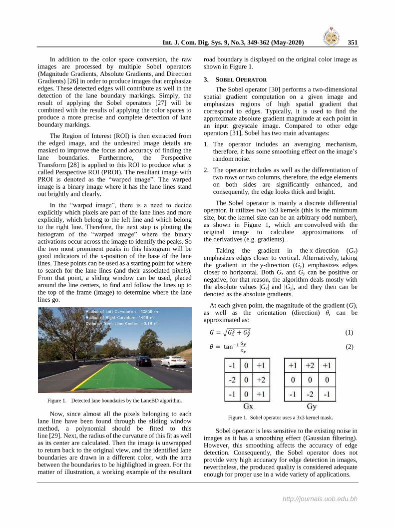
Figure 1. Detected lane boundaries by the LaneBD algorithm.

Now, since almost all the pixels belonging to each lane line have been found through the sliding window method, a polynomial should be fitted to this line [29]. Next, the radius of the curvature of this fit as well as its center are calculated. Then the image is unwrapped to return back to the original view, and the identified lane boundaries are drawn in a different color, with the area between the boundaries to be highlighted in green. For the matter of illustration, a working example of the resultant

road boundary is displayed on the original color image as shown in Figure 1.

3. SOBEL OPERATOR

The Sobel operator [30] performs a two-dimensional spatial gradient computation on a given image and emphasizes regions of high spatial gradient that correspond to edges. Typically, it is used to find the approximate absolute gradient magnitude at each point in an input greyscale image. Compared to other edge operators [31], Sobel has two main advantages:

1. The operator includes an averaging mechanism, therefore, it has some smoothing effect on the image’s random noise.

2. The operator includes as well as the differentiation of two rows or two columns, therefore, the edge elements on both sides are significantly enhanced, and consequently, the edge looks thick and bright.

The Sobel operator is mainly a discrete differential operator. It utilizes two 3x3 kernels (this is the minimum size, but the kernel size can be an arbitrary odd number), as shown in Figure 1, which are convolved with the original image to calculate approximations of the derivatives (e.g. gradients).

Taking the gradient in the x-direction (Gx) emphasizes edges closer to vertical. Alternatively, taking the gradient in the y-direction (Gy) emphasizes edges closer to horizontal. Both Gx and Gy can be positive or negative; for that reason, the algorithm deals mostly with the absolute values |Gx| and |Gy|, and they then can be denoted as the absolute gradients.

At each given point, the magnitude of the gradient (G), as well as the orientation (direction) θ, can be approximated as:

𝐺 = √𝐺𝑥2 + 𝐺𝑦

2 (1)

𝜃 = tan−1 𝐺𝑦

𝐺𝑥 (2)

Figure 1. Sobel operator uses a 3x3 kernel mask.

Sobel operator is less sensitive to the existing noise in images as it has a smoothing effect (Gaussian filtering). However, this smoothing affects the accuracy of edge detection. Consequently, the Sobel operator does not provide very high accuracy for edge detection in images, nevertheless, the produced quality is considered adequate enough for proper use in a wide variety of applications.

https://en.wikipedia.org/wiki/Kernel_(image_processing)#Convolution

https://en.wikipedia.org/wiki/Image_Derivatives



Usually, thresholds are used with the Sobel operator to identify the sharp edges from the weak ones (noise). Finding out the suitable threshold for each kind of gradient operator (Gx, Gy, G, θ) is critical for the proper application of this operator.

In the case of lane lines detection, the emphasis will be on the edges of a particular orientation. So the direction, or orientation, of the gradient as given by Eq. (2) here is of specific interest. After the application of the directional gradient, each pixel of the resulting image contains a value for the angle of the gradient away from the vertical axis in radians, covering a range of -π/2 → π/2. An orientation of 0 implies a vertical line and orientations of ± π/2 imply horizontal lines.

4. PERSPECTIVE TRANSFORM

A perspective transform maps the points in a given image to different and desired image points with a new perspective [32]. The perspective transform that is being most emphasized here, is a bird’s-eye view transform, which lets a lane be viewed from above. This particular view will be useful for fitting the lane polynomial and calculating more precisely the radius of the lane curvature. Aside from creating a bird’s eye view representation of an image, a perspective transform can also be used for all kinds of different viewpoints.

Figure 2 shows 4 points (𝑃1′, 𝑃2

′ , 𝑃3′ 𝑎𝑛𝑑 𝑃4

′) on a 2D plane to be transformed into their corresponding perspective points (P1, P2, P3, and P4). The perspective transformation is calculated in homogeneous coordinates and defined by a 3x3 matrix M. The calculation for a single point would be:

[

𝑀11 𝑀12 𝑀13

𝑀21 𝑀22 𝑀23

𝑀31 𝑀32 𝑀33

] ∗ [𝑃1

′. 𝑥

𝑃1′. 𝑦1

] = [𝑤 ∗ 𝑃1. 𝑥𝑤 ∗ 𝑃1. 𝑦

𝑤 ∗ 1] (3)

Figure 2. Perspective Transform of four points on a plane.

To calculate all points simultaneously, all the points are grouped together in one matrix A, and analogously for the transformed points in a matrix B, as follows in Eq. (4) and (5) respectively:

𝐴 = [𝑃1

′. 𝑥 𝑃2′ . 𝑥 𝑃3

′ . 𝑥

𝑃1′. 𝑦 𝑃2

′ . 𝑦 𝑃3′ . 𝑦

1 1 1

𝑃4′. 𝑥

𝑃4′. 𝑦1

] (4)

𝐵 = [𝑃1. 𝑥 𝑃2. 𝑥 𝑃3. 𝑥𝑃1. 𝑦 𝑃2. 𝑦 𝑃3. 𝑦

1 1 1

𝑃4. 𝑥𝑃4. 𝑦

1

] (5)

𝑀 = [

𝑀11 𝑀12 𝑀13

𝑀21 𝑀22 𝑀23

𝑀31 𝑀32 𝑀33

] (6)

𝑊 = [

𝑊1 0 00 𝑊2 00 0 𝑊3

000

0 0 0 𝑊4

] (7)

𝐵 ∗ 𝑊 = 𝑀 ∗ 𝐴 (8)

or 𝑀 = 𝐵 ∗ 𝑊 ∗ 𝐴−1 (9)

where W represents a scaling matrix that can be an identity matrix. Likewise, the inverse perspective transform (shown in Figure 3) can be implemented using the same technique as above.

Figure 3. Inverse Perspective Transform of four points on a plane.

5. MEASURING LANE CURVATURE

After extracting the pixels that belong to lane boundary (e.g. left and right lane-line segments shown in red and blue respectively in Figure 4) from the camera image, a polynomial can be fitted to those pixel positions to approximate lane boundaries in a concrete mathematical form as shown in Figure 4. Usually, 2nd or 3rd order polynomials are adopted for this approximation. Based on those polynomials, the radius of curvature of them will be computed [33].



Figure 4. Fit Left and Right lane lines with 2nd order polynomials.

The following equation represents the general form of 2nd order polynomial that approximate a curved lane line in a broader sense, where A, B, and C are the coefficients to be found by fitting the polynomial to the extracted lane-line pixel positions:

𝑓(𝑦) = 𝐴𝑦2 + 𝐵𝑦 + 𝐶 (10)

The variable “y” is used instead of “x” as the lane lines in the warped image are near vertical, and may have the same x value for more than one y value.

The radius of curvature at any arbitrary point x of the function “x=f(y)” is calculated as follows [25]:

𝑅𝑐𝑢𝑟𝑣𝑒 =[1+(

𝑑𝑥

𝑑𝑦)

2]

32

|𝑑2𝑥

𝑑𝑦2| (11)

In the case of the second-order polynomial as above, the first and second derivatives are given as follows:

𝑓′(𝑦) =𝑑𝑥

𝑑𝑦= 2𝐴𝑦 + 𝐵 (12)

𝑓′′(𝑦) =𝑑2𝑥

𝑑𝑦2 = 2𝐴 (13)

Therefore, the equation for the radius of curvature becomes:

𝑅𝑐𝑢𝑟𝑣𝑒 =(1+(2𝐴𝑦+𝐵)2)

32

|2𝐴| (14)

As shown in Eq. (14), the radius of curvature is a function of ’y’. As the ‘y’ values of the image increase from top to bottom, so if, for example, the radius of curvature closest to the vehicle needed to be measured, the formula above could be evaluated at the y value corresponding to the bottom of the image.

The computed radius of curvature is in pixels, however, to calculate it in actual units (meters) as the real world, a reference needs to be set in order to convert the dimensions in pixels to real dimensions in meters. This reference is selected to be the width of the lane. By knowing or measuring out the physical lane width, and comparing it with the projected one in warped images, the

conversion ratio can be determined. The US regulations [34] requires a minimum lane width of 12 feet or 3.7 meters, which also can be taken as the required reference. For example, if the measured width in the warped image is 700 pixels, then the conversion ratio will be 3.7/700 meter per pixel. This ratio can then be used to convert the radius of curvature from pixels to meters.

6. CAMERA CALIBRATION

The conversion from three dimensional (3D) real-world scene to a two dimensional (2D) one, exhibits by a camera, results in image distortion, as the transformation from 3D→2D is not perfect. Actually, the shape and size of objects get distorted (changed) in the resulting 2D image from the original 3D appearance. Therefore, before using the resulting 2D camera images, this distortion needs to be undone so that the correct and useful information can be extracted and analyzed.

The construction of real cameras includes using a curved lens to form an image. The light rays usually bend around the edges of these lenses with low or high degrees depends on the focus and position of objects. Therefore, distortion at the edges of the image happens, in a way that lines or objects appear to be more or less curved than their actual reality. This effect is called the “radial distortion”, and represents the principal source of distortion.

Moreover, there is another main source of distortion which is the “tangential distortion”. This distortion happens when the camera’s lens is not perfectly aligned parallel to the image plane that is associated with the camera sensor. This produces a tilt effect to the image, which shows objects nearer or farther away than they actually are.

There are three needed coefficients to correct for radial distortion: k1, k2, and k3. To correct the appearance of radially distorted points in an image, one can use a correction formula.

In the following equations Eq. (10), and Eq. (11), (x, y) is a point in a distorted image. To undistort these points, the first step is using OpenCV [35] to calculate r, which is the known distance between a point in an undistorted (corrected) image (xcorrected, ycorrected) and the center of the image distortion, which is often the center of that image (xc

, yc). This center point (xc, yc) is sometimes referred to as the distortion center. These points are illustrated below in Figure 5.

Figure 5. Points in a distorted and undistorted (corrected) images.



𝑥𝑑𝑖𝑠𝑡𝑜𝑟𝑡𝑒𝑑 = 𝑥𝑖𝑑𝑒𝑎𝑙 + (1 + 𝑘1𝑟2 + 𝑘2𝑟4 + 𝑘3𝑟6) (10)

𝑦𝑑𝑖𝑠𝑡𝑜𝑟𝑡𝑒𝑑 = 𝑦𝑖𝑑𝑒𝑎𝑙 + (1 + 𝑘1𝑟2 + 𝑘2𝑟4 + 𝑘3𝑟6) (11)

There are two more coefficients that account for tangential distortion: p1 and p2, and this distortion can be corrected using a different correction formula as given by Eq. (12) and (13).

𝑥𝑐𝑜𝑟𝑟𝑒𝑐𝑡𝑒𝑑 = 𝑥 + [2𝑝1𝑥𝑦 + 𝑝2(𝑟2 + 2𝑥2)] (12)

𝑦𝑐𝑜𝑟𝑟𝑒𝑐𝑡𝑒𝑑 = 𝑦 + [2𝑝1(𝑟2 + 2𝑦2) + 2𝑝2𝑥𝑦] (13)

To correct for the mentioned distortions, images of known shapes (chessboard images) are used. Selected points in the distorted plans are then mapped to undistorted plans as shown in Figure 6. Accordingly, the camera images will be calibrated. The following procedure is implemented to undistort the captured camera images and improve the image quality:

1) Step 1 – finding the chessboard corners: Using 20 chessboard images that have different sizes and orientations as depicted in Figure 7, the “cv2.findChessboardCorners()” function from the OpenCv3 library [35] is used to locate the chessboard corners. The detected number of corners is 9x6 as shown in the 17 out of the 20 images that are depicted in Figure 7. In the other 3 images, only 9x5 corners have been detected. The corners are drawn using the “cv2.drawChessboardCorners()” function of openCv3.

2) Step 2 – get camera matrices: A test chessboard image that has not been used before in finding the corners; is used; after being converted to a greyscale; along with the found corners in step one; to find the camera matrices. “cv2.CalibrateCamera()” function is used to perform this step. To check the quality of the calibration, the gray test image together with the camera matrices to remove the distortion of this image as shown in Figure 8.

Figure 6. Mapping from a distorted chessboard image to an undistorted

one.

Figure 7. Chessboard images used for calibration with corners drawn.

Figure 8. A test chessboard image with distortion removal.

3) Step 2 – saving camera matrices: using Pickle library [36], the camera data (the camera matrix as well as the distortion coefficients) are saved in the pickle file “camera_calibration.p” for easy retrieval later.

Figure 9 provides an example of applying the camera calibration procedure on one of the test images.

Figure 9. Camera calibration effect (undistortion of images).

7. IMAGE PROCESSING PIPELINE

The pipeline is implemented using Python and OpenCV computer vision library [35] and the following steps describe the implemented pipeline in order of execution:

1. HLS conversion: the images which are received in RGB color space are converted to HLS color space using the “cv2.cvtColor(img, cv2.COLOR_RGB2HLS)” OpenCV function. Then the “S” (saturation) channel is then extracted and stored in a specific image file. A threshold value of “170” is used to filter out weak associations with white or yellow color segments.

2. HSV conversion: the images which are received in RGB color space are converted to HSV color space using the “cv2.cvtColor(img, cv2.COLOR_RGB2HSV)” openCV function. Then, the “V” (value) channel is extracted.



3. LAB conversion: the RGB images are converted to LAB color space using the “cv2.cvtColor(img, cv2.COLOR_RGB2LAB)” OpenCV function. Then the “B” (color b) channel is then extracted and stored in a specific image file. A threshold value of “170” is used to filter out weak associations with yellow color segments as shown in Figure 10.

4. YUV conversion: the RGB images are converted to YUV color space using the “cv2.cvtColor(img, cv2.COLOR_RGB2YUV)” OpenCV function. Then the “Y” (color b) channel is then extracted and stored in a specific image file. A threshold value of “200” is used to filter out weak associations with white color segments as shown in Figure 11.

5. LUV conversion: the RGB images are converted to LUV color space using the “cv2.cvtColor(img, cv2.COLOR_RGB2LUV)” OpenCV function. Then the “L” (color b) channel is then extracted and stored in a specific image file. A threshold value of “200” is used to filter out weak associations with both white and yellow color segments as shown in Figure 10.

Figure 10. LUV (L-channel), and LAB (B-channel) images.

6. Absolute Sobel Gradients: the absolute Sobel gradient is implemented using the OpenCV “cv2.Sobel()” function. It is applied in the pipeline for both the x and y-axis. The used minimum and maximum thresholds for the Sobelx is ‘20’ and ‘200’ respectively. Moreover, the used minimum and maximum threshold for the Sobely is ‘150’ and ‘180’ respectively.

7. Magnitude Sobel Gradients: the magnitude Sobel gradient is implemented from the results of applying Sobel gradients on both the x and y-axis, by using Eq. (1). It is applied in the pipeline with a kernel value of ‘9’. The used minimum and maximum thresholds are ‘100’ and ‘200’ respectively.

8. Direction Sobel Gradients: the direction Sobel gradient is implemented from the results of applying Sobel gradients on both the x and y-axis, by using Eq. (2). It is applied in the pipeline with a kernel value of ‘3’. The used minimum and maximum thresholds are ‘0.7’ and ‘1.3’ radians respectively.

9. Color Extraction in RGB images: White color is masked as well by filtering the RGB color space using thresholds of “202→255” for the three color channels. Moreover, the yellow color is masked by filtering the HSV color space using thresholds of “20→38” on the “H” channel, “60→174” on the “S” channel and

“60→250” on the “V” channel. The resultant binary image of the combined white any yellow filtering is shown below in Figure 12. Additionally, the resultant image of all the techniques combined is shown in the same figure.

10. Combining All: After applying the above operations, the combined results produces an output represented by Figure 12.

Figure 11. YUV (Y-channel), and “Sobel + Color Mapping” images.

Figure 12. White and Yellow Masked, and the Combined Techniques

images.

8. THE LANE-BOUNDARY DETECTION PIPELINE

Like the previous one, this pipeline is also implemented using Python and OpenCV computer vision library [31], and the following steps describe the implemented pipeline in order of execution:

1. Undistorting the image: removing the distortion of the captured images using the described technique in Section 6. Figure 9 shows the effect before and after the execution.

2. Applying the image processing pipeline: the image processing pipeline described in Section 7 is executed sequentially. The resultant binary image is shown in Figure 12. The results are due to the several color masking and extraction techniques as well as applying multiple Sobel operators (Absolute (x and y), Magnitude & Direction).

3. Identifying the region of Interest (ROI): after exhaustive trials and errors, the region of interest has been identified and applied to the resulting image of step 2 as shown in Fig. 13. The vertices of the ROI are: the upper-left => (620, 420), the upper-right => (680, 420), the lower-right => (1200, 720), and the lower-left => (150, 720).



Fig. 13 Identification and application of the Region of Interest.

4. Mask the undesired image details: The regions other than the region of interest are then masked (as shown in Figure 14) to give the LaneBD algorithm more focus.

5. Identifying and applying the Perspective Region of Interest (PROI): after exhaustive trials and errors, the perspective region of interest has been identified and applied on (warping) the resulting image of step 1 (the undistorted image) as shown in 0. The vertices of the PROI are: the upper left => (575, 465), the upper right => (010, 465), the lower right => (1050, 680), and the lower-left => (260, 680).

6. Applying Sliding Windows Search and Fit Polynomials: A sliding windows search algorithm has been implemented. The algorithm takes the “Warped PROI image” (shown in Figure 15) and produces the histogram and the left and right fit polynomials shown in Figure 16. The purpose of this step is the initial identification of lane lines points.

Figure 14. Masking other than the Region of Interest.

Figure 15. Identification and application of the Perspective Region of

Interest.

7. Applying Recursive Search: A recursive fine search algorithm has been implemented. The algorithm takes the “Warped PROI image” (shown in Figure 15) and the initial left and right polynomial coefficients found in

step 6, or from the previous iteration (recursive), and produces the refined left and right fit polynomials as shown in Figure 17. The purpose of this step is essentially the recursive identification of lane lines points, which consumes less computational overhead than the windows based one.

Figure 16. Histogram and sliding window search and the fitting left and

right lane polynomials.

8. Measuring lane curvature and center: the curvature of both the left and right lanes is then calculated as well as the position of the car with respect to the center of the lane. These calculations have been performed as per the description in Section 5.

9. Unwarping the image: the resulting image from step 7 (Figure 17) is being unwrapped using the “cv2.warpPerspective()” function and the calculated inverse warp Matrix “Minv” from step 5.

10. Highlight the identified lane: as the final step in the finding lanes pipeline, the unwrapped lane lines are drawn back on the undistorted image (Figure 9) with the area between the identified lane lines been highlighted in green as shown in Figure 18. The values of the lane curvatures and the distance of the car from the lane center is printed at the top of the image.

Figure 17. Recursive fine search and the fitting left and right lane

polynomials.



Figure 18. Identified lane lines highlighted in green and the measured

lane curvatures.

9. PARAMETER TUNING

The parameters of the LaneBD pipeline can be categorized into three main categories: the color-spaces category, the Sobel-operators category, and the region-of-interest category. The following analysis shed the light on the procedures used to find and fine-tune these parameters.

1.1. Setting the parameters of color spaces

The LaneBD algorithm uses several color spaces to extract the road-lines segments from road images. Filtering the selected color spaces requires setting several parameters to effectively extract the lanes segments either “white” or “yellow”. In this work, the white road-lines segments are extracted from: 1) The S channel of HLS, 2) The V channel of HSV, 3) The Y channel of YUV, 4) The L channel of LUV, 5) The R, G, and B channels of RGB. Likewise, the yellow road-lines segments are extracted from: 1) The S channel of HLS, 2) The V channel of HSV, 3) The B channel of LAB, 4) The L channel of LUV, 5) The R, G, and B channels of RGB.

The multiple filters (e.g. 5 filters) used for the extraction of each color are strengthening each other to improve the robustness of the algorithm. The filters parameters (mainly threshold values) are set and tuned using a guided trial-and-error procedure. In the following steps, the procedure is illustrated in the HLS color space (as an example):

1. Convert several test images (like the ones in Fig. 21 → Fig. 28) from RGB to HLS color space using the “cv2.cvtColor(img, cv2.COLOR_RGB2HLS)” OpenCV function.

2. Isolate the 3 channels of the HLS (Hue, Lumination, and Saturation) and save them in three separate channel images using the “cv2.inRange(hls, lower, upper)” OpenCV function.

3. An inspection software tool is developed to allow displaying the values of a certain pixel (either hue, lumination, or saturation) of the selected image, after moving the cursor on this pixel and clicking on it.

4. By visual inspection of the resulted channel images, and directing the cursor towards the areas of lane-lines segments, the feasible range of values of the “hue”, “lumination”, and “saturation” of the segments can be determined.

5. Based on these observations, it is found that the “S” channel is the most effective in isolating both the white and yellow segments than the other channels. Therefore, only the “S” channel images are kept and the other channel images are discarded.

6. A threshold is created to filter out weak associations with white or yellow color segments. After several trials-and-errors experimentations, the threshold is fine-tuned to “170”.

The above procedure is repeated to tune the parameters of the other color spaces LAB, HSV, YUV, RGB, etc. additionally, these threshold values are inserted in the header files of the code so they can be tweaked as needed.

1.2. Setting the parameters of Sobel Operators

All the Sobel operators (Absolute, Magnitude, and Direction) depend on thresholds’ values to filter out the noise and weak gradients in order to provide robust edge detection functionality. In this work, finding out the optimal (or in other words, the most suitable) threshold value for each operator is done through a guided trial-and-error procedure. The guidance is carried out using a numerical performance indicator developed based on Tsallis entropy [37]. The optimal threshold value t* can be found by [38]

𝑡∗(𝑞) = 𝐴𝑟𝑔𝑡∈𝐺𝑚𝑎𝑥[𝑆𝑞𝐴(𝑡) + 𝑆𝑞

𝐵(𝑡) + (1 −

𝑞). 𝑆𝑞𝐴(𝑡). 𝑆𝑞

𝐵(𝑡)] (14)

where t is an arbitrary luminance level (threshold value), G is the set of all grayscale levels {0,1,2, … ,255}, “A” denotes class A that represents the pixels associated with the background of the image, and “B” denotes class B that represents the pixels associated with the edges in the image. 𝑆𝑞

𝐴 is the Tsallis entropy of class A of order q.

Likewise, 𝑆𝑞𝐵 is the Tsallis entropy of class B of order q.

The Threshold Tuning procedure to select the most suitable (i.e. optimal) threshold value t* and q can now be described as follows:

Procedure Threshold Tuning,

Input: An RGB color image “C” of size M×N×3. Output: The suitable threshold t* value of “C”, for q ≥ 0.

Begin 1. Convert“C” to a grayscale image “A” of size

M×N. 2. Let f(x, y) be the original gray value of the pixel at

the point (x, y), x=1... M, y=1… N. 3. Construct the histogram h(i) for i ∈ G from all the

pixels of image “A”.



4. Calc. the probability distribution 𝑝𝑖 =ℎ(𝑖)

𝑀×𝑁 , 𝑖 ∈ 𝐺.

5. For all t ∈ G i. Construct the probability distribution set of class

A: 𝑝𝐴 = {𝑝0

𝑃𝐴,

𝑝1

𝑃𝐴, … ,

𝑝𝑡

𝑃𝐴 }, where 𝑃𝐴 = ∑ 𝑝𝑖

𝑡𝑖=0 .

ii. Construct the probability distribution set of class

B: 𝑝𝐵 = {𝑝𝑡+1

𝑃𝐵,

𝑝𝑡+2

𝑃𝐵, … ,

𝑝255

𝑃𝐵 }, where 𝑃𝐵 =

∑ 𝑝𝑖255𝑖=𝑡+1 .

iii. Calculate the entropy of order q for class A:

𝑆𝑞𝐴(𝑡) =

1

𝑞−1(1 − ∑ (𝑝𝐴

𝑖 )𝑞𝑡

𝑖=0 ).

iv. Calculate the entropy of order q for class B:

𝑆𝑞𝐵(𝑡) =

1

𝑞−1(1 − ∑ (𝑝𝐵

𝑖 )𝑞255

𝑖=𝑡+1 ).

v. Calculate the entropy of order q: 𝑆𝑞(𝑡) =𝑆𝑞

𝐴(𝑡) + 𝑆𝑞𝐵(𝑡) + (1 − 𝑞). 𝑆𝑞

𝐴(𝑡). 𝑆𝑞𝐵(𝑡).

6. 𝑡∗(𝑞) = 𝐴𝑟𝑔𝑡∈𝐺𝑚𝑎𝑥[𝑆𝑞(𝑡)] End.

The above procedure should be repeated several times for different values of q. In this work, values from 0.25 → 4.0 have been tried following the work in [37], and finally, q = 3.0 is selected. The above procedure is also used to find all the threshold values for all Sobel operators.

1.3. Selecting the Region of Interest (ROI) vertices

To make the LaneBD robust and computationally effective, the portion of the image which includes the lane lines should only be considered. This portion is determined by finding the horizon (i.e. the projected intersection of the left and right lane line segments, when determined, is referred to as the horizon). By examining many camera images, the region of interest is found to be the lower 60% of the examined images. To be more specified and focus only on the front drivable lane, not any other neighboring lanes, therefore, the ROI used by the LaneBD takes the form of a trapezoidal shape not a rectangular. Based on a camera image of size 1200×720, the identified ROI vertices are: the upper left => (620, 420), the upper right => (680, 420), the lower right => (1200, 720), and the lower-left => (150, 720) as shown in Figure 16.

10. TESTING AND VALIDATION

The developed LaneBD algorithm is further tested on many images representing different scenarios. Samples of the results of the testing are shown in Figure 19, Figure 20, Figure 21, Figure 22, Figure 23 and Figure 24. The presented results show that the algorithm performs very well under different conditions (at full sunrise, at sunset, with shadows, without shadows, with cars on the other lanes and without). Furthermore, for robustness testing and validation of the developed pipeline, the algorithm is applied to several real-time video samples representing different driving conditions. The LaneBD proved to be very robust in all the pre-mentioned conditions. However, the scattered areas of shadows have some effect on the precision of producing the lane boundaries as shown in

Figure 22. However, the output is still acceptable and produce functional results.

The pipeline proved to be acceptably fast in execution to be used in real-time. Using an Intel Core i5 with 1.6 GHz and 8 GB RAM which is a very moderate computational platform, the following measurements (Table 1) are collected for two testing video streams:

TABLE 1 COMPUTATION SPEED FOR THE LANEBD ALGORITHM.

Sample Name No. of Frames

Total Time Min:Sec

Frame per Sec

Challenge Video 485 00:46 10.70

Project Video 1261 02:05 10.12

The lowest measured processing speed is 10 Frames Per Second (FPS), which is considered just adequate as per the recommended performance for this application [39]. However, more powerful computational hardware is required to promote the presented real-time performance [40], which mandates testing the performance with GPUs.

The pipeline is executed as well on google Colab cloud platform [41] in three different modes: CPU (Intel Xeon Processor @2.3GHz (1 core, 2 threads), 13GB RAM), GPU (NVIDIA Tesla K80, 13GB RAM) and TPU (v2) [41]. Table 2 shows the results of these trials indicating that not much difference in performance is taking place compared to the previous results. The existence of the GPU added only an improvement of 17% in computational speed, while the TPU is adding only 1.5%. The justification for these results is that the GPU is mainly speeding the matrix operations and the developed pipeline does involve much of matrix operations. Moreover, the TPU is mainly designed to speed up computation based on tensors which are not used in the formulation of the LaneBD algorithm.

TABLE 2 COMPUTATION SPEED ON GOOGLE COLAB.


FPS CPU

FPS GPU

FPS TPU

Challenge Video 485 11.70 13.90 11.94

Project Video 1261 11.42 13.43 11.54

Harder Challenge

Video 1200 10.08 12.03 10.35

Challenge 251 10.93 12.51 11.11

SolidWhiteRight 222 11.38 13.04 11.51

SolidYellowLeft 682 11.56 13.64 11.56



Figure 19. Test image with solid yellow and dotted white lane lines

(bright sunny road (at noon), left lane with cars).

The LaneBD is compared with the LaneRTD algorithm proposed in [42]. The LaneRTD is mainly based on Canny edge detection [18] followed by Hough transform [14]. The results in Table 3 show that LaneRTD algorithm is faster as it utilizes much simpler pipeline, however, in terms of robustness, the current LaneBD, which is a more complex and comprehensive pipeline, is significantly more robust especially in unfavorable conditions like scattered shadows as shown by the comparison between Figure 22 and Fig. 28.

TABLE 3 SPEED COMPARISON BETWEEN LANERTD AND LANEBD.


FPS LaneRTD

FPS LaneBD

Challenge 251 10.93 12.51

SolidWhiteRight 222 25.60 13.04

SolidYellowLeft 682 18.76 13.64


segments (road at sunset (dusk), left lane with no cars).


segments (left turning lane at dusk with cars).


segments (left turning lane with scattered shadows, and cars) using

LaneBD.


segments (left turning lane with scattered shadows, and cars).



Figure 24. Test image with solid while and dotted white lane lines

segments (right straight lane at sunset, and no cars).


segments (left turning lane with scattered shadows, and cars) using

LaneRTD [43].

11. TESTING AND VALIDATION

The following points shed some light on some technical tricks and aspects that have been tried or implemented in the described pipelines:

1) HSV color space: The channels H, S and V, have been extracted and tried to investigate the worthiness of adding any of them to the final overall combination. However, we find out that the S channel is exactly the same as the one in the HSL color space, so no need for duplication. The H and V channels, when got combined separately or together with the overall combination, do not add significant value to the final result or sometimes they make it worse. As a result, it has been decided not to integrate the HSV color space in the final combination.

2) S-channel of HLS: It is observed that using the S channel in the final pipeline, causes jittering in video streams especially in areas with fragmented shades. Therefore, using it in the pipeline could be avoided.

3) B-channel of LAB: The B channel of the LAB color space; has proved very effective in extracting the yellow color or in other words the yellow segments as shown in Figure 10.

4) L-channel of LUV: The L channel of the LUV color space; has proved very effective as well in extracting both the white and the yellow lane lines as shown in Figure 10.

5) Y-channel of YUV: The Y channel of the YUV color space; has proved very effective in extracting the white lane lines as shown in Figure 11.

6) Perspective Region Of Interest (PROI): some trials are carried out to define the lane region of interest of the image (ROI) the same as the perspective region of interest (PROI). However, these trials were not successful, and it has been decided to define them separately for accurate perspective transformation.

7) Sanity Checks: several sanity checks, have been used throughout the pipeline, trying to prevent bad lines from reaching the final image. The following are a list of them:

a) Order of the fitted left and right lines: in order to ensure that the fitted left and right polynomials have intercepts with the x-axis in the right order, this check is implemented in the code.

b) Update of the left and right lines: during video testing, both the right and left lane polynomial coefficients are getting updated each frame. Logically, the change of these coefficients should be small and if it is found big, this indicated that this line fit is not good enough and should be discarded. This check is done for the left and right lane separately in the implemented code.

c) Check on the right and left lanes curvatures: logically, the right and left lanes radius of curvatures should be almost identical all the time. However, doing these checks to separate good and bad line fits proved very tricky especially when the actual lane lines are vertical with no curves. The use of this method is not robust and can result in the rejection of many good lines. Therefore, it is not applied.

8) Applying Resets: the initial lane line fits is being determined using the sliding windows search function mentioned in step 6 of the pipeline in Section 8. Then, the recursive fine search function; that is mentioned in step 7 of the pipeline; kicks in to calculate the line fits for the next frames. However, after several frames, the estimation errors accumulate, and the found lines diverge and become unrealistic. For this reason, the sliding windows function has to be utilized again to determine the lane lines from the raw undistorted images. In order to avoid this problem, and to make this procedure more systematic, a reset procedure is being adopted. For each number of frames (determined by trial and error, and has been set to “8” in the current implementation), the sliding windows function kicks in and then followed by the recursive search function for several frames. In our current code, “the reset span = 8”,



which means that the sliding windows function will work for the first frame and then followed by a recursive search function for the next 7 frames, and so on, etc. This implemented technique works very well to avoid divergence and at the same time, reduces the video processing time.

9) Smoothing using FIR filtering: after calculating the left or the right fit polynomials on a certain frame, instead of using it directly, we average the results over the last 3 samples to smooth out the determined values and reduces noise and unexpected jitters in directions [44]. This step is done for both the left and right lanes in the implemented code.

10) Lanes data acquisition: In order to perform a thorough analysis of the results, a class (data structure) called “Line()” has been constructed and used in the code. Using this class, several useful information has been recorded regarding the fitted left and right lanes. The collected information proved very effective in many tasks of the pipeline like “smoothing and FIR filtering”, “sanity checks” … etc.

12. CONCLUSION

In this paper, a reliable-and-sophisticated lane-boundaries detection-and-tracking solution based on computer-vision algorithms is developed, presented thoroughly and given the name LaneBD. The main contribution of the LaneBD algorithm is the sophisticated fusion of color spaces such as LAB, YUV, LUV, etc., and computer-vision algorithms like Sobel operators and Perspective Transform to produce a robust fast output. Additionally, the pipeline uses a comprehensive image distortion suppression and camera calibration techniques to produce undistorted road images suitable for more accurate lane detection. Moreover, several sanity-check tricks are exercised to improve the robustness of the techniques used. The proposed LaneBD technique needs only raw RGB images from a single CCD camera mounted behind the front windshield of the vehicle. The performance of the LaneBD is tested and evaluated using many stationary images and several real-time videos. The validation results show a fairly accurate and robust detection with slight insignificant deviation in one scenario where complex shadow patterns exist. The measured throughput (execution time) using an affordable CPU proved that the LaneBD is very suitable for real-time lane detection. Therefore, the proposed technique is well suited for use in advanced driving assistance systems or self-driving cars. A comprehensive discussion and analysis regarding the usefulness and the shortcomings of the proposed technique are presented.

ACKNOWLEDGMENT

This work used the High-Performance Computing (HPC) facilities of the American University of the Middle East, Kuwait.

REFERENCES

[1] Wael Farag, “Traffic signs classification by deep learning for advanced driving assistance systems”, Intelligent Decision Technologies, IOS Press, vol. 13, no. 3, pp. 215-231, (2019).

[2] Wael Farag, Zakaria Saleh, "Road Lane-Lines Detection in Real-Time for Advanced Driving Assistance Systems", Intern. Conf. on Innovation and Intelligence for Informatics, Computing, and Technologies (3ICT'18), Bahrain, 18-20 Nov., (2018).

[3] Wael Farag, Zakaria Saleh, "Behavior Cloning for Autonomous Driving using Convolutional Neural Networks”, Intern. Conf. on Innovation and Intelligence for Informatics, Computing, and Technologies (3ICT'18), Bahrain, 18-20 Nov., (2018).

[4] Wael Farag, “Recognition of traffic signs by convolutional neural nets for self-driving vehicles”, International Journal of Knowledge-based and Intelligent Engineering Systems, IOS Press, vol. 22, no: 3, pp. 205 – 214, (2018).

[5] Wael Farag, Zakaria Saleh, "Tuning of PID Track Followers for Autonomous Driving", Intern. Conf. on Innovation and Intelligence for Informatics, Computing, and Technologies (3ICT'18), Bahrain, 18-20 Nov., (2018).

[6] Wael Farag, “Safe-driving cloning by deep learning for autonomous cars”, International Journal of Advanced Mechatronic Systems, Inderscience Publishers, vol. 7, no. 6, pp. 390-397, (2019).

[7] Wael Farag and Zakaria Saleh, “An Advanced Vehicle Detection and Tracking Scheme for Self-Driving Cars”, 2nd Smart Cities Symposium (SCS’19), IET Digital Library, Bahrain, 24-26 March, (2019).

[8] Wael Farag and Zakaria Saleh, “MPC Track Follower for Self-Driving Cars”, 2nd Smart Cities Symposium (SCS’19), IET Digital Library, Bahrain, 24-26 March, (2019).

[9] Wael Farag, Z. Saleh, "An Advanced Road-Lanes Finding Scheme for Self-Driving Cars", Smart Cities Symposium (SCS'19), IET Digital Library, Bahrain, 24-26 March, (2019).

[10] B. M, Broggi, “GOLD: A parallel real-time stereo vision system for generic obstacle and lane detection”, IEEE Transactions on Image Processing, 1998, pp. 4-6.

[11] C. Kreucher, S. K. Lakshmanan, “A Driver warning System based on the LOIS Lane Detection Algorithm”, in the IEEE Intern. Conf. On Intelligent Vehicles, Stuttgart, Germany, 1998, pp. 17 -22.

[12] M. Chen., T. Jochem D. T. Pomerleau, “AURORA: A Vision-Based Roadway Departure Warning System”, in the IEEE Conference on Intelligent Robots and Systems, 1995.

[13] B. Ran and H. Xianghong, “Development of A Vision-based Real-Time lane Detection and Tracking System for Intelligent Vehicles”, In 79th Annual Meeting of Transportation Research Board, Washington DC, 2000.

[14] R.O. Duda, and P. E. Hart, "Use of the Hough Transformation to Detect Lines and Curves in Pictures”, Comm. ACM, Vol. 15, pp. 11–15 (January 1972).

[15] A. Assidiq, O. Khalifa, M. Islam, S. Khan, “Real-time lane detection for autonomous vehicles”, in the Intern. Conf. on Computer and Communication Eng., May 13-15, 2008 Kuala Lumpur, Malaysia.

[16] M. Aziz, A. Prihatmanto, and H. Hindersah, “Implementation of lane detection algorithm for self-driving car on toll road cipularang using Python language”, 4th Intern Conf. on Electric Vehicular Technology (ICEVT), Bali, Indonesia, Oct. 2017.

[17] Wikipedia, https://en.wikipedia.org/wiki/Canny_edge_detector, (retrieved 8/23/18).

[18] J. Canny, “A Computational Approach To Edge Detection”, IEEE Trans. Pattern Analysis and Machine Intelligence, 8(6):679–698, 1986.

https://www.inderscienceonline.com/doi/abs/10.1504/IJAMECHS.2017.099318

https://www.inderscienceonline.com/doi/abs/10.1504/IJAMECHS.2017.099318

https://en.wikipedia.org/wiki/Canny_edge_detector



[19] Jasmine Wadhwa, G.S. Kalra and B.V. Kranthi, “Real-Time Lane Detection in Autonomous Vehicles Using Image Processing”, Research Journal of Applied Sciences, Engineering and Technology 11(4): 429-433, 2015. DOI: 10.19026/rjaset.11.1798.

[20] Wael A Farag, VH Quintana, G Lambert-Torres, “Genetic algorithms and back-propagation: a comparative study”, IEEE Canadian Conf. on Elec. and Comp. Eng., vol. 1, pp. 93-96, Waterloo, Ontario, Canada, (1998).

[21] S. Lee, I. Kweon, J. Kim, J. Yoon, S. Shin, O. Bailo, N. Kim, T.-H. Lee, H. Hong, and S.-H. Han, “Vpgnet: Vanishing point guided network for lane and road marking detection and recognition”, In 2017 IEEE Intern. Conf. on Computer Vision (ICCV), pp. 1965–73., 2017.

[22] J. Li, X. Mei, D. Prokhorov, and D. Tao, “Deep neural network for structural prediction and lane detection in traffic scene”, IEEE Transactions on Neural Networks and Learning Systems, 28(3):690–703, 2016.

[23] X. Dong, Z. Yu, W. Cao, Y. Shi, QianliMA, “A survey on ensemble learning”, Frontiers of Computer Science, Springer, August, (2019).

[24] “Color Space”, https://en.wikipedia.org/wiki/Color_space, retrieved on 15th Sept. 2018.

[25] “List of color spaces and their uses”, https://en.wikipedia.org/wiki/List_of_color_spaces_and_their_uses, retrieved on 15th Sept. 2018.

[26] R. Duda and P. Hart, “Pattern Classification and Scene Analysis”, John Wiley and Sons, 1973, pp. 271-2.

[27] Irwin Sobel, 2014, “History and Definition of the Sobel Operator”, https://www.researchgate.net/publication/239398674_An_Isotropic_3_3_Image_Gradient_Operator, retrieved on 15th Sept. 2018.

[28] Ingrid Carlbom, Joseph Paciorek, "Planar Geometric Projections and Viewing Transformations", ACM Computing Surveys, 10 (4): 465–502, (1978), DOI:10.1145/356744.356750

[29] “Polynomial regression”, https://en.wikipedia.org/wiki/Polynomial_regression, retrieved on 16th Sept. 2018.

[30] I. Sobel, “An isotropic 3×3 gradient operator,” in Machine Vision for Three-Dimensional Scenes, H. Freeman, Ed., pp. 376–379, Academic Press, New York, NY, USA, 1990.

[31] Raman Maini, Himanshu Aggarwal, “Study and Comparison of Various Image Edge Detection Techniques”, Intern J. of Image Processing (IJIP), Vol. 3, Issue 1, 2009.

[32] S. Tan, J. Dale, A. Anderson, A. Johnston, “Inverse Perspective Mapping and Optic Flow: A Calibration Method and a Quantitative Analysis”, Image Vision Comput. 2006, 24, 153-165.

[33] “Radius of Curvature”, https://www.intmath.com/applications-differentiation/8-radius-curvature.php, retrieved on (24 Sept. 2018).

[34] “U.S. government specifications for highway curvature”, http://onlinemanuals.txdot.gov/txdotmanuals/rdw/horizontal_alignment.htm#BGBHGEGC, retrieved on (26 Sept. 2018).

[35] OpenCV Python Library, https://opencv.org/.

[36] “Python Pickle Module”, https://docs.python.org/3.1/library/pickle.html, retrieved on (24 Sept. 2018).

[37] MP De Albuquerque, IA Esquef, ARG Mello, “Image thresholding using Tsallis entropy”, Pattern Recognition Letters, Elsevier, vol. 25 (9), pp. 1059-1065, (2004).

[38] M. A. El-Sayed, “A New Algorithm Based Entropic Threshold for Edge Detection in Images”, IJCSI International Journal of Computer Science Issues, Vol. 8, Issue 5, No 1, September, (2011).

[39] Jan Botsch, “Real-time lane detection and tracking on high-performance computing devices”, Bachelor's Thesis in Informatics, Technische Universitat, Munchen, Germany, March 2015.

[40] M. Nagiub and W. Farag, “Automatic selection of compiler options using genetic techniques for embedded software design”, IEEE 14th Inter. Symposium on Comp. Intelligence and Informatics (CINTI), Budapest, Hungary, Nov. 19, (2013).

[41] “Google Colaboratory”, https://colab.research.google.com/notebooks/welcome.ipynb, accessed on (5 April 2019).

[42] Wael Farag and Zakaria Saleh, “Road Lane-Lines Detection in Real-Time for Advanced Driving Assistance Systems”, Intern. Conf. on Innovation and Intelligence for Informatics, Computing, and Technologies (3ICT 2018), Bahrain, 18-20 Nov., 2018.

[43] Wael Farag, “Real-Time Detection of Road Lane-Lines for Autonomous Driving”, Recent Patents on Computer Science, Bentham Science Publishers, Vol. 12, Issue 4, 2019.

[44] Wael Farag, Ahmed Tawfik, “On fuzzy model identification and the gas furnace data”, Proceedings of the IASTED International Conference Intelligent Systems and Control, Honolulu, Hawaii, USA, August 14-16, (2000).

Wael Farag earned his Ph.D. from

the University of Waterloo, Canada

in 1998; M.Sc. from the University

of Saskatchewan, Canada in 1994;

and B.Sc. from Cairo University,

Egypt in 1990. His research,

teaching and industrial experience

focus on embedded systems,

mechatronics, autonomous vehicles,

renewable energy, and control

systems. He has combined 17 years

of industrial and senior management experience in Automotive

(Valeo), Oil & Gas (Schneider) and Construction Machines

(CNH) positioned in several countries including Canada, USA &

Egypt. Moreover, he has 10 Years of academic experience at

Wilfrid Laurier University, Cairo University, and the American

University of the Middle East. Spanning several topics of

electrical and computer engineering. He is the holder of 2 US

patents; ISO9000 Lead Auditor Certified and Scrum Master

Certified.

https://en.wikipedia.org/wiki/Color_space

https://en.wikipedia.org/wiki/List_of_color_spaces_and_their_uses

https://en.wikipedia.org/wiki/List_of_color_spaces_and_their_uses

https://www.researchgate.net/publication/239398674_An_Isotropic_3_3_Image_Gradient_Operator

https://www.researchgate.net/publication/239398674_An_Isotropic_3_3_Image_Gradient_Operator

https://en.wikipedia.org/wiki/Digital_object_identifier

https://doi.org/10.1145/356744.356750

https://en.wikipedia.org/wiki/Polynomial_regression

https://www.intmath.com/applications-differentiation/8-radius-curvature.php

https://www.intmath.com/applications-differentiation/8-radius-curvature.php

http://onlinemanuals.txdot.gov/txdotmanuals/rdw/horizontal_alignment.htm#BGBHGEGC

http://onlinemanuals.txdot.gov/txdotmanuals/rdw/horizontal_alignment.htm#BGBHGEGC

https://opencv.org/

https://docs.python.org/3.1/library/pickle.html

https://colab.research.google.com/notebooks/welcome.ipynb

Date post:	05-Dec-2021
Category:	Documents
Upload:	others
View:	2 times
Download:	0 times

A Comprehensive Real-Time Road-Lanes Tracking Technique ...

Documents