DOI 10.1140/epjp/i2014-14013-7 Regular Article Eur. Phys. J. Plus (2014) 129: 13 T HE EUROPEAN P HYSICAL JOURNAL PLUS A computational study of entropy generation in magnetohydrodynamic flow and heat transfer over an unsteady stretching permeable sheet Adnan Saeed Butt a and Asif Ali Department of Mathematics, Quaid-i-Azam University Islamabad, Pakistan Received: 9 July 2013 / Revised: 4 December 2013 Published online: 30 January 2014 – c Societ` a Italiana di Fisica / Springer-Verlag 2014 Abstract. The present article aims to investigate the entropy effects in magnetohydrodynamic flow and heat transfer over an unsteady permeable stretching surface. The time-dependent partial differential equations are converted into non-linear ordinary differential equations by suitable similarity transformations. The solutions of these equations are computed analytically by the Homotopy Analysis Method (HAM) then solved numerically by the MATLAB built-in routine. Comparison of the obtained results is made with the existing literature under limiting cases to validate our study. The effects of unsteadiness parameter, magnetic field parameter, suction/injection parameter, Prandtl number, group parameter and Reynolds number on flow and heat transfer characteristics are checked and analysed with the aid of graphs and tables. Moreover, the effects of these parameters on entropy generation number and Bejan number are also shown graphically. It is examined that the unsteadiness and presence of magnetic field augments the entropy production. 1 Introduction During the last three decades, one of the major interests of scientists and engineers is to increase the efficiency of thermal and mechanical systems. This can be achieved by reducing the loss of useful energy in these systems. Especially in heat transfer and flow processes, destruction of useful energy results in reducing the thermal and mechanical efficiency of the system. This can cause great disorder in the system which can be measured in terms of entropy generation. It is a tool which can be used to study the irreversibility effects in the system. The pioneer work in this field was done by Bejan [1] who focussed on different reasons behind entropy production. Sources like heat transfer along a temperature gradient, convective heat transfer, viscous dissipation, thermal radiation etc., are responsible for generation of entropy. Since then, researchers have made numerous investigations to examine the entropy effects for different geometrical configurations [2–19]. Boundary layer flow and heat transfer over a stretching surface have been extensively studied due to their wide applications in industrial and manufacturing processes such as extrusion of plastic sheets, paper production, crystal growing, etc. Much literature is available on steady flow and heat transfer over a stretching sheet, some of which is cited in refs. [20–25]. However, the unsteady flow phenomenon is a bit complicated and less literature is available as compared to the steady flow [26–32]. The present article focusses on investigating the entropy effects in unsteady flow and heat transfer over a permeable stretching sheet. The cause of unsteadiness in flow and temperature fields is the time dependence of stretching velocity and surface temperature. A complete parametric study has been done and the results are presented through graphs and tables. 2 Mathematical formulation Consider a two-dimensional laminar boundary layer flow of an electrically conducting viscous fluid due to the stretching of a porous sheet. Keeping the origin fixed, the sheet is stretched along the x-axis with velocity U w (x, t), whereas the a e-mail: [email protected]
Transcript
DOI 10.1140/epjp/i2014-14013-7
Regular Article
Eur. Phys. J. Plus (2014) 129: 13 THE EUROPEANPHYSICAL JOURNAL PLUS
A computational study of entropy generation inmagnetohydrodynamic flow and heat transfer over anunsteady stretching permeable sheet
Adnan Saeed Butta and Asif Ali
Department of Mathematics, Quaid-i-Azam University Islamabad, Pakistan
Abstract. The present article aims to investigate the entropy effects in magnetohydrodynamic flow and heattransfer over an unsteady permeable stretching surface. The time-dependent partial differential equationsare converted into non-linear ordinary differential equations by suitable similarity transformations. Thesolutions of these equations are computed analytically by the Homotopy Analysis Method (HAM) thensolved numerically by the MATLAB built-in routine. Comparison of the obtained results is made withthe existing literature under limiting cases to validate our study. The effects of unsteadiness parameter,magnetic field parameter, suction/injection parameter, Prandtl number, group parameter and Reynoldsnumber on flow and heat transfer characteristics are checked and analysed with the aid of graphs andtables. Moreover, the effects of these parameters on entropy generation number and Bejan number arealso shown graphically. It is examined that the unsteadiness and presence of magnetic field augments theentropy production.
1 Introduction
During the last three decades, one of the major interests of scientists and engineers is to increase the efficiency of thermaland mechanical systems. This can be achieved by reducing the loss of useful energy in these systems. Especially inheat transfer and flow processes, destruction of useful energy results in reducing the thermal and mechanical efficiencyof the system. This can cause great disorder in the system which can be measured in terms of entropy generation. It isa tool which can be used to study the irreversibility effects in the system. The pioneer work in this field was done byBejan [1] who focussed on different reasons behind entropy production. Sources like heat transfer along a temperaturegradient, convective heat transfer, viscous dissipation, thermal radiation etc., are responsible for generation of entropy.Since then, researchers have made numerous investigations to examine the entropy effects for different geometricalconfigurations [2–19].
Boundary layer flow and heat transfer over a stretching surface have been extensively studied due to their wideapplications in industrial and manufacturing processes such as extrusion of plastic sheets, paper production, crystalgrowing, etc. Much literature is available on steady flow and heat transfer over a stretching sheet, some of which iscited in refs. [20–25]. However, the unsteady flow phenomenon is a bit complicated and less literature is available ascompared to the steady flow [26–32].
The present article focusses on investigating the entropy effects in unsteady flow and heat transfer over a permeablestretching sheet. The cause of unsteadiness in flow and temperature fields is the time dependence of stretching velocityand surface temperature. A complete parametric study has been done and the results are presented through graphsand tables.
2 Mathematical formulation
Consider a two-dimensional laminar boundary layer flow of an electrically conducting viscous fluid due to the stretchingof a porous sheet. Keeping the origin fixed, the sheet is stretched along the x-axis with velocity Uw(x, t), whereas the
orientation of the y-axis is normal to the stretching sheet. A time-dependent magnetic field B(t) is applied in thedirection normal to the stretchable surface, i.e., along the y-axis. Due to the assumption of a small magnetic Reynoldsnumber, the induced magnetic field is neglected. Further, the external electric field is assumed to be zero, due to whichthe polarization of charges is negligible. Thus, under the usual boundary layer approximation, the governing equationsfor the flow and heat transfer phenomenon can be written as
∂u
∂x+
∂v
∂y= 0, (1)
∂u
∂t+ u
∂u
∂x+ v
∂u
∂y= ν
∂2u
∂y2− σB2(t)
ρu, (2)
∂T
∂t+ u
∂T
∂x+ v
∂T
∂y=
k
ρcp
∂2T
∂y2, (3)
subject to the boundary conditions
u = Uw, v = Vw, T = Tw at y = 0,
u → 0, T → T∞ as y → ∞, (4)
where u and v are the velocity components in the x and y directions, respectively, t is the time, σ is the electricalconductivity, ρ is the density of fluid, ν is the kinematic viscosity, k is the thermal conductivity of the fluid, cp is thespecific heat at constant pressure, T is the temperature of the fluid, Tw is the temperature at the surface of stretching
cylinder, T∞ is the temperature of the ambient fluid and Vw = −√
νUw
x f(0) is the mass transfer at the surface withVw > 0 for injection Vw < 0 for suction. Further, the stretching velocity Uw(x, t) and the surface temperature Tw(x, t)are assumed of the form
Uw(x, t) =ax
1 − ct, Tw(x, t) = T∞ +
bx
1 − ct, (5)
where a, b and c are constants with a > 0, b ≥ 0 and c ≥ 0 with ct < 1. The dimensions of both a and c are (time)−1.Here a time-dependent magnetic field of the form B(t) = B0(1 − ct)−1/2 is chosen.
To transform eqs. (1)–(4) in dimensionless form, the following similarity transformations are taken (see Anderssonet al. [27] and Ishak et al. [31]):
η =
√Uw
νxy, ψ =
√νxUwf(η), θ =
T − T∞Tw − T∞
, (6)
where ψ(x, y, t) is the stream function, defined such that the velocity components are u = ∂ψ∂y and v = ∂ψ
∂x . Thesecomponents identically satisfies the continuity equation (1) and substituting (6) in eqs. (2)–(4) yields
f ′′′ + ff ′′ − f ′2 − A
(f ′ +
12ηf ′′
)− Mf ′ = 0, (7)
θ′′ + Pr(fθ′ − f ′θ) − Pr A
(θ +
12ηθ′
)= 0, (8)
and the boundary conditions takes the form
f(0) = S, f ′(0) = 1, θ(0) = 1,
f ′(η) → 0, θ(η) → 0 as η → ∞, (9)
where f(0) = S, with S < 0 corresponding to injection and S > 0 corresponds to suction. Here A = ca is the
unsteadiness parameter. The problem reduces to the steady-state flow when A = 0. The magnetic parameter isM = σB2
o
ρa and Pr = μcp
k is the Prandtl number.The skin friction coefficient Cf and the local Nusselt number Nux are defined as
Cf =τw
ρU2w/2
, Nux =xqw
k(Tw − T∞), (10)
where the wall shear stress τw and the surface heat flux qw are given by
τw = μ
(∂u
∂y
)
y=0
, qw = −k
(∂T
∂y
)
y=0
. (11)
Eur. Phys. J. Plus (2014) 129: 13 Page 3 of 13
In terms of dimensionless variables, we have
12CfRe1/2
x = −f ′′(0), NuxRe−1/2x = −θ′(0). (12)
3 Entropy analysis
The local volumetric rate of entropy generation SG for a viscous fluid in the presence of the magnetic field is definedby
SG =k
T 2∞
[(∂T
∂x
)2
+(
∂T
∂y
)2]
+μ
T∞
(∂u
∂y
)2
+σB2
0
T∞u2. (13)
From (13), it is quite evident that the factors causing the entropy production are heat transfer, fluid friction andmagnetic field. In terms of dimensionless variables, the entropy generation has the form
Ns =SG
SGo=
1X2
θ2 + ReLθ′2 + ReLBr
Ωf ′′2 + ReL
Br
ΩM f ′2, (14)
where SGo = kΔT 2
T 2wL2 is the characteristic entropy generation rate, Ω = ΔT
T∞is the dimensionless temperature difference,
X = xL is the dimensionless parameter and Br = μU2
w
k(T w−T∞) is the Brinkman number. The entropy generation numberNs is the ratio of the entropy generation rate SG to characteristic entropy generation rate SGo. Equation (14) can bewritten in the form
Ns = NH + Nf + Nm = NH + NF , (15)
where NH represents the entropy generation due to heat transfer, Nf is the entropy generation due to fluid frictionand Nm denotes entropy effects due to magnetic field. Here NF = Nf + Nm.
Another parameter, known as the Bejan number, is defined as follows:
Be =NH
NH + NF. (16)
From eq. (16), it is quite obvious that the value of the Bejan number lies between 0 and 1. When the Bejan numberis greater than 0.5, the entropy effects, due to heat transfer, dominate over heat transfer entropy effects. On the otherhand, when the value of the Bejan number is less than 0.5, the entropy effects due to fluid friction and magnetic fieldare significant. The contribution of entropy due to heat transfer is equal to that of fluid friction and magnetic field,when Be = 0.5.
4 Solution of the problem
4.1 Homotopy analysis method
The dimensionless non-linear ordinary differential equations (7) and (8) together with the boundary conditions (9) aresolved analytically with the help of the Homotopy Analysis Method (HAM). By observing the nature of the problem,the following set of initial guesses is chosen:
f0(η) = 1 + S − e−η, θ0(η) = e−η. (17)
The auxiliary linear operators are given as:
Lf =d3f
dη3− df
dη, Lθ =
d2θ
dη2− θ. (18)
Page 4 of 13 Eur. Phys. J. Plus (2014) 129: 13
Using eqs. (7) and (8), the non-linear operators are defined as
Nf [f(η; p)] =∂3f(η; p)
∂η3+ f(η; p)
∂2f(η; p)∂η2
−(
∂f(η; p)∂η
)2
− A
(∂f(η; p)
∂η+
12η∂2f(η; p)
∂η2
)− M
∂f(η; p)∂η
, (19)
Nθ[θ(η; p), f(η; p)] =∂2θ(η; p)
∂η2+ Pr
(f(η; p)
∂θ(η; p)∂η
− ∂f(η; p)∂η
θ(η; p)
)
− PrA
(θ(η; p) +
12η∂θ(η; p)
∂η
). (20)
The zeroth-order deformation equations and boundary conditions are
where cf and cθ are the convergence control parameters and p ∈ [0, 1] is the embedding parameter related to thedeformation mappings f(η; p), θ(η; p), which continuously deform from f0(η), θ0(η) to f(η), θ(η) as p varies from 0to 1. All the remaining procedure of the method is renowned and therefore is concealed here for simplicity (see, forinstance, [33–35]). The final solutions obtained by the HAM are in the forms of series given by
f(η) = f0(η) +∞∑
m=1
fm(η), θ(η) = θ0(η) +∞∑
m=1
θm(η). (24)
It can be observed that the convergence of the series solutions f(η) and θ(η) strongly depend upon the unknownparameters cf and cθ, with the help of which the region and convergence of the series solution can be adjusted. Bychoosing the best values of cf and cθ, the convergence rate of the series solutions (24) can be made rapid. In order toobtain the optimal values of these unknowns, the averaged residual errors are calculated by using the formulas
Ef,m =1
N + 1
N∑j=0
[Nf
(m∑
i=0
fi(jΔζ)
)]2
, Eθ,m =1
N + 1
N∑j=0
[Nθ
(m∑
i=0
θi(jΔζ)
)]2
, (25)
where N = 20, Δζ = 0.05. By minimizing the square relative errors Ef,m and Eθ,m, the optimal values of cf
and cθ can be found, using the first derivative law of calculus. For computational purpose, the symbolic softwareMATHEMATICA’s command “NMinimize” is used to find the most suitable values of cf and cθ by minimizing theaverage residual errors (25). It is observed that, for the parametric values M = 1.0, S = 0.5, A = 0.5, Pr = 0.7, theoptimal value of cf = −0.629739 is found with an error of 4.87769 × 10⁻¹⁷, whereas cθ = −0.741429 is the optimizedvalue with error 3.15646 × 10⁻¹¹. Table 1 is constructed to show the square residual errors Em,f and Em,θ at theoptimal values of cf and cθ and it is observed that there is a decrease in the values of residual errors as the order ofapproximations is increased.
Eur. Phys. J. Plus (2014) 129: 13 Page 5 of 13
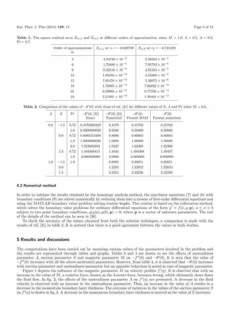
Table 1. The square residual error Em,f and Em,θ at different orders of approximation, when M = 1.0, S = 0.5, A = 0.5,Pr = 0.7.
Order of approximations Em,f at c1 = −0.629739 Em,θ at c2 = −0.741429m
3 4.94720 × 10⁻³ 2.39203 × 10⁻⁴
6 1.70480 × 10⁻⁵ 7.95793 × 10⁻⁶
9 6.22516 × 10⁻⁸ 4.91253 × 10⁻⁷
12 1.85010 × 10⁻¹⁰ 4.55308 × 10⁻⁸
15 7.65476 × 10⁻¹³ 5.39975 × 10⁻⁹
18 1.70985 × 10⁻¹⁵ 7.06892 × 10⁻¹⁰
21 2.29968 × 10⁻¹⁷ 9.77768 × 10⁻¹¹
24 2.21931 × 10⁻¹⁹ 1.38494 × 10⁻¹¹
Table 2. Comparison of the values of −θ′(0) with those of ref. [31] for different values of S, A and Pr when M = 0.0.
A S Pr −θ′(0) [31] −θ′(0) [31] −θ′(0) −θ′(0)Exact Numerical Present HAM Present numerical
0.0 −1.5 0.72 0.4570268328 0.4570 0.45702 0.45702
1.0 0.5000000000 0.5000 0.50000 0.50000
0.0 0.72 0.8086313498 0.8086 0.80863 0.80863
1.0 1.0000000000 1.0000 1.00000 1.00000
3.0 1.923682494 1.9237 1.92368 1.92366
1.5 0.72 1.494368413 1.4944 1.494368 1.49437
1.0 2.000000000 2.0000 2.000000 2.000000
1.0 −1.5 1.0 0.8095 0.80951 0.80951
0.0 1.3205 1.32052 1.32053
1.5 2.2224 2.22236 2.22236
4.2 Numerical method
In order to validate the results obtained by the homotopy analysis method, the non-linear equations (7) and (8) withboundary conditions (9) are solved numerically by reducing them into a system of first-order differential equations andusing the MATLAB boundary value problem solving routine bvp4c. This routine is based on the collocation method,which solves the boundary value problems for ordinary differential equations of the form y′ = f(x, y,p), a ≤ x ≤ bsubject to two point boundary conditions, g(y(a), y(b),p) = 0, where p is a vector of unknown parameters. The restof the details of the method can be seen in [36].
To check the accuracy of the values obtained from both the solution techniques, a comparison is made with theresults of ref. [31] in table 2. It is noticed that there is a good agreement between the values in both studies.
5 Results and discussions
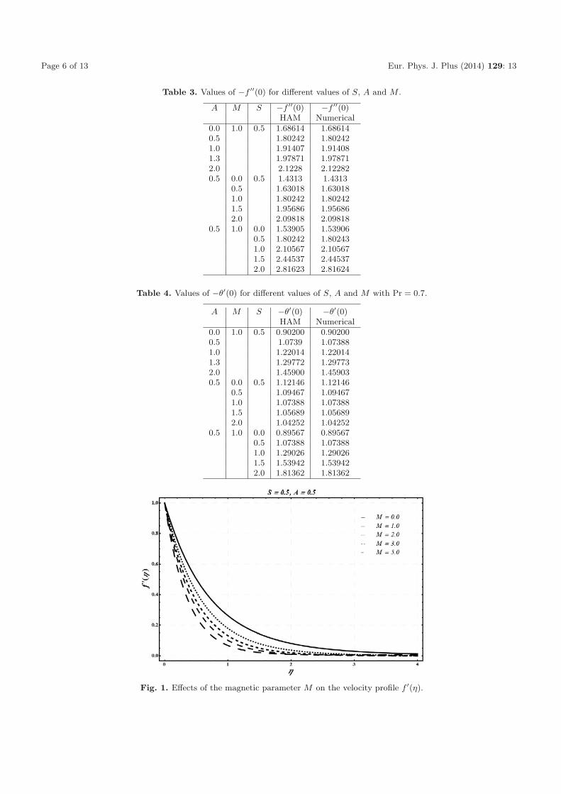
The computations have been carried out by assuming various values of the parameters involved in the problem andthe results are represented through tables and graphs. Tables 3 and 4 are drawn to see the effects of unsteadinessparameter A, suction parameter S and magnetic parameter M on −f ′′(0) and −θ′(0). It is seen that the value of−f ′′(0) increases with all the above-mentioned parameters. However, from table 4, it is observed that −θ′(0) increaseswith suction parameter and unsteadiness parameter but an opposite behaviour is noted in case of magnetic parameter.
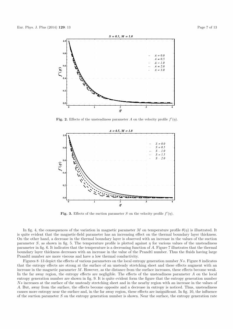
Figure 1 depicts the influence of the magnetic parameter M on velocity profiles f ′(η). It is observed that with anincrease in the value of M , a resistive force, known as the Lorentz force, becomes strong, which ultimately slows downthe fluid flow. In fig. 2, the effects of the unsteadiness parameter A on f ′(η) are presented. A decrease in the fluidvelocity is observed with an increase in the unsteadiness parameter. Thus, an increase in the value of A results in adecrease in the momentum boundary layer thickness. The outcome of variation in the values of the suction parameter Son f ′(η) is shown in fig. 3. A decrease in the momentum boundary layer thickness is noticed as the value of S increases.
Page 6 of 13 Eur. Phys. J. Plus (2014) 129: 13
Table 3. Values of −f ′′(0) for different values of S, A and M .
Fig. 1. Effects of the magnetic parameter M on the velocity profile f ′(η).
Eur. Phys. J. Plus (2014) 129: 13 Page 7 of 13
Fig. 2. Effects of the unsteadiness parameter A on the velocity profile f ′(η).
Fig. 3. Effects of the suction parameter S on the velocity profile f ′(η).
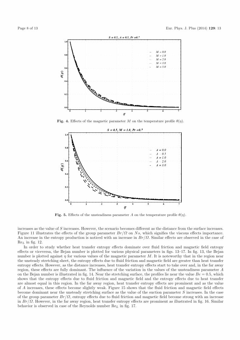
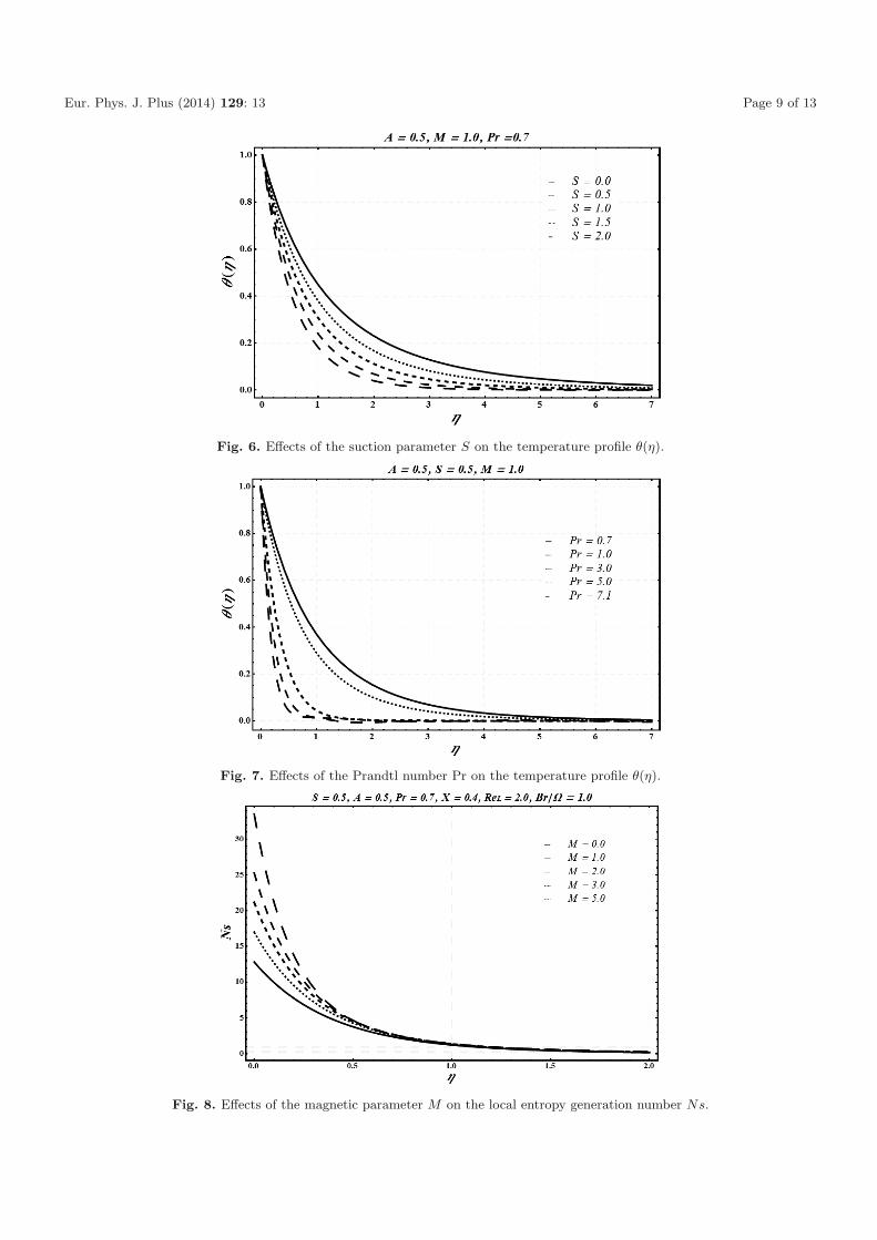
In fig. 4, the consequences of the variation in magnetic parameter M on temperature profile θ(η) is illustrated. Itis quite evident that the magnetic-field parameter has an increasing effect on the thermal boundary layer thickness.On the other hand, a decrease in the thermal boundary layer is observed with an increase in the values of the suctionparameter S, as shown in fig. 5. The temperature profile is plotted against η for various values of the unsteadinessparameter in fig. 6. It indicates that the temperature is a decreasing function of A. Figure 7 illustrates that the thermalboundary layer thickness decreases with an increase in the value of the Prandtl number. Thus the fluids having largePrandtl number are more viscous and have a low thermal conductivity.
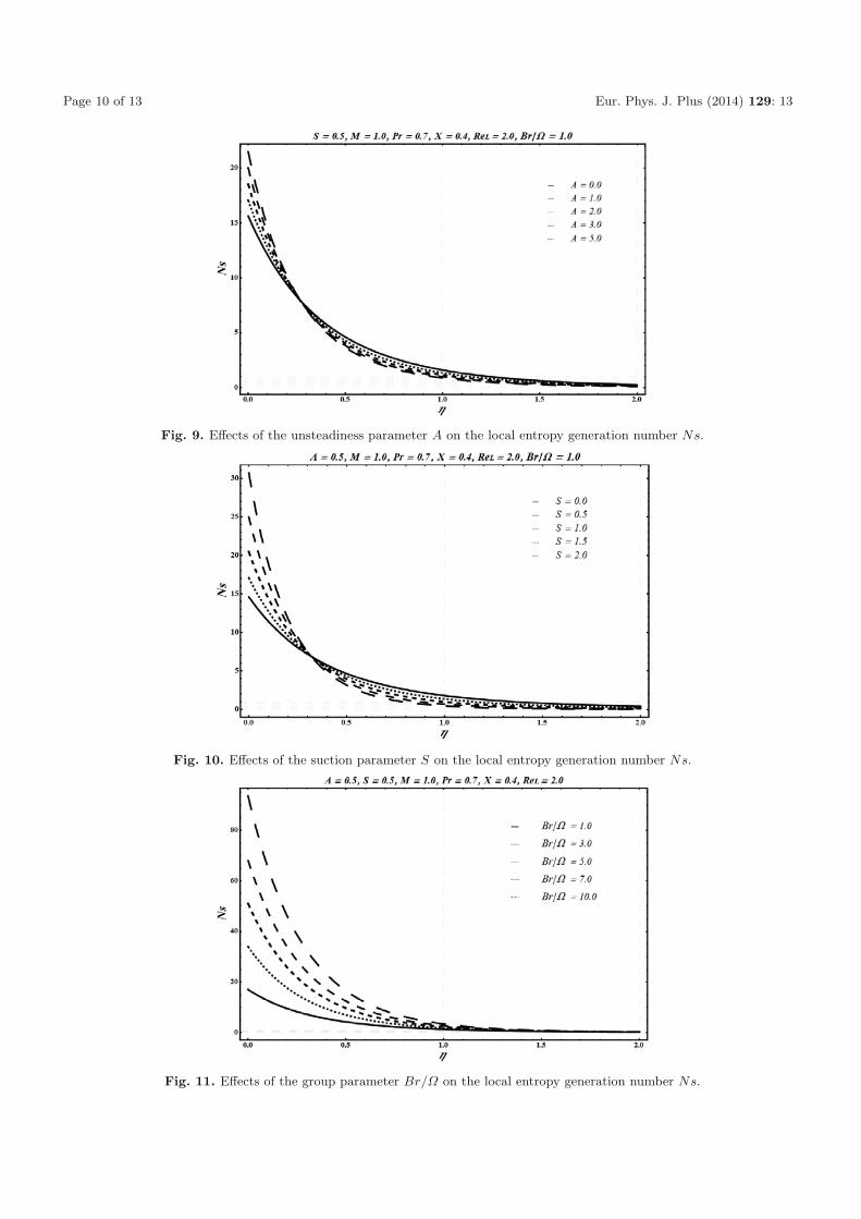
Figures 8–13 depict the effects of various parameters on the local entropy generation number Ns. Figure 8 indicatesthat the entropy effects are strong at the surface of an unsteady stretching sheet and these effects augment with anincrease in the magnetic parameter M . However, as the distance from the surface increases, these effects become weak.In the far away region, the entropy effects are negligible. The effects of the unsteadiness parameter A on the localentropy generation number are shown in fig. 9. It is quite evident form the figure that the entropy generation numberNs increases at the surface of the unsteady stretching sheet and in the nearby region with an increase in the values ofA. But, away from the surface, the effects become opposite and a decrease in entropy is noticed. Thus, unsteadinesscauses more entropy near the surface and, in the far away region, these effects are insignificant. In fig. 10, the influenceof the suction parameter S on the entropy generation number is shown. Near the surface, the entropy generation rate
Page 8 of 13 Eur. Phys. J. Plus (2014) 129: 13
Fig. 4. Effects of the magnetic parameter M on the temperature profile θ(η).
Fig. 5. Effects of the unsteadiness parameter A on the temperature profile θ(η).
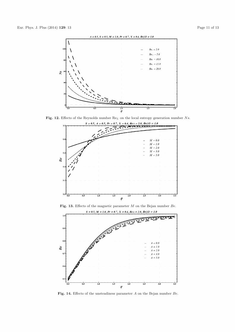
increases as the value of S increases. However, the scenario becomes different as the distance from the surface increases.Figure 11 illustrates the effects of the group parameter Br/Ω on Ns, which signifies the viscous effects importance.An increase in the entropy production is noticed with an increase in Br/Ω. Similar effects are observed in the case ofReL in fig. 12.
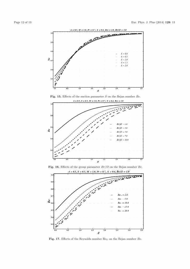
In order to study whether heat transfer entropy effects dominate over fluid friction and magnetic field entropyeffects or viceversa, the Bejan number is plotted for various physical parameters in figs. 13–17. In fig. 13, the Bejannumber is plotted against η for various values of the magnetic parameter M . It is noteworthy that in the region nearthe unsteady stretching sheet, the entropy effects due to fluid friction and magnetic field are greater than heat transferentropy effects. However, as the distance increases, heat transfer entropy effects start to take over and, in the far awayregion, these effects are fully dominant. The influence of the variation in the values of the unsteadiness parameter Aon the Bejan number is illustrated in fig. 14. Near the stretching surface, the profiles lie near the value Be = 0.5, whichshows that the entropy effects due to fluid friction and magnetic field and the entropy effects due to heat transferare almost equal in this region. In the far away region, heat transfer entropy effects are prominent and as the valueof A increases, these effects become slightly weak. Figure 15 shows that the fluid friction and magnetic field effectsbecome dominant near the unsteady stretching surface as the value of the suction parameter S increases. In the caseof the group parameter Br/Ω, entropy effects due to fluid friction and magnetic field become strong with an increasein Br/Ω. However, in the far away region, heat transfer entropy effects are prominent as illustrated in fig. 16. Similarbehavior is observed in case of the Reynolds number ReL in fig. 17.
Eur. Phys. J. Plus (2014) 129: 13 Page 9 of 13
Fig. 6. Effects of the suction parameter S on the temperature profile θ(η).
Fig. 7. Effects of the Prandtl number Pr on the temperature profile θ(η).
Fig. 8. Effects of the magnetic parameter M on the local entropy generation number Ns.
Page 10 of 13 Eur. Phys. J. Plus (2014) 129: 13
Fig. 9. Effects of the unsteadiness parameter A on the local entropy generation number Ns.
Fig. 10. Effects of the suction parameter S on the local entropy generation number Ns.
Fig. 11. Effects of the group parameter Br/Ω on the local entropy generation number Ns.
Eur. Phys. J. Plus (2014) 129: 13 Page 11 of 13
Fig. 12. Effects of the Reynolds number ReL on the local entropy generation number Ns.
Fig. 13. Effects of the magnetic parameter M on the Bejan number Be.
Fig. 14. Effects of the unsteadiness parameter A on the Bejan number Be.
Page 12 of 13 Eur. Phys. J. Plus (2014) 129: 13
Fig. 15. Effects of the suction parameter S on the Bejan number Be.
Fig. 16. Effects of the group parameter Br/Ω on the Bejan number Be.
Fig. 17. Effects of the Reynolds number ReL on the Bejan number Be.
Eur. Phys. J. Plus (2014) 129: 13 Page 13 of 13
6 Conclusions
The entropy effects in boundary layer flow and heat transfer over an unsteady permeable stretching surface, in thepresence of a transverse magnetic field, have been studied. The equations are solved analytically and numerically andthe result are used to investigate the effects of various parameters on velocity, temperature, local entropy generationnumber and Bejan number. The main conclusions drawn from the study are as follows:
– The magnetic field causes the flow to decrease, which results in an increase in the temperature.– The unsteadiness parameter A and the suction parameter S have decreasing effects on velocity and temperature
profiles.– A decrease in the temperature is noticed with an increase in the value of the Prandtl number Pr.– The magnetic parameter M , the group parameter Br/Ω and the Reynolds number ReL augment the entropy
effects which results in an increase in the local entropy generation number Ns.– In the case of suction parameter S and unsteadiness parameter A, Ns increases at the surface and in the neighboring
region with an increase in these parameters. However, the entropy production rate decreases away from the surface.– Near the unsteady stretching surface, the entropy effects due to fluid friction and magnetic field are strong and, in
the far away region, heat transfer entropy effects are in dominance.– The fluid friction and magnetic field entropy effects become strong with an increase in magnetic parameter M ,
suction parameter S, group parameter Br/Ω and Reynolds number ReL near the unsteady stretching surface. Onthe other hand, the entropy effects due to the heat transfer are equal to those of fluid friction and magnetic fieldentropy effects in the case of unsteadiness parameter A.
References
1. A. Bejan, Entropy generation through heat and fluid flow, 2nd edition (Wiley, New York, 1982).2. J.Y. San, Z. Laven, J. Heat Transfer 109, 647 (1987).3. V.S. Arpaci, A. Selamet, J. Thermophys. Heat Transfer 4, 404 (1990).4. S. Mahmud, R.A. Fraser, Int. J. Therm. Sci. 42, 177 (2003).5. M.Q.A. Odat, R.A. Damseh, M.A.A. Nimr, Entropy 4, 293 (2004).6. O.D. Makinde, Phys. Scr. 74, 642 (2006).7. O.D. Makinde, E. Osalusi, Mech. Res. Commun. 33, 692 (2006).8. O.D. Makinde, J. Mech. Sci. Tech. 24, 899 (2010).9. O.D. Makinde, O.A. Beg, J. Therm. Sci. 19, 72 (2010).
10. A. Tamayol, K. Hooman, M. Bahrami, Transp. Porous Med. 85, 661 (2010).11. K. Hooman, A. Ejlali, F. Hooman, Appl. Math. Mech. Engl. Ed. 29, 229 (2008).12. O.D. Makinde, Entropy 13, 1446 (2011).13. O.D. Makinde, Int. J. Exergy 10, 142 (2012).14. A.S. Butt, S. Munawar, A. Ali, A. Mehmood, World Appl. Sci. J. 17, 516 (2012).15. A.S. Butt, S. Munawar, A. Ali, A. Mehmood, Z. Naturforsch. 67a, 451 (2012).16. A.S. Butt, S. Munawar, A. Ali, A. Mehmood, Phys. Scr. 85, 035008 (2012) doi:10.1088/0031-8949/85/03/035008.17. A.S. Butt, S. Munawar, A. Ali, A. Mehmood, J. Mech. Sci. Tech. 26, 2977 (2012).18. A.S. Butt, A. Ali, Chin. Phys. Lett. 30, 024701 (2013).19. S. Munawar, A. Mehmood, A. Ali, Phys. Scr. 86, 065401 (2012).20. L. Crane, Z. Angew. Math. Phys. 21, 645 (1970).21. P.S. Gupta, A.S. Gupta, Can. J. Chem. Eng. 55, 744 (1977).22. J. Grubka, K.M. Bobba, Trans. ASME, J. Heat Transfer 107, 248 (1985).23. T.C. Chiam, Acta Mech. 122, 169 (1997).24. H.S. Takhar, A.J. Chamkha, G. Nath, Int. J. Eng. Sci. 38, 1303 (2000).25. A. Mehmood, A. Ali, ASME J. Heat Transfer 130, 121701 (2008).26. C.Y. Wang, Quart. Appl. Math. 48, 601 (1990).27. H.I. Andersson, J.B. Aarseth, B.S. Dandapat, Int. J. Heat Mass Transfer 43, 69 (2000).28. B.S. Dandapat, B. Santra, H.I. Andersson, Int. J. Heat Mass Transfer 46, 3009 (2003).29. E.M.A. Elbashbeshy, M.A.A. Bazid, Heat Mass Transfer 41, 1 (2004).30. A. Ali, A. Mehmood, Commun. Nonlinear Sci. Numer. Simulat. 13, 340 (2008).31. A. Ishak, R. Nazar, I. Pop, Nonlinear Anal. Real World Appl. 10, 2909 (2010).32. O.D. Makinde, Braz. J. Chem. Eng. 29, 159 (2012).33. S.J. Liao, Beyond perturbation: Introduction to homotopy analysis method (Chapman and Hall, CRC Press, Boca Raton,
2003).34. A. Mehmood, A. Ali, T. Shah, Can. J. Phys. 86, 1079 (2008).35. A. Ali, A. Mehmood, Int. J. Nonlinear Sci. Numer. Simulat. 11, 511 (2010).36. L.F. Shampine, J. Kierzenka, Solving boundary value problems for ordinary differential equations in MATLAB with bvp4c,