A Condensed Form for Nonlinear Differential-Algebraic Equations in Circuit Theory Timo Reis and Tatjana Stykel Abstract We consider nonlinear differential-algebraic equations arising in model- ling of electrical circuits using modified nodal analysis and modified loop analysis. A condensed form for such equations under the action of a constant block diagonal transformation will be derived. This form gives rise to an extraction of over- and underdetermined parts and an index analysis by means of the circuit topology. Fur- thermore, for linear circuits, we construct index-reduced models which preserve the structure of the circuit equations. 1 Introduction One of the most important structural quantities in the theory of differential-algebraic equations (DAEs) is the index. Roughly speaking, the index measures the order of derivatives of the inhomogeneity entering to the solution. Since (numerical) diffe- rentiation is an ill-posed problem, the index can - inter alia - be regarded as a quan- tity that expresses the difficulty in numerical solution of DAEs. In the last three decades various index concepts have been developed in order to characterize dif- ferent properties of DAEs. These are the differentiation index [7], the geometric in- dex [26], the perturbation index [13], the strangeness index [22], and the tractability index [24], to mention only a few. We refer to [25] for a recent survey on all these index concepts and their role in the analysis and numerical treatment of DAEs. In this paper, we present a structure-preserving condensed form for DAEs mo- delling electrical circuits with possibly nonlinear components. This form is inspired Timo Reis Fachbereich Mathematik, Universit¨ at Hamburg, Bundesstraße 55, 22083 Hamburg, Germany, e-mail: [email protected]Tatjana Stykel Institut f¨ ur Mathematik, Universit¨ at Augsburg, Universit¨ atsstraße 14, 86159 Augsburg, Germany, e-mail: [email protected]1
Transcript
A Condensed Form for NonlinearDifferential-Algebraic Equationsin Circuit Theory
Timo Reis and Tatjana Stykel
Abstract We consider nonlinear differential-algebraic equations arising in model-ling of electrical circuits using modified nodal analysis and modified loop analysis.A condensed form for such equations under the action of a constant block diagonaltransformation will be derived. This form gives rise to an extraction of over- andunderdetermined parts and an index analysis by means of the circuit topology. Fur-thermore, for linear circuits, we construct index-reducedmodels which preserve thestructure of the circuit equations.
1 Introduction
One of the most important structural quantities in the theory of differential-algebraicequations (DAEs) is theindex. Roughly speaking, the index measures the order ofderivatives of the inhomogeneity entering to the solution.Since (numerical) diffe-rentiation is an ill-posed problem, the index can - inter alia - be regarded as a quan-tity that expresses the difficulty in numerical solution of DAEs. In the last threedecades various index concepts have been developed in orderto characterize dif-ferent properties of DAEs. These are thedifferentiation index[7], thegeometric in-dex[26], theperturbation index[13], thestrangeness index[22], and thetractabilityindex[24], to mention only a few. We refer to [25] for a recent survey on all theseindex concepts and their role in the analysis and numerical treatment of DAEs.
In this paper, we present a structure-preserving condensedform for DAEs mo-delling electrical circuits with possibly nonlinear components. This form is inspired
by the canonical forms for linear DAEs developed by KUNKEL and MEHRMANN
[17,22]. The latter forms give rise to the so-called strangeness index concept whichhas been successfully applied to the analysis and simulation of structural DAEsfrom different application areas, see the doctoral theses [2, 6, 14, 27, 31–33, 36, 38]supervised by VOLKER MEHRMANN. The great advantage of the strangeness indexis that it can be defined for over- and underdetermined DAEs. Our focus is on circuitDAEs arising frommodified nodal analysis[9, 15, 35] andmodified loop analysis[9, 29]. We show that such DAEs have a very special structure which is preservedin the developed condensed form. In the linear case, we can, furthermore, constructindex-reduced models which also preserve the special structure of circuit equations.
Nomenclature
Throughout this paper, the identity matrix of sizen×n is denoted byIn, or simplyby I if it is clear from context. We writeM > N (M ≥ N) if the square real matrixM −N is symmetric and positive (semi-)definite. The symbol‖x‖ stands for theEuclidean norm ofx ∈ R
n. For a subspaceV ⊂ Rn, V⊥ denotes the orthogonal
complement ofV with respect to the Euclidean inner product. The image and thekernel of a matrixA are denoted by imA and kerA, respectively, and rankA standsfor the rank ofA.
2 Differential-Algebraic Equations
Consider a nonlinear DAE in general form
F(x(t),x(t), t) = 0, (1)
whereF : Dx × Dx × I → Rk is a continuous function,Dx,Dx ⊆ R
n are open,I = [t0, t f ] ⊂ R, x : I → Dx is a continuously differentiable unknown function, and ˙xdenotes the derivative ofx with respect tot.
Definition 2.1. A function x: I → Dx is said to be asolutionof the DAE(1) if itis continuously differentiable for all t∈ I and (1) is fulfilled pointwise for all t∈ I.This function is called asolution of the initial value problem (1)and x(t0) = x0 withx0 ∈ Dx if x is the solution of(1) and satisfies additionally x(t0) = x0. An initialvalue x0 ∈ Dx is calledconsistent, if the initial value problem(1) and x(t0) = x0 hasa solution.
If the functionF has the formF(x,x, t) = x− f (x, t) with f : Dx × I → Rn,
then (1) is an ordinary differential equation (ODE). In thiscase, the assumption ofcontinuity of f gives rise to the consistency of any initial value. If, moreover, f islocally Lipschitz continuous with respect tox then any initial condition determinesthe local solution uniquely [1, Section 7.3].
Let F( ˙x, x, t) = 0 for some( ˙x, x, t) ∈ Dx×Dx× I. If F is partially differentiablewith respect to ˙x and the derivative∂
∂ xF( ˙x, x, t) is an invertible matrix, then by the
A Condensed Form for Nonlinear DAEs in Circuit Theory 3
implicit function theorem [34, Section 17.8] equation (1) can locally be solved forx resulting in an ODE ˙x(t) = f (x(t), t). For general DAEs, however, the solvabilitytheory is much more complex and still not as well understood as for ODEs.
A powerful framework for analysis of DAEs is provided by the derivative arrayapproach introduced in [8]. For the DAE (1) with a sufficiently smooth functionF ,the derivative array of order l∈ N0 is defined by stacking equation (1) and all itsformal derivatives up to orderl , that is,
Fl (x(l+1)(t),x(l)(t), . . . , x(t),x(t), t) =
F(x(t),x(t), t)ddtF(x(t),x(t), t)
...dl
dtlF(x(t),x(t), t)
= 0. (2)
Loosely speaking, the DAE (1) is said to have thedifferentiation indexµd ∈ N0 ifl = µd is the smallest number of differentiations required to determine x from (2)as a function ofx andt. If the differentiation index is well-defined, one can extractfrom the derivative array (2) a so-calledunderlying ODEx(t) = φ(x(t), t) with theproperty that every solution of the DAE (1) also solves the underlying ODE.
Another index concept, calledstrangeness index, was first introduced by KUNKEL
and MEHRMANN for linear DAEs [17, 19, 23] and then extended to the nonlinearcase [20, 22]. The strangeness index is closely related to the differentiation indexand, unlike the latter, can also be defined for over- and underdetermined DAEs [21].For our later proposes, we restrict ourselves to a linear time-varying DAE
E(t)x(t) = A(t)x(t)+ f (t), (3)
whereE ,A : I → Rk,n and f : I → R
k are sufficiently smooth functions. Such a sys-tem can be viewed as a linearization of the nonlinear DAE (1) along a trajectory. Twopairs(E1(t),A1(t)) and(E2(t),A2(t)) of matrix-valued functions are calledgloballyequivalentif there exist a pointwise nonsingular continuous matrix-valued functionU : I → R
k,k and a pointwise nonsingular continuously differentiable matrix-valuedfunctionV : I → R
For (E(t),A(t)) at a fixed pointt ∈ I, the local characteristic valuesr, a ands aredefined as
r = rank(E), a = rank(Z⊤AT), s= rank(S⊤Z⊤AT ′),
where the columns ofZ, T, T ′, andS span kerE⊤, kerE , imE⊤, and kerT⊤A⊤Z,respectively. Considering these values pointwise, we obtain functionsr,a,s: I→N0.It was shown in [17] that under the constant rank conditionsr(t) ≡ r, a(t) ≡ a ands(t) ≡ s, the DAE (3) can be transformed to the globally equivalent system
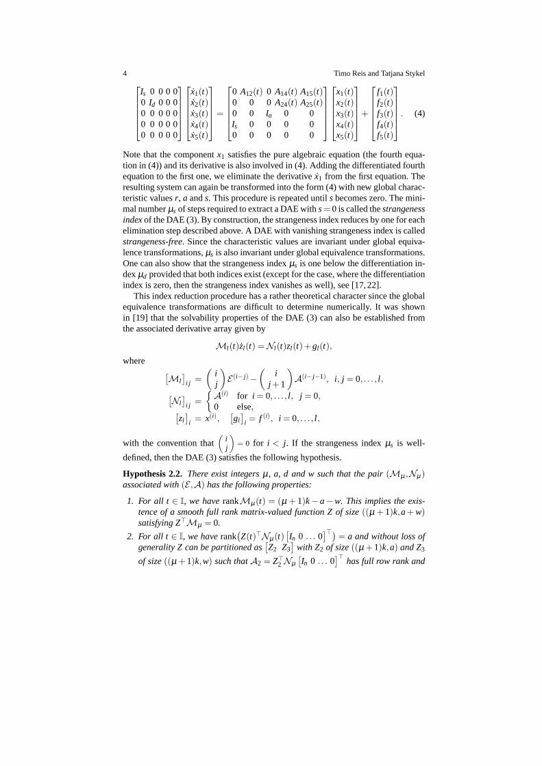
Note that the componentx1 satisfies the pure algebraic equation (the fourth equa-tion in (4)) and its derivative is also involved in (4). Adding the differentiated fourthequation to the first one, we eliminate the derivative ˙x1 from the first equation. Theresulting system can again be transformed into the form (4) with new global charac-teristic valuesr, a ands. This procedure is repeated untilsbecomes zero. The mini-mal numberµs of steps required to extract a DAE withs= 0 is called thestrangenessindexof the DAE (3). By construction, the strangeness index reduces by one for eachelimination step described above. A DAE with vanishing strangeness index is calledstrangeness-free. Since the characteristic values are invariant under global equiva-lence transformations,µs is also invariant under global equivalence transformations.One can also show that the strangeness indexµs is one below the differentiation in-dexµd provided that both indices exist (except for the case, wherethe differentiationindex is zero, then the strangeness index vanishes as well),see [17,22].
This index reduction procedure has a rather theoretical character since the globalequivalence transformations are difficult to determine numerically. It was shownin [19] that the solvability properties of the DAE (3) can also be established fromthe associated derivative array given by
Ml (t)zl (t) = Nl (t)zl (t)+gl (t),
where[Ml
]i j =
(ij
)E (i− j)−
(i
j +1
)A(i− j−1), i, j = 0, . . . , l ,
[Nl
]i j =
{A(i) for i = 0, . . . , l , j = 0,0 else,[
zl]
i = x(i),[gl
]i = f (i), i = 0, . . . , l ,
with the convention that(
ij
)= 0 for i < j. If the strangeness indexµs is well-
defined, then the DAE (3) satisfies the following hypothesis.
Hypothesis 2.2. There exist integersµ , a, d and w such that the pair(Mµ ,Nµ)associated with(E ,A) has the following properties:
1. For all t ∈ I, we haverankMµ(t) = (µ + 1)k− a−w. This implies the exis-tence of a smooth full rank matrix-valued function Z of size((µ + 1)k,a+ w)satisfying Z⊤Mµ = 0.
2. For all t ∈ I, we haverank(Z(t)⊤Nµ(t)
[In 0 . . . 0
]⊤)= a and without loss of
generality Z can be partitioned as[Z2 Z3
]with Z2 of size((µ +1)k,a) and Z3
of size((µ +1)k,w) such thatA2 = Z⊤2 Nµ
[In 0 . . . 0
]⊤has full row rank and
A Condensed Form for Nonlinear DAEs in Circuit Theory 5
Z⊤3 Nµ
[In 0 . . . 0
]⊤= 0. Furthermore, there exists a smooth full rank matrix-
valued function T2 of size(n,n−a) satisfyingA2T2 = 0.3. For all t ∈ I, we haverank
(E(t)T2(t)
)= d, where d= k−a−wµ and
wµ = k− rank[Mµ Nµ
]+ rank
[Mµ−1 Nµ−1
]
with the convention thatrank[M−1 N−1
]= 0. This implies the existence of
a smooth full rank matrix function Z1 of size(k,d) such thatE1 = Z⊤1 E has full
row rank.
The smallest possibleµ in Hypothesis 2.2 is the strangeness index of the DAE(3) andu = n− d− a defines the number of undertermined components. Introdu-cingA1 = Z⊤
1A, f1(t) = Z⊤1 f (t), f2(t) = Z⊤
2 gµ(t) and f3(t) = Z⊤3 gµ(t), we obtain
a strangeness-free DAE systemE1(t)
00
x(t) =
A1(t)A2(t)
0
x(t)+
f1(t)f2(t)f3(t)
(5)
which has the same solutions as (3). The DAE (3) is solvable iff3(t) ≡ 0 in (5).Moreover, an initial conditionx(t0) = x0 is consistent ifA2(t0)x0 + f2(t0) = 0. Theinitial value problem with consistent initial condition has a unique solution ifu= 0.
3 Modified Nodal and Modified Loop Analysis
In this section, we consider the modelling of electrical circuits by DAEs based on theKirchhoff laws and the constitutive relations for the electrical components. Deriva-tions of these relations from Maxwell’s equations can be found in [28].
A general electrical circuit with voltage and current sources, resistors, capacitorsand inductors can be modelled as a directed graph whose nodescorrespond to thenodes of the circuit and whose branches correspond to the circuit elements [9–11,28]. We refer to the aforementioned works for the graph theoretic preliminariesrelated to circuit theory. Letnn, nb andnl be, respectively, the number of nodes,branches and loops in this graph. Moreover, leti(t) ∈ R
nb be the vector of currentsand letv(t)∈R
nb be the vector of corresponding voltages. Then Kirchhoff’s currentlaw [11, 28] states that at any node, the sum of flowing-in currents is equal to thesum of flowing-out currents, see Fig. 1. Equivalently, this law can be written asA0i(t) = 0, whereA0 = [akl ] ∈ R
nn×nb is anall-node incidence matrixwith
akl =
1, if branchl leaves nodek,
−1, if branchl enters nodek,
0, otherwise.
Furthermore, Kirchhoff’s voltage law [11, 28] states that the sum of voltages alongthe branches of any loop vanishes, see Fig. 2. This law can equivalently be writtenasB0v(t) = 0, whereB0 = [bkl ] ∈ R
nl×nb is anall-loop matrixwith
6 Timo Reis and Tatjana Stykel
i1(t)
i2(t)i3(t)
i4(t)
iN(t)
⇒ i1(t)+ . . .+ iN(t) = 0
Fig. 1: Kirchhoff’s current law
v1(t)v2(t)
v3(t)
vN(t)
⇒ v1(t)+ . . .+vN(t) = 0
Fig. 2: Kirchhoff’s voltage law
bkl =
1, if branchl belongs to loopk and has the same orientation,
−1, if branchl belongs to loopk and has the contrary orientation,
0, otherwise.
The following proposition establishes a relation between the incidence and loopmatricesA0 andB0.
Proposition 3.1. [10, p. 213]Let A0 ∈ Rnn×nb be an all-node incidence matrix and
let B0 ∈ Rnl×nb be an all-loop matrix of a connected graph. Then
kerB0 = imA⊤0 , rankA0 = nn−1, rankB0 = nb−nn +1.
We now consider the full rank matricesA∈ Rnn−1×nb andB∈ R
nb−nn+1×nb ob-tained fromA0 andB0, respectively, by removing linear dependent rows. The ma-tricesA andB are called thereduced incidenceandreduced loop matrices, respec-tively. Then the Kirchhoff laws are equivalent to
Ai(t) = 0, Bv(t) = 0. (6)
Due to the relation kerB = imA⊤, we can reformulate Kirchhoff’s laws as follows:there exist vectorsη(t) ∈ R
nn−1 andι(t) ∈ Rnb−nn+1 such that
i(t) = B⊤ι(t), v(t) = A⊤η(t). (7)
The vectorsη(t) andι(t) are called the vectors ofnode potentialsandloop currents,respectively. We partition the voltage and current vectors
A Condensed Form for Nonlinear DAEs in Circuit Theory 7
v(t) =[v⊤C (t) v⊤L (t) v⊤R (t) v⊤
V(t) v⊤I (t)
]⊤,
i(t) =[
i⊤C (t) i⊤L (t) i⊤R (t) i⊤V
(t) i⊤I (t)]⊤
into voltage and current vectors of capacitors, inductors,resistors, voltage and cur-rent sources of dimensionsnC , nL , nR , nV andnI , respectively. Furthermore, parti-tioning the incidence and loop matrices
A =[AC AL AR AV AI
], B =
[BC BL BR BV BI
], (8)
the Kirchhoff laws (6) and (7) can now be represented in two alternative ways,namely, in the incidence-based formulation
AC iC (t)+AL iL(t)+AR iR (t)+AV iV (t)+AI iI(t) = 0, (9)
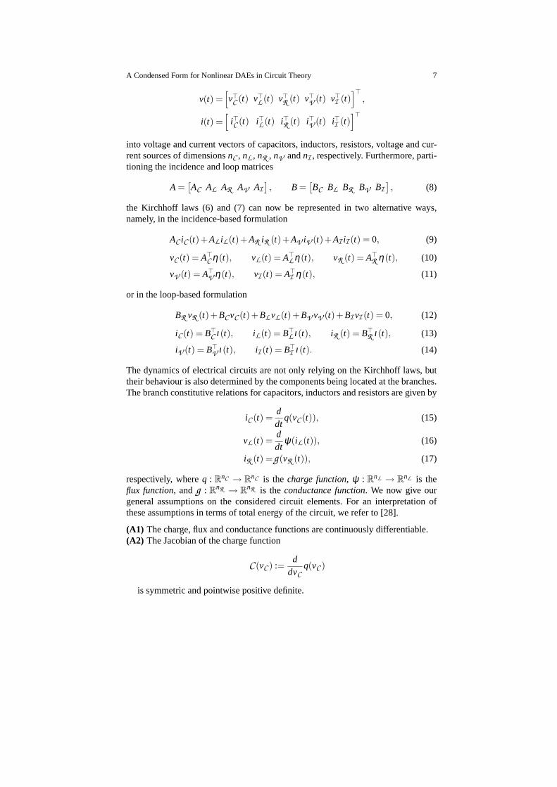
The dynamics of electrical circuits are not only relying on the Kirchhoff laws, buttheir behaviour is also determined by the components being located at the branches.The branch constitutive relations for capacitors, inductors and resistors are given by
iC (t) =ddt
q(vC (t)), (15)
vL(t) =ddt
ψ(iL(t)), (16)
iR (t) =g (vR (t)), (17)
respectively, whereq : RnC → R
nC is thecharge function, ψ : RnL → R
nL is theflux function, andg : R
nR → RnR is theconductance function. We now give our
general assumptions on the considered circuit elements. For an interpretation ofthese assumptions in terms of total energy of the circuit, werefer to [28].
(A1) The charge, flux and conductance functions are continuouslydifferentiable.(A2) The Jacobian of the charge function
C (vC ) :=d
dvCq(vC )
is symmetric and pointwise positive definite.
8 Timo Reis and Tatjana Stykel
(A3) The Jacobian of the flux function
L(iL) :=d
diLψ(iL)
is symmetric and pointwise positive definite.(A4) The conductance function satisfiesg (0) = 0 and there exists a constantc > 0
such that
(vR ,1−vR ,2)⊤(g (vR ,1)−g (vR ,2)
)≥ c‖vR ,1−vR ,2‖
2 (18)
for all vR ,1,vR ,2 ∈ RnR .
Using the chain rule, the relations (15) and (16) can equivalently be written as
iC (t) =C (vC (t))ddt
vC (t), (19)
vL(t) =L(iL(t))ddt
iL(t). (20)
Furthermore, the property (18) implies that the Jacobian ofthe conductance function
G(vR ) :=d
dvRg (vR )
fulfilsG(vR )+G⊤(vR ) ≥ 2cI > 0 for all vR ∈ R
nR . (21)
Thus, the matrixG(vR ) is invertible for all vR ∈ RnR . Applying the Cauchy-
Schwarz inequality to (18) and taking into account thatg (0) = 0, we have
‖g (vR )‖‖vR ‖ ≥ v⊤R g (vR ) ≥ c‖vR ‖2 for all vR ∈ RnR
and, hence,‖g (vR )‖ ≥ cr‖vR ‖. Then it follows from [37, Corollary, p. 201] thatghas a global inverse function. This inverse is denoted byr = g−1 and referred to astheresistance function. Consequently, the relation (17) is equivalent to
vR (t) = r (iR (t)). (22)
Moreover, we obtain from (18) that
(iR ,1− iR ,2
)⊤(r (iR ,1)− r (iR ,2)
)=
(g (r (iR ,1))−g (r (iR ,2))
)⊤(r (iR ,1)− r (iR ,2)
)
=(r (iR ,1)− r (iR ,2)
)⊤(g (r (iR ,1))−g (r (iR ,2))
)≥ c‖r (iR ,1)− r (iR ,2)‖
2
holds for all iR ,1, iR ,2 ∈ RnR . Then the inverse function theorem implies that the
Jacobian
R (iR ) :=d
diRr (iR )
A Condensed Form for Nonlinear DAEs in Circuit Theory 9
fulfils R (iR ) = (G(r (iR )))−1. In particular,R (iR ) is invertible for all iR ∈ RnR ,
and the relation (21) yields
R (iR )+R ⊤(iR ) > 0 for all iR ∈ RnR .
Having collected all physical laws for an electrical circuit, we are now able toset up a circuit model. This can be done in two different ways.The first approachis based on the formulation of Kirchhoff’s laws via the incidence matrices givenin (9)-(11), whereas the second approach relies on the equivalent representation ofKirchhoff’s laws with the loop matrices given in (12)-(14).
a) Modified nodal analysis (MNA)Starting with Kirchhoff’s current law (9), we eliminate theresistive and capaci-tive currents and voltages by using (17) and (19) as well as Kirchhoff’s voltagelaw in (10) for resistors and capacitors. This results in
AC C (A⊤C η(t))A⊤
Cddt η(t)+AR g (A⊤
R η(t))+AL iL(t)+AV iV (t)+AI iI(t) = 0.
Kirchhoff’s voltage law in (10) for the inductive voltages and the componentrelation (20) for the inductors give
−A⊤L η(t)+L(iL(t)) d
dt iL(t) = 0.
Using Kirchhoff’s voltage law in (11) for voltage sources, we obtain finally theMNA system
AC C (A⊤C η(t))A⊤
Cddt η(t)+AR g (A⊤
R η(t))+AL iL(t)+AV iV (t)+AI iI(t)=0,
−A⊤L η(t)+L(iL(t)) d
dt iL(t)=0,
−A⊤V η(t)+vV (t)=0.
(23)In this formulation, voltages of voltage sourcesvV and currents of currentsourcesiI are assumed to be given, whereas node potentialsη , inductive cur-rentsiL and currents of voltage sourcesiV are unknown. The remaining physicalvariables such as voltages of the resistive, capacitive andinductive elements aswell as resistive and capacitive currents can be algebraically reconstructed fromthe solution of system (23).
b) Modified loop analysis (MLA)Using the loop matrix based formulation of Kirchhoff’s voltage law (12), theconstitutive relations (20) and (22) for inductors and resistors, and the loop ma-trix based formulation of Kirchhoff’s current law in (13) for the inductive andresistive currents, we obtain
BL L(B⊤L ι(t))B⊤
Lddt ι(t)+BR r (B⊤
R ι(t))+BC vC (t)+BIvI(t)+BV vV (t) = 0.
Moreover, Kirchhoff’s voltage law in (13) for capacitors together with the com-ponent relation (19) for capacitors gives
10 Timo Reis and Tatjana Stykel
−B⊤C ι(t)+C (vC (t)) d
dt vC (t) = 0.
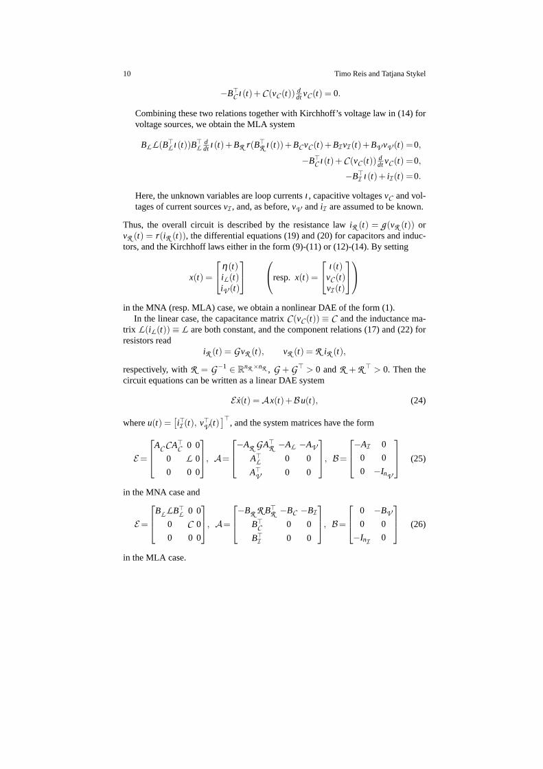
Combining these two relations together with Kirchhoff’s voltage law in (14) forvoltage sources, we obtain the MLA system
BL L(B⊤L ι(t))B⊤
Lddt ι(t)+BR r (B⊤
R ι(t))+BC vC (t)+BIvI(t)+BV vV (t) =0,
−B⊤C ι(t)+C (vC (t)) d
dt vC (t) =0,
−B⊤I ι(t)+ iI(t) =0.
Here, the unknown variables are loop currentsι , capacitive voltagesvC and vol-tages of current sourcesvI , and, as before,vV andiI are assumed to be known.
Thus, the overall circuit is described by the resistance lawiR (t) = g (vR (t)) orvR (t) = r (iR (t)), the differential equations (19) and (20) for capacitors and induc-tors, and the Kirchhoff laws either in the form (9)-(11) or (12)-(14). By setting
x(t) =
η(t)iL(t)iV (t)
resp. x(t) =
ι(t)vC (t)vI(t)
in the MNA (resp. MLA) case, we obtain a nonlinear DAE of the form (1).In the linear case, the capacitance matrixC (vC (t)) ≡ C and the inductance ma-
trix L(iL(t)) ≡ L are both constant, and the component relations (17) and (22)forresistors read
iR (t) = GvR (t), vR (t) = R iR (t),
respectively, withR = G−1 ∈ RnR ×nR , G + G⊤ > 0 andR + R ⊤ > 0. Then the
circuit equations can be written as a linear DAE system
E x(t) = Ax(t)+Bu(t), (24)
whereu(t) =[i⊤I (t), v⊤
V(t)
]⊤, and the system matrices have the form
E=
AC CA⊤C 0 0
0 L 0
0 0 0
, A=
−AR GA⊤
R −AL −AV
A⊤L 0 0
A⊤V
0 0
, B=
−AI 0
0 0
0 −InV
(25)
in the MNA case and
E=
BL LB⊤L 0 0
0 C 0
0 0 0
, A=
−BR R B⊤
R −BC −BI
B⊤C 0 0
B⊤I 0 0
, B=
0 −BV
0 0
−InI 0
(26)
in the MLA case.
A Condensed Form for Nonlinear DAEs in Circuit Theory 11
4 Differential-Algebraic Equations of Circuit Type
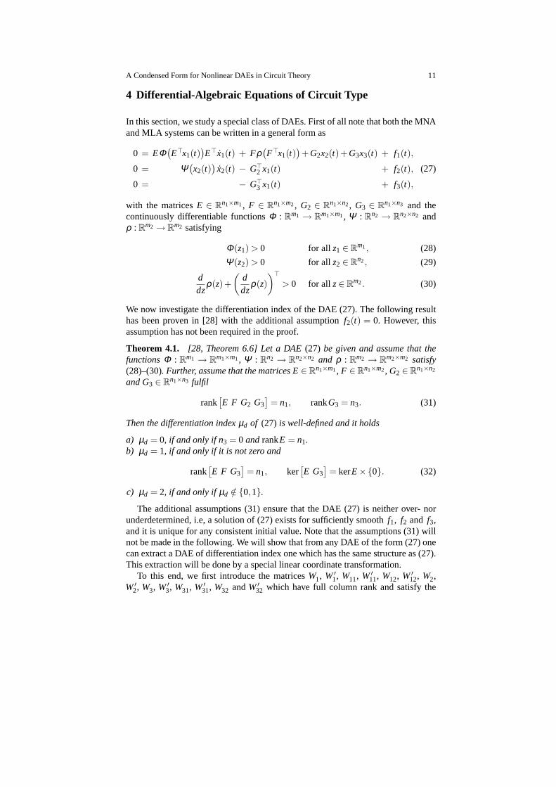
In this section, we study a special class of DAEs. First of allnote that both the MNAand MLA systems can be written in a general form as
0 = EΦ(E⊤x1(t)
)E⊤x1(t) + Fρ
(F⊤x1(t)
)+G2x2(t)+G3x3(t) + f1(t),
0 = Ψ(x2(t)
)x2(t) − G⊤
2 x1(t) + f2(t),
0 = − G⊤3 x1(t) + f3(t),
(27)
with the matricesE ∈ Rn1×m1, F ∈ R
n1×m2, G2 ∈ Rn1×n2, G3 ∈ R
n1×n3 and thecontinuously differentiable functionsΦ : R
m1 → Rm1×m1, Ψ : R
n2 → Rn2×n2 and
ρ : Rm2 → R
m2 satisfying
Φ(z1) > 0 for all z1 ∈ Rm1, (28)
Ψ(z2) > 0 for all z2 ∈ Rn2, (29)
ddz
ρ(z)+
(ddz
ρ(z)
)⊤
> 0 for all z∈ Rm2. (30)
We now investigate the differentiation index of the DAE (27). The following resulthas been proven in [28] with the additional assumptionf2(t) = 0. However, thisassumption has not been required in the proof.
Theorem 4.1. [28, Theorem 6.6] Let a DAE(27) be given and assume that thefunctionsΦ : R
m1 → Rm1×m1, Ψ : R
n2 → Rn2×n2 and ρ : R
m2 → Rm2×m2 satisfy
(28)–(30). Further, assume that the matrices E∈ Rn1×m1, F ∈ R
n1×m2, G2 ∈ Rn1×n2
and G3 ∈ Rn1×n3 fulfil
rank[E F G2 G3
]= n1, rankG3 = n3. (31)
Then the differentiation indexµd of (27) is well-defined and it holds
a) µd = 0, if and only if n3 = 0 andrankE = n1.b) µd = 1, if and only if it is not zero and
rank[E F G3
]= n1, ker
[E G3
]= kerE×{0}. (32)
c) µd = 2, if and only ifµd /∈ {0,1}.
The additional assumptions (31) ensure that the DAE (27) is neither over- norunderdetermined, i.e, a solution of (27) exists for sufficiently smoothf1, f2 and f3,and it is unique for any consistent initial value. Note that the assumptions (31) willnot be made in the following. We will show that from any DAE of the form (27) onecan extract a DAE of differentiation index one which has the same structure as (27).This extraction will be done by a special linear coordinate transformation.
To this end, we first introduce the matricesW1, W′1, W11, W′
11, W12, W′12, W2,
W′2, W3, W′
3, W31, W′31, W32 andW′
32 which have full column rank and satisfy the
12 Timo Reis and Tatjana Stykel
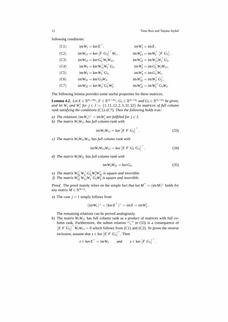
following conditions:
(C1) imW1 = kerE⊤, imW′1 = imE,
(C2) imW11 = ker[F G3
]⊤W1, imW′
11 = imW⊤1
[F G3
],
(C3) imW12 = kerG⊤2 W1W11, imW′
12 = imW⊤11W
⊤1 G2,
(C4) imW2 = kerW⊤11W
⊤1 G2, imW′
2 = imG⊤2 W1W11,
(C5) imW3 = kerW⊤1 G3, imW′
3 = imG⊤3 W1,
(C6) imW31 = kerG3W3, imW′31 = imW⊤
3 G⊤3 ,
(C7) imW32 = kerW⊤3 G⊤
3 W′1, imW′
32 = imW′⊤1 G3W3.
The following lemma provides some useful properties for these matrices.
Lemma 4.2. Let E∈ Rn1×m1, F ∈ R
n1×m2, G2 ∈ Rn1×n2 and G3 ∈ R
n1×n3 be given,and let Wj and W′
j for j ∈ J := {1,11,12,2,3,31,32} be matrices of full columnrank satisfying the conditions(C1)–(C7). Then the following holds true:
a) The relations(imWj)⊥ = imW′
j are fulfilled for j∈ J.b) The matrix W1W11 has full column rank with
imW1W11 = ker[E F G3
]⊤. (33)
c) The matrix W1W11W12 has full column rank with
imW1W11W12 = ker[E F G2 G3
]⊤. (34)
d) The matrix W3W31 has full column rank with
imW3W31 = kerG3. (35)
e) The matrix W′⊤31 W⊤3 G⊤
3 W′1W
′32 is square and invertible.
f) The matrix W′⊤12 W⊤
11W⊤1 G2W′
2 is square and invertible.
Proof. The proof mainly relies on the simple fact that kerM⊤ = (imM)⊥ holds forany matrixM ∈ R
m×n.
a) The casej = 1 simply follows from
(imW1)⊥ = (kerE⊤)⊥ = imE = imW′
1.
The remaining relations can be proved analogously.b) The matrixW1W11 has full column rank as a product of matrices with full co-
lumn rank. Furthermore, the subset relation “⊆” in (33) is a consequence of[E F G3
]⊤W1W11 = 0 which follows from (C1) and (C2). To prove the reverse
inclusion, assume thatx∈ ker[E F G3
]⊤. Then
x∈ kerE⊤ = imW1 and x∈ ker[F G3
]⊤.
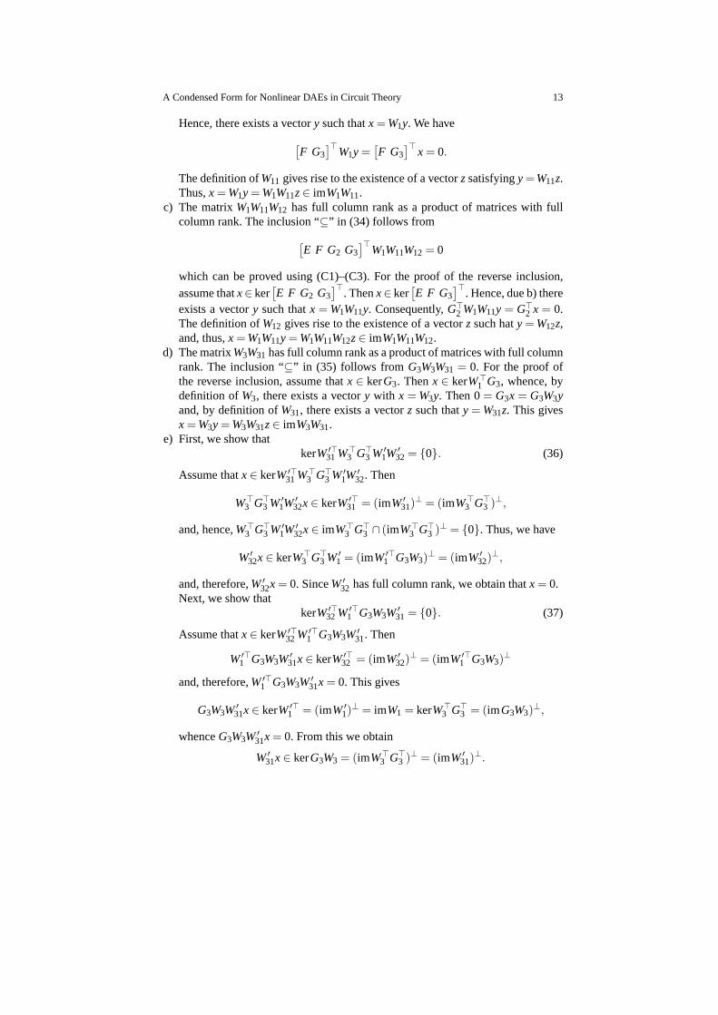
A Condensed Form for Nonlinear DAEs in Circuit Theory 13
Hence, there exists a vectory such thatx = W1y. We have
[F G3
]⊤W1y =
[F G3
]⊤x = 0.
The definition ofW11 gives rise to the existence of a vectorzsatisfyingy=W11z.Thus,x = W1y = W1W11z∈ imW1W11.
c) The matrixW1W11W12 has full column rank as a product of matrices with fullcolumn rank. The inclusion “⊆” in (34) follows from
[E F G2 G3
]⊤W1W11W12 = 0
which can be proved using (C1)–(C3). For the proof of the reverse inclusion,
assume thatx∈ ker[E F G2 G3
]⊤. Thenx∈ ker
[E F G3
]⊤. Hence, due b) there
exists a vectory such thatx = W1W11y. Consequently,G⊤2 W1W11y = G⊤
2 x = 0.The definition ofW12 gives rise to the existence of a vectorz such haty = W12z,and, thus,x = W1W11y = W1W11W12z∈ imW1W11W12.
d) The matrixW3W31 has full column rank as a product of matrices with full columnrank. The inclusion “⊆” in (35) follows from G3W3W31 = 0. For the proof ofthe reverse inclusion, assume thatx ∈ kerG3. Thenx ∈ kerW⊤
1 G3, whence, bydefinition ofW3, there exists a vectory with x = W3y. Then 0= G3x = G3W3yand, by definition ofW31, there exists a vectorz such thaty = W31z. This givesx = W3y = W3W31z∈ imW3W31.
e) First, we show thatkerW′⊤
31 W⊤3 G⊤
3 W′1W
′32 = {0}. (36)
Assume thatx∈ kerW′⊤31 W⊤
3 G⊤3 W′
1W′32. Then
W⊤3 G⊤
3 W′1W
′32x∈ kerW′⊤
31 = (imW′31)
⊥ = (imW⊤3 G⊤
3 )⊥,
and, hence,W⊤3 G⊤
3 W′1W
′32x∈ imW⊤
3 G⊤3 ∩ (imW⊤
3 G⊤3 )⊥ = {0}. Thus, we have
W′32x∈ kerW⊤
3 G⊤3 W′
1 = (imW′⊤1 G3W3)
⊥ = (imW′32)
⊥,
and, therefore,W′32x = 0. SinceW′
32 has full column rank, we obtain thatx = 0.Next, we show that
kerW′⊤32 W′⊤
1 G3W3W′31 = {0}. (37)
Assume thatx∈ kerW′⊤32 W′⊤
1 G3W3W′31. Then
W′⊤1 G3W3W
′31x∈ kerW′⊤
32 = (imW′32)
⊥ = (imW′⊤1 G3W3)
⊥
and, therefore,W′⊤1 G3W3W′
31x = 0. This gives
G3W3W′31x∈ kerW′⊤
1 = (imW′1)
⊥ = imW1 = kerW⊤3 G⊤
3 = (imG3W3)⊥,
whenceG3W3W′31x = 0. From this we obtain
W′31x∈ kerG3W3 = (imW⊤
3 G⊤3 )⊥ = (imW′
31)⊥.
14 Timo Reis and Tatjana Stykel
Thus,W′31x = 0. The property thatW′
31 has full column rank leads tox = 0.Finally, (36) and (37) together imply thatW′⊤
31 W⊤3 G⊤
3 W′1W
′32 is nonsingular.
f) First, we show thatkerW′⊤
12 W⊤11W
⊤1 G2W
′2 = {0}. (38)
Assuming thatx∈ kerW′⊤12 W⊤
11W⊤1 G2W′
2, we have
W⊤11W
⊤1 G2W
′2x∈ kerW′⊤
12 = (imW′12)
⊥ = (imW⊤11W
⊤1 G2)
⊥,
whenceW⊤11W
⊤1 G2W′
2x = 0. This gives rise to
W′2x∈ kerW⊤
11W⊤1 G2 = (imG⊤
2 W1W11)⊥ = (imW′
2)⊥,
and, therefore,W′2x = 0. The fact thatW′
2 has full column rank leads tox = 0.We now show that
kerW′⊤2 G⊤
2 W1W11W′12 = {0}. (39)
Let x∈ kerW′⊤2 G⊤
2 W1W11W′12. Then
G⊤2 W1W11W
′12x∈ kerW′⊤
2 = (imW′2)
⊥ = (imG⊤2 W1W11)
⊥,
and, thus,G⊤2 W1W11W′
12x = 0. Then we have
W′12x∈ kerG⊤
2 W1W11 = (imW⊤11W
⊤1 G2)
⊥ = (imW′12)
⊥,
whenceW′12x = 0. SinceW′
12 has full column rank, we obtain thatx = 0. Finally,it follows from (38) and (39) thatW′⊤
12 W⊤11W
⊤1 G2W′
2 is nonsingular.
⊓⊔
We use the previously introduced matrices and their properties to decompose thevectorsx1(t), x2(t) andx3(t) in the DAE (27) as
x1(t) = W′1W
′32x11(t)+W′
1W32x21(t)+W1W′11x31(t)
+W1W11W′12(W
′⊤2 G⊤
2 W1W11W′12)
−1x41(t)+W1W11W12x51(t),
x2(t) = W′2x12(t)+W2x22(t),
x3(t) = W′3x13(t)+W3W
′31(W
′⊤32 W′⊤
1 G3W3W′31)
−1x23(t)+W3W31x33(t).
(40)
Introducing the vector-valued functions and matrices
x1(t) =
x11(t)
x21(t)
x31(t)
x41(t)
x51(t)
, T1 =
W′⊤32 W′⊤
1
W⊤32W
′⊤1
W′⊤11 W⊤
1
(W′⊤12 W⊤
11W⊤1 G2W′
2)−1W′⊤
12 W⊤11W
⊤1
W⊤12W
⊤11W
⊤1
, (41)
A Condensed Form for Nonlinear DAEs in Circuit Theory 15
x2(t) =
[x12(t)x22(t)
], T2 =
[W′⊤
2
W⊤2
],
x3(t) =
x13(t)x23(t)x33(t)
, T3 =
W′⊤3
(W′⊤31 W⊤
3 G⊤3 W′
1W′32)
−1W′⊤31 W⊤
3
W⊤31W
⊤3
,
(42)
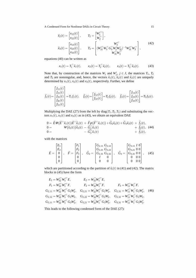
equations (40) can be written as
x1(t) = T⊤1 x1(t), x2(t) = T⊤
2 x2(t), x3(t) = T⊤3 x3(t). (43)
Note that, by construction of the matricesWj andW′j , j ∈ J, the matricesT1, T2
andT3 are nonsingular, and, hence, the vectorsx1(t), x2(t) and x3(t) are uniquelydetermined byx1(t), x2(t) andx3(t), respectively. Further, we define
f1(t)=
f11(t)f21(t)f31(t)f41(t)f51(t)
=T1 f1(t), f2(t)=
[f12(t)f22(t)
]=T2 f2(t), f3(t)=
f13(t)f23(t)f33(t)
=T3 f3(t).
Multiplying the DAE (27) from the left by diag(T1,T2,T3) and substituting the vec-torsx1(t), x2(t) andx3(t) as in (43), we obtain an equivalent DAE
0 = EΦ(E⊤x1(t)
)E⊤ ˙x1(t) + Fρ
(F⊤x1(t)
)+ G2x2(t)+ G3x3(t) + f1(t),
0 = Ψ(x2(t)
) ˙x2(t) − G⊤2 x1(t) + f2(t),
0 = − G⊤3 x1(t) + f3(t),
(44)
with the matrices
E =
E1
E2
000
, F =
F1
F2
F3
00
, G2 =
G2,11 G2,12
G2,21 G2,22
G2,31 G2,32
I 00 0
, G3 =
G3,11 I 0G3,21 0 0G3,31 0 0
0 0 00 0 0
, (45)
which are partitioned according to the partition ofxi(t) in (41) and (42). The matrixblocks in (45) have the form
E1 = W′⊤32 W′⊤
1 E, E2 = W⊤32W
′⊤1 E,
F1 = W′⊤32 W′⊤
1 F, F2 = W⊤32W
′⊤1 F, F3 = W′⊤
11 W⊤1 F,
G2,11 = W′⊤32 W′⊤
1 G2W′2, G2,21 = W⊤
32W′⊤1 G2W
′2, G2,31 = W′⊤
11 W⊤1 G2W
′2,
G2,12 = W′⊤32 W′⊤
1 G2W2, G2,22 = W⊤32W
′⊤1 G2W2, G2,32 = W′⊤
11 W⊤1 G2W2,
G3,11 = W′⊤32 W′⊤
1 G3W′3, G3,21 = W⊤
32W′⊤1 G3W
′3, G3,31 = W′⊤
11 W⊤1 G3W
′3.
(46)
This leads to the following condensed form of the DAE (27):
16T
imo
Reis
andTatjana
Stykel
0
0
0
0
0
0
0
0
0
0
=
E1Φ(E⊤
1 x11(t)+E⊤2 x21(t)
)E⊤
1 x11(t)+E1Φ(E⊤
1 x11(t)+E⊤2 x21(t)
)E⊤
2 x21(t)
E2Φ(E⊤
1 x11(t)+E⊤2 x21(t)
)E⊤
1 x11(t)+E2Φ(E⊤
1 x11(t)+E⊤2 x21(t)
)E⊤
2 x21(t)
0
0
0
W′⊤2 Ψ
(W′
2x12(t)+W2x22(t))W′
2x12(t)+W′⊤2 Ψ
(W′
2x12(t)+W2x22(t))W2x22(t)
W⊤2 Ψ
(W′
2x12(t)+W2x22(t))W′
2x12(t)+W⊤2 Ψ
(W′
2x12(t)+W2x22(t))W2x22(t)
0
0
0
+
F1ρ(F⊤
1 x11(t)+F⊤2 x21(t)+F⊤
3 x31(t))
F2ρ(F⊤
1 x11(t)+F⊤2 x21(t)+F⊤
3 x31(t))
F3ρ(F⊤
1 x11(t)+F⊤2 x21(t)+F⊤
3 x31(t))
0
0
0
0
0
0
0
+
0 0 0 0 0G2,11 G2,12 G3,11 I 0
0 0 0 0 0G2,21 G2,22 G3,21 0 0
0 0 0 0 0G2,31 G2,32 G3,31 0 0
0 0 0 0 0 I 0 0 0 0
0 0 0 0 0 0 0 0 0 0
−G⊤2,11 −G⊤
2,21 −G⊤2,31 −I 0 0 0 0 0 0
−G⊤2,12 −G⊤
2,22 −G⊤2,32 0 0 0 0 0 0 0
−G⊤3,11 −G⊤
3,21 −G⊤3,31 0 0 0 0 0 0 0
−I 0 0 0 0 0 0 0 0 0
0 0 0 0 0 0 0 0 0 0
x11(t)
x21(t)
x31(t)
x41(t)
x51(t)
x12(t)
x22(t)
x13(t)
x23(t)
x33(t)
+
f11(t)
f21(t)
f31(t)
f41(t)
f51(t)
f12(t)
f22(t)
f13(t)
f23(t)
f33(t)
(47)
A Condensed Form for Nonlinear DAEs in Circuit Theory 17
The following facts can be seen from this structure:
a) The componentsx51(t) andx33(t) are actually not involved. As a consequence,they can be chosen freely. It follows from (40) and Lemma 4.2 c) that the vec-tor x51(t) is trivial, i.e., it evolves in the zero-dimensional space,if and only if
ker[E F G2 G3
]⊤= {0}. Furthermore, by Lemma 4.2 d) the vectorx33(t) is
trivial if and only if kerG3 = {0}.b) The componentsf51(t) and f33(t) have to vanish in order to guarantee solvabi-
lity. Due to Lemma 4.2 c), the equationf51(t) = 0 does not appear if and only
if ker[E F G2 G3
]⊤= {0}. Moreover, Lemma 4.2 d) implies that the equation
f33(t) = 0 does not appear if and only if kerG3 = {0}.c) We see from a) and b) that over- and underdetermined parts occur in pairs. This
is a consequence of the symmetric structure of the DAE (27).d) The remaining components fulfil the reduced DAE
0= ErΦ(E⊤
r x1r(t))E⊤
r˙x1r(t) + Frρ
(F⊤
r x1r(t))+ G2r x2r(t)+ G3r x3r(t) + f1r(t),
0= Ψ(x2r(t)
) ˙x2r(t)− G⊤2r x1r(t) + f2r(t),
0= − G⊤3r x1r(t) + f3r(t),
(48)with the matrices, functions and vectors
Er =
E1
E2
00
, Fr =
F1
F2
F3
0
, G2r =
G2,11 G2,12
G2,21 G2,22
G2,31 G2,32
I 0
, G3r =
G3,11 IG3,21 0G3,31 0
0 0
, (49)
x1r(t) =
x11(t)x21(t)x31(t)x41(t)
, f1r(t) =
f11(t)f21(t)f31(t)f41(t)
,
x2r(t) =
[x12(t)x22(t)
]= x2(t), f2r(t) =
[f12(t)f22(t)
]= f2(t),
x3r(t) =
[x13(t)x23(t)
], f3r(t) =
[f13(t)f23(t)
].
(50)
Note that this DAE has the same structure as (27) and (44). It is obtained from(44) by cancelling the componentsx51(t) andx33(t) and the equationsf51(t) = 0and f33(t) = 0.
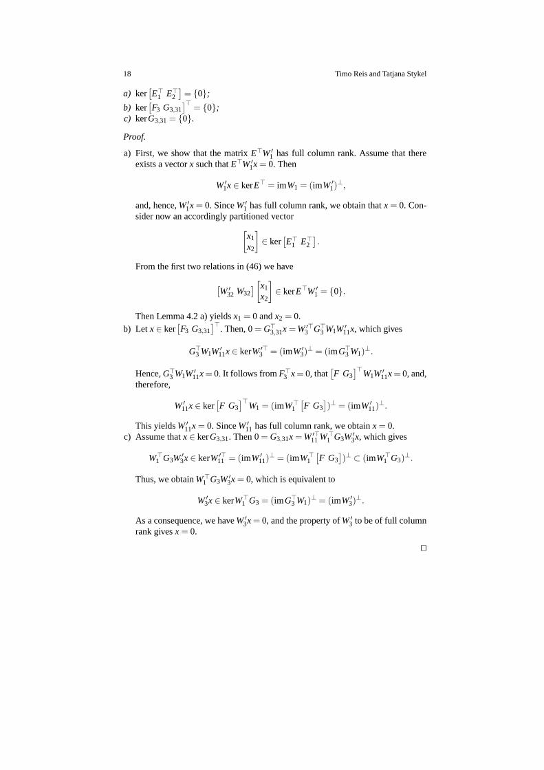
We now analyze the reduced DAE (48). In particular, we show that it satisfies thepreliminaries of Theorem 4.1. For this purpose, we prove thefollowing auxiliaryresult.
Lemma 4.3. Let E∈ Rn1×m1, F ∈ R
n1×m2, G2 ∈ Rn1×n2 and G3 ∈ R
n1×n3 be given.Assume that the matrices Wj and W′
j , j ∈ J, are of full column rank and satisfy theconditions(C1)–(C7). Then for the matrices in(46), the following holds true:
18 Timo Reis and Tatjana Stykel
a) ker[E⊤
1 E⊤2
]= {0};
b) ker[F3 G3,31
]⊤= {0};
c) kerG3,31 = {0}.
Proof.
a) First, we show that the matrixE⊤W′1 has full column rank. Assume that there
exists a vectorx such thatE⊤W′1x = 0. Then
W′1x∈ kerE⊤ = imW1 = (imW′
1)⊥,
and, hence,W′1x = 0. SinceW′
1 has full column rank, we obtain thatx = 0. Con-sider now an accordingly partitioned vector
[x1
x2
]∈ ker
[E⊤
1 E⊤2
].
From the first two relations in (46) we have
[W′
32 W32][
x1
x2
]∈ kerE⊤W′
1 = {0}.
Then Lemma 4.2 a) yieldsx1 = 0 andx2 = 0.
b) Letx∈ ker[F3 G3,31
]⊤. Then, 0= G⊤
3,31x = W′⊤3 G⊤
3 W1W′11x, which gives
G⊤3 W1W
′11x∈ kerW′⊤
3 = (imW′3)
⊥ = (imG⊤3 W1)
⊥.
Hence,G⊤3 W1W′
11x= 0. It follows fromF⊤3 x= 0, that
[F G3
]⊤W1W′
11x= 0, and,therefore,
W′11x∈ ker
[F G3
]⊤W1 = (imW⊤
1
[F G3
])⊥ = (imW′
11)⊥.
This yieldsW′11x = 0. SinceW′
11 has full column rank, we obtainx = 0.c) Assume thatx∈ kerG3,31. Then 0= G3,31x = W′⊤
11 W⊤1 G3W′
3x, which gives
W⊤1 G3W
′3x∈ kerW′⊤
11 = (imW′11)
⊥ = (imW⊤1
[F G3
])⊥ ⊂ (imW⊤
1 G3)⊥.
Thus, we obtainW⊤1 G3W′
3x = 0, which is equivalent to
W′3x∈ kerW⊤
1 G3 = (imG⊤3 W1)
⊥ = (imW′3)
⊥.
As a consequence, we haveW′3x = 0, and the property ofW′
3 to be of full columnrank givesx = 0.
⊓⊔
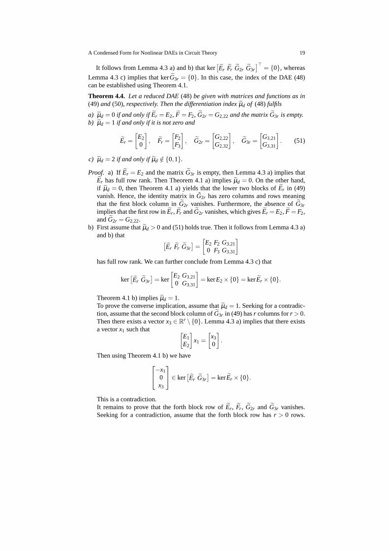
A Condensed Form for Nonlinear DAEs in Circuit Theory 19
It follows from Lemma 4.3 a) and b) that ker[Er Fr G2r G3r
]⊤= {0}, whereas
Lemma 4.3 c) implies that kerG3r = {0}. In this case, the index of the DAE (48)can be established using Theorem 4.1.
Theorem 4.4. Let a reduced DAE(48) be given with matrices and functions as in(49)and (50), respectively. Then the differentiation indexµd of (48) fulfils
a) µd = 0 if and only ifEr = E2, F = F2, G2r = G2,22 and the matrixG3r is empty.b) µd = 1 if and only if it is not zero and
Er =
[E2
0
], Fr =
[F2
F3
], G2r =
[G2,22
G2,32
], G3r =
[G3,21
G3,31
]. (51)
c) µd = 2 if and only if µd /∈ {0,1}.
Proof. a) If Er = E2 and the matrixG3r is empty, then Lemma 4.3 a) implies thatEr has full row rank. Then Theorem 4.1 a) impliesµd = 0. On the other hand,if µd = 0, then Theorem 4.1 a) yields that the lower two blocks ofEr in (49)vanish. Hence, the identity matrix inG2r has zero columns and rows meaningthat the first block column inG2r vanishes. Furthermore, the absence ofG3r
implies that the first row inEr , Fr andG2r vanishes, which givesEr = E2, F = F2,andG2r = G2,22.
b) First assume thatµd > 0 and (51) holds true. Then it follows from Lemma 4.3 a)and b) that
[Er Fr G3r
]=
[E2 F2 G3,21
0 F3 G3,31
]
has full row rank. We can further conclude from Lemma 4.3 c) that
ker[Er G3r
]= ker
[E2 G3,21
0 G3,31
]= kerE2×{0} = kerEr ×{0}.
Theorem 4.1 b) impliesµd = 1.To prove the converse implication, assume thatµd = 1. Seeking for a contradic-tion, assume that the second block column ofG3r in (49) hasr columns forr > 0.Then there exists a vectorx3 ∈ R
r \{0}. Lemma 4.3 a) implies that there existsa vectorx1 such that [
E1
E2
]x1 =
[x3
0
].
Then using Theorem 4.1 b) we have−x1
0x3
∈ ker
[Er G3r
]= kerEr ×{0}.
This is a contradiction.It remains to prove that the forth block row ofEr , Fr , G2r and G3r vanishes.Seeking for a contradiction, assume that the forth block rowhasr > 0 rows.
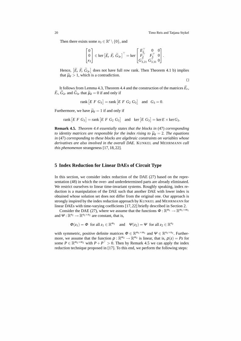
20 Timo Reis and Tatjana Stykel
Then there exists somex3 ∈ Rr \{0}, and
00x3
∈ ker
[Er Fr G3r
]⊤= ker
E⊤2 0 0
F⊤2 F⊤
3 0G⊤
3,21 G⊤3,31 0
.
Hence,[Er Fr G3r
]does not have full row rank. Then Theorem 4.1 b) implies
that µd > 1, which is a contradiction.⊓⊔
It follows from Lemma 4.3, Theorem 4.4 and the construction of the matricesEr ,Fr , G2r andG3r that µd = 0 if and only if
rank[E F G3
]= rank
[E F G2 G3
]and G3 = 0.
Furthermore, we haveµd = 1 if and only if
rank[E F G3
]= rank
[E F G2 G3
]and ker
[E G3
]= kerE×kerG3.
Remark 4.5. Theorem 4.4 essentially states that the blocks in(47) correspondingto identity matrices are responsible for the index rising toµd = 2. The equationsin (47) corresponding to these blocks are algebraic constraints onvariables whosederivatives are also involved in the overall DAE.KUNKEL and MEHRMANN callthis phenomenonstrangeness [17,18,22].
5 Index Reduction for Linear DAEs of Circuit Type
In this section, we consider index reduction of the DAE (27) based on the repre-sentation (48) in which the over- and underdetermined partsare already eliminated.We restrict ourselves to linear time-invariant systems. Roughly speaking, index re-duction is a manipulation of the DAE such that another DAE with lower index isobtained whose solution set does not differ from the original one. Our approach isstrongly inspired by the index reduction approach by KUNKEL and MEHRMANN forlinear DAEs with time-varying coefficients [17,22] briefly described in Section 2.
Consider the DAE (27), where we assume that the functionsΦ : Rm1 → R
m1×m1
andΨ : Rn2 → R
n2×n2 are constant, that is,
Φ(z1) = Φ for all z1 ∈ Rm1 and Ψ(z2) = Ψ for all z2 ∈ R
n2
with symmetric, positive definite matricesΦ ∈ Rm1×m1 andΨ ∈ R
n2×n2. Further-more, we assume that the functionρ : R
m2 → Rm2 is linear, that is,ρ(z) = Pz for
someP ∈ Rm2×m2 with P+ P⊤ > 0. Then by Remark 4.5 we can apply the index
reduction technique proposed in [17]. To this end, we perform the following steps:
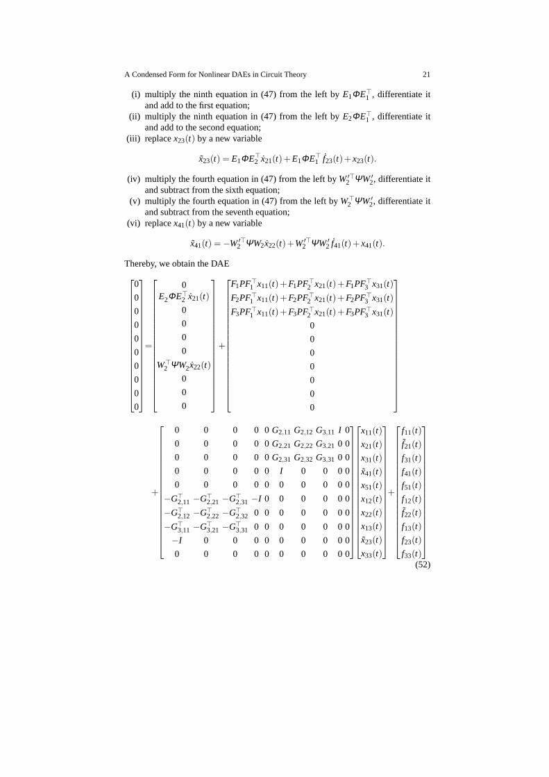
A Condensed Form for Nonlinear DAEs in Circuit Theory 21
(i) multiply the ninth equation in (47) from the left byE1ΦE⊤1 , differentiate it
and add to the first equation;(ii) multiply the ninth equation in (47) from the left byE2ΦE⊤
1 , differentiate itand add to the second equation;
(iii) replacex23(t) by a new variable
x23(t) = E1ΦE⊤2 x21(t)+E1ΦE⊤
1 f23(t)+x23(t).
(iv) multiply the fourth equation in (47) from the left byW′⊤2 ΨW′
2, differentiate itand subtract from the sixth equation;
(v) multiply the fourth equation in (47) from the left byW⊤2 ΨW′
2, differentiate itand subtract from the seventh equation;
(vi) replacex41(t) by a new variable
x41(t) = −W′⊤2 ΨW2x22(t)+W′⊤
2 ΨW′2 f41(t)+x41(t).
Thereby, we obtain the DAE
0
0
0
0
0
0
0
0
0
0
=
0E2ΦE⊤
2 x21(t)
0
0
0
0
W⊤2 ΨW2x22(t)
0
0
0
+
F1PF⊤1 x11(t)+F1PF⊤
2 x21(t)+F1PF⊤3 x31(t)
F2PF⊤1 x11(t)+F2PF⊤
2 x21(t)+F2PF⊤3 x31(t)
F3PF⊤1 x11(t)+F3PF⊤
2 x21(t)+F3PF⊤3 x31(t)
0
0
0
0
0
0
0
+
0 0 0 0 0G2,11 G2,12 G3,11 I 0
0 0 0 0 0G2,21 G2,22 G3,21 0 0
0 0 0 0 0G2,31 G2,32 G3,31 0 0
0 0 0 0 0 I 0 0 0 0
0 0 0 0 0 0 0 0 0 0
−G⊤2,11 −G⊤
2,21 −G⊤2,31 −I 0 0 0 0 0 0
−G⊤2,12 −G⊤
2,22 −G⊤2,32 0 0 0 0 0 0 0
−G⊤3,11 −G⊤
3,21 −G⊤3,31 0 0 0 0 0 0 0
−I 0 0 0 0 0 0 0 0 0
0 0 0 0 0 0 0 0 0 0
x11(t)
x21(t)
x31(t)
x41(t)
x51(t)
x12(t)
x22(t)
x13(t)
x23(t)
x33(t)
+
f11(t)
f21(t)
f31(t)
f41(t)
f51(t)
f12(t)
f22(t)
f13(t)
f23(t)
f33(t)
(52)
22 Timo Reis and Tatjana Stykel
with f21(t) = f21(t)+ E2ΦE⊤1 f23(t) and f22(t) = f22(t)−W⊤
2 ΨW′2 f41(t) which is
again of type (27). Furthermore, it follows from Theorem 4.1and Lemma 4.3 thatthe differentiation index of the resulting DAE obtained from (52) by removing theredundant variablesx51(t) andx33(t) as well as the constrained equations for theinhomogeneity componentsf51(t) = 0 and f33(t) = 0 is at most one.
Remark 5.1.
a) We note that the previously introduced index reduction heavily uses linearity. Inthe case where, for instance,Φ depends on x11(t) and x21(t), the transformation(ii) would be clearly dependent on these variables as well. This causes that theunknown variables x11(t) and x21(t) enter the inhomogeneity f21(t).
b) Structure-preserving index reduction for circuit equations has been consideredpreviously in[3–5]. An index reduction procedure presented there provides a re-duced model which can be interpreted as an electrical circuit containing con-trolled sources. As a consequence, the index-reduced system is not a DAE of type(27)anymore.
6 Consequences for Circuit Equations
In this section, we present a graph-theoretical interpretation of the previous resultsfor circuit equations. First, we collect some basic concepts from the graph theory,which will be used in the subsequent discussion. For more details, we refer to [10].
LetG = (V ,B) be a directed graph with a finite setV of vertices and a finite setB of branches. Forνk1,νk2, an ordered pairbk1 = 〈νk1,νk2〉 denotes a branch leavingνk1 and enteringνk2. A tuple (bk1, . . . ,bks−1) of branchesbk j = 〈νk j ,νk j+1〉 in G iscalled apath connectingνk1 andνks if all verticesνk1, . . . ,νks are different exceptpossiblyνk1 andνks. A path isclosedif νk1 = νks, andopen, otherwise. A closedpath is called aloop. A graphG is calledconnectedif for every two different verticesthere exists an open path connecting them.
A subgraphK = (V ′,B′) of G = (V ,B) is a graph withV ′ ⊆ V andB′ ⊆ B |V ′=
{bk1 = 〈νk1,νk2〉 ∈ B : νk1,νk2 ∈ V ′
}. A subgraphK = (V ′,B′) is
calledspanningif V ′ = V . A spanning subgraphK = (V ,B′) is called acutsetofa connected graphG = (V ,B) if a complementary subgraphG−K = (V ,B \B′)is disconnected andK is minimal with this property. For a spanning subgraphK ofG, a subgraphL of G is called aK-cutset, if L is a cutset ofK. Furthermore, a pathℓ of G is called aK-loop, if ℓ is a loop ofK.
For an electrical circuit, we consider an associated graphG whose vertices cor-respond to the nodes of the circuit and whose branches correspond to the circuitelements. LetA∈R
nn−1×nb andB∈Rnb−nn+1×nb be the reduced incidence and loop
matrices as defined in Section 3. For a spanning graphK of G, we denote byAK
(resp.AG−K) a submatrix ofA formed by the columns corresponding to the branchesin K (resp. the complementary graphG −K). Analogously, we construct the loopmatricesBK andBG−K. By a suitable reordering of the branches, the reduced inci-
A Condensed Form for Nonlinear DAEs in Circuit Theory 23
dence and loop matrices can be partitioned as
A =[AK AG−K
], B =
[BK BG−K
]. (53)
The following lemma from [28] characterizes the absence ofK-loops andK-cutsets in terms of submatrices of the incidence and loop matrices. It is crucialfor our considerations. Note that this result has previously been proven for incidencematrices in [30].
Lemma 6.1 (Subgraphs, incidence and loop matrices [28, Lemma 4.10]). Let Gbe a connected graph with the reduced incidence and loop matrices A∈ R
nn−1×ne
and B∈ Rne−nn+1×ne. Further, letK be a spanning subgraph ofG. Assume that the
branches ofG are sorted in a way that(53) is satisfied.
a) The following three assertions are equivalent:(i) G does not containK-cutsets;
(ii) kerA⊤G−K = {0};
(iii) kerBK = {0}.
b) The following three assertions are equivalent:(i) G does not containK-loops;
(ii) kerAK = {0};(iii) kerB⊤
G−K = {0}.
The next two auxiliary results are concerned with properties of subgraphs ofsubgraphs and give some equivalent characterizations in terms of their incidenceand loop matrices. These statements have first been proven for incidence matricesin [30, Propositions 4.4 and 4.5].
Lemma 6.2(Loops in subgraphs [28, Lemma 4.11]). LetG be a connected graphwith the reduced incidence and loop matrices A∈ R
nn−1×ne and B∈ Rne−nn+1×ne.
Further, letK be a spanning subgraph ofG, and letL be a spanning subgraph ofK. Assume that the branches ofG are sorted in a way that
A =[AL AK−L AG−K
], B =
[BL BK−L BG−K
]. (54)
Then the following three assertions are equivalent:(i) G does not containK-loops except forL-loops;
(ii) For some (and hence any) matrix ZL with imZL = kerA⊤L holds
kerZ⊤LAK−L = {0};
(iii) For some (and hence any) matrix YK−L with imYK−L = kerB⊤K−L holds
Y⊤K−LBG−K = 0.
Lemma 6.3(Cutsets in subgraphs [28, Lemma 4.12]). LetG be a connected graphwith the reduced incidence and loop matrices A∈ R
nn−1×ne and B∈ Rne−nn+1×ne.
24 Timo Reis and Tatjana Stykel
Further, letK be a spanning subgraph ofG, and letL be a spanning subgraph ofK. Assume that the branches ofG are sorted in a way that(54) is satisfied. Then thefollowing three assertions are equivalent:
(i) G does not containK-cutsets except forL-cutsets;(ii) For some (and hence any) matrix YL with imYL = kerB⊤
L holds
kerY⊤L BK−L = {0};
(iii) For some (and hence any) matrix ZK−L with imZK−L = kerA⊤K−L holds
Z⊤K−LAG−K = 0.
We use these results to analyze the condensed form (47) for the MNA equations(23). The MLA equations can be treated analogously. For a given electrical circuitwhose corresponding graph is connected and has no self-loops (see [28]), we intro-duce the following matrices which take the role of the matricesWi andW′
i definedin Section 4. Consider matrices of full column rank satisfying the following condi-tions:
(C1′) imZC = kerA⊤C , imZ′
C = imAC ,
(C2′) imZR V −C = ker[AR AV
]⊤ZC , imZ′
R V −C = imZ⊤C
[AR AV
],
(C3′) imZL−C R V = kerA⊤L ZC ZR V −C , imZ′
L−C R V = imZ⊤R V −C Z⊤
C AL ,
(C4′) im ZL−C R V = kerZ⊤R V −C Z⊤
C AL , im Z′L−C R V = imA⊤
L ZC ZR V −C ,
(C5′) im ZV −C = kerZ⊤C AV , im Z′
V −C = imA⊤V ZC ,
(C6′) im ZV −C = kerAV ZV −C , im Z′V −C = im Z⊤
V −C A⊤V ,
(C7′) im ZC V C = kerZ⊤V −C A⊤
V Z′C , im Z′
C V C = imZ′⊤C AV ZV −C .
Note that the introduced matrices can be determined by computationally cheapgraph search algorithms [12, 16]. We have the following correspondences to thematricesWi andW′
i :
ZC =W1, Z′C =W′
1, ZR V −C =W11, Z′R V −C =W′
11,
ZL−C R V =W12, Z′L−C R V =W′
12, ZL−C R V =W2, Z′L−C R V =W′
2,
ZV −C =W3, Z′V −C =W′
3, ZV −C =W31, Z′V −C =W′
31,
ZC V C =W32, Z′C V C =W′
32.
Using Lemmas 4.2 and 6.1–6.3, we can characterize the absence of certain blocksin the condensed form (47) in terms of the graph structure of the circuit. Based onthe definition ofK-loop andK-cutset, we arrange the following way of speaking.An expression like “C V -loop” indicates a loop in the circuit graph whose branchset consists only of branches corresponding to capacitors and/or voltage sources.
A Condensed Form for Nonlinear DAEs in Circuit Theory 25
Likewise, an “LI-cutset” is a cutset in the circuit graph whose branch set consistsonly of branches corresponding to inductors and/or currentsources.
a) The matrixZC has zero columns if and only if the circuit does not contain anyR LV I-cutsets (Lemma 6.1 a)).
b) The matrixZ′C has zero columns if and only if the circuit does not contain any
capacitors.c) The matrixZR V −C has zero columns if and only if the circuit does not contain
anyLI-cutsets (Lemma 4.2 b) and Lemma 6.1 a)).d) The matrixZ′
R V −Chas zero columns if and only if the circuit does not contain
anyC LI-cutsets except forLI-cutsets (Lemma 6.3).e) The matrixZL−C R V has zero columns if and only if the circuit does not contain
anyI-cutsets (Lemma 4.2 c) and Lemma 6.1 a)).f) The matrixZ′
L−C R V(and by Lemma 4.2 f) also the matrixZ′
L−C R V) has zero
columns if and only if the circuit does not contain anyC R V I-cutsets except forI-cutsets (Lemma 4.2 b) and Lemma 6.3).
g) The matrixZL−C R V has zero columns if and only if the circuit does not containanyR C V L-loops except forR C V -loops (Lemma 4.2 b) and Lemma 6.2)).
h) The matrixZV −C has zero columns if and only if the circuit does not containanyC V -loops except forC -loops (Lemma 6.2).
i) The matrix Z′V −C
has zero columns if and only if the circuit does not containanyR C LI-cutsets except forR LI-cutsets (Lemma 6.3).
j) The matrix ZV −C has zero columns if and only if the circuit does not containanyV -loops (Lemma 4.2 d) and Lemma 6.1 b)).
k) The matrixZ′C V C
(and by Lemma 4.2 e) also the matrixZ′V −C
) has zero columnsif and only if the circuit does not contain anyC V -loops except forC -loops andV -loops (this can be proven analogous to Lemma 6.2).
Exemplarily, we will show a) only. Other assertions can be proved analogously.For the MNA system (23), we haveE = AC . Then by definition, the matrixZC
has zero columns if and only if kerA⊤C = {0}. By Lemma 6.1 a), this condition is
equivalent to the absence ofR LV I-cutsets.In particular, we obtain from the previous findings that the condensed form (47)
does not have any redundant variables and equations if and only if the circuit neithercontainsI-cutsets norV -loops. We can also infer some assertions on the differen-tiation index of the reduced DAE (48) obtained from (47) by removing the redun-dant variables and equations. The DAE (48) has the differentiation indexµd = 0 ifand only if the circuit does not contain voltage sources andR LI-cutsets except forI-cutsets. Furthermore, we haveµd = 1 if and only if and the circuit neither containsC V -loops except forC -loops andV -loops norLI-cutsets except forI-cutsets.
26 Timo Reis and Tatjana Stykel
7 Conclusion
In this paper, we have presented a structural analysis for the MNA and MLA equa-tions which are DAEs modelling electrical circuits with uncontrolled voltage andcurrent sources, resistors, capacitors and inductors. These DAEs are shown to beof the same structure. A special condensed form under lineartransformations hasbeen introduced which allows to determine the differentiation index. In the linearcase, we have presented an index reduction procedure which provides a DAE sys-tem of the differentiation index one and preserves the structure of the circuit DAE.Graph-theoretical characterizations of the condensed form have also been given.
References
1. Arnol’d, V.: Ordinary Differential Equations. Undergraduate Texts in Mathematics. Springer-Verlag, Berlin, Heidelberg, New York (1992). Translated from the Russian by R. Cooke
2. Bachle, S.: Numerical solution of differential-algebraic systems arising in circuit simulation.Ph. D. thesis, Technische Universitat Berlin, Berlin (2007)
3. Bachle, S., Ebert, F.: Element-based index reduction in electrical circuit simulation. In: PAMM- Proc. Appl. Math. Mech., vol. 6, pp. 731–732. Wiley-VCH Verlag GmbH, Weinheim (2006)
4. Bachle, S., Ebert, F.: A structure preserving index reduction method for MNA. In: PAMM -Proc. Appl. Math. Mech., vol. 6, pp. 727–728. Wiley-VCH Verlag GmbH, Weinheim (2006)
5. Bachle, S., Ebert, F.: Index reduction by element-replacementfor electrical circuits. In:G. Ciuprina, D. Ioan (eds.) Scientific Computing in ElectricalEngineering,Mathematics inIndustry, vol. 11, pp. 191–197. Springer-Verlag, Berlin, Heidelberg (2007)
6. Baum, A.K.: A flow-on-manifold formulation of differential-algebraic equations. applicationto positive systems. Ph. D. thesis, Technische Universitat Berlin, Berlin (2014)
7. Brenan, K., Campbell, S., Petzold, L.: The Numerical Solution of Initial-Value Problems inDifferential-Algebraic Equations. Classics in Applied Mathematics, 14. SIAM, Philadelphia,PA (1996)
8. Campbell, S.: A general form for solvable linear time varyingsingular systems of differentialequations. SIAM J. Math. Anal.18(4), 1101–1115 (1987)
9. Chua, L., Desoer, C., Kuh, E.: Linear and Nonlinear Circuits. McGraw-Hill, New York (1987)10. Deo, N.: Graph Theory with Application to Engineering and Computer Science. Prentice-Hall,
Englewood Cliffs, NJ (1974)11. Desoer, C., Kuh, E.: Basic Circuit Theory. McGraw-Hill, New York (1969)12. Estevez Schwarz, D.: A step-by-step approach to compute a consistentinitialization for the
MNA. Int. J. Circuit Theory Appl.30(1), 1–16 (2002)13. Hairer, E., Lubich, C., Roche, M.: The Numerical Solutionof Differential-Algebraic Equa-
tions by Runge-Kutta Methods,Lecture Notes in Mathematics, vol. 1409. Springer-Verlag,Berlin, Heidelberg (1989)
14. Heiland, J.: Decoupling and optimization of differential-algebraic equations with applicationin flow control. Ph. D. thesis, Technische Universitat Berlin, Berlin (2014)
15. Ho, C.W., Ruehli, A., Brennan, P.: The modified nodal approach to network analysis. IEEETrans. Circuits Syst.22(6), 504–509 (1975)
16. Ipach, H.: Graphentheoretische Anwendungen in der Analyse elektrischer Schaltkreise. Bach-elor thesis, Universitat Hamburg, Hamburg, Germany (2013)
17. Kunkel, P., Mehrmann, V.: Canonical forms for linear differential-algebraic equations withvariable coefficients. J. Comput. Appl. Math.56, 225–259 (1994)
18. Kunkel, P., Mehrmann, V.: A new look at pencils of matrix valued functions. Linear AlgebraAppl. 212/213, 215–248 (1994)
A Condensed Form for Nonlinear DAEs in Circuit Theory 27
19. Kunkel, P., Mehrmann, V.: Local and global invariants of linear differential-algebraic equa-tions and their relation. Electron. Trans. Numer. Anal.4, 138–157 (1996)
21. Kunkel, P., Mehrmann, V.: Analysis of over- and underdetermined nonlinear differential-algebraic systems with application to nonlinear control problems. Math. Control Signals Syst.14(3), 233–256 (2001)
23. Kunkel, P., Mehrmann, V., Rath, W.: Analysis and numerical solution of control problems indescriptor form. Math. Control Signals Syst.14(1), 29–61 (2001)
24. Lamour, R., Marz, R., Tischendorf, C.: Differential Algebraic Equations:A Projector BasedAnalysis,Differential-Algebraic Equations Forum, vol. 1. Springer-Verlag, Berlin, Heidelberg(2013)
25. Mehrmann, V.: Index concepts for differential-algebraic equations. Preprint 3-2012, Tech-nische Universitat Berlin (2012). To appear in Encyclopedia of Applied and ComputationalMathematics, Springer-Verlag, Berlin, 2016
26. Rabier, P., Rheinboldt, W.: A geometric treatment of implicit differential-algebraic equations.J. Differential Equations109(1), 110–146 (1994)
27. Rath, W.: Feedback design and regularization for linear descriptor systems with variable co-efficients. Ph. D. thesis, Technische Universitat Chemnitz, Chemnitz (1996)
28. Reis, T.: Mathematical modeling and analysis of nonlinear time-invariant RLC circuits. In:P. Benner, R. Findeisen, D. Flockerzi, U. Reichl, K. Sundmacher (eds.) Large Scale Networksin Engineering and Life Sciences, pp. 126–198. Birkhauser, Basel (2014)
29. Reis, T., Stykel, T.: Lyapunov balancing for passivity-preserving model reduction of RC cir-cuits. SIAM J. Appl. Dyn. Syst.10(1), 1–34 (2011)
30. Riaza, R., Tischendorf, C.: Qualitative features of matrix pencils and DAEs arising in circuitdynamics. Dyn. Syst.22(2), 107–131 (2007)
31. Seufer, I.: Generalized inverses of differential-algebraic equations and their discretization.Ph. D. thesis, Technische Universitat Berlin, Berlin (2005)
32. Shi, C.: Linear differential-algebraic equations of higher-order and the regularity or singularityof matrix polynomials. Ph. D. thesis, Technische Universitat Berlin, Berlin (2004)
33. Steinbrecher, A.: Numerical solution of quasi-linear differential-algebraic equations and in-dustrial simulation of multibody systems. Ph. D. thesis, Technische Universitat Berlin, Berlin(2006)
34. Tao, T.: Analysis II,Texts and Readings in Mathematics, vol. 38. Hindustan Book Agency,New Delhi (2009)
35. Wedepohl, L., Jackson, L.: Modified nodal analysis: an essential addition to electrical circuittheory and analysis. Eng. Science Educ. J.11(3), 84–92 (2002)
36. Weickert, J.: Applications of the theory of differential-algebraic equations to partial differen-tial equations of fluid dynamics. Ph.D. thesis, Technische Universitat Chemnitz, Chemnitz(1997)
37. Wu, F., Desoer, C.: Global inverse function theorem. IEEE Trans. Circuits Syst.19, 199–201(1972)
38. Wunderlich, L.: Analysis and numerical solution of structured and switched differential-algebraic systems. Ph. D. thesis, Technische Universitat Berlin, Berlin (2008)