Journal of Mathematical Psychology 58 (2014) 33–44
Contents lists available at ScienceDirect
Journal of Mathematical Psychology
journal homepage: www.elsevier.com/locate/jmp
A connection between quantum decision theory and quantum games:The Hamiltonian of Strategic Interaction✩
Ismael Martínez-MartínezDüsseldorf Institute for Competition Economics (DICE), Heinrich Heine Universität Düsseldorf, Universitätstraße 1, D-40225 Düsseldorf, Germany
h i g h l i g h t s
• Entanglement between space of actions and beliefs.• Interaction modeled via Hamiltonian based on the theory of quantum angular momentum.• The model has a unique parameter understood as a non-revealed type of the decision-maker.• We obtain a probabilistic analysis of the behavior of the decision-maker.
a r t i c l e i n f o
Article history:Received 23 July 2013Received in revised form20 December 2013
Keywords:RationalityQuantum decision theoryHamiltonian of Strategic InteractionStrategic stateNon-revealed type
a b s t r a c t
Experimental economics and studies in psychology show incompatibilities between human behaviorand the perfect rationality assumption which do not fit in classical decision theory, but a more generalrepresentation in terms of Hilbert spaces can account for them. This paper integrates previous theoreticalworks in quantum game theory, Yukalov and Sornette’s quantum decision theory and Pothos andBusemeyer’s quantum cognition model by postulating the Hamiltonian of Strategic Interaction whichintroduces entanglement in the strategic state of the decision-maker. The Hamiltonian is inherited fromthe algebraic structure of angular momentum in quantum mechanics and the only required parameter,θ ∈ [0, π], represents the strength of the interaction. We consider it as a non-revealed type of thedecision-maker. Considering θ to be a continuous random variable, phenomena like learning whenparticipating in repeated games and the influence of the amount of disposable information could beconsidered as an evolution in the mode and shape of the distribution function fθ (t, I). This modeling ismotivated by the Eisert–Wilkens–Lewenstein quantization scheme for Prisoner’s Dilemmagame and thenit is applied in the Ultimatum game, which is not a simultaneous but a sequential game. Even when thisnon-revealed type θ cannot be directly observed, we can compute observable outcomes: the probabilitiesof offering different amounts of coins and the probability of the different offers being accepted or not bythe other player.
Clearly, much remains to be learnt.May we live in interesting times!
[Ernst Fehr and Antonio Rangel,Journal of Economic Perspectives (2011).]
1. Introduction
There is a growing interest in facing fundamental problemsof economics with tools from other disciplines like computerscience, physics or mathematical psychology. We can find an
✩ I am grateful to Ariane Lambert-Mogiliansky for her fruitful debate and toJerome R. Busemeyer for his precise comments. An early draft of this paper alsobenefited from the discussion with Eric Danan.
increasing number of papers applying concepts from quantummechanics to decision theory problems. Some examples of thisare: a critical revision of decision analysis from the Heisenberg’suncertainty principle by Bordley (1998); a description of the liarparadox considering cognitive acts as quantummeasures by Aerts,Broekaert, and Smets (1999); a general survey on quantumdynam-ics of human decision-making processes and the relevance of theinterference effects by Busemeyer, Wang, and Townsend (2006);the general survey on quantum formalism for cognition (Aerts,Broekaert, & Gabora, 2011), and a conceptual-landscape explana-tion for the Ellsberg paradox by Aerts, D’Hooghe, and Sozzo (2011).
Some aspects of the formulation of quantum decision theoryseem rather simplistic and distant from the economics perspectivein decision theory and the link to game-theoretic reasoning ismissing. Since I consider that we are still far away from havinga formal and definite quantum theory of decision, I adopt thelearning by doing approach in this paper and I want to provide the
34 I. Martínez-Martínez / Journal of Mathematical Psychology 58 (2014) 33–44
reader with a computational technique, instead of entering intomore abstraction.
With this purpose, I propose a general recipe to accountfor deviations from the Nash Equilibrium in games based onpostulating a Hamiltonian of Strategic Interaction (referred asHSI from now on). The seminal idea comes after revising thework of Pothos and Busemeyer (2009) to model human cognitionthrough the Schrödinger’s equation. I find their model to be tooambiguous when defining the parameters ad-hoc, and also non-related to any traditional approach preferred in economics, butthey show how quantum evolution can predict deviations fromrational behavior in decision theory if we are able to implementcognitive dissonances. They apply their model to the Prisoner’sDilemma game interpreting that the player facing the decisionproblem has to consider two subspaces: the subspace of herintention (to play cooperate or defect) and the subspace of whatthe other player is supposed to do (also cooperate or defect). Thecognitive dissonances introduce an entanglement between thesetwo subspaces which leads to a deviation from obtaining only thedominant strategy, defection.
Another way to picture evolution of quantum systems isthrough unitary matrices and, considering that this game of twoplayers and two actions can be understood as two qubits (eachqubit is a quantum two-states system), the Prisoner’s Dilemmaperfectly fits into the formulation of quantum information andquantum computation using qubits and quantum gates to performoperations. This formulation was proposed by Eisert, Wilkens, andLewenstein (1999) (EWL in what follows). The interpretation ofthis paper, concerning how the players can escape the dilemmaby allowing quantum strategies, resulted in a controversy with acomment by Benjamin and Hayden (2001) on the restriction ofthese strategies, but the prescription on how to quantize the Pris-oner’s Dilemma game is not under discussion and it has been afruitful source of inspiration for subsequent papers. Good exam-ples are: Chen, Hogg, and Beausoleil (2003) on how to general-ize to n-player public goods games and the model for quantumCournot’s duopolies under asymmetric information and the studyon how to use entanglement in quantum games to design an eco-nomic regulation for oligopolies by Du, Ju, and Li (2005) and Du,Li, and Ju (2003). From a theoretical point of view, it is also worthto mention the series on quantum game theory applied to marketsby Piotrowski and Sladkowski (2002), Piotrowski, Sladkoski, andSyska (2003), and the proposal for quantum Bayesian implemen-tation byWu (2013), considering failures in traditionalmechanismimplementation inside the quantum domain. Ramzan and Khan(2009) extend the EWL quantization scheme to more than twoplayers, analyzing the effect of communication in a three-playersquantum Prisoner’s Dilemma game. Flitney and Hollenberg (2007)study new Nash equilibria that appear when considering a moregeneral space of strategies and also a multiplayer setting.
These examples are based on the EWL 2 × 2 formulation andits connection with interesting economic problems. In this paper,I want to generalize this formulation to games or situations wherea general number N of strategies is available. Deviation from dom-inant strategy is introduced by the unitary evolution operator thatwe can define from the HSI of the system. The functional formof this Hamiltonian is inherited from the algebraic structure ofangular momenta in quantum mechanics, lying on the geometricproperties of rotations in the space, and hence it is defined by thestructure of available strategies and nothing else. The unitary evo-lution matrix defined in terms of this Hamiltonian plays a simi-lar role to the one performed by the cognitive dissonances (Pothos& Busemeyer) but the HSI model requires only one parameter, θ ,analogous to the parameterγ tuning the entanglement in the EWL-models.
The literature from cognition science recalls the meaning ofthe different parameters in terms of cognitive features and theliterature from quantum information and quantum computationemphasizes the parameters related to entanglement measures. Inthe model by Pothos & Busemeyer, we can see that deviationsfrom perfect rationality arise from the interaction or interferencebetween the space of actions of the decision-maker and her spaceof beliefs, via the Schrödinger time-evolution. In the EWL-modelfor quantum games, the deviations from the classical results arisefrom the interaction between the space of strategies of the twodifferent players, via unitary operations.
I use the mathematical tools of EWL, but considering theinteraction to be between the actions available for a player andher beliefs about the other player, like in the approach by Pothos& Busemeyer. My notation comes from considering the tuningparameter as a non-revealed type of the decision-maker, morerelated to the microeconomic literature. I do not interpret thisfeature in the sense of asymmetric information, but as incompleteinformation. This non-revealed type of the decision-maker isunderstood as ameasure of the strength of the strategic interactionbetween the space of actions and the space of beliefs of thedecision-maker, defined in the HSI. There is a lack of homogeneityin the expressions of ideas in quantumdecisionmodels, so Iwant tostress that applying the evolution defined by the HSI over the basisof the strategic space is away to compute a priori the strategic-stateof the player, given θ .
Section 2 is a brief summary of the basic definitions andconcepts that the reader who is not used to the way of writingin quantum mechanics might find completely new. In order tokeep sense when introducing the new ideas, we strictly followthe survey on the topic developed by Yukalov and Sornette (2008,2009). I present a small summary of their theory, stressing onlyhow to reach the concept of the strategic state of the decision-maker; but the field is broader than this. The reader can alsofind some extra examples of application in Yukalov and Sornette(2011). Other than these, deeper approaches to the paradigm ofrationality inside the non-classical framework are presented in thefinal discussion. Section 3 revisits the EWL formulation for thePrisoner’s Dilemma game showing how the deviation from totaldefection corresponds to the presence of entanglement betweenthe subspaces associated to each player. To illustrate how theEWL solution fits in the HSI general formulation, their notation isslightly modified in Section 4: the model is rewritten to motivatethe jump to the general case of a space of N strategies. Section 5proposes a general prescription for HSI. Prisoner’s Dilemma gameis the simultaneous game par excellence so, in order to show thatthe HSI model can also be applied to sequential games, deviationsfrom the dominant strategy in the discrete Ultimatum game aremodeled in Section 6. Section 7 gathers a discussion on how tointerpret the parameter θ and some final remarks about quantum-like models for decision-making problems.
2. Basics on quantum decision theory
From classical utility formulation to Hilbert spaces
Utility maximization is a key-point when formulating a theoryof decision in classical terms. This approach considers that wecan define a probability measure, dµ(x), over the states of nature,x ∈ X. Besides, every available action, A ∈ A, is assumed to becharacterized by its utility measure, U(A). Under this conditions,we consider the preferred action, A∗, to be such that
A∗∈ argmax
A∈AU(A). (1)
I. Martínez-Martínez / Journal of Mathematical Psychology 58 (2014) 33–44 35
Lack of knowledge on the realization of the different states ofnature introduces uncertainty in the decision problem. Then, theutility of taking an action should be defined as a function of thestate of nature itself,U(A, x). The theory turns into a statistical one,expressed in terms of a joint probability measure, dµ(x, A), whichcan be either continuous or discrete.
Given a probability space for the actions, {A, X, dµ(x, A)}, theexpected utility level of an action A is defined by
U(A) =
X
U(A, x) dµ(x, A). (2)
The joint measure dµ(x, A) is represented in terms of dµ(x) if wecan define
dµ(x, A) = P(A|x) dµ(x), (3)
where P(A|x) is the conditional probability for action A under stateof nature x. Conditional probability notion is useful when we canclassify the elements in the action set A and the elements in theset of nature states X.
Following the classical theory, we are allowed to compare twocompeting actions but we might find difficulties and irregularitiessuch as the impossibility of defining a quantitative measureor taking into account irrational notions such as emotions andsubjective biases, an obstacle tomake amathematical definition ofthe random states of nature, as Yukalov and Sornette discuss. Withthis idea, scale-dependent utility functions U(A) are replaced by anormalized, and then scale-independent, ‘utility’ p(A) such that
p(A) ∈ [0, 1] ∀ A ∈ A, andA∈A
p(A) = 1. (4)
This is a representation of subjective preferences of the decision-maker and also a probability measure itself. Eqs. (2) and (3)govern the selection criterion in classical decision theory,while thequantum decision theory departs from this framework and nowthe most preferred action is associated to the largest probabilityof being selected. In their original discussion Yukalov and Sornette(2008) assume this normalized utility to be
p(A) ≡U(A)
A∈A
U(A). (5)
Since any monotonic transformation of a utility function rep-resents the same preference order, a rigorous interpretation ofdefinition (5) implies a non-desirable range of ambiguity whenmodeling a concrete problem. My intention is to show a way todirectly compute p(A) from the HSI which, as the reader will see inthe following sections, only depends on the preference order andon the realization of the θ value but not on a utility function. Prob-abilities (4) are defined in quantum-mechanical terms, using themathematical theory of separable Hilbert spaces. This proposal re-ceives the name quantum from the analogy with the formalism ofquantummechanics, where unknown hidden variables represent-ing not available quantitative measures are avoided. For the sakeof soundness, using Hilbert spaces to represent the space of statesof the system requires introducing the Dirac’s bra–ket notation1 toexpress the different operations.
1 For simplicity, we just recall that any element or vector of the space of statesis called a ket-vector and represented by the symbol |·⟩. Associated to this, wehave the dual space of the bra-vectors, symbolized by ⟨·|. Given the fact that inthis paper we work only with complex but finite spaces, which are just CN , itis enough for the reader to keep in mind that given a state |ψ⟩ associated to avector ψ ∈ CN , we obtain ⟨ψ | associated to ψĎ , where Ď is the operation ofcomplex conjugation and vector transposition. The name of bra–ket notation comesfrom splitting the bracket⟨·|·⟩ representing the scalar product, which is the crucialoperation to compute probabilities in this framework.
The space of states
A decision-maker faces a variety of intentions and eachintention-representation is a concrete realization of the intention.2Let {|ni⟩} be the representation basis formed by the set of the ba-sic representation states |ni⟩ and exhausting the whole set of in-tentions. The representation basis is orthonormal and the intentionspace,
Hi ≡ L{|ni⟩}, (6)
is the closed linear envelop of the representation basis such thatwehave defined a Hilbert space. The intention state can be expandedin terms of the basis as
|ψ⟩ =
ni
cni |ni⟩. (7)
Intention states are normalized such that
∥ψ∥ = 1, andni
|cni |2
= 1. (8)
A set of several intentions is called a prospect3 and then,a prospect-representation is a concrete implementation of aprospect. The prospect-representation state is the tensor productof the representation states,
|n⟩ =
i
|ni⟩ = |n1n2n3 . . .⟩, (9)
and the prospect-representation basis {|n⟩} is also orthonormal,
⟨m|n⟩ =
i
⟨mi|ni⟩ = δmn =
i
δmini . (10)
Its closed linear envelop defines the prospect-space, which is aHilbert space obtained as the tensor product4 of the intentionspaces,
H = L{|n⟩} =
i
Hi. (11)
For brevity, the prospect-space is usually called mind and its di-mensionality is
dH =
i
Ri, (12)
with Ri the number of representations of the i-intention.
Mind and entanglement
Entanglement is a property of quantum systems presenting atleast two degrees of freedom which are related in such a way thatthe state of some of them cannot be described independently ofthe rest of the system. These systems present a correlation of non-classical nature. We can define:
2 The language adopted by Yukalov and Sornette may seem twisted. For thepurposes of this paper, it is enough for the reader to consider that an intention isnothing but a choice that has to bemade (like what shirt to wear) and the intention-representation is nothing but the available options (like the colors of the shirt).3 Please, do not confuse with the Prospect Theory developed by Kahneman and
Tversky. In the framework by Yukalov and Sornette, the prospect-space is just theset of all feasible combinations among the options in the mind of the decision-maker.4 The tensor product of vector spaces is often called Kronecker product. If further
reading is required, see Chapter II: The mathematical tools of quantum mechanics,Section F: Tensor product of state spaces, pages 153–163 from Cohen-Tannoudji, C.& Bernard Diu, F.L. Quantum Mechanics Volume One, John Wiley & Sons (2005).
36 I. Martínez-Martínez / Journal of Mathematical Psychology 58 (2014) 33–44
• A disentangled prospect-state is a prospect-state that can berepresented as the tensor product of intention states,
|ψ⟩ =
i
|ψi⟩. (13)
Thus, a disentangled mind is the collection of all admissibledisentangled prospect-states, D = {|ψ⟩ : |ψi⟩ ∈ Hi}.
• An entangled prospect-state is any prospect-state, |ψ⟩ ∈ H ,given by
|ψ⟩ =
n
cn|n⟩ andn
|cn|2 = 1, (14)
that cannot be reduced to a tensor product form like (13). Thus,an entangledmind is the complement of the disentangledmindon the product of intention spaces, H \ D .
The decision-making process and the strategic state
Steps in the decision-making process:
1. Evaluation of choices among different actions. The probabilityof realizing a prospect-representation n with the prospect-representation state |n⟩ under a given state-of-mind of theagent ψ is the prospect-probability
pn = |⟨n|ψ⟩|2
= |cn|2
with the normalization conditionn
|cn|2 = 1. (15)
2. The optimal action is the intended action corresponding to themaximal probability.
3. According to the probabilities, a new prospect-representationis selected at the time of making a decision. Decision-makingplus decision-realization forces us to renormalize the stateaccording to the realized action being a certain fact, and hencehaving probability 1 now.
At this point, probabilities (4) can be computed accordingto (15) and it is interesting to recall the interpretation givenby Yukalov and Sornette (2008) to the decision process:
‘‘The decision process corresponding to selecting the maximalprobability supn{pn} is appealing from a behavioral viewpoint, when compared with the expected utility maximizationapproach of normative decision theory’’.
Let us assume that a particular decision-maker is character-ized by a special fixed state in the mind, |s⟩ ∈ H , describingeach decision-maker as a unique subject according to her beliefs,habits... This reference state is called the strategic state. Each mindpossesses a unique strategic state and different decision-makerspossess different strategic states.
Given the strategic state of a decision-maker we can build autility factor for each prospect-representation ψ and we write itp0(ψ). It can play a role analogous to the expected utility in theclassical framework and it is computed in terms of the prospect-representation state |ψ⟩, the prospect-representation basis of themind |n⟩ and the strategic state of the decision-maker, |s⟩:
p0(ψ) =
n
⟨s|PnPψPn|s⟩ =
n
|cn|2⟨s|Pn|s⟩. (16)
Note that the terms of the form ⟨s|Pn|s⟩ play the role of utilities,weighted by the coefficients |cn|2, which are computed from theprojection of the strategic state on the mind basis. The symbols Pnand Pψ represent the projectors |n⟩⟨n| and |ψ⟩⟨ψ |, respectively. Towork with no dependence on the units of measurement, the utilityfactor is normalized soψ∈Ψ
p0(ψ) = 1, (17)
where Ψ represents the total set {|ψ⟩} of all prospect statescorresponding to all admissible prospects, and then forming asubset of the space of mind, which can be called the prospect-stateset Ψ ∈ H .
In an analogous way, after introducing the concept of strategicstate of the decision-maker and the notion of projectors associatedto the prospect-representation states,we candefine the observableprospect-probability for the decision-maker according to
p(ψ) = ⟨s|Pψ |s⟩. (18)
‘‘The concept of an optimal decision is replaced by a probabilis-tic decision, when the prospect, which makes p(ψ) given by(18) maximal, is the one which corresponds best to the givenstrategic state of mind of the decision-maker. In that sense, theprospect that makes p(ψ)maximal can be called optimal withrespect to the strategic state of mind. Using the mapping be-tween the subjective probabilities and the frequentist proba-bilities observed on ensembles of individuals, the prospect thatmakes p(ψ) maximal will be chosen by more individuals thatany other prospect, in the limit of large population samplingsizes. However, other less probable prospects will also be cho-sen by some smaller subset of the population with frequenciesgiven by the corresponding quantum mechanical probabilitiesgiven above’’. (Yukalov & Sornette, 2009)
3. Revising the EWL model for Prisoner’s Dilemma game
The symmetric Prisoner’s Dilemma game is a game involvingtwoplayers,A and B, that can choose among two actions: cooperate(C) or defect (D). Considering the game in its normal form, it isdefined by the canonical payoff matrix
C DC (a, a) (b, d)D (d, b) (c, c)
(19)
where d > a > c > b ensures that mutual cooperation is thePareto optimal situation. Defection is the dominant strategy forboth players, so mutual defection is the Nash equilibrium of thisgame.
Introducing the EWL-model (Eisert et al., 1999), the classicalstrategies available for both players in this game are |C⟩ and |D⟩,that we can assign to the basis of the Hilbert space representing aqubit (which is nothing but a two-state system),
|C⟩ =
10
, |D⟩ =
01
. (20)
We have to consider the mind defined in (11) to be the Hilbertspace given by the tensor product of the spaces associated to PlayerA’s strategy and her evaluation of what Player Bwill choose. Then,H = HA⊗HB is spanned by the basis {|CC⟩, |CD⟩, |DC⟩, |DD⟩} suchthat
|CC⟩ =
1000
, |CD⟩ =
0100
,
|DC⟩ =
0010
, and |DD⟩ =
0001
.(21)
In the proposal by EWL, let the initial state be |ψ0⟩ = |CC⟩.When each player decides whether to play cooperate or defect,the state of the qubit associated to each player should change to
I. Martínez-Martínez / Journal of Mathematical Psychology 58 (2014) 33–44 37
Fig. 1. Left: Standard Prisoner’s Dilemma game represented in terms of qubits andquantum gates. Right: the game with the extra layer S ′ .
picture the decision that has been made. Quantum operations arerepresented by unitary operators and they imply an evolution ofthe state of the system.
We represent strategic moves of Player A and Player B by SA andSB, respectively. According to EWL, the set of quantum strategies isgiven by the 2-parameter set of 2× 2 unitary matrices (see Fig. 1)
U(ξ , φ) =
eiφ cos ξ/2 sin ξ/2− sin ξ/2 e−iφ cos ξ/2
, (22)
with ξ ∈ [0, π] and φ ∈ [0, π/2]. We restrict ourselves to thesubset of classical strategies S0 ≡ {S(ξ) = U(ξ , 0) | ξ ∈ [0, π]}.Cooperate and defect are the two pure strategies
C ≡ S(0) =
1 00 1
and D ≡ S(π) =
0 1
−1 0
. (23)
Hence, the state of the game is given by
|ψ1⟩ = (SA ⊗ SB) |ψ0⟩, (24)
which is a disentangled prospect state of the form (13).From (24)wedirectly see that the onlywayof obtaining PlayerA
not to defect is if this player chooses SA = C , meaning nothing butthat her intention is to cooperate, against the strategic reasoningfor this game. This setup is just the classical Prisoner’s Dilemmagame but represented in terms of a pair of qubits with a coupleof quantum gates acting over them, picturing the choice of theplayers.
Let us now assume that the decision process can be consideredto occur in two different layers: one associated to rational consid-erations (SA ⊗ SB), and another one plotting a spontaneous processwhile taking the decision, S ′. A valid solution to the system pro-posed by EWL is
S ′= exp
iγ
2(D ⊗ D)
, (25)
where γ ∈ [0, π/2] is a real parameter tuning the entanglementof the mind. Explicitly,
S ′=
cos
γ
20 0 i sin
γ
20 cos
γ
2−i sin
γ
20
0 −i sinγ
2cos
γ
20
i sinγ
20 0 cos
γ
2
. (26)
Then,
|ψ2⟩ = S ′(SA ⊗ SB) |ψ0⟩, (27)
which, in the general case, is an entangled prospect state of theform (14). It can only be expressed in the form (13) when γ = 0 orγ = π .
For Player A intending to play defect (this is SA = D), it isstraightforward to compute that the probability (15) of actuallychoosing defect when S ′ is introduced is
PrA(D) = cos2γ
2≤ 1, (28)
so deviations occur in a naturalway for an entangledmind (γ = 0).See Fig. 2.
Example application of the EWL scheme to violations of the Sure ThingPrinciple
In the section above we implicitly assume a four-dimensionalmind of the player. This is so because adopting a game theoreticalpoint of view requires strategic thinking of the players, meaningthat they should reason over their own space of available actionstogether with their foresight over the space of available actionsof the rival. Therefore, the moment when we need to computean observable action of the agent might involve a controversyin terms of how to define a coarse measurement. The mostcommon approach to this problem is not compatible with a coarsemeasurement of only one coordinate in the space of actions of theplayer because of considering the decision to play Defect as a bi-dimensional space spanned by the two coordinates {|DC⟩, |DD⟩}.
A more rigorous approach should focus only on obtaining adecision in the subspace of available actions for Player A, regardlessof what will be the decision of the opponent, and so a differentcoarse measurement in the mind of Player B, even when they aredefined in a symmetric way. Sincewe are dealingwith a composite
Fig. 2. Left: probability of the decision-maker choosing to play defect, given by (28), as a function of the value of the entanglement parameter γ . Right: entropy ofentanglement sAB , given by (34), as a function of the value of the entanglement parameter γ .
38 I. Martínez-Martínez / Journal of Mathematical Psychology 58 (2014) 33–44
system of two subspaces (the space of our own available actions,and the space of opponent’s available actions) we are always ableto get a description of the state of the first subsystemby computingthe partial trace over the second one. The collapse of the mindtowards an observable action would imply a first partial-collapseover the second subsystem B and then the proper measurementover the subsystem A.
As a broad example for this way of computing let us relax fromthe tight example used in Section 3 and let us consider a moregeneral situation in which Player A has to decide whether to defector to cooperate after receiving some information aboutwhat PlayerB will do. This is the problem in Pothos and Busemeyer (2009),where they consider the information about the other player not asa product of a game theoretical reasoning but as an informationalinput for a problem of individual decision-making related to thefindings by Shafir and Tversky (1992) for violations of the SureThing Principle for individual choice under uncertainty.
(i) When Player B is known to Defect we have SB = D and(ii) when Player B is known to Cooperate we have SB = C . (iii)When Player B’s intention is not known, Player A’s perception ofthe situation is the most general case, SB = S(θ) with no extraassumptions on the mixture of strategies. Since Player A’s rationaloutcome should be utility maximizing, SA = D always. Computingfor the general case,
|ψ ′
2⟩ = S ′
D ⊗ S(θ)
|CC⟩ =
i sinγ
2sin
θ
2−i sin
γ
2cos
θ
2cos
γ
2cos
θ
2cos
γ
2sin
θ
2
, (29)
with its associated description in terms of a density matrix ρ givenby
ρ = |ψ ′
2⟩⟨ψ′
2|
=
sin2 γ
2sin2 θ
2−
12sin2 γ
2sin θ
14i sin γ sin θ
12i sin γ sin2 θ
2
−12sin2 γ
2sin θ sin2 γ
2cos2
θ
2−
12i sin γ cos2
θ
2−
14i sin γ sin θ
−14i sin γ sin θ
12i sin γ cos2
θ
2cos2
γ
2cos2
θ
212cos2
γ
2sin θ
−12i sin γ sin2 θ
214i sin γ sin θ
12cos2
γ
2sin θ cos2
γ
2sin2 θ
2
.
(30)
Given the density matrix of the composite system, we obtainthe state of the component A with the operation of partial traceover the subspace of B,
ρA≡ TrBρ. (31)
In this case, we reduce to a 2 × 2 matrix with its matrix elementsdefined as
(ρA)ij =
k∈{C,D}
⟨ik|ρ|jk⟩,
where i, j ∈ {C,D} ⇒ ρA=
sin2 γ
20
0 cos2γ
2
. (32)
Finally, we compute the probability of Player A choosing defectstrategy by introducing the projector PD = |D⟩⟨D|,
PrA(D) = TrρAPD
= cos2
γ
2≤ 1, (33)
in agreement with the result in Eq. (28).
Small deviations from the rational outcomeDefect in thismodelof quantum gates are associated to an increase in the presenceof entanglement in the way that Player A perceives the game asa whole. From (32), the entropy of entanglement between thesubspaces associated to A and B inside the space of the mind isgiven by
sAB = Tr−ρA log ρA
= − cos2γ
2log cos2
γ
2− sin2 γ
2log sin2 γ
2. (34)
In the quantum gates model, releasing information to Player A af-fects the final outcome of the decision if it affects the entanglementin the state of mind of the player. Completely classical players areobtained when γ = 0, corresponding to non-entangled states ofmind and then, recovering the prescription given by Eq. (24). De-viations from the Sure Thing Principle when Player A lacks infor-mation about the state of B is associated to a positive value of theentropy of entanglement of the mind of the player. See Fig. 2. Theobserved departure from pure strategies relates to the presenceof entanglement through the correspondence PrA(D) → γ →
sAB. �
4. Generalization to N strategies
According to game-theoretic reasoning, considering the playersas rational and self-interested agents implies that SA = SB = D forthe Prisoner’s Dilemma game. This translates, in (27), as the oper-ation S ′ acting directly over the tensor product state |DD⟩, whichcorresponds to the tensor product of the two dominant strategies:defect–defect. Concerning S ′, we can rewrite it as follows:
S ′ = expiγ
2(D ⊗ D)
= exp
iγ
2
0 1
−1 0
⊗
0 1
−1 0
= exp
iγ
2(2i)
0 −i2
i2
0
⊗ (2i)
0 −i2
i2
0
= exp−i θ (J2,y ⊗ J2,y)
, (35)
where θ ∈ [0, π], and J2,y is the matrix representing the Jy angularmomentumoperator associated to a two-states system in quantummechanics.
Letting physical considerations aside,5 it is enough to say thatgiven a systemwith total angularmomentum associated to a spaceof states of N components, we can choose the canonical basis
e1 ≡
10...0
, e2 ≡
01...0
, . . . , eN ≡
0...01
∈ CN (36)
to be the eigenstates of the operator Jz . Then, the operator Jy isantisymmetrical and pure imaginary, with its matrix elements
5 Entering into more details about the theory of angular momentum wouldintroduce unnecessary extra complexity in this manuscript, but I stronglyrecommend the reader to consult Chapter VI: General properties of angularmomentum in quantum mechanics and Complement B-VI: Angular momentum androtations, pages 641–676 and 690–711, respectively, from Cohen-Tannoudji, C. &Bernard Diu, F.L. Quantum Mechanics Volume One, John Wiley & Sons (2005).
I. Martínez-Martínez / Journal of Mathematical Psychology 58 (2014) 33–44 39
Fig. 3. Decision-making process for the two agents in a Prisoner’s Dilemma game.There are two different intentions to face: the strategy that each player shouldchoose and the belief about what the other is going to do at the same time.Both intentions have two representations: cooperate or defect. Since the game issimultaneous, δ1 = δ2 = 1 and HSI is built with J2,y for both spaces of strategies.
defined as
(JN,y)m,n
=12i
N − 1
2
N − 1
2+ 1
−
m −
N + 12
m −
N + 12
+ 1δm+1,n
−
N − 1
2
N − 1
2+ 1
−
m −
N + 12
m −
N + 12
− 1δm−1,n
,
(37)
wherem, n ∈ {1, . . . ,N}. The reader can check that definition (37)implies the J2,y matrices in (35), representing the situation in Fig. 3.
5. Postulating the Hamiltonian of Strategic Interaction
S ′ is a unitary operator so it defines an evolution of the quan-tum system that preserves the norm of the state or, in other words,preserves the total probability equal to one. The unitary evolutionoperator giving the state of the system at time t , evolving fromoriginal time t0 = 0, can be expressed in terms of a time-inde-pendent Hamiltonian, say H , according to
U(t, 0) = exp{−iHt}. (38)
From (35), and absorbing the temporal coordinate into the dimen-sionless parameter θ ≡ θ/t , we write
S ′= exp{−iHSI}, (39)
where HSI = θ (J2,y ⊗ J2,y) is the Hamiltonian of Strategic Interac-tion (HSI) associated to theminddescribing the Prisoner’s Dilemmagame.
Now, I propose a general prescription to model the strategicstate |s⟩ of decision-makers facing strategic situations, like games:
1. Let a decision-maker face a problem in which she has todecide for a number K of intentions, labeled by k and each ofthem having Nk possible realizations. Let us also assume thatthe decision-maker is endowed with the ability to establish aranking between the possible realizations.
2. Associated to each intention, there is a Hilbert space, Hk, ofdimension Nk, and spanned by a canonical basis of the form(36). The state |e(k)1 ⟩ represents the best ranked realization forthe intention k, |e(k)2 ⟩ represents the second-best realization forthat intention, and so on.
3. Let |sb⟩ be the strategic state giving, with probability one, thebest realization for every intention,
|sb⟩ =
k
|e(k)1 ⟩. (40)
Because of the choice that we made when defining the basis ofthe space, it will always be the unit vector in the Hilbert spaceof the mind with the first component equal to one and zero inthe rest of them,
|sb⟩ ≡
10...0
∈ CdH , (41)
where dH =
k Nk.4. Identify the information sets in the game, to be able to know
what decisions have to be made at each step of the game. Forexample, the Prisoner’s Dilemma game represents a situationin which both players make a simultaneous choice, but in theexample of the Ultimatum game (that we will illustrate next)the different players make their decisions in a sequential way.
5. The HSI is computed from the angular momentum and theidentity matrices, defined for the different spaces associated tothe intentions to be faced. Decisions that have to be made areaffected by JNk,y and for those that are not, the operator to applyis just the identity matrix INk .
Formally, we can define the Hamiltonian of StrategicInteraction in the most general case as
HSI = θ
Kk=1
δkJNk,y + (1 − δk) INk
, (42)
where δk is just an indicator function such that δk = 1 if theintention k has to be decided at the step of the game that weare considering or δk = 0 if not.
6. The strategic state of the decision-maker is then
|s⟩ = S ′|sb⟩, (43)
where S ′ is defined by (39) and (42), and the prospect probabil-ities can be computed according to (15).
(*) When the game is sequential, the state of the mind should beupdated after each decision has been made. As usual in quan-tum mechanics, the state after the measurement is directlygiven by the eigenstate associated to the outcome that is ob-served and, therefore, it is always a pure state until some newevolution takes place.
6. Example of application: the Ultimatum game
In the Ultimatum game, a total amount ofmoney is given to twoplayers and then, the first player chooses to make an offer on howto split themoney. PlayerB can accept (A) or refuse (R). If this playeraccepts, they get the money split according to the offer but, if thisplayer refuses, both players get zero. Let us consider the case forN = 10 coins. The dominant strategy for Player B is to accept anynon-zero amount of coins, while the dominant strategy for Player Ais to offer a non-zero amount of money as close to zero as possible,n = 1 in this case.
Computing the strategic states
Let us model now the decision process of Player A. She has twointentions to face: (i) howmany coins to offer and (ii) howdoes she
40 I. Martínez-Martínez / Journal of Mathematical Psychology 58 (2014) 33–44
Fig. 4. Decision-making process for the Player A in the Ultimatum game. In theexample, up to N = 10 coins are the strategic offers that Player A can propose.When making a decision, Player A expects Player B to accept (A) after she releasesher proposal. In this case, the game is sequential, so δ1 = 1 and δ2 = 0 and HSI isbuilt with J10,y and I2 .
expect Player B to react to her offer. Intention 1 has ten differentrepresentations: from giving n = 1 coins to n = 10 coins. See Fig. 4(and compare to 3, corresponding to the PD previously studied). Anatural monotonic ordering for the actions is
n = 1 ≻ n = 2 ≻ · · · ≻ n = 10, (44)
allowing us to associate θ to the departure from standard perfectrationality in a positive way. This also defines the ordering of theelements of the basis in the Hilbert space of the first intention,H1 = C10. For the second intention, A ≻ R, and we have definedthe basis in H2 = C2. Hence, the strategic state |sb⟩ (41) is
|sb⟩ =
10...0
∈ C20. (45)
According to the fact that this game is sequential, the HSI (42)is just
HSI = θ (J10,y ⊗ I2), (46)
where
J10,y
=
0 −3i2
0 0 0 0 0 0 0 03i2
0 −2i 0 0 0 0 0 0 0
0 2i 0 −i√212
0 0 0 0 0 0
0 0i√212
0 −i√6 0 0 0 0 0
0 0 0 i√6 0 −
5i2
0 0 0 0
0 0 0 05i2
0 −i√6 0 0 0
0 0 0 0 0 i√6 0 −
i√212
0 0
0 0 0 0 0 0i√212
0 −2i 0
0 0 0 0 0 0 0 2i 0 −3i2
0 0 0 0 0 0 0 03i2
0
and I2 =
1 00 1
. (47)
S ′ given by (39) can be easily computed using any computa-tional software with an algebraic package. Finally, applying S ′ over|sb⟩ we get the strategic state of Player A, in terms of θ , given by
|s⟩ = S ′|sb⟩ =
cos(θ/2)9
03 cos(θ/2)8 sin(θ/2)
0364
cosec(θ/2)5 sin θ7
0√2132
cosec(θ/2)3 sin θ6
0316
72cosec(θ/2) sin θ5
038
72sin(θ/2) sin θ4
0√214
sin(θ/2)3 sin θ3
032sin(θ/2)5 sin θ2
032sin(θ/2)7 sin θ
0sin(θ/2)9
0
. (48)
Then, the strategic state of the Player A is a superposition ofstates weighted in the following way,
cos
θ
2
9
|1A⟩ + 3 cos
θ
2
8
sin
θ
2
|2A⟩ + · · ·
+ sin
θ
2
9
|10A⟩. (49)
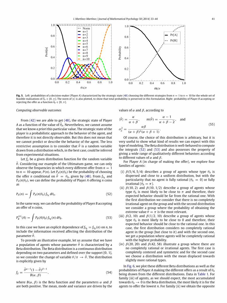
Given the value of θ , the decision-maker will choose tooffer n = 1 coin expecting Player B to accept with probabilitycos(θ/2)9
2, and so on with the other terms. We can see how the
probabilities for the different offers are determined as a functionof the parameter θ in Fig. 5. Since this is the setup for Player A, letθ = θA. The probability of offering an amount of coins bigger thanone is non-vanishing, unless θA = 0.
Once the decision about the offer has been made, the state ofthe game collapses to the subspace associated to the offer that hasbeen made, and then Player B has to decide whether to accept orrefuse. In this case, and for Player B,
HSI = θ (I10 ⊗ J2,y), (50)
where I10 is the 10 × 10 identity matrix, and J2y =
0 −
i2
i2
0
.
We get the final strategic state for Player B given by
cosθ
2|nA⟩ + sin
θ
2|nR⟩,
for the different realizations of the offer n. (51)Recall that the strategic state of Player B belongs to a different mind,so θ ≡ θB in (51). The probability of accepting is cos2 θB/2 < 1,unless θB = 0. See Fig. 5.
I. Martínez-Martínez / Journal of Mathematical Psychology 58 (2014) 33–44 41
Fig. 5. Left: probabilities of a decision-maker (Player A) characterized by the strategic state (48) choosing the different strategies from n = 1 to n = 10 for the whole set offeasible realizations of θA ∈ [0, π]. The norm of |s⟩ is also plotted, to show that total probability is preserved in this formulation. Right: probability of Player B accepting orrejecting the offer as a function θB ∈ [0, π].
Computing observable outcomes
From (42) we are able to get (48), the strategic state of PlayerA as a function of the value of θA. Nevertheless, we cannot assumethatwe know a priori this particular value. The strategic state of theplayer is a probabilistic approach to the behavior of the agent, andtherefore it is not directly observable. But this does not mean thatwe cannot predict or describe the behavior of the agent. The lessrestrictive assumption is to consider that θ is a random variabledrawn from a distributionwhich, in the best case, could be inferredfrom experimental situations.
Let fθ be a given distribution function for the random variableθ . Considering our example of the Ultimatum game, we can onlyobserve the frequencies in which every different offer from n = 1to n = 10 appear, P(n). Let PA(n|θA) be the probability of choosingthe offer n conditional on θ = θA, given by (48). From fθA andPA(n|θA), we can define the probability of Player A offering n coinsas
PA(n) =
PA(n|θA) fθA dθA. (52)
In the sameway,we candefine the probability of Player B acceptingan offer of n coins,
P (n)B (A) =
PB(A|θB) fθB(n) dθB. (53)
In this case we have an explicit dependence of fθB = fθB(n) on n, toinclude the information received affecting the distribution of theparameter θ .
To provide an illustrative example, let us assume that we havea population of agents whose parameter θ is characterized by aBeta distribution. The Beta distribution is a continuous distributiondepending on two parameters and defined over the support [0, 1],so we consider the change of variable θ/π → θ . The distributionis explicitly given by
fθ =θα−1(1 − θ )β−1
B(α, β), (54)
where B(α, β) is the Beta function and the parameters α and βare both positive. The mean, mode and variance are driven by the
values of α and β , according to
⟨θ⟩ =α
α + β, m(θ) =
α − 1α + β − 2
, and
σ 2θ
=αβ
(α + β)2(α + β + 1).
(55)
Of course, the choice of this distribution is arbitrary, but it isvery useful to show what kind of results we can expect with thistype ofmodeling. The Beta distribution iswell-behaved to computethe integrals (52) and (53) and also possesses the property ofgiving a wide range of qualitatively different behaviors accordingto different values of α and β .
For Player A (in charge of making the offer), we explore fourfamilies of agents:
(i) β(5/4, 5/4) describes a group of agents whose type θA isdispersed and close to a uniform distribution, but with theparticularity that no agent is fully rational (θA = 0) or fullyirrational (θA = π ).
(ii) β(10, 2) and β(10, 1/2) describe a group of agents whosetype θA is most likely to be close to π and therefore, theirexpected behavior should be far from the rational one. Withthe first distribution we consider that there is no completelyirrational agent on the group andwith the second distributionwe consider a group where the probability of obtaining theextreme value θ = π is the most relevant.
(iii) β(2, 10) and β(1/2, 10) describe a group of agents whosetype θA is most likely to be close to 0 and therefore, theirexpected behavior should be close to the rational one. In thiscase, the first distribution considers no completely rationalagent in the group (but close to it) and with the second one,we get a population where agents will be completely rationalwith the highest probability.
(iv) β(20, 20) and β(42, 58) illustrate a group where there areno completely rational or irrational agents. The first case iscompletely centered and symmetric and for the second casewe choose a distribution with the mean displaced towardsslightly more rational types.
In Fig. 6, we plot these different Beta distributions as well as theprobabilities of Player Amaking the different offers as a result of θAbeing drawn from the different distributions. Data in Table 1. Forfamily (iii) of agents, as we should expect, the most accumulatedtowards θA → 0 is the Beta distribution, themost likely it is for theagents to offer the lowest n. For family (ii) we obtain the opposite
42 I. Martínez-Martínez / Journal of Mathematical Psychology 58 (2014) 33–44
Table 1Numerical value for PA(n; α, β), the probabilities (52) of Player A offering the different amounts of coins, as a function of the parameters α and β , governing the distributionof θA . They are plotted in Fig. 6. (*) Columns might not exactly add up to 1 due to rounding to four decimal places in the table.
Fig. 6. (1) Top left: different Beta distributions for Player A’s type representing the four different qualitative behaviors. (2) Probability of Player A offering the differentamounts of coins, n, for: top right—family (ii) of agents, bottom left—family (iii) of agents, and bottom right—families (i) and (iv) of agents. Numerical values in Table 1.
case. For family (i) we get an almost uniform probability for thedifferent offers and, finally, for family (iv) we get the interestingbehavior of agents making fair offers. For the completely symmet-ricβ(20, 20)weget the peak on offering 5 or 6 coins. Forβ(42, 58),we obtain themaximumprobability for the case of offering 4 coins.This kind of fair offers are very often observed. See the meta-analysis performed byOosterbeek, Sloof, and Van de Kuilen (2004).
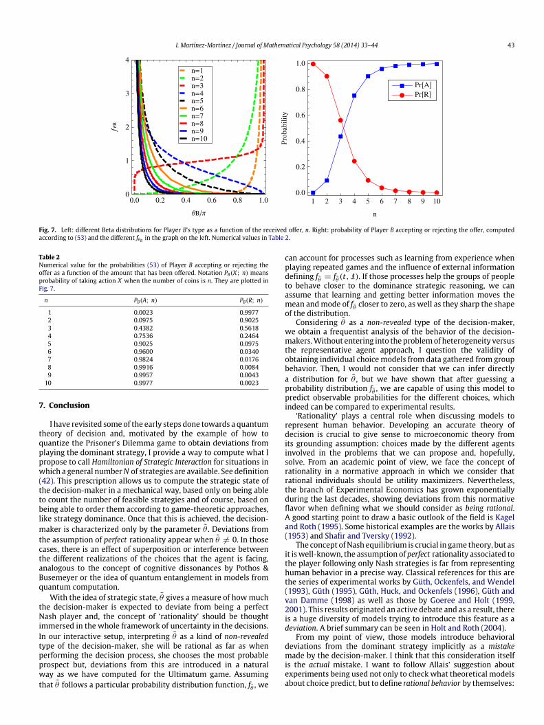
Let us now describe how population B will react. Consideringagain agents described by their random variable θB drawn from aBeta distribution, we have to take into account the fact that theoffer receivedmight affect the distribution. Sincewe are just tryingto provide an example of how to compute refutable outcomes forthis model, there is no harm in considering the distribution to befθB = β(N/n2, n2/N) where N = 10 is the maximum number of
coins that can be offered and n is the offer that has been received.With this choice we have a population whose mean and mode offθB will move closer to zero the bigger the offer. In this way, thewillingness to accept an offer increases with the amount of coins,which seems quite natural. See Fig. 7.
We get relevant probability (>75%) of accepting the offer whenit is 4 coins or more. Experiments in games use different setups:sometimes the intention to accept or reject the different offersshould be announced in a strategic way, before a particular offerhas been received, but sometimes it should be decided only afterthe offer is released. Then, since experimental data on receiver’sbehavior are less concluding than studies for the proposer, seeagain Oosterbeek et al. (2004), we just consider this modeling asa computational example.
I. Martínez-Martínez / Journal of Mathematical Psychology 58 (2014) 33–44 43
Fig. 7. Left: different Beta distributions for Player B’s type as a function of the received offer, n. Right: probability of Player B accepting or rejecting the offer, computedaccording to (53) and the different fθB in the graph on the left. Numerical values in Table 2.
Table 2Numerical value for the probabilities (53) of Player B accepting or rejecting theoffer as a function of the amount that has been offered. Notation PB(X; n) meansprobability of taking action X when the number of coins is n. They are plotted inFig. 7.
I have revisited some of the early steps done towards a quantumtheory of decision and, motivated by the example of how toquantize the Prisoner’s Dilemma game to obtain deviations fromplaying the dominant strategy, I provide a way to compute what Ipropose to call Hamiltonian of Strategic Interaction for situations inwhich a general numberN of strategies are available. See definition(42). This prescription allows us to compute the strategic state ofthe decision-maker in a mechanical way, based only on being ableto count the number of feasible strategies and of course, based onbeing able to order them according to game-theoretic approaches,like strategy dominance. Once that this is achieved, the decision-maker is characterized only by the parameter θ . Deviations fromthe assumption of perfect rationality appear when θ = 0. In thosecases, there is an effect of superposition or interference betweenthe different realizations of the choices that the agent is facing,analogous to the concept of cognitive dissonances by Pothos &Busemeyer or the idea of quantum entanglement in models fromquantum computation.
With the idea of strategic state, θ gives a measure of howmuchthe decision-maker is expected to deviate from being a perfectNash player and, the concept of ‘rationality’ should be thoughtimmersed in the whole framework of uncertainty in the decisions.In our interactive setup, interpreting θ as a kind of non-revealedtype of the decision-maker, she will be rational as far as whenperforming the decision process, she chooses the most probableprospect but, deviations from this are introduced in a naturalway as we have computed for the Ultimatum game. Assumingthat θ follows a particular probability distribution function, fθ , we
can account for processes such as learning from experience whenplaying repeated games and the influence of external informationdefining fθ = fθ (t, I). If those processes help the groups of peopleto behave closer to the dominance strategic reasoning, we canassume that learning and getting better information moves themean andmode of fθ closer to zero, as well as they sharp the shapeof the distribution.
Considering θ as a non-revealed type of the decision-maker,we obtain a frequentist analysis of the behavior of the decision-makers.Without entering into the problemof heterogeneity versusthe representative agent approach, I question the validity ofobtaining individual choicemodels from data gathered from groupbehavior. Then, I would not consider that we can infer directlya distribution for θ , but we have shown that after guessing aprobability distribution fθ , we are capable of using this model topredict observable probabilities for the different choices, whichindeed can be compared to experimental results.
‘Rationality’ plays a central role when discussing models torepresent human behavior. Developing an accurate theory ofdecision is crucial to give sense to microeconomic theory fromits grounding assumption: choices made by the different agentsinvolved in the problems that we can propose and, hopefully,solve. From an academic point of view, we face the concept ofrationality in a normative approach in which we consider thatrational individuals should be utility maximizers. Nevertheless,the branch of Experimental Economics has grown exponentiallyduring the last decades, showing deviations from this normativeflavor when defining what we should consider as being rational.A good starting point to draw a basic outlook of the field is Kageland Roth (1995). Some historical examples are the works by Allais(1953) and Shafir and Tversky (1992).
The concept ofNash equilibrium is crucial in game theory, but asit iswell-known, the assumption of perfect rationality associated tothe player following only Nash strategies is far from representinghuman behavior in a precise way. Classical references for this arethe series of experimental works by Güth, Ockenfels, and Wendel(1993), Güth (1995), Güth, Huck, and Ockenfels (1996), Güth andvan Damme (1998) as well as those by Goeree and Holt (1999,2001). This results originated an active debate and as a result, thereis a huge diversity of models trying to introduce this feature as adeviation. A brief summary can be seen in Holt and Roth (2004).
From my point of view, those models introduce behavioraldeviations from the dominant strategy implicitly as a mistakemade by the decision-maker. I think that this consideration itselfis the actual mistake. I want to follow Allais’ suggestion aboutexperiments being used not only to check what theoretical modelsabout choice predict, but to define rational behavior by themselves:
44 I. Martínez-Martínez / Journal of Mathematical Psychology 58 (2014) 33–44
‘‘Rationality can [also] be defined experimentally by observingthe actions of peoplewho can be regarded as acting in a rationalmanner’’. (Allais, 1953)
I find really interesting the discussion by Fehr and Rangel(2011) about the necessity for Economics to step aside from thenormative concept of rationality and the convenience to movetowards a behavioral definition of this. There is no structuralmodel for behavioral economics already available, but the debatetowards a new paradigm of rationality is thrilling. We can seea good compendium of some of the work that has been donein Diamond and Vartiainen (2007). From Eq. (5), the reader mightconsider an analogy between the framework adopted in thispaper and the solution concept for games called Quantal ResponseEquilibrium (McKelvey & Palfrey, 1995). This does not hold ingeneral for the non-classical approach to decision problems andwe can find more elaborated and fundamental works in the fieldof non-classical decision theory that should be considered in theframework of bounded rationality. Individuals characterized bypreferences are interpreted as measurable systems by Danilov andLambert-Mogiliansky (2008). This approach was later axiomatizedtowards a theory of expected utility (Danilov & Lambert-Mogiliansky, 2010). It is also worth to mention the model forthe Kahneman–Tversky man where preferences are determined(not just revealed) in the process of measurement by Lambert-Mogiliansky, Zamir, and Zwirn (2009) as well as the model forself-control in dynamic context where type indeterminacy impliesthe decision-maker to split in different selves facing the problems,by Lambert-Mogiliansky and Busemeyer (2012).
References
Aerts, D., Broekaert, J., & Gabora, L. (2011). A case for applying an abstractedquantum formalism to cognition. New ideas in Psychology, 29, 136–146.
Aerts, D., Broekaert, J., & Smets, S. (1999). A quantum structure description of theliar paradox. International Journal of Theoeretical Physics, 38, 3231–3239.
Aerts, D., D’Hooghe, B., & Sozzo, S. (2011). A quantum cognition analysis of theEllsberg paradox. In Quantum interaction: 5th international symposium, QI 2011,Aberdeen, UK, June 26–29, 2011, Revised selected papers. Berlin, Heidelberg:Springer.
Allais, M. (1953). Le comportement de l’homme rationnel devant le risque: Critiquedes postulats et axiomes de l’école americaine. Econometrica, 21, 503–546.
Benjamin, S. C., & Hayden, P. M. (2001). Comment on quantum games and quantumstrategies. Physical Review Letters, 87.
Bordley, R. F. (1998). Quantum mechanical and human violations of compoundprobability principles: toward a generalized Heisenberg uncertainty principle.Operations Research, 46, 923–926.
Busemeyer, J. R., Wang, Z., & Townsend, J. T. (2006). Quantum dynamics of humandecision-making. Journal of Mathematical Psychology, 50, 220–241.
Chen, K. Y., Hogg, T., & Beausoleil, R. (2003). A quantum treatment of public goodseconomics. Quantum Information Processing , 1, 449–469.
Danilov, V. I., & Lambert-Mogiliansky, A. (2008). Measurable systems andbehavioral sciences.Mathematical Social Sciences, 55, 315–340.
Danilov, V. I., & Lambert-Mogiliansky, A. (2010). Expected utility theory under non-classical uncertainty. Theory and Decision, 68, 25–47.
Diamond, P. A., & Vartiainen, H. e. (2007). Behavioral economics and its applications.Princeton University Press.
Du, J., Ju, C., & Li, H. (2005). Quantum entanglement helps in improving economicefficiency. Journal of Physics A: Mathematical and General, 38, 1559–1565.
Du, J., Li, H., & Ju, C. (2003). Quantum games of asymmetric information. PhysicalReview E, 68.
Eisert, J., Wilkens, M., & Lewenstein, M. (1999). Quantum games and quantumstrategies. Physical Review Letters, 83, 3077–3080.
Fehr, E., & Rangel, A. (2011). Neuroeconomic foundations of economic choice —Recent advances. Journal of Economic Perspectives, 25, 3–30.
Flitney, A. P., & Hollenberg, L. C. (2007). Nash equilibria on quantum games withgeneralized two-parameter strategies. Physics Letters A, 363, 381–388.
Goeree, J. K., & Holt, C. A. (1999). Stochastic game theory: for playing games, notjust for doing theory. PNAS, 96, 10564–10567.
Goeree, J. K., & Holt, C. A. (2001). Ten little treasures of game theory and thenintuitive contradictions. The American Economic Review, 91, 1402–1422.
Güth, W. (1995). On ultimatum bargaining experiments — A personal review.Journal of Economic Behavior and Organization, 27, 329–344.
Güth, W., & van Damme, E. (1998). Information, strategic behavior, and fairnessin ultimatum bargaining: an experimental study. Journal of MathematicalPsychology, 42, 227–247.
Güth, W., Huck, S., & Ockenfels, P. (1996). Two-level ultimatum bargaining withincomplete information: an experimental study. The Economic Journal, 106,593–604.
Güth, W., Ockenfels, P., & Wendel, M. (1993). Efficiency by trust in fairness?Multiperiod ultimatum bargaining experiments with an increasing cake.International Journal of Game Theory, 22, 51–73.
Holt, C. A., & Roth, A. E. (2004). The Nash equilibrium: a perspective. PNAS, 101,3999–4002.
Kagel, J. H., & Roth, A. E. e. (1995). The handbook of experimental economics. PrincetonUniversity Press.
Lambert-Mogiliansky, A., & Busemeyer, J. R. (2012). Quantum type indeterminacy indynamic decision-making: self-control through identity management. Games,3, 97–118.
Lambert-Mogiliansky, A., Zamir, S., & Zwirn,H. (2009). Type indeterminacy: amodelof the KT(Kahneman–Tversky)-man. Journal of Mathematical Psychology, 53,349–361.
McKelvey, R., & Palfrey, T. (1995). Quantal response equilibria for normal formgames. Games and Economic Behavior , 10, 6–38.
Oosterbeek, H., Sloof, R., & Van de Kuilen, G. (2004). Cultural differences inUltimatum game experiments: evidence from a meta-analysis. ExperimentalEconomics, 7, 171–188.
Piotrowski, E. W., Sladkoski, J., & Syska, J. (2003). Interference of quantum marketstrategies. Physica A, 318, 516–528.
Piotrowski, E. W., & Sladkowski, J. (2002). Quantum bargaining games. Physica A,308, 391–401.
Pothos, E. M., & Busemeyer, J. R. (2009). A quantum probability explanation forviolations of ‘rational’ decision theory. Proceedings of the Royal Society B, 276,2171–2178.
Ramzan, M., & Khan, M. K. (2009). Communication aspects of a three-playerPrisoner’s Dilemma quantum game. Journal of Physics A: Mathematical andTheoretical, 42.
Shafir, E., & Tversky, A. (1992). Thinking through uncertainty: nonconsequentialreasoning and choice. Cognitive Psychology, 24, 449–474.
Wu, H. (2013). Quantum Bayesian implementation. Quantum Information Process-ing , 12, 805–813.
Yukalov, V. I., & Sornette, D. (2008). Quantum decision theory.arXiv:0802.3597v1 [physics.soc-ph].
Yukalov, V. I., & Sornette, D. (2009). Processing information in quantum decisiontheory. Entropy, 11, 1073–1120.
Yukalov, V. I., & Sornette, D. (2011). Decision theory with prospect interference andentanglement. Theory and Decision, 283–328.