A Consistent Treatment of Microwave Emissivity and Radar Backscatter for1

Retrieval of Precipitation over Water Surfaces2

S. Joseph Munchak∗3

Earth System Science Interdisciplinary Center, University of Maryland, College Park4

Robert Meneghini5

NASA Goddard Space Flight Center, Greenbelt, MD6

Mircea Grecu7

Morgan State University, Baltimore, MD8

William S. Olson9

Joint Center for Earth System Technology, University of Maryland Baltimore County, Baltimore,

MD

10

11

∗Corresponding author address: Mesoscale Atmospheric Processes Laboratory, NASA Goddard

Space Flight Center, 8800 Greenbelt Rd, Greenbelt, MD 20771.

12

13

E-mail: s.j.munchak@nasa.gov14

Generated using v4.3.2 of the AMS LATEX template 1

https://ntrs.nasa.gov/search.jsp?R=20170003736 2018-06-11T12:11:24+00:00Z

ABSTRACT

2

The Global Precipitation Measurement satellite’s Microwave Imager (GMI)

and Dual-frequency Precipitation Radar (DPR) are designed to provide the

most accurate instantaneous precipitation estimates currently available from

space. The GPM Combined Algorithm (CORRA) plays a key role in this pro-

cess by retrieving precipitation profiles that are consistent with GMI and DPR

measurements; therefore it is desirable that the forward models in CORRA

use the same geophysical input parameters. This study explores the feasi-

bility of using internally consistent emissivity and surface backscatter cross

section (σ0) models for water surfaces in CORRA. An empirical model for

DPR Ku and Ka σ0 as a function of 10m wind speed and incidence angle is

derived from GMI-only wind retrievals under clear conditions. This allows

for the σ0 measurements, which are also influenced by path-integrated atten-

uation (PIA) from precipitation, to be used as input to CORRA and for wind

speed to be retrieved as output. Comparisons to buoy data give a wind rmse

of 3.7 m/s for Ku+GMI and 3.2 m/s for Ku+Ka+GMI retrievals under precip-

itation (compared to 1.3 m/s for clear-sky GMI-only), and there is a reduction

in bias from the GANAL background data (-10%) to the Ku+GMI (-3%) and

Ku+Ka+GMI (-5%) retrievals. Ku+GMI retrievals of precipitation increase

slightly in light (< 1 mm/hr) and decrease in moderate to heavy precipitation

(> 1mm/hr). The Ku+Ka+GMI retrievals, being additionally constrained by

the Ka reflectivity, increase only slightly in moderate and heavy precipitation

at low wind speeds (< 5 m/s) relative to retrievals using the surface reference

estimate of PIA as input.

15

16

17

18

19

20

21

22

23

24

25

26

27

28

29

30

31

32

33

34

35

36

37

3

1. Introduction38

Algorithms for estimating precipitation from space-borne radars at attenuating frequencies (e.g.,39

TRMM PR (Iguchi et al. 2000, 2009), CloudSat (Mitrescu et al. 2010), GPM DPR (Grecu et al.40

2011)) have long realized the benefit of an estimate of the path-integrated attenuation (PIA) that is41

independent of the reflectivity profile for the purposes of constraining the integrated and surface42

precipitation amount. In general, such an estimate of the PIA is obtained via a form of the sur-43

face reference technique (SRT; (Meneghini et al. 2000, 2004)), which subtracts the surface radar44

backscatter cross-section (σ0) in a precipitating column from a precipitation-free reference. The45

difference is then assumed to be due to attenuation from precipitation after accounting for multiple46

scattering (Battaglia and Simmer 2008) and the effect of precipitation on the surface itself (Seto47

and Iguchi 2007). If the ratio of this difference to the uncertainty in the reference value, known48

as the reliability factor, is large, then the precipitation retrieval is more strongly constrained, be-49

cause the PIA is sensitive to the vertically-integrated third moment of the particle size distribution50

whereas the reflectivity is sensitive to the sixth moment.51

Algorithms that make simultaneous use of passive microwave and radar data (Haddad et al.52

1997; Grecu et al. 2004; Munchak and Kummerow 2011) generally use the SRT PIA along with53

microwave radiances to constrain the precipitation profile (indeed, PIA can be the dominant con-54

straint because of its high resolution relative to the passive microwave footprint, especially when55

the reliability factor is large). These algorithms also require knowledge of the surface emissiv-56

ity in order to forward model the brightness temperatures for comparison to observations. Since57

emission and reflection are related processes, it is logical for a combined algorithm to exploit58

any relationships between σ0 and emissivity that may exist. Over water surfaces, it is known59

that wind-induced surface roughness and foam have a large impact on σ0 and emissivity; thus, it60

4

should benefit a combined algorithm to retrieve the 10m wind speed in order to achieve internal61

consistency between the forward-modeled PIA and brightness temperatures.62

The purpose of this work is not only to highlight the benefits of unifying the active and passive63

surface characteristics for the purpose of precipitation retrievals from GPM, but also to demon-64

strate the feasibility of combined DPR-GMI retrievals of surface wind over water, particularly65

when precipitation is present. This has historically been problematic for both passive and active66

(scatterometer) wind retrievals (Weissman et al. 2012), despite the high motivation to develop ca-67

pabilities to monitor the strength of tropical and extratropical cyclones. For passive measurements,68

higher frequency channels (> 19 GHz) can become opaque to the surface in rain and clouds, and69

although the surface emission is not fully obscured at lower frequencies, measurements at multiple70

frequencies near the C-band are required to distinguish the surface and rain column contributions71

to the observed radiances (Uhlhorn et al. 2007). However, the large footprints that are character-72

istic of spaceborne microwave radiometers at these frequencies are not optimal for retrievals of73

wind and precipitation due to non-uniformity within the footprint. Even outside of rain, cross-74

talk between wind, water vapor and cloud liquid water can bias wind retrievals (O’Dell et al.75

(2008); Rapp et al. (2009)). Also, rain creates an additional source of surface waves, which can76

either enhance or damp surface backscatter, depending on angle, frequency, and wind speed (Stiles77

and Yueh (2002), Seto and Iguchi (2007)). Backscattering from the rain itself can also enhance78

the measured surface cross-section, particularly for scatterometers that are designed to maximize79

signal-to-noise ratio by employing relatively long pulse widths and large footprint sizes (Li et al.80

2002). Finally, in high winds the sensitivity of σ0 to wind speed is low (Donnelly et al. (1999);81

Fernandez et al. (2006)), limiting the accuracy of retrievals even if rain effects are accounted for.82

As of yet, only the short-lived Midori-II AMSR-SeaWinds combination of passive and active83

instruments have been designed specifically for the measurement of ocean winds, but several in-84

5

vestigators have taken advantage of existing platforms with these measurements (e.g., TRMM and85

Aquarius) or coincident overpasses of scatterometer and passive microwave radiometers to eluci-86

date further information about the atmosphere and sea state than is possible from either instrument87

type alone. Studies based on the TRMM microwave imager (TMI) and precipitation radar (PR)88

have often used the TMI-based wind retrievals as a reference to develop geophysical model func-89

tions (GMFs) for PR, which relate wind speed and σ0 (e.g., Li et al. (2002); Freilich and Vanhoff90

(2003); Tran et al. (2007)). These are then used to retrieve the wind field independently with PR91

(Li et al. 2004) either as a standalone product or for use as a reference to estimate the rain-induced92

attenuation as an input to the rainfall estimation algorithms. In the case of WindSat, a comparison93

of its retrievals and QuickScat wind vectors in coincident overpasses was performed by Quilfen94

et al. (2007), who found differences between the two depended on wind speed and water vapor (a95

consequence of the aforementioned cross-talk between parameters). The authors also attempted to96

combine the two sets of measurements via multiple regression. They found that adding QuickScat97

to WindSat did not improve wind retrievals outside of rain, but they did note a slight improve-98

ment under raining conditions. More recently, the Aquarius satellite, which offers active and99

passive measurements at L-band for the purpose of ocean salinity retrieval, was launched. Yueh100

et al. (2013) developed GMFs based on SSM/I and NCEP reanalysis colocations and found that101

the resulting combined active-passive retrievals of wind speed and salinity compared favorably to102

salinity retrievals where ancillary data was used to set the wind vector.103

The growing number of satellites with active and passive microwave instruments (e.g., TRMM,104

GPM, Aquarius, SMAP), along with airborne platforms (e.g., the NASA Global Hawk Hurricane105

and Severe Storm Sentinel-HS3) represents an opportunity to use these combinations to retrieve106

ocean winds, particularly under conditions (such as rain) where single-sensor methods are under-107

constrained. This study is based on data from the Global Precipitation Measurement (GPM) satel-108

6

lite, which has a particularly useful set of measurements for developing the GMFs due to the well-109

calibrated, high resolution GPM Microwave Imager (GMI) instrument (Draper et al. 2015) and a110

dual-frequency precipitation radar (DPR) which improves the capability to separate surface effects111

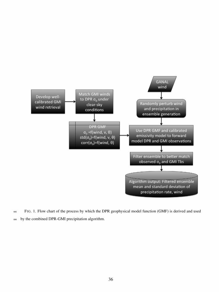
from rain-induced attenuation. Our strategy (Figure 1) is to develop a GMF for DPR based upon112

co-located GMI wind retrievals, and then use this GMF under raining conditions by modifying the113

combined GPM DPR-GMI precipitation retrieval algorithm CORRA (Olson and Masunaga 2015).114

In order to have as accurate a wind reference as possible, we evaluate three emissivity models after115

calculating offsets under clear and calm conditions to achieve consistency with the GMI calibra-116

tion. Next, we use all available matchups of GMI and DPR under non-precipitating conditions to117

develop the GMFs. This process is presented in section 2. Next, the use of GMFs in the GPM118

combined GMI-DPR ensemble filter retrieval framework, including validation of winds in regions119

of precipitation against buoy measurements, is described in section 3, followed by a summary in120

section 4.121

2. Development of Geophysical Model Functions for DPR122

Although physical models exist to describe the relationship between wind speed, the wave spec-123

trum, and backscatter (Durden and Vesecky (1985); Majurec et al. (2014)), the desire for GPM124

applications is to be as internally consistent as possible between the emissivity model and DPR125

GMF. Therefore, the strategy in this study is to derive empirical GMFs from clear-sky matchups126

of DPR and GMI-derived 10m wind retrievals, eliminating as much as possible the error from127

precipitation and cloud cross-talk described in section 1, then apply those GMFs to retrievals un-128

der all conditions. The use of empirical GMFs derived in this manner is standard practice in the129

scatterometer community (Migliaccio and Reppucci 2006).130

7

The first step in this process is to generate the clear-sky wind retrievals and then assess their error131

relative to buoy observations. In the absence of precipitation, the microwave radiances measured132

by GMI are primarily sensitive to the surface emission, atmospheric temperature and water vapor133

profile, and cloud liquid water. These parameters can be solved for using optimal estimation, also134

known as variational, retrieval techniques. These have been implemented for microwave sensors135

by Elsaesser and Kummerow (2008) and Boukabara et al. (2011), and a blend of their approaches is136

used to derive the surface and atmospheric properties from GMI by minimizing the cost function:137

J = (x−xa)T Sx

−1(x−xa)+(y− f (x))T Sy−1(y− f (x)). (1)

The components of the optimal estimation retrieval are the state vector (x) and covariance ma-138

trix (Sx), the observation vector (y) and covariance matrix (Sy), and forward model f (x). For139

water surfaces, the state vector consists of the 10m wind speed, cloud liquid water path, and a140

set of variables representing the values of the leading empirical orthogonal functions (EOFs) of141

the atmospheric temperature and water vapor profile. These EOFs were derived from 10 years142

of MERRA reanalysis (Rienecker et al. (2011); NASA/GMAO (2008)) independently in 1K SST143

bins. The number of leading EOFs is chosen such that at least 99% of the variance in temperature144

and water vapor is explained by the selected EOFs. The EOFS are used to simultaneously adjust145

the initial atmospheric temperature and water vapor profiles in order to match the observed GMI146

radiances. This is a change from the Elsaesser and Kummerow (2008) method, which assumed a147

constant lapse rate and scale height for water vapor. These assumptions are sufficient for matching148

observations near the 22-GHz water vapor absorption line, where radiances are mostly sensitive to149

the total column-integrated amount of water vapor and are less sensitive to its vertical structure and150

emitting temperature. However both the vertical structure of water vapor and temperature matter151

for modeling the additional channels near 183 GHz on GMI, so some method of adjusting the152

8

shape of the profile in mid and upper levels is necessary. The EOFs represent the climatological153

co-varying structures in temperature and water vapor profiles, and are a robust way to adjust both154

without requiring temperature sounding channels (e.g., 50-55 GHz). The a priori (and initial) state155

xa is the MERRA reanalysis interpolated in time and space to the GMI pixel location.156

Because the atmosphere is represented by EOFs and no covariance between the atmosphere and157

wind/cloud is assumed, the state covariance matrix Sx is diagonal. The observation vector consists158

of the 13-channel GMI radiances from the GMI Level 1C-R (intercalibrated and co-located) prod-159

uct (GPM Science Team 2015). The co-location matches the high-frequency (HF) observations160

(166V&H, 183±3, and 183±7 GHz), which are observed at 49.2◦ earth incidence angle, with the161

lower-frequency (LF) observations, which are observed at 52.8◦ earth incidence angle. A diagonal162

matrix for Sy is also assumed, with values of instrument noise (Hou et al. 2014) plus additional163

error determined from buoy matchups (Table 1) to account for forward model error and inexact164

footprint matching.165

The forward model is derived from the Community Radiative Transfer Model (CRTM) Emis-166

sion (non-scattering atmosphere) model, modified to include the downwelling path length cor-167

rection for roughened water surfaces as described by Meissner and Wentz (2012) and using the168

same atmospheric layers that are provided by MERRA products up to 10 hPA. Absorption by at-169

mospheric gases is calculated from Rosenkranz (1998) and Tretyakov et al. (2003). Cloud liquid170

absorption follows Liebe et al. (1991) and cloud water is assumed to follow an adiabatic profile171

(Albrecht et al. 1990). Since the surface emissivity and its relationship to wind speed is of funda-172

mental importance to this study, three emissivity models were tested for their ability to produce173

unbiased clear-sky radiances when forced with buoy-observed surface winds (within 30 minutes174

of a GPM overpass) and MERRA atmospheric profiles: FASTEM4/5 (as implemented in CRTM;175

9

Liu et al. (2011)) and the Meissner and Wentz (2012) (hereafter MW) model.1 Wind direction176

was not considered in this study as only the MW model is capable of representing wind direction-177

induced emissivity changes. Instead we include the wind-direction induced error in total model178

error which is derived from buoy matchups. The source of wind observations in this study is the179

International Comprehensive Ocean-Atmosphere Data Set version 2.5 (ICOADS; Woodruff et al.180

(2011); NCDC/NESDIS/NOAA (2011, updated monthly)) from April 2014-March 2015. Only181

observations from platforms with a known anemometer height (hb) were considered, and all winds182

were adjusted to 10m assuming neutral buoyancy using the relationship (Hsu et al. 1994):183

w10 = wb(10/hb)0.11. (2)

Before the emissivity models can be intercompared, sensor calibration must be considered. Fol-184

lowing Meissner and Wentz (2012), a calm-wind offset (δ0) was determined for each emissivity185

model and each GMI channel. These offsets were obtained by first selecting a subset of ICOADS186

observations with 10m winds less than 3.5 m s−1, where the emissivity-wind relationship is linear.187

To filter out clouds, observations were excluded if the polarization difference at 89 GHz was less188

than an SST-dependent threshold representing a cloud liquid water path of 0.01 kg m−2 under189

average atmospheric conditions or the spatial standard deviation (within 15 km) of 89 GHz Tb190

was greater than 2 K. The RTM was then forced with the observed SST and wind speed and in-191

terpolated MERRA atmospheric profile. The offsets were then calculated in order to minimize the192

bias between observed and simulated GMI brightness temperatures. No offsets were applied to193

the 183 GHz channels, as these were not sensitive to the surface emissivity in the matchups. The194

offsets and root-mean-square error (after offsets have been applied) are given for each channel195

and emissivity model in Table 1. The biases are different for each model at low frequencies, but196

similar or identical at 166 GHz, indicating low sensitivity of the brightness temperatures to emis-197

1Note that the MW model does not include frequencies higher than 90 GHz and FASTEM5 was substituted at these frequencies.

10

sivity at these channels and therefore low confidence in the offsets, which are likely influenced by198

the water vapor absorption model and/or absolute calibration of GMI. The root-mean-square-error199

(rmse) values, which are not sensitive to the choice of emissivity model, represent the error from200

other components of the forward model (such as wind direction and water vapor absorption) plus201

instrument noise, and are used as the diagonal components of Sy.202

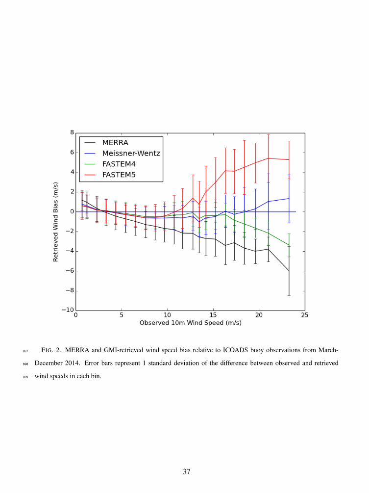
Next, each emissivity model was evaluated under the full range of conditions encountered in the203

GMI buoy overpasses. The retrieval was performed with each emissivity model and the retrieved204

winds are compared with observations in Figure 2. These results were filtered to remove precip-205

itation by applying a maximum threshold of 1.0 for the normalized cost function. It is apparent206

from these results that the MERRA analysis is biased high at observed wind speeds below 3 m s−1207

and biased low above this threshold. The retrievals using the different emissivity models behave208

similarly to each other up to about 8 m s−1 and remove most of this bias, but diverge due to differ-209

ent foam models (implicit in MW and explicit in FASTEM 4/5). At observed wind speeds greater210

than 15 m s−1, FASTEM4 begins to diverge below the observed wind speed whereas FASTEM5211

diverges above more severely. The MW model gives a slight low bias of as much as 1 m s−1 at212

10-15 m s−1 but recovers to near zero at higher speeds. The overall root-mean-squared error in213

clear conditions for the MW model is 1.3 m s−1 (equivalent to WindSat) and, because of its low214

bias over the range of observed wind speeds, is chosen to generate the DPR GMFs.215

The DPR GMF was generated by averaging the observed σ0 from the DPR Level 2 product216

(Iguchi and Meneghini 2014), removing the two-way attenuation from gases and cloud liquid217

water (which are determined from the GMI retrievals), in wind speed bins with 0.5 m s−1 spacing218

from 0 to 10 m s −1, 1 m s−1 spacing between 10 and 20 m s−1, and 2 m s−1 spacing above 20 m219

s−1. Note that all of the results presented in this manuscript are from observations taken between220

25 August 2014 (when the most recent phase shift code for DPR was implemented) and 30 April221

11

2015. Earlier observations used different phase shift codes and attenuator settings, which had some222

slight impact on the GMFs (not shown). The standard deviation in each bin is also calculated as is223

the correlation coefficient in the case of the matched KuPR-KaPR beams. The standard deviation224

serves as an implicit indicator of the quality of the derived GMF: Low values are desirable because225

they indicate that the 10m wind speed retrieved by GMI is sufficient to represent the sea state for226

the purposes of reproducing σ0, and, when used in the combined framework, provide a stronger227

constraint on the PIA contributed by the precipitation column. The theoretical minimum standard228

deviation of σ0 for DPR, assuming the signal-to-noise ratio is large (true under almost all non-rain229

conditions), depends on the number of independent samples, N, taken. If the surface is modeled230

as a Rayleigh target (an incoherent sum from many specular points on the surface without any231

dominant scattering contribution) and a logarithmic receiver is used, then the standard deviation232

in dB is given by (Sauvageot 1992):233

std(σ0) =5.57√

N, (3)

where N depends on incidence angle and varies between 100 and about 110 . Using these num-234

bers, the nominal standard deviation in σ0, from sampling alone, is a bit more than 0.5 dB.2235

Values higher than 0.5 dB could be caused by random errors in the GMI wind reference (this is236

compounded when the sensitivity of σ0 to wind is high) or that something other than wind speed237

is contributing the variation of σ0, resulting in diminished impact of the σ0 observation on the238

precipitation retrieval. In Figure 3, the standard deviation of σ0 for the KuPR, in normal scan (NS)239

mode, and KaPR, in matched-scan (MS) and high-sensitivity (HS) modes, is shown as a function240

of DPR incidence angle for three wind speed bins centered on 0.5 m s−1, 5 m s−1, and 15 m s−1.241

2For off-nadir incidence, where there are multiple samples from the surface, a case can be made for integrating over all the data from the surface.

This should reduce the standard deviation of the σ0; however, in the DPR processing, the σ0 is based on the peak return power, not the integrated

power.

12

At the low wind speed, the standard deviation is quite high (nearly 10 dB), particularly off nadir,242

but smaller (still 2-4 dB) near nadir at both frequencies (the lower Ku values are likely due to the243

saturation of the KuPR receiver). As the wind becomes calm, the surface is nearly specular and the244

sensitivity to small changes in wind speed is quite high off nadir, so random error in the reference245

wind is thought to primarily contribute to the large standard deviation there. Long-period swell246

also provides an increasing contribution to variation in σ0 (Tran et al. 2007) that is unrelated to247

the local wind speed. Finally, since the change in σ0 with respect to incidence angle is also high at248

low wind speeds, small changes in the incidence angle (the standard deviation of DPR incidence249

angle was around 0.01◦ in each angle bin) may also contribute to the high standard deviation at250

off-nadir angles.251

At moderate and high wind speeds, the standard deviations are much lower and the pattern252

is shifted slightly to relatively high values near nadir and at the largest off-nadir angles, with253

minima around 9◦ for KuPR. Specular effects can again explain the near-nadir maximum, whereas254

the off-nadir maxima are likely a result of wind direction sensitivity (Wentz et al. 1984). The255

KaPR standard deviations are slightly higher for the MS than the HS data due to the shorter pulse256

width, and are qualitatively similar to the KuPR data. The effect of more stringent quality control257

(reduction of the cloud LWP, its spatial variability, and cost function thresholds by 50%; denoted258

QC2 in Figure 3) is also most evident here in reducing the KaPR standard deviation, but the259

differences are negligible enough (0.01 dB) that the original thresholds (QC1) are used to generate260

databases for the combined algorithm as this choice of thresholds provides more data, especially261

at higher wind speeds.262

13

The two-dimensional GMFs of σ0 are shown in Figure 4. Most of the variability is exhibited263

at low wind speeds at both Ku and Ka bands3. However, σ0 continues to decrease near nadir for264

wind speeds as high as 30 m s−1, which is approximately the upper limit of the reliable data that265

has been collected so far. Off-nadir, σ0 appears to reach maxima at increasing wind speeds with266

incidence angle. The standard deviation of σ0 reaches minima near the 0.5 dB sampling limit267

at 5-15◦ and wind speeds between 5 and 10 m s−1. There is also a minimum in the standard268

deviation at Ku band (but not Ka band) at very low wind speeds near nadir. This is an artifact of269

the saturation of the Ku receiver when σ0 ≥ 22.5 dB (The Ka receiver saturates closer to 40 dB,270

which is only observed over some land and ice surfaces). The higher standard deviations at the271

off-nadir angles are likely a result of wind-direction induced variability in σ0. In Figure 4f the272

observed Ku-band σ0 is compared to the cutoff-invariant two-scale model (Soriano and Guerin273

2008) using the Durden-Vesecky single-amplitude wave spectra (Durden and Vesecky 1985). This274

model appears to produce a flatter σ0 when viewed with respect to incidence angle at low wind275

speeds, but at winds above about 8 m s−1 has a comparable shape to the observed GMF minus a276

small (1 dB) offset. These results are consistent with the comparisons of this model to airborne277

observations of σ0 reported by Majurec et al. (2014).278

The Ku-Ka σ0 correlation (Figure 4e) is an important component of the dual-frequency sur-279

face reference technique (DSRT; Meneghini et al. (2012)). In the DSRT, σ0 is replaced by the280

differential σ0:281

δσ0 = σ0(Ka)−σ0(Ku) (4)

and the method provides an estimate of the differential PIA, A(Ka)-A(Ku). The errors in both282

single-frequency SRT and DSRT methods are dominated by the fluctuations in the rain-free ref-283

3the Ka HS GMF is not shown, but is essentially identical to the MS data with a -0.2 dB offset owing to the inability of the larger pulse width

to capture the surface peak as effectively, especially near nadir.

14

erence data: σ0 and δσ0. As the correlation between σ0(Ku) and σ0(Ka) increases, the variance284

in δσ0 decreases so that the DSRT provides a potentially more accurate estimate of the path at-285

tenuations. The correlations, which are near 0.8 in most DPR angle bins when all wind speeds286

are considered, reduce to 0.1-0.4 for most wind speeds > 5 m s−1 and off-nadir incidence angles.287

This suggests that wind is responsible for most of the covariance in Ku and Ka σ0 but near-nadir288

and at low winds the stronger correlations make the DSRT technique particularly useful.289

3. Combined Radar-Radiometer Retrieval of Precipitation and Surface Wind290

The MW emissivity model (optimized for GMI) and DPR wind-σ0 GMFs described in section291

2 are implemented in the forward modeling component of the GPM Combined Radar Radiometer292

(CORRA) retrieval algorithm. A description of the radar component of this algorithm is given by293

Grecu et al. (2011) and a more complete description of the algorithm architecture can be found in294

the Algorithm Theoretical Basis Document (Olson and Masunaga 2015); for the purposes of this295

manuscript, a brief summary and example case are presented in this section followed by validation296

statistics. It is difficult to directly ascertain the improvement (if any) in rainfall estimates over297

ocean owing to the lack of reliable direct measurements, but the algorithm can be assessed as to298

how well the forward model matches GPM observations and buoy observations of wind speed.299

The impact on retrieved precipitation amounts is also shown in this section.300

a. Algorithm Description301

The CORRA algorithm uses an ensemble filter technique (Evensen 2006) to retrieve a set of pre-302

cipitation profiles that are consistent with observations from KuPR, GMI, and KaPR (where avail-303

able). The first step in this process is the creation of an ensemble of solutions that fit the observed304

KuPR reflectivity profile without any consideration of the GMI, KaPR, or KuPR σ0 observations.305

15

The randomly perturbed properties of each profile solution include the vertical profile of the hy-306

drometer particle size distribution (PSD) intercept parameter (Nw), degree of non-uniform beam307

filling ,the cloud liquid water profile, relative humidity, and 10m wind speed. For each solution,308

the associated Ku and Ka σ0, Ka reflectivities, and GMI radiances are calculated. The calculation309

of Ka reflectivity’s accounts for multiple scattering enhancements using the multiscatter library310

developed by Hogan and Battaglia (2008).311

The ensemble is then filtered using the observed Ku σ0, GMI radiances, and Ka reflectivities and312

σ0 (where available). This is done by constructing an nvar× nmemb vector Xens representing the313

ensemble variables to be updated, including the perturbed variables, e.g., Nw and 10m wind, and314

derived/forward modeled variables, e.g., precipitation rate and brightness temperature. A separate315

nobs× nmemb vector Yens consists of the forward modeled variables corresponding to the nobs× 1316

observation vector Yobs (R is the corresponding observation error), which contains the observed317

σ0, brightness temperatures, and Ka reflectivities. The ensemble state vector Xens is then updated318

using the sample covariance:319

Xens = Xens +CovXY(CovYY +R)−1(Yobs−Yens). (5)

The algorithm output is derived from the updated ensemble and includes both mean and standard320

deviations of the geophysical parameters of the ensemble and forward modeled observations. This321

update is done separately for the Ku-only full swath (denoted as NS in GPM products) and Ku+Ka322

inner swath (MS products).323

b. Example Case324

To illustrate the update process described by Eq. 5, the retrieval algorithm is applied to a GPM325

overpass of a developing cyclone off the eastern coast of the United State on 26 January 2015 (Fig-326

16

ure 5). This case provides an opportunity to examine the algorithm under a variety of precipitation327

and surface wind conditions.328

The correlations (calculated from the initial, unfiltered ensemble) between the each observation329

type and the surface rain rate, as well as the correlations between each observation type and the330

10m wind speed, are shown in Figure 6 for both radar frequencies and the horizontally-polarized331

GMI channels from 10-36 GHz (which are most sensitive to rain and wind over water surfaces).332

It is evident from these sensitivities that algorithm adjustments to precipitation rate in convective333

rain (echoes greater than 40 dBZ; purple colors in Figure 5) are mostly a response to the initial Ku334

and Ka σ0 error, whereas adjustments in stratiform rain are mostly a response to the Ka σ0 and335

GMI Tbs (note that in the heaviest rain, the correlation between rain rate and 36H Tb becomes336

negative as scattering dominates over emission). Note that in extremely heavy precipitation with337

large amounts of ice aloft, the variability of Ka σ0 due to multiple scattering begins to overwhelm338

the attenuation, and the correlation decreases. In these cases, the algorithm relies mostly on Ku σ0339

to adjust the initial ensemble rain rates. In light and moderate rainfall, the 10m wind adjustment340

is mostly a response to Ku σ0, especially away from the approximately 9◦ incidence angle at341

which Ku σ0 is insensitive to wind. Nevertheless there is some sensitivity of the 10 and 19 GHz342

radiances and Ka σ0 to wind under lighter precipitation. Due to the finite number of ensemble343

members, there are some spurious negative correlations between wind and the Tbs in heavier rain,344

but these are weak and do not substantially impact the output. The degree to which the ensemble345

spread is reduced after the filtering step is indicative of the overall information content in the346

observations for each variable of interest, and is provided as part of the standard CORRA output.347

17

c. Internal Validation348

Output from 400 GPM orbits between September 2014 and January 2015 are analyzed to assess349

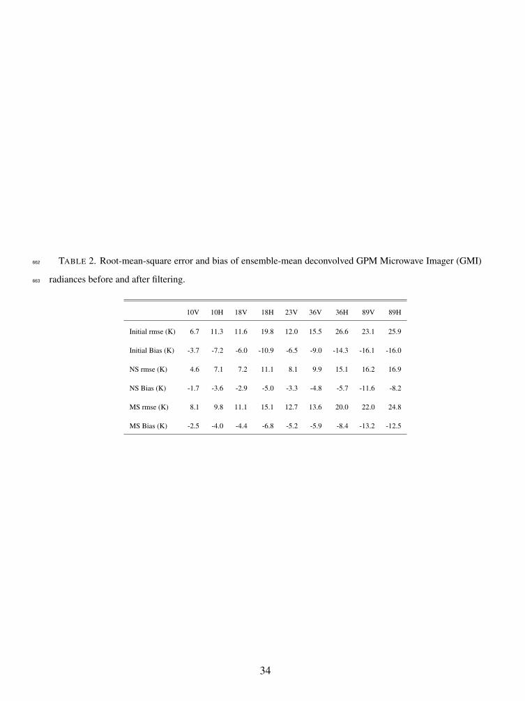
the internal consistency between the forward model and observations before and after filtering.350

The mean bias and root-mean-square (rms) error between the initial ensemble mean and filtered351

ensemble mean for both NS (Ku+GMI) and MS (Ku+Ka+GMI) are given in Table 2. There is a352

general cold bias to the initial simulated brightness temperatures (Tbs) at all frequencies (although353

a warm bias is present in the 18 and 36 GHz channels at rain rates exceeding 10 mm hr−1). Both354

the rms error and magnitude of the bias are reduced after filtering as expected. The MS error and355

bias are larger than the NS error and bias because the initial ensemble profiles are constrained by356

the additional Ka band information and are less free to be adjusted to match the GMI radiances.357

In other words, the NS retrievals are over-fit to the Tbs, which suggests an increase in their error358

values in R is warranted.359

The initial and filtered rms error and bias of σ0 is shown as a function of scan angle in Figure 7.360

There is a significant reduction in Ku rms error at all scan angles. The Ka error values are higher361

due to the stronger attenuation and multiple scattering effects, but errors are still reduced by nearly362

50% after the filtering step. The bias plots show a pattern of initial errors that are consistent with363

a low bias in the ENV wind (too high near nadir and too low off nadir). This bias appears to be364

more significant than any systematic bias in the precipitation attenuation, which would have the365

same sign regardless of scan angle.366

d. External Validation367

During September 2014-January 2015, 606 buoy observations from the ICOADS database were368

identified as being within 30 minutes of a GPM overpass and in the KuPR swath (308 of these369

18

were within the KaPR swath) at the same time that DPR detected precipitation in the pixel nearest370

to the buoy location. These observations were used to validate the CORRA wind retrieval.371

The wind rmse and bias are shown in Figure 8. Similar to the MERRA data analyzed in section372

2, these background winds are biased high below 3 m s−1 and biased low at higher wind speeds373

relative to the buoy observations. Root-mean-square errors increase from 2 m s−1 to 4 m s−1374

and NS errors are slightly higher than the MS or ENV errors. However, the bias is significantly375

reduced in the filtered datasets relative to the initial winds, indicating that while the retrievals are376

noisy, adjustments tend to be in the correct direction (this is consistent with the initial and filtered377

Tb and σ0 biases as well).378

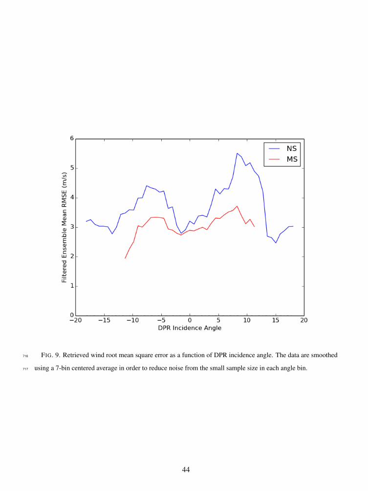
The wind error is shown as a function of incidence angle in Figure 9. It is evident that the379

largest errors occur near the 9◦ incidence angle where there is little sensitivity of σ0 to wind380

speed (Figures 4 and 6 illustrate this behavior). Near nadir and beyond 12◦ incidence angles, the381

sensitivity is stronger and the wind errors are much smaller. The NS errors are similar and the382

MS errors are smaller than the 4.26 m/s error of ASCAT under raining conditions (Portabella et al.383

2012) and 3.5 m/s error Quickscat retrievals using a neural network to compensate for rain effects384

(Stiles and Dunbar 2010). These are also within the range of 2 to 5 m/s accuracy (depending on385

rain rate) of a globally-applicable rainy-atmosphere WindSat wind retrieval algorithm (Meissner386

and Wentz 2009). When stratified by rainfall rate, wind speed errors are similar for light (< 1387

mm hr−1) and moderate (1 mm hr−1 < R < 10 mm hr −1) precipitation rates, but increase at388

heavier precipitation rates as the wind-induced variability in σ0 and brightness temperatures is389

overwhelmed by the precipitation effects.390

19

e. Impact on Precipitation Retrieval391

Although the retrieval of wind in precipitation is useful for many applications, one of the main392

purposes of this work is to improve the precipitation retrieval by enforcing an internal consis-393

tency between the surface emissivity (which depends on wind) and observed σ0 which depends394

on both wind and precipitation-induced path-integrated attenuation (PIA). In this section we show395

the impact of switching from the SRT PIA (which infers PIA by comparing the observed σ0 to a396

reference outside the precipitation) to the coupled σ0-emissivity model.397

Theoretically, the use of σ0 as an observation (instead of SRT-derived PIA) should impact the398

agreement between observed and modeled Tbs in two ways: First, through adjustments to the rain399

column to match the observed σ0 by changing the PIA, and second, via changes in the surface400

emissivity. The relative importance of these mechanisms depends on the relative sensitivity of401

the Tbs and σ0 to changes in the rain column and surface wind. Figure 10 shows the change402

in near-surface precipitation rate retrieved by the GPM combined algorithm over ocean surfaces403

equatorward of 55◦ latitude (to eliminate possible sea ice) when the SRT PIA (single frequency for404

NS retrievals in top panels; DSRT in the MS retrieval shown in the bottom panels) is replaced with405

the observed σ0 in the observation vector. Light precipitation (< 1 mm hr−1) is increased slightly406

in the NS swath, predominantly at wind speeds > 10 m s−1 and at incidence angles less than 12◦.407

The discontinuities in the 10-12◦ range are an artifact of the unavailability of the low-frequency408

GMI channels near the edge of the DPR swath (the deconvolution procedure requires coverage409

of the full footprint within the DPR swath). This suggests that GMI Tbs are driving the increase410

in precipitation, which is consistent with the weak Ku σ0-precipitation correlation in light rain411

(Figure 6). Near the edges of the DPR swath, where the GMI Tbs are not used, there is not enough412

20

information to significantly adjust the precipitation rate because the Ku-band PIA is small relative413

to the uncertainty in σ0, so the SRT and coupled method have the same information content.414

At moderate (1 mm hr−1 < R < 10 mm hr −1) precipitation rates, the wind-σ0 correlation is415

still larger than the rain correlation at Ku band whereas Tbs are more sensitive to the precipitation416

(although there is still some wind sensitivity especially at 10H). This results in some compensating417

behavior, where it is “easier” for the algorithm to increase the wind speed to satisfy the Ku σ0418

observation but must reduce the precipitation rate to be consistent with the Tbs. In heavy rain (>419

10 mm hr−1), the ensemble variance in σ0 and the Tbs is dominated by variance in the rain column,420

rather than surface wind, and where both observations are available only a very small reduction421

in precipitation is noted with the coupled forward model relative to the SRT method. When only422

Ku σ0 is available in the outer swath, however, there is a reduction in precipitation relative to the423

SRT version. The mean precipitation rate from the coupled model is more consistent across the424

different scan angles than the SRT version (not shown) which suggests that the SRT PIA may be425

biased high at the off-nadir angles and wind speeds from 5-10 m s−1.426

The Ku-Ka (MS) retrievals are generally more stable when comparing the SRT and coupled427

versions of the algorithm, but some changes are still notable. The increase in light precipitation428

is still present, but moderate and heavy precipitation show some different behavior from the NS429

retrievals with increases in light winds (below about 5 m s−1) and little change at higher wind430

speeds. There is not much sensitivity of Tb to wind at low wind speeds, so this appears to be431

driven by an increase in the inferred PIA in the coupled model relative to the dual-frequency SRT.432

4. Summary433

The Global Precipitation Measurement core satellite launched in February, 2014 carries a passive434

microwave imager (GMI) and dual-frequency radar (DPR) designed specifically to provide the435

21

most accurate instantaneous precipitation estimates currently available from space and serve as a436

reference for precipitation retrievals from other passive microwave imagers with similar channel437

sets (Kummerow et al. 2015). The GPM combined algorithm plays a key role in this process by438

providing precipitation estimates that are consistent with both GMI and DPR measurements. This439

algorithm uses physically-based forward models to simulate GMI and DPR measurements and it440

is desirable that those models use the same geophysical input parameters wherever possible.441

This study explored the feasibility of using internally consistent relationships between wind,442

emissivity, and backscatter for water surfaces in the combined algorithm. We first evaluated the443

FASTEM 4/5 (Liu et al. 2011) and Meissner and Wentz (2012) emissivity models in a GMI-only444

non-precipitation retrieval against buoy observations obtained from the ICOADS dataset. The445

Meissner-Wentz model provided the lowest root-mean-square error (1.3 m s−1) and was used446

to create a geophysical model function (GMF) for DPR Ku and Ka σ0 as a function of 10m447

wind speed and incidence angle by matching the GMI retrievals to DPR observations under clear448

conditions.449

The Meissner-Wentz emissivity model and DPR GMFs were then implemented in the GPM450

combined algorithm. This coupled forward model indicated that the sensitivity of σ0 to wind451

at Ku band dominates the precipitation sensitivity particularly in light to moderate rain and at452

low wind speeds, where the brightness temperatures are more sensitive to precipitation (although453

there is still some wind sensitivity, particularly at 10 and 18 GHz at horizontal polarization in454

light and shallow precipitation). Therefore, the surface reference (SRT) estimate of the DPR path-455

integrated attenuation (PIA) was replaced with σ0 in the observation vector. This is desirable456

because σ0 is directly observed by DPR while the SRT PIA includes implicit assumptions and457

can be unphysically negative in light rain. Because σ0 depends on both the 10m wind speed and458

22

attenuation from atmospheric gases, clouds, and precipitation, the 10m wind speed was added to459

the retrieval state vector.460

The combined wind/precipitation retrievals were then evaluated against the ICOADS buoy461

dataset under precipitating conditions, which have been a challenge for surface wind retrievals462

from standalone passive radiometers (e.g., WindSat) or scatterometers. Although the retrievals463

were noisier than under clear conditions (rmse of 3.7 m s−1 for Ku+GMI and 3.2 m s−1 for464

Ku+Ka+GMI), there was a significant reduction in the bias from the background data provided by465

GANAL (-10%) to the Ku+GMI (-3%) and Ku+Ka+GMI (-5%) retrievals. The impact on precip-466

itation retrievals was also evaluated. Ku+GMI retrievals of precipitation increased slightly on the467

light end (< 1 mm hr−1) and decreased in moderate to heavy precipitation (> 1mm hr−1) due to468

compensating effects of wind on σ0 and emissivity requiring changes in the precipitation column469

to maintain consistency with the observations. The Ku+Ka+GMI retrievals, being additionally470

constrained by the Ka reflectivity, did not change as much although a slight increase in moderate471

and heavy precipitation at low wind speeds was noted.472

While GPM was not designed specifically to measure ocean surface winds, this study demon-473

strates that such measurements are quite feasible in clear-sky conditions. In precipitation, using a474

coupled emissivity-backscatter GMF produces reasonable results that achieve the goal of internal475

consistency in the combined algorithm. The results presented here should only be considered as a476

proof of concept, as additional details that we did not consider, such as wind direction, the effect477

of rain on the scattering properties of water surfaces, and spatial correlation of the wind field, are478

left to future work.479

Acknowledgments. This work was supported under NASA Cooperative Agreement480

NNX12AD03A and Precipitation Measurement Missions Program Scientist Dr. Ramesh481

23

Kakar. We would also like to thank Dr. Thomas Meissner of Remote Sensing Systems for482

providing the computational codes for the Meissner-Wentz emissivity model, and Dr. Simone483

Tanelli of NASA JPL/CalTech for providing the cutoff-invariant two-scale Durden-Vesecky484

model data. Finally, we would like to thank the three anonymous reviewers whose comments and485

suggestions greatly improved the quality of this manuscript.486

References487

Albrecht, B. A., C. W. Fairall, D. W. Thomson, A. B. White, J. B. Snider, and W. H. Schu-488

bert, 1990: Surface-based remote sensing of the observed and the adiabatic liquid water489

content of stratocumulus clouds. Geophysical Research Letters, 17 (1), 89–92, doi:10.1029/490

GL017i001p00089, URL http://dx.doi.org/10.1029/GL017i001p00089.491

Battaglia, A., and C. Simmer, 2008: How does multiple scattering affect the spaceborne W-Band492

radar measurements at ranges close to and crossing the sea-surface range? Geoscience and493

Remote Sensing, IEEE Transactions on, 46 (6), 1644–1651, doi:10.1109/TGRS.2008.916085.494

Boukabara, S.-A., and Coauthors, 2011: MiRS: An All-Weather 1DVAR satellite data assimilation495

and retrieval system. Geoscience and Remote Sensing, IEEE Transactions on, 49 (9), 3249–496

3272, doi:10.1109/TGRS.2011.2158438.497

Donnelly, W. J., J. R. Carswell, R. E. McIntosh, P. S. Chang, J. Wilkerson, F. Marks, and P. G.498

Black, 1999: Revised ocean backscatter models at C and Ku band under high-wind con-499

ditions. Journal of Geophysical Research: Oceans, 104 (C5), 11 485–11 497, doi:10.1029/500

1998JC900030, URL http://dx.doi.org/10.1029/1998JC900030.501

Draper, D., D. Newell, F. Wentz, S. Krimchansky, and G. Skofronick-Jackson, 2015: The global502

precipitation measurement (GPM) microwave imager (GMI): Instrument overview and early on-503

24

orbit performance. IEEE Journal of Selected Topics in Applied Earth Observations and Remote504

Sensing, in review.505

Durden, S., and J. Vesecky, 1985: A physical radar cross-section model for a wind-driven sea506

with swell. Oceanic Engineering, IEEE Journal of, 10 (4), 445–451, doi:10.1109/JOE.1985.507

1145133.508

Elsaesser, G. S., and C. D. Kummerow, 2008: Toward a fully parametric retrieval of the nonraining509

parameters over the global oceans. J. Appl. Meteor. Climatol., 47, 1599–1618.510

Evensen, G., 2006: Data Assimilation: The Ensemble Kalman Filter. Springer, 280 pp.511

Fernandez, D. E., J. R. Carswell, S. Frasier, P. S. Chang, P. G. Black, and F. D. Marks, 2006:512

Dual-polarized C- and Ku-band ocean backscatter response to hurricane-force winds. Journal513

of Geophysical Research: Oceans, 111 (C8), n/a–n/a, doi:10.1029/2005JC003048, URL http:514

//dx.doi.org/10.1029/2005JC003048.515

Freilich, M. H., and B. A. Vanhoff, 2003: The relationship between winds, surface roughness, and516

radar backscatter at low incidence angles from TRMM Precipitation Radar measurements. J.517

Atmos. Oceanic Technol., 20, 549–562.518

GPM Science Team, 2015: GPM Level 1C R Common Calibrated Brightness Temperatures519

Collocated,version 04. NASA Goddard Earth Science Data and Information Services Cen-520

ter (GES DISC), Greenbelt, MD, USA, URL http://disc.sci.gsfc.nasa.gov/datacollection/GPM521

1CGPMGMI R V04.html, accessed 16 May 2015.522

Grecu, M., W. S. Olson, and E. N. Anagnostou, 2004: Retrieval of precipitation profiles from523

multiresolution, multifrequency active and passive microwave observations. J. Appl. Meteor.,524

43, 562–575.525

25

Grecu, M., L. Tian, W. S. Olson, and S. Tanelli, 2011: A robust dual-frequency radar profiling526

algorithm. J. Appl. Meteor. Climatol., 50, 1543–1557.527

Haddad, Z. S., E. A. Smith, C. D. Kummerow, T. Iguchi, M. R. Farrar, S. L. Durden, M. Alves, and528

W. S. Olson, 1997: The TRMM ‘Day-1’ radar/radiometer combined rain-profiling algorithm. J.529

Meteor. Soc. Japan, 75, 799–809.530

Hogan, R. J., and A. Battaglia, 2008: Fast lidar and radar multiple-scattering models: Part 2:531

Wide-angle scattering using the time-dependent two-stream approximation. J. Atmos. Sci., 65,532

3636–3651.533

Hou, A. Y., and Coauthors, 2014: The Global Precipitation Measurement Mission. Bull. Amer.534

Meteor. Soc., 95, 701–722.535

Hsu, S. A., E. A. Meindl, and D. B. Gilhousen, 1994: Determining the power-law wind-profile536

exponent under near-neutral stability conditions at sea. J. Appl. Meteor., 33, 757–765.537

Iguchi, T., T. Kozu, J. Kwiatkowski, , R. Meneghini, J. Awaka, and K. Okamoto, 2009: Uncertain-538

ties in the rain profiling algorithm for the TRMM Precipitation Radar. J. Meteor. Soc. Japan,539

87A, 1–30.540

Iguchi, T., T. Kozu, R. Meneghini, J. Awaka, and K. Okamoto, 2000: Rain-profiling algorithm for541

the TRMM Precipitation Radar. J. Appl. Meteor., 39, 2038–2052.542

Iguchi, T., and R. Meneghini, 2014: GPM DPR Level 2A DPR Environment V03 (GPM543

2ADPR), version 03. NASA Goddard Earth Science Data and Information Services Cen-544

ter (GES DISC), Greenbelt, MD, USA, URL http://disc.sci.gsfc.nasa.gov/datacollection/GPM545

2ADPR V03.html, accessed 8 April 2015.546

26

Kummerow, C. D., D. Randel, M. Kulie, N.-Y. Wang, R. Ferraro, S. J. Munchak, and V. Petkovic,547

2015: The evolution of the Goddard Profiling Algorithm to a fully parametric scheme. J. Atmos.548

Oceanic Technol., accepted.549

Li, L., E. Im, L. Connor, and P. Chang, 2004: Retrieving ocean surface wind speed from the550

TRMM Precipitation Radar measurements. Geoscience and Remote Sensing, IEEE Transac-551

tions on, 42 (6), 1271–1282, doi:10.1109/TGRS.2004.828924.552

Li, L., E. Im, S. L. Durden, and Z. S. Haddad, 2002: A surface wind model-based method to553

estimate rain-induced radar path attenuation over ocean. J. Atmos. Oceanic Technol., 19, 658–554

672.555

Liebe, H., G. Hufford, and T. Manabe, 1991: A model for the complex permittivity of water556

at frequencies below 1 THz. International Journal of Infrared and Millimeter Waves, 12 (7),557

659–675, doi:10.1007/BF01008897, URL http://dx.doi.org/10.1007/BF01008897.558

Liu, Q., F. Weng, and S. English, 2011: An improved fast microwave water emissivity model. Geo-559

science and Remote Sensing, IEEE Transactions on, 49 (4), 1238–1250, doi:10.1109/TGRS.560

2010.2064779.561

Majurec, N., J. Johnson, S. Tanelli, and S. Durden, 2014: Comparison of model predictions with562

measurements of Ku- and Ka-band near-nadir normalized radar cross sections of the sea sur-563

face from the Genesis and Rapid Intensification Processes experiment. Geoscience and Remote564

Sensing, IEEE Transactions on, 52 (9), 5320–5332, doi:10.1109/TGRS.2013.2288105.565

Meissner, T., and F. Wentz, 2009: Wind-vector retrievals under rain with passive satellite mi-566

crowave radiometers. Geoscience and Remote Sensing, IEEE Transactions on, 47 (9), 3065–567

3083.568

27

Meissner, T., and F. Wentz, 2012: The emissivity of the ocean surface between 6 and 90 GHz over569

a large range of wind speeds and earth incidence angles. Geoscience and Remote Sensing, IEEE570

Transactions on, 50 (8), 3004–3026, doi:10.1109/TGRS.2011.2179662.571

Meneghini, R., T. Iguchi, T. Kozu, L. Liao, K. Okamoto, J. A. Jones, and J. Kwiatkowski, 2000:572

Use of the surface reference technique for path attenuation estimates from the TRMM Precipi-573

tation Radar. J. Appl. Meteor., 39, 2053–2070.574

Meneghini, R., J. A. Jones, T. Iguchi, K. Okamoto, and J. Kwiatkowski, 2004: A hybrid surface575

reference technique and its application to the TRMM Precipitation Radar. J. Atmos. Oceanic576

Technol., 21, 1645–1658.577

Meneghini, R., L. Liao, S. Tanelli, and S. Durden, 2012: Assessment of the performance of a578

dual-frequency surface reference technique over ocean. Geoscience and Remote Sensing, IEEE579

Transactions on, 50 (8), 2968–2977, doi:10.1109/TGRS.2011.2180727.580

Migliaccio, M., and A. Reppucci, 2006: A review of sea wind vector retrievals by means of581

microwave remote sensing. Proceedings of the European Microwave Association Vol, 136, 140.582

Mitrescu, C., T. L’Ecuyer, J. Haynes, S. Miller, and J. Turk, 2010: Cloudsat precipitation profiling583

algorithm – model description. J. Appl. Meteor. Climatol., 49, 991–1003.584

Munchak, S. J., and C. D. Kummerow, 2011: A modular optimal estimation method for combined585

radar-radiometer precipitation profiling. J. Appl. Meteor. Climatol., 50, 433–448.586

NASA/GMAO, 2008: MERRA Reanalysis Data. NASA Goddard Earth Science Data and Infor-587

mation Services Center (GES DISC), Greenbelt, MD, USA, URL http://disc.sci.gsfc.nasa.gov/588

mdisc, accessed 27 February 2015.589

28

NCDC/NESDIS/NOAA, 2011, updated monthly: International Comprehensive Ocean-590

Atmosphere Data Set Release 2.5, Individual Observations. NOAA NCDC, Asheville, NC,591

USA, URL http://www1.ncdc.noaa.gov/pub/data/icoads2.5/, accessed 8 May 2015.592

Negri, A. J., R. F. Adler, and C. D. Kummerow, 1989: False-color display of Special Sensor593

Microwave/Imager (SSM/I) data. Bull. Amer. Meteor. Soc., 70, 146–151.594

O’Dell, C. W., F. J. Wentz, and R. Bennartz, 2008: Cloud liquid water path from satellite-based595

passive microwave observations: A new climatology over the global oceans. J. Climate, 21,596

1721–1739.597

Olson, W. S., and H. Masunaga, 2015: GPM Combined Radar - Radiometer Precipitation Al-598

gorithm Theoretical Basis Document (Version 3). NASA ATBD, NASA GSFC, 59 pp. URL599

http://pps.gsfc.nasa.gov/Documents/Combined algorithm ATBD.2014.restore16-1.pdf.600

Portabella, M., A. Stoffelen, W. Lin, A. Turiel, A. Verhoef, J. Verspeek, and J. Ballabrera-Poy,601

2012: Rain effects on ascat-retrieved winds: Toward an improved quality control. Geoscience602

and Remote Sensing, IEEE Trans. Geosci. Rem, 50 (7), 2495–2506.603

Quilfen, Y., C. Prigent, B. Chapron, A. A. Mouche, and N. Houti, 2007: The potential of604

QuikSCAT and WindSat observations for the estimation of sea surface wind vector under se-605

vere weather conditions. Journal of Geophysical Research: Oceans, 112 (C9), n/a–n/a, doi:606

10.1029/2007JC004163, URL http://dx.doi.org/10.1029/2007JC004163.607

Rapp, A. D., M. Lebsock, and C. Kummerow, 2009: On the consequences of resampling mi-608

crowave radiometer observations for use in retrieval algorithms. J. Appl. Meteor. Climatol., 48,609

1981–1993.610

29

Rienecker, M. M., and Coauthors, 2011: MERRA: NASA’s modern-era retrospective analysis for611

research and applications. J. Climate, 24, 3624–3648.612

Rosenkranz, P. W., 1998: Water vapor microwave continuum absorption: A comparison of613

measurements and models. Radio Science, 33 (4), 919–928, doi:10.1029/98RS01182, URL614

http://dx.doi.org/10.1029/98RS01182.615

Sauvageot, H., 1992: Radar meteorology. Artech House Publishers.616

Seto, S., and T. Iguchi, 2007: Rainfall-induced changes in actual surface backscattering cross617

sections and effects on rain-rate estimates by spaceborne precipitation radar. J. Atmos. Oceanic618

Technol., 24, 1693–1709.619

Soriano, G., and C.-A. Guerin, 2008: A cutoff invariant two-scale model in electromagnetic scat-620

tering from sea surfaces. Geoscience and Remote Sensing Letters, IEEE, 5 (2), 199–203.621

Stiles, B., and R. Dunbar, 2010: A neural network technique for improving the accuracy of scat-622

terometer winds in rainy conditions. Geoscience and Remote Sensing, IEEE Transactions on,623

48 (8), 3114–3122.624

Stiles, B., and S. Yueh, 2002: Impact of rain on spaceborne Ku-band wind scatterometer data. Geo-625

science and Remote Sensing, IEEE Transactions on, 40 (9), 1973–1983, doi:10.1109/TGRS.626

2002.803846.627

Tran, N., B. Chapron, and D. Vandemark, 2007: Effect of long waves on Ku-band ocean radar628

backscatter at low incidence angles using TRMM and altimeter data. Geoscience and Remote629

Sensing Letters, IEEE, 4 (4), 542–546, doi:10.1109/LGRS.2007.896329.630

Tretyakov, M., V. Parshin, M. Koshelev, V. Shanin, S. Myasnikova, and A. Krupnov, 2003:631

Studies of 183 GHz water line: Broadening and shifting by air, N2 and O2 and integral in-632

30

tensity measurements. Journal of Molecular Spectroscopy, 218 (2), 239 – 245, doi:http://dx.633

doi.org/10.1016/S0022-2852(02)00084-X, URL http://www.sciencedirect.com/science/article/634

pii/S002228520200084X.635

Uhlhorn, E. W., P. G. Black, J. L. Franklin, M. Goodberlet, J. Carswell, and A. S. Goldstein,636

2007: Hurricane surface wind measurements from an operational stepped frequency microwave637

radiometer. Mon. Wea. Rev., 135, 3070–3085.638

Weissman, D. E., B. W. Stiles, S. M. Hristova-Veleva, D. G. Long, D. K. Smith, K. A. Hilburn,639

and W. L. Jones, 2012: Challenges to satellite sensors of ocean winds: Addressing precipitation640

effects. J. Atmos. Oceanic Technol., 29, 356–374.641

Wentz, F. J., S. Peteherych, and L. A. Thomas, 1984: A model function for ocean radar cross642

sections at 14.6 GHz. Journal of Geophysical Research: Oceans, 89 (C3), 3689–3704, doi:643

10.1029/JC089iC03p03689, URL http://dx.doi.org/10.1029/JC089iC03p03689.644

Woodruff, S. D., and Coauthors, 2011: ICOADS Release 2.5: Extensions and enhancements to the645

surface marine meteorological archive. International Journal of Climatology, 31 (7), 951–967,646

doi:10.1002/joc.2103, URL http://dx.doi.org/10.1002/joc.2103.647

Yueh, S., W. Tang, A. Fore, G. Neumann, A. Hayashi, A. Freedman, J. Chaubell, and G. Lager-648

loef, 2013: L-band passive and active microwave geophysical model functions of ocean surface649

winds and applications to Aquarius retrieval. Geoscience and Remote Sensing, IEEE Transac-650

tions on, 51 (9), 4619–4632, doi:10.1109/TGRS.2013.2266915.651

31

LIST OF TABLES652

Table 1. Bias (before applying offsets) and root-mean-square error (after applying off-653

sets), in K, of clear-sky, nearly-calm wind (< 3.5 m s−1 ) simulated brightness654

temperatures forced with buoy observations of SST and 10m wind and MERRA655

atmospheric parameters. No offsets were applied to the 183 GHz channels. . . . 33656

Table 2. Root-mean-square error and bias of ensemble-mean deconvolved GPM Mi-657

crowave Imager (GMI) radiances before and after filtering. . . . . . . . 34658

32

TABLE 1. Bias (before applying offsets) and root-mean-square error (after applying offsets), in K, of clear-

sky, nearly-calm wind (< 3.5 m s−1 ) simulated brightness temperatures forced with buoy observations of SST

and 10m wind and MERRA atmospheric parameters. No offsets were applied to the 183 GHz channels.

659

660

661

FASTEM4 FASTEM5 Meissner-Wentz

Channel bias rmse bias rmse bias rmse

10.65V 1.6 0.8 0.6 0.7 -1.0 0.7

10.65H 2.9 0.9 -0.4 0.9 -0.7 0.9

18.7V 0.6 1.0 0.2 1.0 -0.5 1.0

18.7H 2.3 1.6 0.3 1.5 0.1 1.5

23.8V -0.5 1.5 -0.5 1.4 -0.6 1.4

36.64V 0.6 0.9 0.6 0.9 0.6 0.9

36.64H 2.9 1.6 2.1 1.6 1.3 1.5

89V -0.4 1.0 0.0 1.0 0.8 1.1

89H 1.5 2.2 2.5 2.2 1.7 2.2

166V -0.1 1.4 -0.3 1.4 -0.3 1.4

166H 0.1 2.8 0.2 3.1 0.3 3.2

183±3 -2.8 3.7 -2.8 3.6 -3.0 3.6

183±7 -0.7 1.8 -0.9 1.9 -1.0 1.9

33

TABLE 2. Root-mean-square error and bias of ensemble-mean deconvolved GPM Microwave Imager (GMI)

radiances before and after filtering.

662

663

10V 10H 18V 18H 23V 36V 36H 89V 89H

Initial rmse (K) 6.7 11.3 11.6 19.8 12.0 15.5 26.6 23.1 25.9

Initial Bias (K) -3.7 -7.2 -6.0 -10.9 -6.5 -9.0 -14.3 -16.1 -16.0

NS rmse (K) 4.6 7.1 7.2 11.1 8.1 9.9 15.1 16.2 16.9

NS Bias (K) -1.7 -3.6 -2.9 -5.0 -3.3 -4.8 -5.7 -11.6 -8.2

MS rmse (K) 8.1 9.8 11.1 15.1 12.7 13.6 20.0 22.0 24.8

MS Bias (K) -2.5 -4.0 -4.4 -6.8 -5.2 -5.9 -8.4 -13.2 -12.5

34

LIST OF FIGURES664

Fig. 1. Flow chart of the process by which the DPR geophysical model function (GMF) is derived665

and used by the combined DPR-GMI precipitation algorithm. . . . . . . . . . . 36666

Fig. 2. MERRA and GMI-retrieved wind speed bias relative to ICOADS buoy observations from667

March-December 2014. Error bars represent 1 standard deviation of the difference between668

observed and retrieved wind speeds in each bin. . . . . . . . . . . . . . 37669

Fig. 3. Standard deviation of σ0 in three wind speed bins: 0.5 m s−1 (top), 5 m s−1 (middle), and670

15 m s−1 (bottom). The different colors represent different frequencies, DPR modes (NS671

= Normal Scan, MS = Matched Scan, HS = High Sensitivity), and quality control of the672

reference wind. . . . . . . . . . . . . . . . . . . . . . . 38673

Fig. 4. The two-dimensional geophysical model functions (GMFs) of σ0, its standard deviation,674

Ku-Ka correlation, and difference between the Durden-Vesecky single-amplitude model and675

observations at Ku band are shown as a function of 10m wind speed and incidence angle. . . 39676

Fig. 5. False-color GMI composite and KuPR maximum column observed reflectivity at 2204 UTC677

26 January 2015. The GMI composite is from the 89 GHz V and H and 36 GHz V channels678

following the Negri et al. (1989) scheme. . . . . . . . . . . . . . . . 40679

Fig. 6. Correlations of Ku and Ka σ0 and 10.65, 18.7, and 36.6 GHz horizontally-polarized bright-680

ness temperatures to surface rain rate and 10m wind speed, derived from the initial ensemble681

of solutions to each radar profile. . . . . . . . . . . . . . . . . . 41682

Fig. 7. Root-mean-square error (a) and bias (b) of the initial and filtered ensemble mean σ0 as a683

function of incidence angle. . . . . . . . . . . . . . . . . . . . 42684

Fig. 8. Background (JMA Global Analysis GANAL; 2A-ENV) and retrieved wind root-mean-685

square error and bias relative to ICOADS buoy observations in precipitating pixels. . . . . 43686

Fig. 9. Retrieved wind root mean square error as a function of DPR incidence angle. The data are687

smoothed using a 7-bin centered average in order to reduce noise from the small sample size688

in each angle bin. . . . . . . . . . . . . . . . . . . . . . 44689

Fig. 10. Change in GPM combined algorithm precipitation, as a function of wind speed and in-690

cidence angle, when the Surface Reference Technique (SRT) path-integrated attenuation691

(PIA) is replaced with the observed σ0 in the observation vector and coupled σ0-emissivity692

model is used in the forward model. The ENV wind and SRT-based precipitation are used693

as reference values. . . . . . . . . . . . . . . . . . . . . . 45694

35

FIG. 1. Flow chart of the process by which the DPR geophysical model function (GMF) is derived and used

by the combined DPR-GMI precipitation algorithm.

695

696

36

FIG. 2. MERRA and GMI-retrieved wind speed bias relative to ICOADS buoy observations from March-

December 2014. Error bars represent 1 standard deviation of the difference between observed and retrieved

wind speeds in each bin.

697

698

699

37

FIG. 3. Standard deviation of σ0 in three wind speed bins: 0.5 m s−1 (top), 5 m s−1 (middle), and 15 m s−1

(bottom). The different colors represent different frequencies, DPR modes (NS = Normal Scan, MS = Matched

Scan, HS = High Sensitivity), and quality control of the reference wind.

700

701

702

38

FIG. 4. The two-dimensional geophysical model functions (GMFs) of σ0, its standard deviation, Ku-Ka

correlation, and difference between the Durden-Vesecky single-amplitude model and observations at Ku band

are shown as a function of 10m wind speed and incidence angle.

703

704

705

39

FIG. 5. False-color GMI composite and KuPR maximum column observed reflectivity at 2204 UTC 26

January 2015. The GMI composite is from the 89 GHz V and H and 36 GHz V channels following the Negri

et al. (1989) scheme.

706

707

708

40

FIG. 6. Correlations of Ku and Ka σ0 and 10.65, 18.7, and 36.6 GHz horizontally-polarized brightness

temperatures to surface rain rate and 10m wind speed, derived from the initial ensemble of solutions to each

radar profile.

709

710

711

41

FIG. 7. Root-mean-square error (a) and bias (b) of the initial and filtered ensemble mean σ0 as a function of

incidence angle.

712

713

42

FIG. 8. Background (JMA Global Analysis GANAL; 2A-ENV) and retrieved wind root-mean-square error

and bias relative to ICOADS buoy observations in precipitating pixels.

714

715

43

FIG. 9. Retrieved wind root mean square error as a function of DPR incidence angle. The data are smoothed

using a 7-bin centered average in order to reduce noise from the small sample size in each angle bin.

716

717

44

FIG. 10. Change in GPM combined algorithm precipitation, as a function of wind speed and incidence angle,

when the Surface Reference Technique (SRT) path-integrated attenuation (PIA) is replaced with the observed

σ0 in the observation vector and coupled σ0-emissivity model is used in the forward model. The ENV wind and

SRT-based precipitation are used as reference values.

718

719

720

721

45