Page 1
A CONTINUATION ALGORITHM FOR PIECEWISE-LINEAR ANALYSIS
OF NONLINEAR RESISTIVE NETWORKS
by
SHUEH-MIEN LEE, B.S.E.
A THESIS
IN
ELECTRICAL ENGINEERING
Submitted to the Graduate Faculty of Texas Tech University in Partial Fulfillment of the Requirement for
the Degree of
MASTER OF SCIENCE
IN
ELECTRICAL ENGINEERING
Approved
Chairman"of the Committee
"^
^^JWI/IAJ^
May, 1980
Page 2
ACKNOWLEDGEMENTS
I am deeply indebted to Professor Kwong Shu Chao for his
direction of this thesis and to the other members of my committee.
Dr. Donald Gustafson and Dr. A. K. Mitra, for their helpful
criticism. I am also happy to thank my wife and my family for
the constant encouragement throughout this study.
UL
Page 3
TABLE OF CONTENTS
ACKNOWLEDGEMENTS ii
LIST OF FIGURES v
I. INTRODUCTION 1
II. MULTIPLE SOLUTIONS AND SOLUTION CURVE DEFINED
BY A RELATED DIFFERENTIAL EQUATION
2.1 Introduction 4
2.2 Iterative Solution Method 4
2.3 Existence and Uniqueness of Solution Curve . 7
III. MULTIPLE SOLUTIONS AND SOLUTION CURVE DEFINED
BY A CONTINUOUS PIECEWISE-LINEAR FUNCTION
3.1 Introduction 9
3.2 Piecewise-linear Approximation 10
3.3 Dynamic Behavior of Solution Curves . . . . 13
3.4 Starting Point 21
3.5 Numerical Algorithm 23
IV. CORNER PROBLEM AND THE PROBLEM OF SINGULAR
JACOBIAN MATRICES
4.1 The Comer Problem 30
4.2 Singular Jacobian Matrices Problem 32
V. APPLICATIONS
5.1 Piecewise-linear Analysis of AC Resistive
Network 36
1X1
Page 4
5.2 Driving-Point or Transfer-Characteristic Plots
of Multivalued Resistive Nonlinear Networks . . . 41
VI. CONCLUSION 45
LIST OF REFERENCES 47
iv
Page 5
LIST OF FIGURES
Figure Page
3.1. Nonlinear resistive network 11
3.2. The Ebers-Moll Model of a PNP transistor 11
3.3. A solution curve determined by Katznelson's algorithm 13
3.4. A solution curve crosses the boundaries 19
3.5a The circuit of example 3.1 24
3.5b The piecewise-linear approximation of function h for
the tunnel diode 25
3.6. The regions in the x-space 26
3.7. Solution curves of example 3.2 27
3.8. The circuit of example 3.2 28
3.9a The characteristic of a nonlinear element 28
3.9b The characteristic of a nonlinear element 28
3.10. The solution curve of example 3.2 29
4.1. The solution curve hits a corner 31
4.2. The solution curve enters a singular region 33
5.1. The circuit of example 5.1 38
5.2. Output voltages for different starting podjits 39
5.3. Output currents for different starting points 40
5.4. Multivalued input-output plot for the circuit in
example 5.2 43
5.5. Multivalued input-output plot for the circuit in
example 5.2 44
V
Page 6
CHAPTER I
INTRODUCTION
One of the most basic problems in the area of nonlinear circuit
analysis is the determination of the solutions (equilibrium points)
of nonlinear resistive networks. Research in nonlinear resistive
networks serves as a prerequisite to the understanding of general
nonlinear circuits and systems. This problem is important not only
from a circuit theoretic point of view but even more so from a com
putational point of view. Indeed, an essential part of most nonlinear
transient analysis computer programs is a DC analysis subprogram
[l-3]. In addition, similar problems are encountered in many related
fields such as mathematical economics, flow networks, power systems,
and least-square approximations.
Much work has been done in obtaining multiple solutions of
resistive nonlinear networks [4-9]. Some effort has been devoted
to using the technique of piecewise-linear approximation of a non
linear function [10-16]. For example, in the analysis of a elec
tronic circuit, diode and transistor characteristics can be repre
sented by continuous linear segments. This often gives considerable
insight to the problem and yields quick solutions. In general, by
peicewise-linear approximations, a nonlinear resistive network can
be characterized by the equation
f(x) = y (1.1)
where f(.) is a continuous piecewise-linear mapping of the real
Page 7
2
n-dimentional Euclidean space R into itself, x is a point in R and
represents a set of chosen variables of a given network and y is an
arbitrary point in R and represents the inputs. Usually, f(.) is
expressed in the form
f(x) = J ' x + w^^^ = y i = 1, 2, , N (1.2)
where J is a constant nxn matrix called the Jacobian matrix and
w is a constant n-vector, both defined in region R . The whole
space R is divided into a finite number N of polyhedral regions
by a finite number of hyperplanes.
Although various techniques have been deveolped for solving
piecewise-linear equations, relatively little has been done in
locating multiple solutions. It is the purpose of this thesis to
develop a systematic search technique for obtaining multiple soluti
ons of (1.1). The continuation method devised by Chao, Liu, and
Pan [4J plays an important role in the scheme developed in this
report.
For convenience and to make the present thesis self-contained,
the continuation method [4] is outlined in Chapter II. In Chapter
III, the general theory of the new algorithm is developed with two
assumptions, namely, all Jacobian matrices may have arbitrary signs
but are not singular and the solution curves never hit a comer.
The dynamic behavior of the search curve is discussed. Approaches
showing how a solution curve can be reached are presented. Formu-
Page 8
lation of equation (1.1) is also briefly introduced.
In Chapter IV, the corner problem and the problem of singular
Jacobian matrices are considered. Applications to other fields are
discussed in Chapter V. These include AC nonlinear resistive network
analysis and driving point or transfer characteristic curves of mul
tivalued nonlinear resistive networks. Finally, some concluding
remarks are given in Chapter VI.
Page 9
CHAPTER II
MULTIPLE SOLUTIONS AND SOLUTION CURVE DEFINED
BY A RELATED DIFFERENTIAL EQUATION
2.1 Introduction
The system of nonlinear equations is written as
g(x) = y (2.1)
or f(x) = g(x) - y = 0 (2.2)
where f or g is a continuous differentia le function from R onto
itself, X and y are both n-dimensional vectors to represent a set
of chosen variables and the inputs respectively.
A systematic search method has been developed by Chao, Liu
and Pan for locating multiple solutions of (2.2). For convenience,
this method is outlined here.
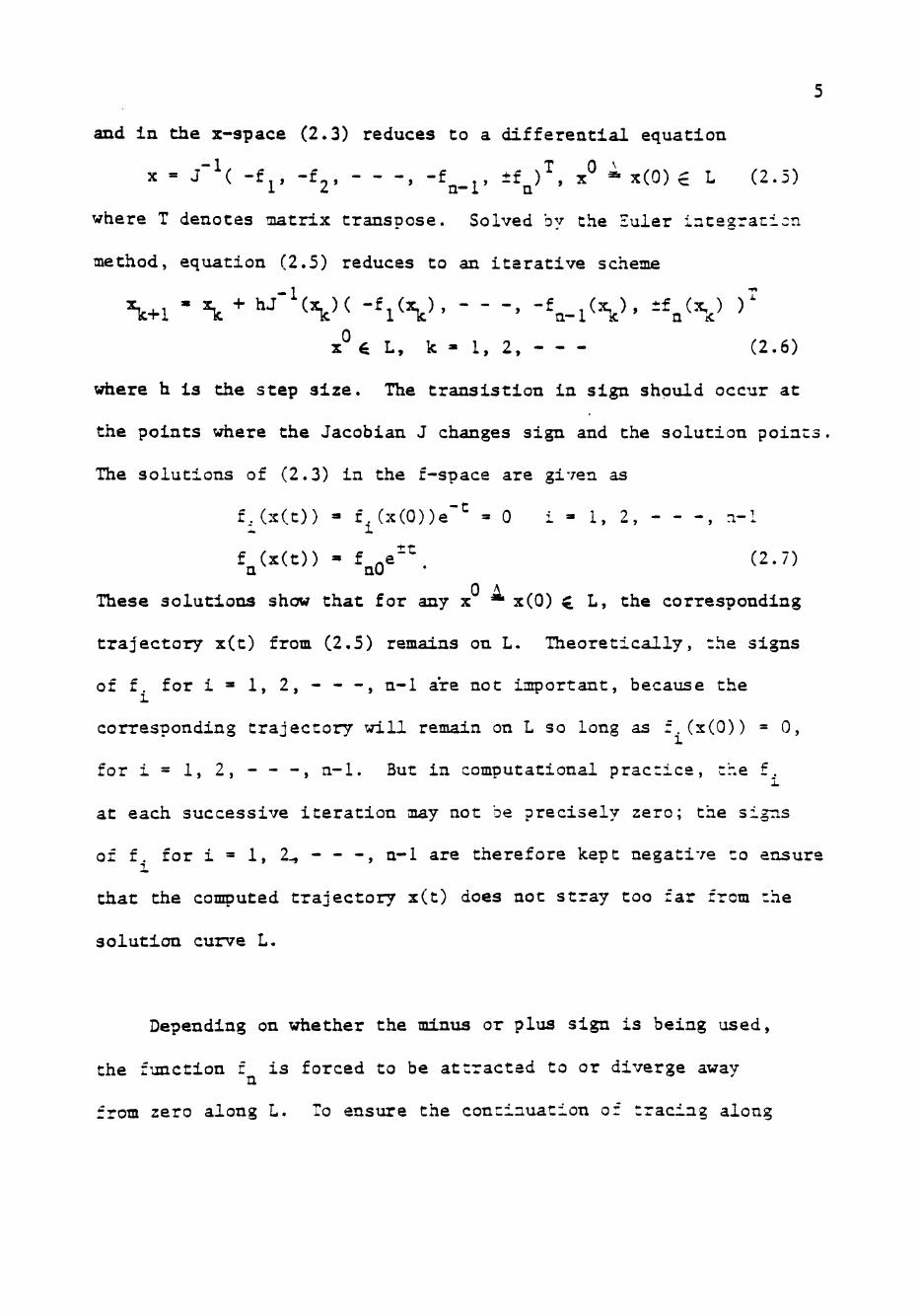
2.2 Iterative Solution Method
Consider a system of differential equations of the form
^ f.(x(t)) = -f,(x(t)) , f,(x(0)) = 0 i = 1, 2, , n-1 dt 1 1 1
where the initial conditions in f. are such that the starting point
X must lie on a space curve L of intersection f.(x) = 0 , i = 1, 2,
- - -, n-1. Since f is not a function of t explicitly, -r— can be dt
written as
dt ax dt "
Page 10
and i n the x-space (2.3) reduces to a d i f f e r e n t i a l equat ion
X = J""^( -f , , - f , . , - f , , ±f ) ^ , iP ^ x(Q)e L (2.5) i ^ n—i n
where T denotes matrix transpose. Solved by the Zuler intsgraticn
method, equation (2.5) reduces to an iterative scheme
\ ^ l ' \ ^ hJ- x )( -f (x ), - - -, -f .,(V> ^n^V )'
x^ L, k - 1, 2, (2.6)
where h is the step size. The transistion in sign should occur at
the points where the Jacobian J changes sign and the solution points.
The solutions of (2.3) in the f-space are given as
f,(x(t)) = f^(x(0))e'^ = 0 i - 1, 2, , n-1
0 A. These solutions show that for any x * x(0) L, the corresponding
trajectory x(t) from (2,5) remains on L. Theoretically, the signs
of f, for i » l , 2,---,n-l are not important, because the
corresponding trajectory will remain on L so long as f.(x(0)) = 0,
for i = l , 2 , - - - , n-1. But in computational practice, t"r.e f. 1
at each successive iteration may not 'oe precisely zero; the signs
of f. for i = 1, 2-, - - -, n-1 are therefore kept negative to ensure
that the computed trajectory x(t) does not stray too far from the
solution curve L.
Depending on whether the minus or plus sign is being used,
the function f is forced to be attracted to or diverge away n
from zero along L. To ensure the continuation of tracing along
Page 11
the solution curve L, the sign of f has to be changed at the
solution points of (2.2) and the points on L where the Jacobian
changes sign. The key point lies in a relation between the
determinant of Jacobian J and the directional derivative of f n
in the tangential direction of L
f = ^n = s^(Vf ) (2.8) ^ 3L~
where s is the unit vector in the tangential direction of L
and Vf is the gradient of f (x). The following theorems [4]
determine the conditions of the sign change of f .
Theorem 2.1; If f'(x) is the directional derivative of f (x) n n
in the tangential direction of L at x defined by
f,(x) = 0 , i = 1, 2, n-1 (2.9)
and A., is the (ij)th cofactor of the Jacobian matrix J of
f = (f^, f^, , f^)^, then
f' = det J / I I V I I n
where ||.|| denotes the Euclidean norm and
T ' = ( nl- ^ 2 - 'nr?
Theorem 2.2: The directional derivative of f^(x) in the tangential
direction of L changes sign if and only if the corresponding
Jacobian of f on L changes sign.
Other aspects concerning the convergence of the method and
starting point problem are also detailed in [4j.
Page 12
2.3 Existence and Uniqueness of Solution Curve
Success in finding all multiple solutions depends hea-vily on
whether (2.9) defines a unique simple curve L. If L is a simple
curve, i.e., a continuously differentiable curve which does not
intersect itself, then a complete tranversal of it enables one to
find all the multiple solutions. On the other hand, if L contains
several branches, then application of the method may lead to those
solutions that lie on the branch containing this starting point only.
The following theorems gives some sufficient conditions for the
existence and uniqueness of the solution curve [9].
Theorem 2.3: Let f be a real function of n real variables and of
class C . If
(i) det J never vanishes
and (ii) Lim | | f (x) | | = «, as x -»- °°
then any (n-1) equations off. = 0 , i = l , 2 , - - - , n defines a
unique continuously differentiable space curve.
T Theorem 2.4: Let h(x) = ( fj^(x), f2(x), , f^-l^^^ ^ ^® °^
class C . If there exists an (n-1) vector
x_ = ( ^v ^2' - -' \-l' \+l' - -' \ ^^ ^" """ k, 1 <. k < n,
such that
(i) T— is nonsingular for all x, and dX .
-k (ii) Lim | |h(x) [ | = «, as x , ->• °°
then h(x) = 0 defines a unique simple curve L.
Page 13
8
Definition: Let U C R • An n x n matrix A(x) is said to be almost
positive definite on U if A(x) is positive definite for all x
in U except at most a set of isolated points on which A(x) is
positive semidefinite.
Theorem 2.5: Let f:R ^R be a C function. If J(x) is almost
positive definite on R , then any (n-1) equations of f. = 0,
i = 1, 2, , n define a unique continuous space curve.
Theorem 2.6: Let f:R->R,n?^2, b e a C map. Let
S = {x^R^I det J(x) = 0} and T = {x € R^ j x e S}
If (i) det J(x) > 0 (or det J(x) < 0 ) for all x^T
and S is at most a set of isolated points,
(ii) limi I f (x) II = °° , as | | x | | - «
then any n-1 equations o f f . = 0 , i = l , 2, - - - , n define
a unique continuous space curve.
Page 14
CHAPTER III
MULTIPLE SOLUTIONS AND SOLUTION CURVE DEFINED
BY A CONTINUOUS PIECEWISE-LINEAR FUNCTION
3.1 Introduction
In chapter II a systematic search method for solving multiple
solutions of (2.2) is outlined. Considerable computation time is
needed to completely traverse the solution curve, and the success in
finding all the multiple solutions depends heavily on whether or not
the set of equations f.(x)=0, i = l , 2 , - - - , n-1 defines a simple
curve L, i.e., a continuously differentiable curve which does not
intersect itself.
Instead of sol-vrLng a system of nonlinear equations, the piecewise-
linear approximation is obtained for all the nonlinear elements in
a network. As a result, a set of piecewise-linear equations (1.1)
is to be solved. A method due to Katznelson ElO] was originally
applied only to the networks with 2-terminal elements which are
strictly monotonic. Fujjsawa and Kuh [ll] showed that if f is homeo-
morphic then the algorithm due to Katznelson always converges. Here
a continuous function f is said to be homeomorphic from R onto
itself if and only if the equation f(x) = y has a unique solution for
all y.
Kuh, Ohtsuki, Fujjsawa Il23 have shown that as long as all
the Jacobian matrix determinants det J , i = l , 2, - - - - , N
Page 15
10
in (1.2) have the same sign, there exists at least one solution to
the equation f(x) = y and the Katznelson's algorithm also converges.
This property is refered as the sign condition. Kuh and Chien [l3]
removed the restriction of the sign condition and demonstrated that
if all the Jacobian determinants in the unbounded region have the
same sign, the equation (1.1) has at least one solution. Chien has
also developed an algorithm that the domain of the x-space is divided
into simplices and the beha-vior of the system is approximated by a
linearized system in each simplex [l3]. Chua [l5] also introduced an
iterative scheme for finding multiple solutions. However, the method
is not suitable for networks with a large number of nonlinear elements.
In the following sections, a formulation of (1.2) and a systematic
search method for obtaining its multiple solutions are presented,
where the Jacobian matrices can have abitrary sign. A theoretical
basis for the development of the method is also given.
3.2 Piecewise-linear Approximation
The Taylor series expansion provides the analytic basis for
obtaining the piecewise-linear approximation. If the characteristic
of a nonlinear multiport is given by
z = h(x) (3.1)
then h(x) = h(xQ) -H | | | ^ ^ ^ ( X - X Q ) = J ( X Q ) X + w^ 3 ^
where J(x^) = T~| ^ cl w is a constant vector. (J dX I XFX_ U
Page 16
II
In the case of 2-terminal elements without coupling, this
reduces to the familiar tangent approximation. The Jacobian at
X- denoted by JCX-.) becomes the slope of the nonlinear function
at X-. and w. becomes the vertical axis intercept of the approximate
line segment. If the network contains n nonlinear resistive
elements, each characterized by an n -segment v.
there are N distinct segment combinations where n
i. curve, then 3
N ^ ^ ^
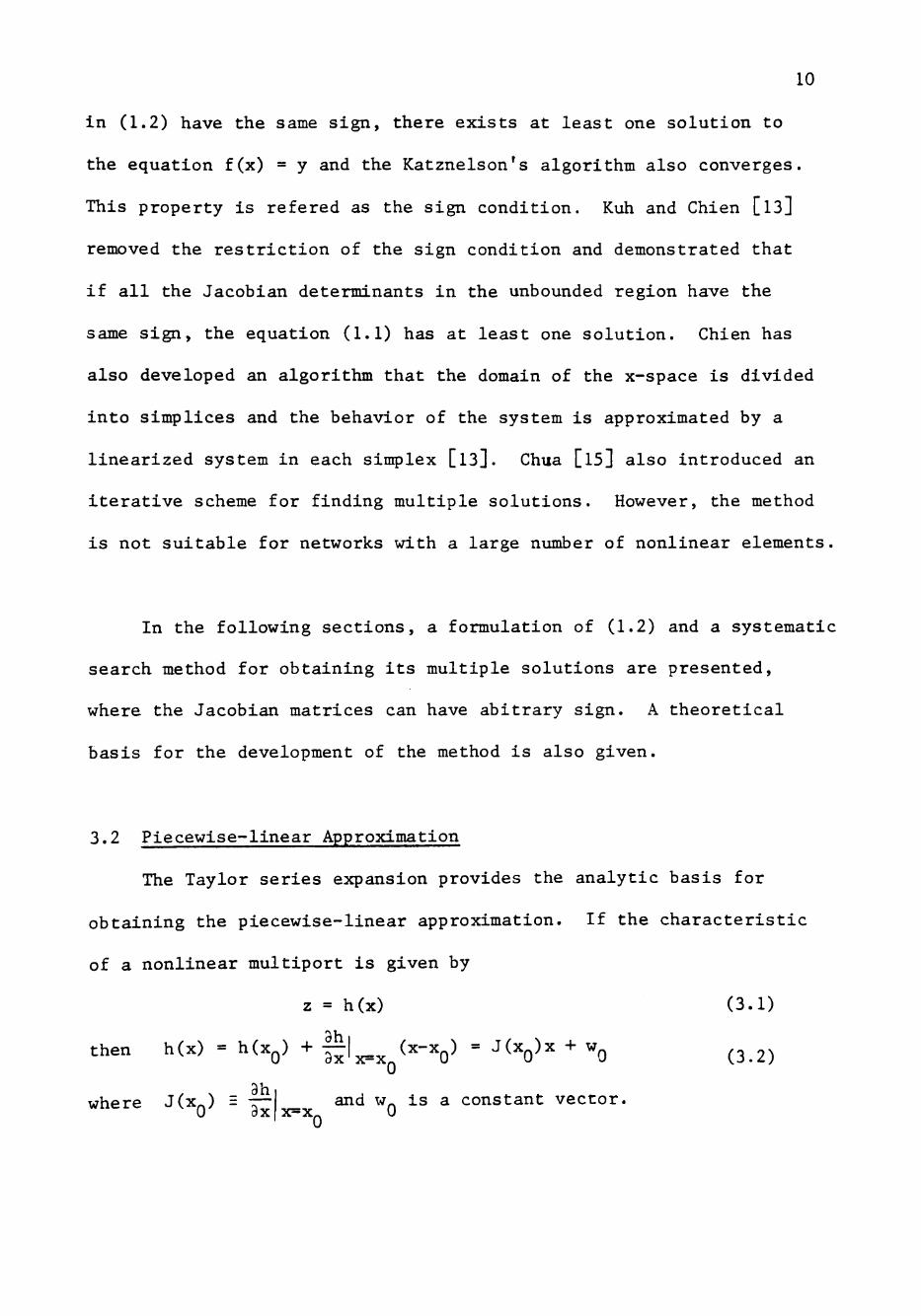
Consider a typical resitive nonlinear network as shown symbloicailv
in Fig 3.1 where the n nonlinear elements have been extracted and
are connected across the ports of a linear n-port network. As
indicated by So [17] and Chua [l5]. Fig 3.1 can be completely
characterized by an n x n hybrid matrix A and an n x 1 source vector
u, namely
Ax + u C3.4}
where the components of the n x 1 port vectors 2 and x can be any
combination of port voltage and port current pro-vided that the
corresponding components of 2 and x have the same port number.
N
Linear
Resistive
Network
^
i '1
1-7
m \
^U"^T^22
- ^
• 1 1
hi'^f^u
-• c
ao
^nn <
"vT,
Fig. 3.1 Nonlinear resistive network
rig. 3.2 The Toers—Moll model of a ?">!? transistor
Page 17
12
If each nonlinear resitive element is either voltage controlled of
current controlled, then (3.4) can be written in the form
z(x) = Ax + u (3.5)
before applying piecewise-linear approximations where
T n
z(x) = (z.(x), z„(x), , z (x)) is a nonlinear mapping from R
into R and z.(x) represents the nonlinear characteristics of the
ith nonlinear resistor. In either case, the terminal constraint
imposed by n nonlinear resistors can be expressed by its piecewise-
linear approximation, which is substituted for z in (3.4) or (3.5).
But the piecewise-linear approximation of multiterminal
elements with coupling is much more complicated. Fortunately, most
of coupling elements are of the type that can be expressed as sums
of nonlinear functions V7ith simple variables such as n
z.= E h..(x.) j = 1,2, , n -J 1 = 1 -•
= J^h'..(x.„) + «0 (3.6)
wh ere h'. .(x.^) is the slope of the function h.,(.) at x. ji lO Ji lU.
by ^e = ES< ^ T - » -"r^Cs( ^ - '^
For example, the Ebers-Moll model of a PNP transistor is represented
eb/v^ , r r ^ cb/v^ _ ^
(3.7)
^ = -,I,3( > / ^ ^ - ^ ) - ^CS^^'^''^^ - ^ >
The equivalent circuit model is shown in Fig (3.2) where
^22 = ^CS( ^^"^'"^ - ' ^ ' ^22(\b> ^'-'^
e " hi " V 2 2 "" c ' f ll * 22 ' •^
Page 18
13
Fig. 3.3. A solution curve determined by Katznelson's algorithm
Therefore, by specifying the piecewise-linear approximation
to all the nonlinear elements in the circuit, it is clear that
within each region the equation is linear and is of the form
f(x) = J^^^x + w^^^ = y i = 1, 2, ,N (3.10)
where J is a constant nxn matrix, y is the input vector.
The domain of f(.) in R is divided into N polyhedral regions
by a finite number of hyperplanes (or boundaries). A typical
boundary in the x-space can be characterized by the equation
n^x = 0 (3.11)
where n is the normal vector of the hyperplane (or boundary)
and c is a real constant. In (3.10), for example, if x is the
node-to-datum voltage vector and y is the input current source
vector, then J is the node admittance matrix.
3,3 Dynamic Behavior of Solution Curves
Let R , R be continuous regions with a common boundary charac-
Page 19
14
T
terized by the hyperplane n x = c. Since f is continuous piecewise-
linear, there exists an n-vector r such that
j(l) . j(j) = ,J (3 3)
where J and J ^ are Jacobian matrices of adjacent regions R
and R respectively.
Consider the continuous piecewise-linear equation
f(x) = J ^ x + w^ = y, i = 1,2, , N
where y is a given input. Fig. 3.3, a continuous curve in the
x-space is determined, based on Katznelson's algorithm
x^(X) = x^ + AJ ^ (y - y= )
where
i (i) i i y = J X + w
and X is a scalar parameter, If X = 1, then
i/iN 1 ^ r(l) f T(i) 1 1\
x ( l ) = x + J (y-J x - w )
= J ^ (y-w^).
It is clear that x (1) is a desired solution if it happens to be
in R" . Otherwise, the value of X has to be determined such that
x"''(X) lies on the boundary of R and R . Such a value of X is
denoted by X^. Define x^ = x^(X^) and y" = f(x ), the line
segment connecting x and x is then a portion of the desired
solution curve. We may extend the solution curve beyond x into
R""" in the similar manner.
Page 20
15
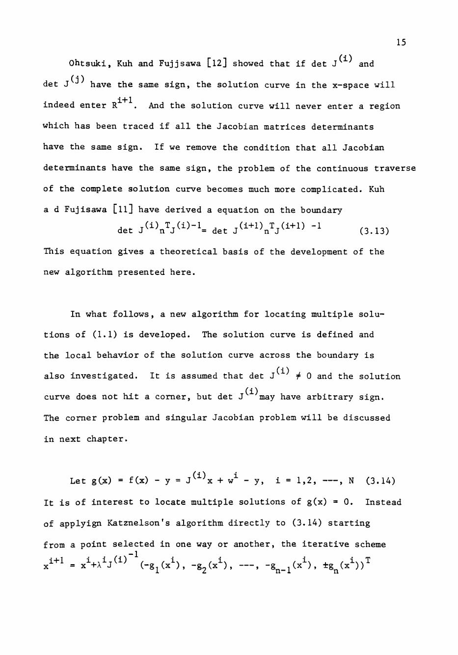
ohtsuki, Kuh and Fujjsawa [l2] showed that if det J and
det J -" have the same sign, the solution curve in the x-space will
indeed enter R . And the solution curve will never enter a region
which has been traced if all the Jacobian matrices determinants
have the same sign. If we remove the condition that all Jacobian
determinants have the same sign, the problem of the continuous traverse
of the complete solution curve becomes much more complicated. Kuh
a d Fujisawa [ll] have derived a equation on the boundary
det j(i>n^j("-l= det A^^'K'"/'^'^ "^ (3.13)
This equation gives a theoretical basis of the development of the
new algorithm presented here.
In what follows, a new algorithm for locating multiple solu
tions of (1.1) is developed. The solution curve is defined and
the local behavior of the solution curve across the boundary is
also investigated. It is assumed that det J ^ 0 and the solution
curve does not hit a comer, but det J may have arbitrary sign.
The comer problem and singular Jacobian problem will be discussed
in next chapter.
Let gCx) = fCx) - y = J ^ x + w^ - y, i = 1,2, , N (3.14)
It is of interest to locate multiple solutions of g(x) = 0. Instead
of applyign Katznelson's algorithm directly to (3.14) starting
from a point selected in one way or another, the iterative scheme
i+1 i,,i..(i) . . i. , iv / i\ . / INNT X = X +X J (-g (x ), -g2(x ), , -gj . Cx ), *g^(x ))
Page 21
16 x^ € L, i - 0 , 1 , 2 , (3.15)
i s used where the s t a r t i n g po in t x must l i e on a space curve L of
i n t e r s e c t i o n g . (x) = 0 , i = 1,2, , n-1 and X^ > 0 i s the l a r g e s t
p o s i t i v e number such t h a t x and x are in the same reg ion .
0 1 2 As long as X i s chosen to l i e on L, the i t e r a t i o n po in t s x , x ,
~ — remain on L.
Lemma 2.1: If x lies on a space curve L defined by g (x) * 0
1 2 i = 1,2, , n-1, then the successive points x , x , resulted
from (3.15) and the.'line segments joining these points also lie
on L.
Proof: Without lo s ing g e n e r a l i t y , assume x € L i s in region R .
Consider the following d i f f e r e n t i a l equat ion in R
4 r g . ( x ( t ) ) = - g , ( x ( t ) ) , g , (x (0 ) ) = 0, i = 1,2, , n - l d t 1 1 1
4 - 3 ( x ( t ) ) » ± g ^ ( x ( t ) ) , g„(x(0)) » g^^ x(o) = x°c . L (3.16) dt n n n no ,
3y the chain-rule and Euler integration formula,
1..0, 0 ,0,(0)-l, , 0 , , 0 . . 0. , 0. • X (X ) - X + X J^ {~%^{-3i )> -g2(^ )» > "^n-l^*"^ - ' -^n^^ -
(3.17)
where 0 < X < X , X i s the l a r g e s t p o s i t i v e cons tant such t h a t — — m m
x^(X°) i s s t i l l in R^, i . e . x^(X^) l i e s on the boundary of R and m 01
R . The s o l u t i o n of (3.16) in g-space i s given by
g ^ ( x ( t ) ) - g^(x^) e ' ^ » 0, i « 1,2, , a-1
g _ ( x ( t ) ) » g^n^-^. (3.18) o. n 'nO"
This shows t ha t i i x £ L, the corresponding s o l u t i o n cur-ze x ( t ) ,
1 0 i . e . X (A ) in ( 3 . 1 7 ) , remains on L. Following tne same procedure ,
Page 22
17
in region R , x (X ) is used as the starting point for the next
2 1 iteration. Then it is clear that the line segment joining x (X )
m
and X (X ) remains on L. m
In general, if x = x (X ) is on L, then by the iterative
scheme (3.15), x = x (X ) and the line segment joing x"""
and X also lies on L. By deduction. Lemma 1. is proved.
Let the line segment joining x and x be denoted by L..
Then in fact, L = L^ U L^ U . The minus sign of g for i =
1,2, , n-1 is used for reducing the computation error in each
successive iteration.
Let d^ 4 J^^^"^-g^(xS, , -gn_i(xS, ±g^(xS)^, i = 0,1,2,
(3.19)
Then that the solution curve L passes through each region R ,
i = 0,1,2, in the direction of d where the positive or
negative sign before g (x ) in each region can be determined by n
the following two lemmas. It is assumed that the solution curve
L passes through R in the direction of d then enters region R
at X and traverses R in the direction of d
Lemma 2.2: If there exists no solution in region R and (i) the
determinants of Jacobians J and J have different signs,
then in region R the sign of g should be changed: (ii) if on
the other hand, the determinants of J and J have the same
sign, then in region R the sign of g should not be changed.
Page 23
18
* * I 1
Proof: Since x and x are on the solution curve L and there * ' * I 1
exists no solution in R , then g (x ) and g (x ) must have the
same sign. Without loss of generality, assume -g (x ) is used
for obtaining d"*" in R . As shown in Fig. 3.4, T 1 T 1+1
n d > 0 and n d > 0 (3.20)
are satisfied on the boundary between R and R where n is
the normal vector of the boundary. Substituting d into (3.20)
(3.19a)
Since x is a point on the solution curve L, (3.19a) becomes
^Tj(i)"l[ 0, 0, , -g^(xS]^ (3.19b)
From the condition of (3.13)
det J n J = det J n J
it is clear that
det J ^ n^J^^^'^O, 0, - -, -g^(x^)]^
- , , i, , , i+lxij .T(i+1) T^ (i+l)"" r n n f i+l^^T = {g (x )/g (x )}detJ' ' J ' L 0, 0, - -, -g^(x )J
(3.13a)
Now, if det J and det J have different signs, then
from (3.13a) n^J^^^ [ 0, 0, , -g^(x^)]^
, T,Ci+l)'''"rn n / i+l^lT and n J^ [0, 0, -—, "gj (.x )J
T i+1 have different signs. To assure n d > 0 on the boundary,
the sign of g should therefore be changed.
Page 24
19
On the other hand, if det J and det J have the same
sign, then n^J^^^ [0,0, , -g^(x^)]^
and T_(i+1) n J
-1 [0,0, — . -g^(x^"'^]^
will have the same sign and
,i+l ,(i+l)~ r^ f. f i+lxlT d = J L0,0, , -g^ (x )J
T i+1 should be used to assure n d >0 on the boundary. Similarly,
if +g (x ) is used for obtaining d in R the same conclusion result
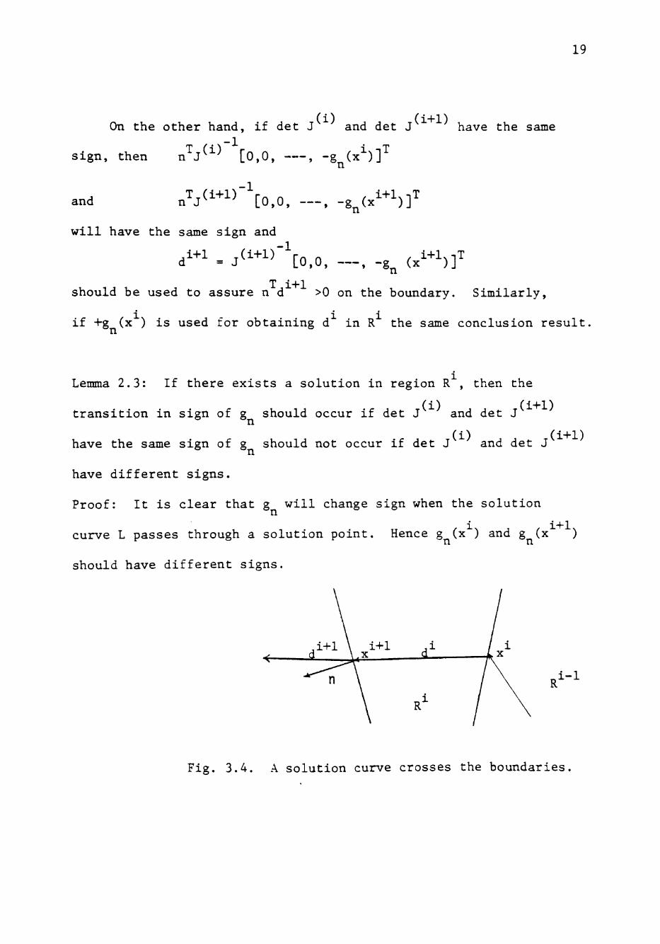
Lemma 2.3: If there exists a solution in region R , then the
transition in sign of g should occur if det J and det J o °n
have the same sign of g should not occur if det J and det J
have different signs.
Proof: It is clear that g will change sign when the solution
cuirve L passes through a solution point. Hence g (x ) and g (x )
should have different signs.
.i-1
Fig. 3.4. A solution curve crosses the boundaries.
Page 25
20
From the same argument as that given in Lemma 2., and
conditions
Tji - T^i _ n d >0, n d >0
.r.A A . ,{1) T Al)-1 . , .(i+l) T ^(i+l)-l and det J n J = det J n J ' ,
Lemma 2.3. is proved immediately.
In view of the above, the solution curve can easily be
taken care of at a local point on the boundary when Jacobian
determinants have arbitrary signs. Therefore the iterative
scheme of (3.15) allows continuation of tracing along the solution
curve L and, as a result, all the solutions on L can be obtained.
If g.(x) = 0,1,2, , n-1 defines a unique simple curve L,
that is, one with only a single branch, the L passes through
all the solutions of (3.14). Once a starting point on L is
obtained, all of the multiple solutions of (1.1) can be located
by using the technique described in this section. The following
lemma gives a sufficient condition for the existence and unique
ness of this solution curve.
Lemma 2.4: Let g(x) be a continuous piecewise-linear mapping of
R^ into itself and let J ^ denote the matrix by deleting the
kth row and nth column of Jacobian matrix J of region R , and
let J , denote the matrix consisting of the first m rows and km
first m columns of the constant Jacobian J, . If there exists
Page 26
a k, l<JiC^n, such that for each m = 1,2, , n-1, J, , J
21
km • "km ' ""' (N)
J j do not vanish and have the same sign then g.(x) = 0, j = 1,
2, , n-1 defines a unique simple curve.
Proof: Let h(x) = (g^(x), g2(x), , g _;L '' ^
and x_^ = (x^, x^, — , x^.i^x^+i. — , x^)^
If the value of x, is fixed, then the mapping h of R ~ into itself
is still a continuous piecewise-linear mapping. For any x, ,
h(x_ .,u) = \ x_^ + v^(u) - y_^, i = 1,2, , N
where y_^ = (y^.yj, — , yi . , 7^+1. — . y„)^
Since for each m, m = 1,2, , n-1, J, , , J, do not Icm Km
vanish and have the same sign, the mapping h with fixed x, is
a homeomophism of R onto itself. This implies that for any
given input y and any number u of x, there exists one and only
one point T
x_j (u) = (x^(u), X2(u), , X^_;L^^'^' ^+1^^-^' n - ^
such that h(x i,u) = 0. This guarantees the existence of a unique
continuous piecewise-linear function F: R ->R for h(x) = 0 such
that X ,= F(x, ). Hence F(x,) defines a unique simple curve L(x, )
in R for all
3.4 Starting Point
A starting point lying anywhere on the intersection L of
g.(x) = 0, i = 1,2, , n-1 has to be found before the root-finding
technique described in the previous section is applied.
Page 27
22 Let M be a positive number such that for any x » (x., x-,
T , X ) with X, >_ M, X is in an unbounded region. The union of
such unbounded regions is denoted by U. An arbitrary point x in
k k
R is chosen such that R U. With a fixed value of x, = u,
u >.M, a point x = Cx^(u), , Xj^_^(u), u, x^+^(u), , x^(u))^
which s a t i s f i e s g^(x) - 0, i » 1,2, , n-1 i s searched i n the (n-1) dimensional space R
Let g(x) be a continous p i e c e w i s e - l i n e a r mapping of R onto
i t s e l f defined i n ( 3 . 1 4 ) , and l e t J ^ ^ denote the matr ix by
d e l e t i n g the kth row and nth column of Jacobian mat r ix J of
the reg ion R .. In the following a lemma which was proved by
Kuh, Ohtsuki , and Fuijsawa Cl2] i s s t a t e d .
Lemma 2 . 5 . Let g be a continous p i e c e w i s e - l i n e a r mapping from
R i n t o i t s e l f defined by ( 3 . 1 4 ) . For an a r b i t r a r y v, i f det J
i = 1,2, ,N have same s i g n , then the re e x i s t s a t l e a s t one
s o l u t i o n X to the equat ion g(x) = 0. An immediate consequence of
Lemma 2.5 • i s as fo l lows.
Coro l l a ry : I f f o r a given k , 1 _<k<_ n , such t h a t in each region
R- , R" c ,^» ^ ]. <io ^ot vanish and have the same s ign then for
any x, , x, >^M, there e x i s t s a t l e a s t one s o l u t i o n for
g^(x) - 0 , i « 1, 2 , , n - 1 .
Page 28
23
This corollary gives a sufficient condition for the existence
of starting point x . The convergence to x from an arbitrary
initial guess in R-', R-'c U is guaranteed by the Katznelson's
algorithm.
3.5 Numerical Algorithm
The algorithm developed in previous section can be summarized
in the following steps.
Algorithm A:
Step 1. Find an initial point x in an unbounded region R according
to section 3.4. Set j = 0.
Step 2. Compute g(x ).
Step 3. If j=f 0, compute d according to Lemma 2. and Lemma 3.
^ 1- . ^0 .(O)"-'-, , 0, , 0.,T Otherwise, compute d = J ( -g,(x ) , - - - , -g (x )) .
i i i * Step 4. Compute x = x* + d . If x is in R then x = x is a
solution.
Step 5. Compute x-' = x" + X~ d , where X-" > 0 is the maximum value • • * * *
such that x(X) = x-"' + Xd" , 0 <_ X <_ X^ is in R^. If X^- » go
to step 7.
Step 6. Otherwise, identify region R-" . Set j = j +1 and go to
step 2.
Step 7. Set j = 0. Repeat step 2. to step 6. except in step 3. that
if j = 0 compute d° = J^°^ ( -g^{^^) . . +g^(x°))'^
gand in step 5. that if X-' ->•=», stop.
Two examples are given here for illustration,
Page 29
24
Example 3.1. Consider the nonlinear circuit of Fig. 3.5a, consisting
of two tunnel diodes and two constant current sources and a linear
resistor. The piecewise-linear approximation of function h for the
tunnel diode is given in Fig. 3.5b with
' 2x X < 3
h(x) -2.5ac + 13.5 3 < x < 5
1.5x-6.5 x > 5
Hence piecewise- l inear equations
8^^\x) J ^ ^ ^ + w^ - y 0, i - 1, 2, , 9
are obtained. All regions are shown in Fig. 3.6. The equation
associated with each region is given as:
g^»Cx) 3
1
3
1
1
3
^ r ^ 0
- 7
1
-1.5
X,
I 2
i
- y 13.5
S<^>(x)
3
1 2.5
/ \
-6.5 - 7
Ol li
S X, ©
Fig. 3.5a The circuit of example 3.1.
Page 30
25
g Cx) = -1.5 1
1 3
•\
.
f '
= 1
^2
+
f \
13.5
0 - y
8(^>(x) - 1 . 5
1
• 1
- 1 . 5
f >
\
""2
+
f \
13.5
13.5 - y
g^^) (X)
g"^x)
8^«>(x)
8^'^(x)
-1.5
1
2.5
1
2.5
1
2.5
1
1
2.5
1
3
• \
}
==1
^ J
+
'13.5'
-6.5 - y
^1
X, +
-6.5
0 - y
' 1
- 1 . 5
' -
"^x X
+
f ^
-6 .5
13.5 - y
1
2.5
^1
1= 2] +
-6 .5 '
-6 .5
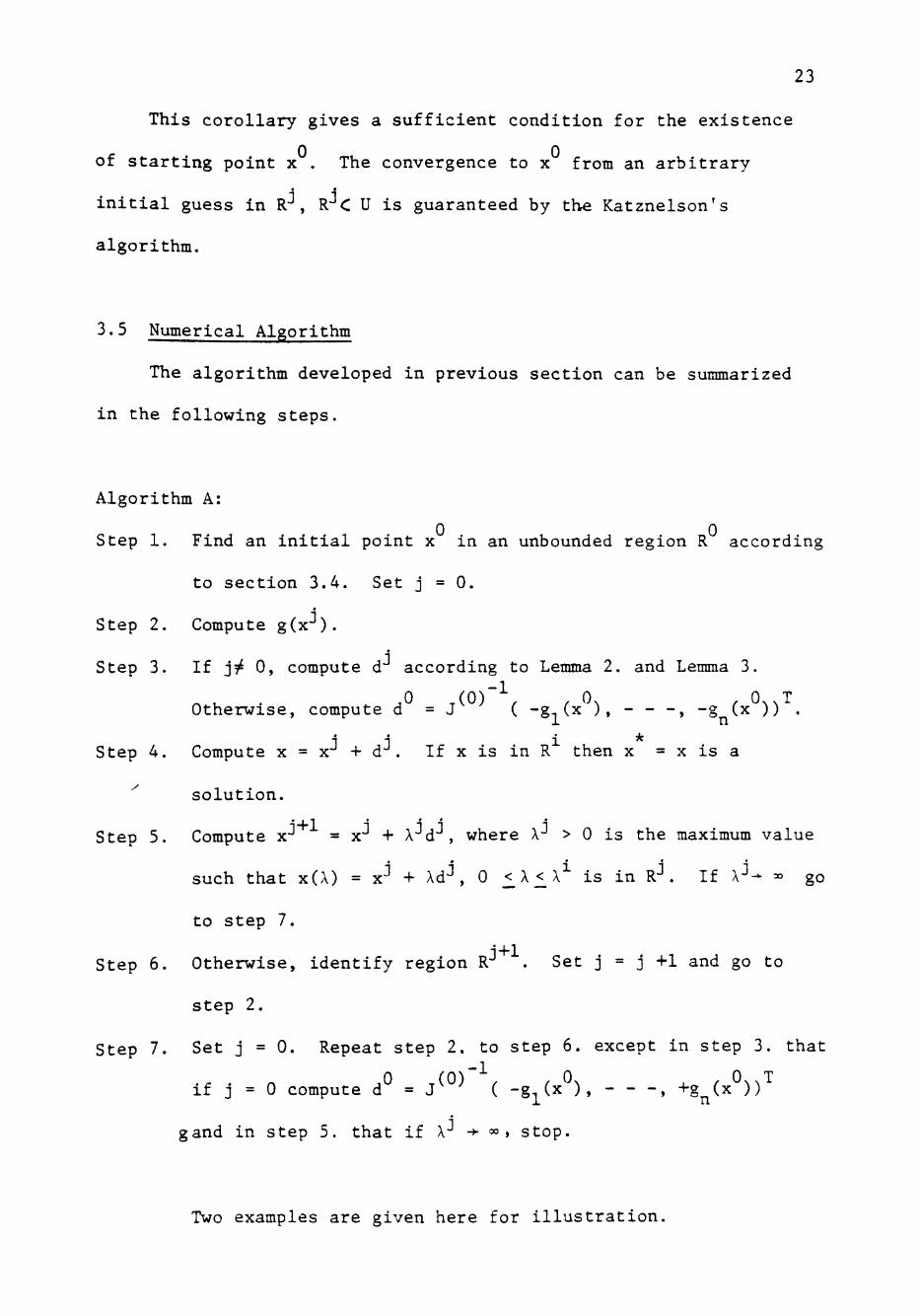
In this example, y, i.e. the input current source is given by
y =
13.5
13.5
h(x)i
3 5
Fig. 3.5b The piecewise-linear approximation of function
h for the tunnel diode
Page 31
26
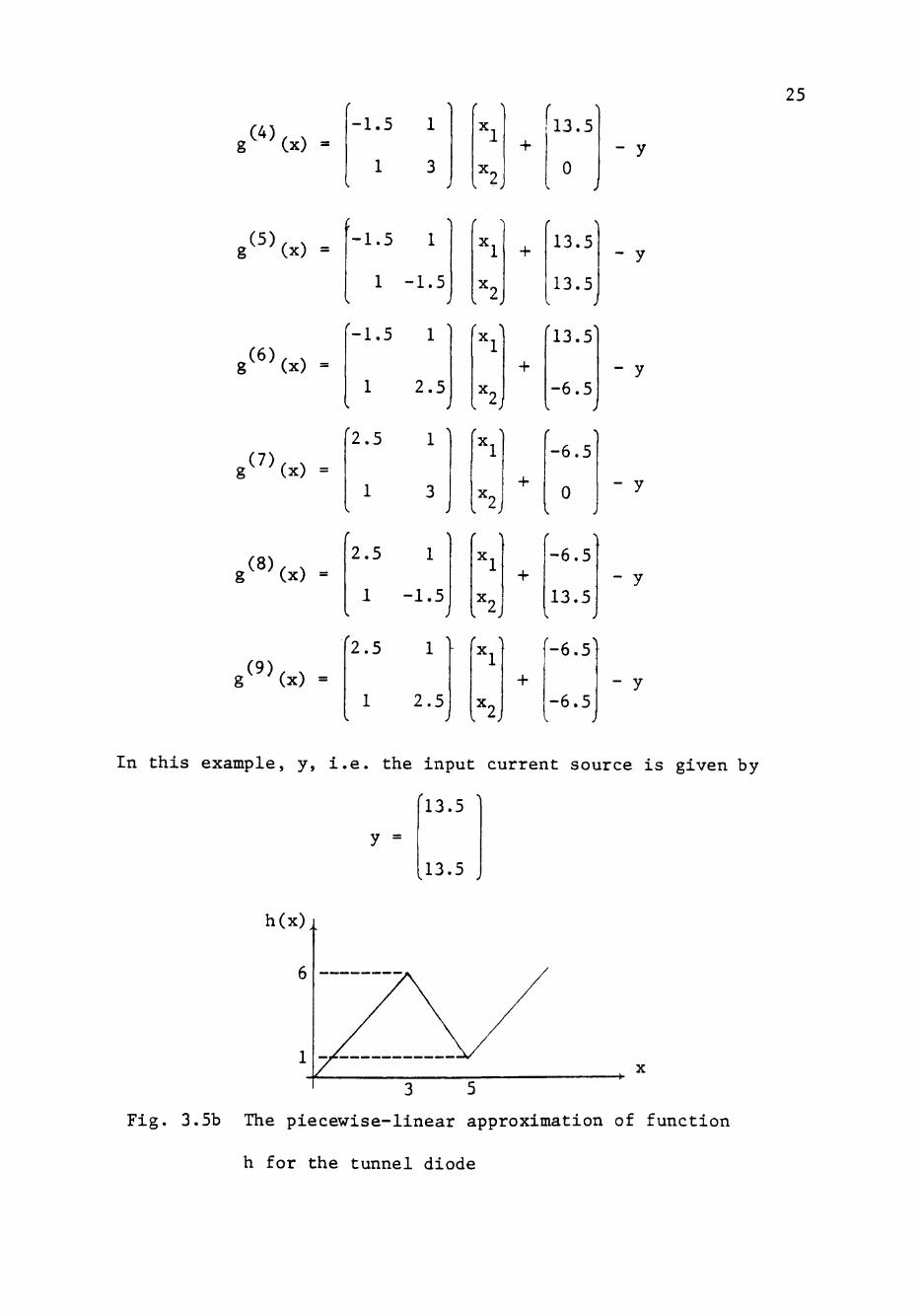
R3
R2
R1
R^
R5
R*
R '
R3
R^
X
Fig. 3.6. The regions in the x-space
If the solution curve L of g,»0 is traced, then the points
on L with g^» 0 are the desired solutions. For x.. >, 5, in each
7 8 9 unfaoxjnded region R , R , R oo"* 2.5 has the same sign and does
not vanish. Hence from Lemma 5, for a given value of x. = 5.5 > 5
0 T a corresponding solution x » Cy'5, 6.25) is found by solving
7 8 9 0
g_. Cxi = 0 in the unbounded regions R , R , R . Using x as a
starting point, the search along the curve L of g =0 leads to
five solutions C5.714, 5.714)^, (6.316, 4.211)^, (7.154, 2.115)*,
(4.211, 6.316)^, C2.115, 7..154) .
In fact, a simple solution curve does exist in this example
even though Lemma 4, is not satified. Similarly, if g O is
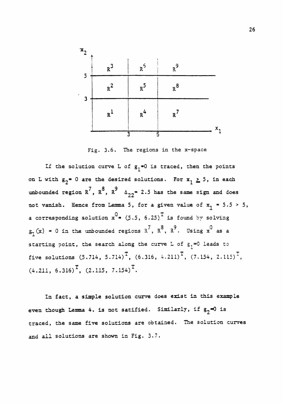
traced, the same five solutions are obtained. The solution curves
and all solutions are shown in Fig. 3.7.
Page 32
27
'0 .00 2.Do
ens
4.00 6.00 8.00 XI A X I S
IG.OO
F i g . 3 . 7 . So lu t ion curves of ejcample 3 .1
Page 33
28
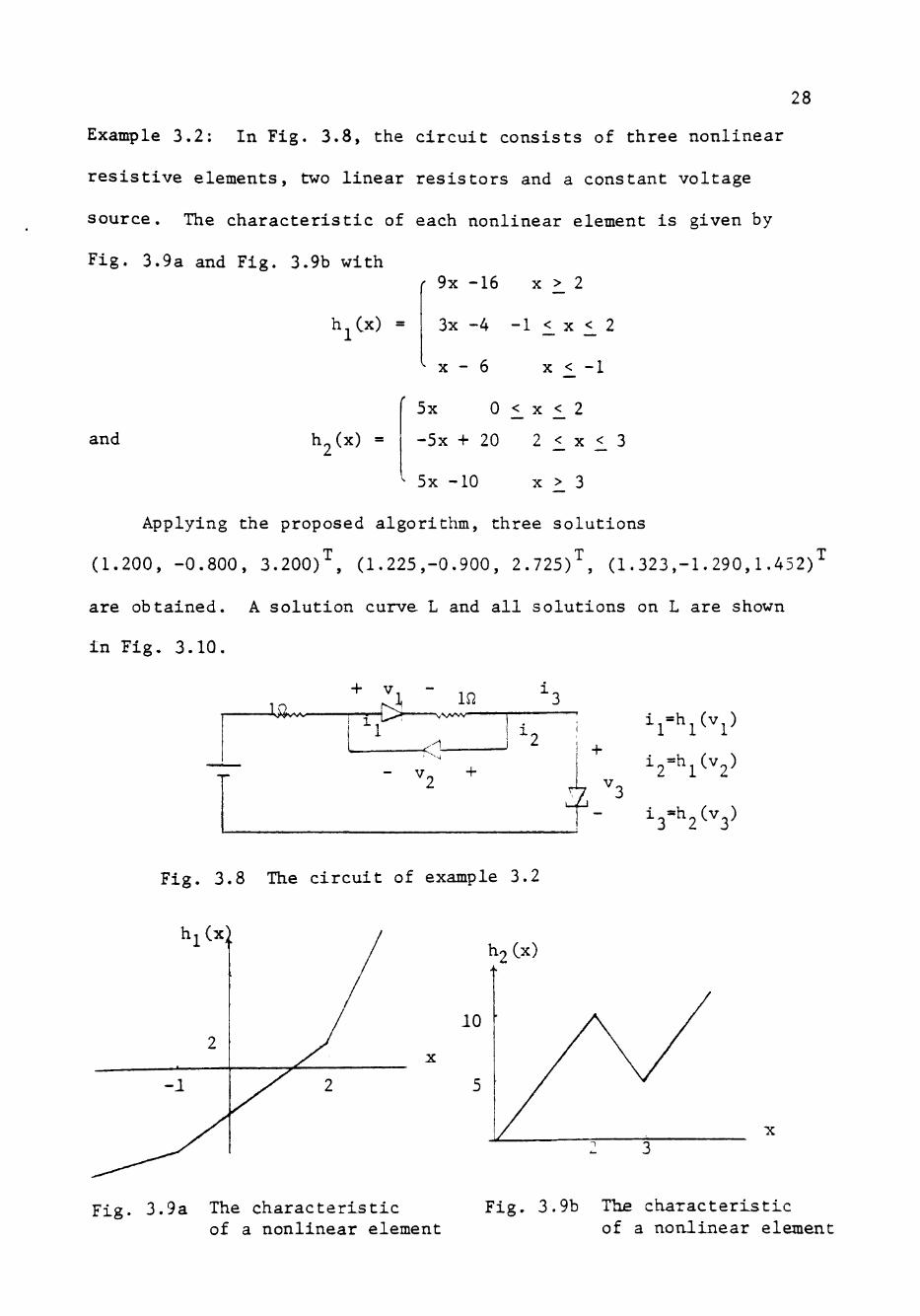
Example 3.2: In Fig. 3.8, the circuit consists of three nonlinear
resistive elements, two linear resistors and a constant voltage
source. The characteristic of each nonlinear element is given by
Fig. 3.9a and Fig. 3.9b with
h^Cx) =
9x -16 X > 2
3x -4 -1 1 X <_ 2
X - 6 X < -1
and h2(x) =
5x 0 <_ X <_ 2
-5x +20 2 < X < 3
5x -10 X > 3
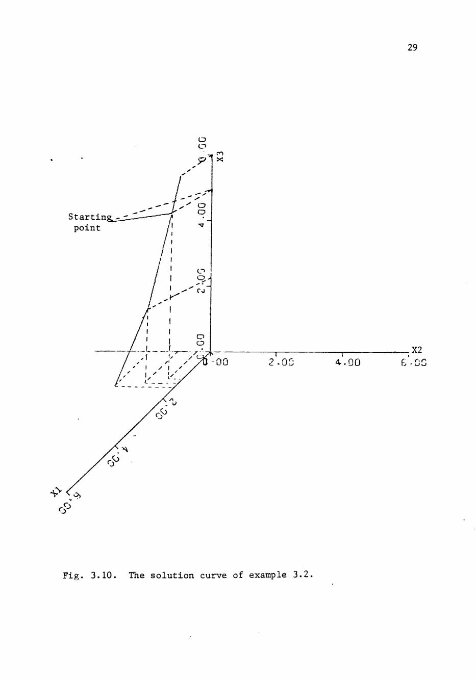
Applying the proposed algorithm, three solutions
(1.200, -0.800, 3.200)^, (1.225,-0.900, 2.725)^, (1.323,-1.290,1.452)-^
are obtained. A solution curve L and all solutions on L are shown
in Fig. 3.10.
—kWvw^ 10.
^A
- "2 ^
il=h^(vp
f- S=^2^^3^
Fig. 3.8 The circuit of example 3.2
hi(x) hoCx)
10
Fig. 3.9a The characteristic Fig. 3.9b The characteristic of a nonlinear element of a nonlinear element
Page 34
29
Startin point
2.00 4.Q0 X2
c r. o
<?
Fig. 3.10. The solution curve of example 3.2
Page 35
CHAPTER IV
CORNER PROBLEM AND THE PROBLEM OF
SINGULAR JACOBIAN MATRICES
^'1 The Corner Problem
This section is devoted to the study of the corner problem
[13, 16]. When a solution curve reaches a corner, the previous
algorithm cannot determine the next region which is to be entered.
Therefore, the proposed algorithm must be modified accordingly.
A boundary hyperplane in x-space can be represented by
I T ^ x ~ (x|nx = c } where n is the normal vector of the hyperplane
and c is a constant. A corner is a subset of the intersection
of two or more such hyperplanes. Since g = J x + w"*"- y
I T and H = { x | n x = c } , the image of any boundary hyperplane H
of region R is a hyperplane H in the g-space where
H = {g|Jj(i)"'g = c+nTj(^>'' (w^-y )}
Furthermore, the image of a corner in the x-space is a subset
of the intersection of two or more hyperplanes in the g-space.
Thus in the g-space HA.^^g|pg = q}= ^g|^-^ g=c+n J (w -y)}
where p is a nxl vector and q is a scalar, a corner can be
I T represented as a subset o f U = { g | P g = Q } where P is a (nx2)
matrix and Q is a (2x1) vector.
30
Page 36
31
Let
be a corner on the boundary of region R where P. and Q. are known
Since U is contained in Sp(U . ) , the linear manigold spanned by
U . which is an (n-1) dimensional subspace, there exists a (nxl)
unit vector h^ such that (h^) g =0 for all g U . . Let
i i 1 t>T,b, - - - b , constitute a basis for Sp (U . ) . Then h can 1 2 n-1 gi
be found by
(b , b^, , b^_^)V = 0 , (hS^ h = 1
where 0 is an (n-1) dimensional vector.
I T Thus, if a corner represented by U ,= {g| P. g=Q.} which is
on the boundary of region R is hit, then the solution line
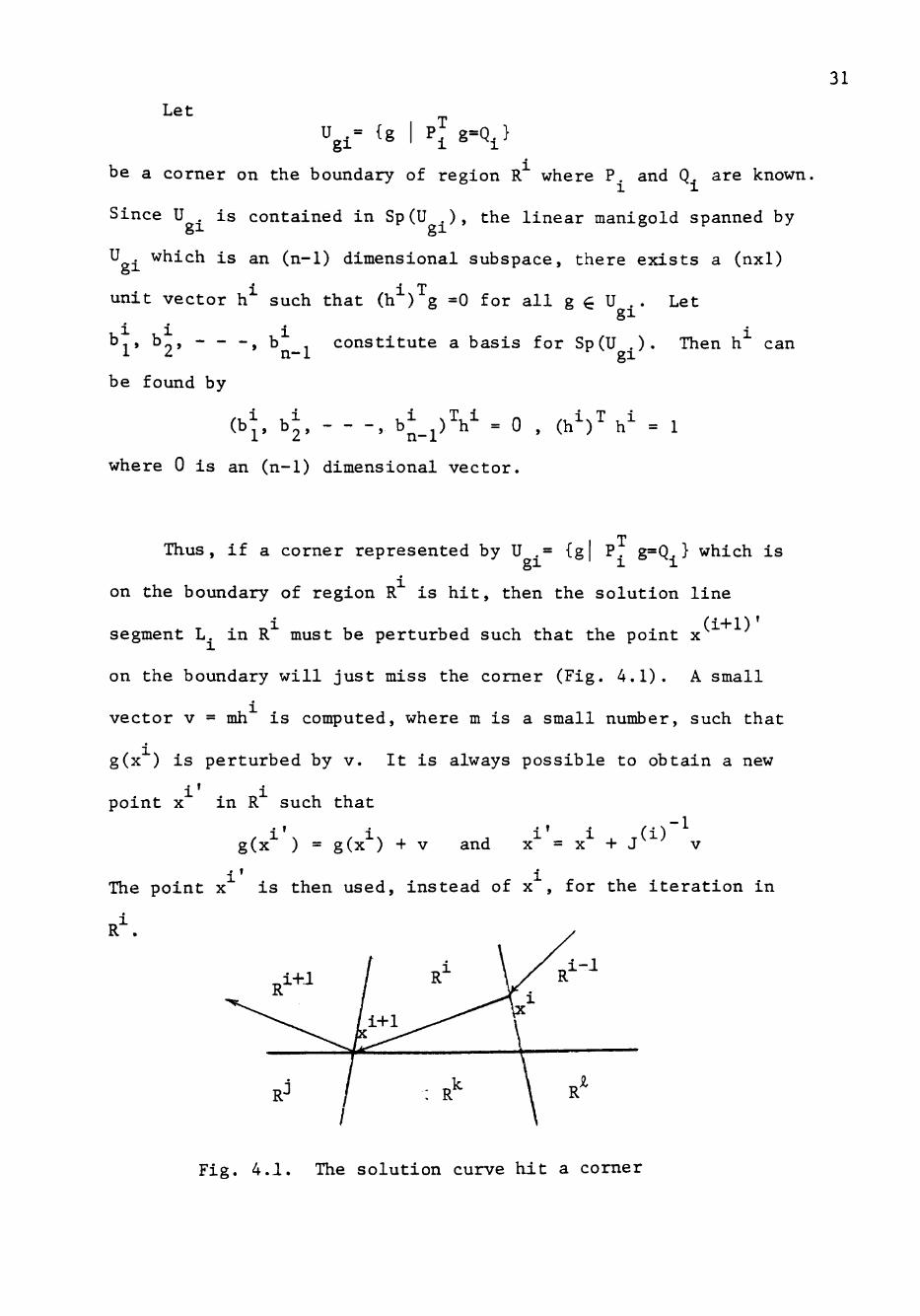
segment L. in R must be perturbed such that the point x
on the boundary will just miss the comer (Fig. 4.1). A small
vector V = mh is computed, where m is a small number, such that
g(x ) is perturbed by v. It is always possible to obtain a new
i i point X in R such that
g(x ) = g ( x ) + v and x = x + J v
i' i The point x is then used, instead of x , for the iteration in
R ^
Fig. 4.1. The solution curve hit a corner
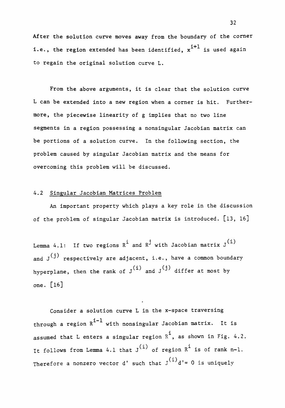
Page 37
32
After the solution curve moves away from the boundary of the comer
i.e., the region extended has been identified, x is used again
to regain the original solution curve L.
From the above arguments, it is clear that the solution curve
L can be extended into a new region when a corner is hit. Further
more, the piecewise linearity of g implies that no two line
segments in a region possessing a nonsingular Jacobian matrix can
be portions of a solution curve. In the following section, the
problem caused by singular Jacobian matrix and the means for
overcoming this problem will be discussed.
4.2 Singular Jacobian Matrices Problem
An important property which plays a key role in the discussion
of the problem of singular Jacobian matrix is introduced. [l3, 16]
Lemma 4.1: If two regions R and R^ with Jacobian matrix J
and J • respectively are adjacent, i.e., have a common boundary
hyperplane, then the rank of J and J -' differ at most by
one. [l6]
Consider a solution curve L in the x-space traversing
through a region R with nonsingular Jacobian matrix. It is
assumed that L enters a singular region R , as shown in Fig. 4.2
It follows from Lemma 4.1 that J of region R is of rank n-1.
Therefore a nonzero vector d' such that J d'= 0 is uniquely
Page 38
33
determined within constant multipliers. And the solution line
segment L. in R is obtained by
x(X) = x^ + Xd' where 0 <_ X ; X^
and X is determined such that x(X ) = x lies on another
hyperplane H. as indicated in Fig. 4.2 where H„ is between R
and R , By examining the mapping of L. into g-space, it is
found
g(x(X)) = J^^^x(X) + w" = J ' ( x^ + d') + w^
_(i) i , i , i. = J x + w =g(x)
i.e., the whole line segment L. is mapped into the single point
gCx ). Hence all the points on L. satify the Cn-1) equations
r \ n ' ^ o i T T j T i+l) 0 in the g.(x) = 0 , 1 = 1 , 2 , - - - , n-1. If det J
* I 1 * I 1
region of R in which x is lying, then according to Lemma 3.4
and Lemma 3.5, the solution curve can be extended into next region
R^+\ .i+1
In the special case when the next region R has also a
lingular Jacobian matrix, i.e., det J = 0 , then it follows
(i+l) from Lemma 4.1 that the rank of J is either n-1 or n-2
det J^^-^^^ 0
Fig. 4.2. The solution curve enters a singular region
Page 39
34
since J is of rank n-1. Suppose that J is of rank n-2,
then there exists a 2-dimensional plane S , containing x , such
2 i+1 2 that g(H2ns ) = { g (x )}. Since the hyperplane S H^ containing
X is at least one-dimensional, hence, if x' ? x is a point
9 ' .1.1
on S H^ then g(x') = g(x ). For two linearly independent
vectors (x'- x^) and (x " -x^), J^^\x'-x^) = J^^'^x^'^^-x^)
is satisfied in region R . Thus the rank of J is at most n-2,
which leads to a contradiction. Therefore the rank of J
must be n-1. The solution line segment L. .. can be extended
into region R from x by the same technique stated above,
and the singular Jacobian problem can thus be overcome.
Algorithm A can now be modified so that both the corner
problem and the problem of singular Jacobian problem are taken
care of. The new algorithm is summarized as follows.
Algorithm B:
Step 1. Use Algorithm A to trace the solution curve L.
Step 2. If a comer is hit by the solution curve L, then a
small vector v = mh is computed according to the
perturbation method stated in Section 4.1. A new point
i' i X is then computed and used, instead of x , to iterate
again in region R^. Once the solution curve move away
i+1 from the boundary of the corner, the point x on
the corner is used again to regain the solution curve.
Go to Step 1.
Page 40
35
Step 3. If a singular region R is identified by the present
solution curve L, then a vector d' is computed such that
J d' = 0 where J is the Jacobian matrix of region
R . Next iterative point x^ is determined by the
direction d'. Go to Step 1.
Page 41
CHAPTER V
APPLICATIONS
5.1 Piecewise-linear Analysis of AC Resistive Network
Resistive networks containing one or more time-varying
sources are known as as-resitive networks. In this case, the
network equation can be written in the form of
g(x(t), u(t)) = 0 (5.1)
where u(t) is the time varying input vector and x represents
the network variables. Thus, the operating point of the network
is a function of t. One way of solving (5.1) is to solve the
problem at different instants of time, which would be a time-
consuming practice. A continuation algorithm for finding the
solutions (5.1) for all t automatically has been proposed in [22],
Consider the differential equation
^ g(x(t), u(t)) = -g(x(t), u(t)) , g(x(tQ), u(tQ)) = 0
^ u(t) = w(t) , u(tQ) = u° (5.2)
where u is assumed to be continously differentiable and its
time derivative, w, is a known function of t. The initial
condition on g is such that s(t-.) = x is a solution of (5.1)
subject to u(tQ) = u . In the x-space, (5.2) is equvalent to
x = -J^^g(x, u) + | ^ w ) , x(tQ) = x° ^^'^^
36
Page 42
37
where J = r- . Thus, equation (5.3) can be integrated to fine x(t) d X
automatically.
The continuation algorithm -described above can be extended to
the case where g is a piecewise-linear function. Equation (5.3)
with a piecewise-linear g(x) can now be written as
-1
dt " ^^^^' "' ' au "'' ^^^0 47=-J^^^ (g(x, u) + | 4 w ) , x(tj = x° (5.4)
where J is the Jacobian matrix in the region R in which x
lies. Here it is assumed that J is nonsingular and u(t) is
a small signal vector such that x(t) will remain in R . As it
is noted that since J is a constant matrix, the solution x(t)
f ? can be represented as the superposition of two vectors x' and x
where x' is the solution of g(x, 0) = 0 and x'' is the response
only by the time-varying sources u(t). It is clear that x''(t)
possesses similar waveforms as u(t) since g(x, u) = 0 is a linear
function in region R .
If g(x, u ) = 0 has multiple solutions, then all the solution
points must be used as starting points of (5.4) in order to obtain
a complete family of solution curves. In the following example
a simple circuit is given to illustrate the approach just described,
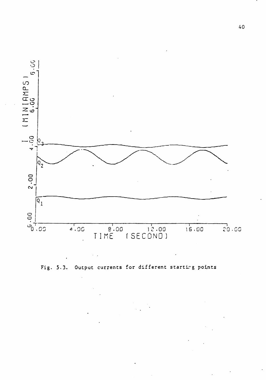
Example 5.1: Consider the nonlinear resistive circuit in Fig. 5.1
which consists of an ac source in series with a linear resistor
R = 600 ohm and a tunnel diode. The characteristic of the tunnel
Page 43
38
diode has been approximated by the following piecewise-linear
function.
i = h(v) =
r 0.006 V
0.024 - 0.006 V
V < 2
2 < V < 3
0.015 - 0.003 V 3 < V < 4
' 0.006 V - 0.021 V < 4
At t = 0, three operating points are first located by using the
method described in chapter III. The trajectories of v(t) and
i(t) for different Q points are plotted in Fig. 5.2 and Fig. 5.3
respectively.
If u(t) is large enough so that x(t) will not remain in the
region in which x(t-) lies, then the new region that x(t) will
enter must be identified and the Jacobian matrix in that region
should be substituted in (5.4). Proper J • ' s are switched back
and forth in (5.4) for different time intervals and the trajectory
for all t can be obtained accordingly.
600r i(t)
E ^ 6 . 2 volts
Qu(t)=0.3sint
; +
SL v(t)
Fig. 5.1. The circuit of example 5.1
Page 44
o t
39
o o
I
o o
CO
o o
O 'J cn
o o
O O
O O
0 .00 4 .00 8 . 0 0 12-00 TIME (SECOND)
16.00 2 0 . 0 0
Fig. 5.2. Output voltages for different starting points"
Page 45
40
LO CL
CTiD
:zui"
o o o. 0 .00 ^.OC 2 . 0 0 1 2 . 0 0 16 .00 2 0 . 0 0
T I M E ( S E C O N D ]
Fig. 5.3. Output currents for different startL- g points
Page 46
41
5.2 Dri-ving-Point or Transfer-Character is t ic Plots of
Multivalued Resistive Nonlinear Networks
Driving point plots and t ransfer cha rac te r i s t i c plots are
important in the analysis of nonlinear r e s i t ive networks because
they can pro-vide a deep insight to the nature of the c i r c u i t .
Bas ica l ly , the two concepts are the same; they are input-output
c h a r a c t e r i s t i c plots showing the relat ionship between a driving
source u. and a cer ta in output variable x . . Several methods 3 1
£18-20,23J are available for finding the input-output plots of
nonlinear r e s i t i v e networks.
Here the technique of continuation scheme for piecewise-linear
analysis of r e s i t i v e nonlinear networks developed in chapter I I I
i s applied to obtain the input-output p lo t s . The network equation,
in general , can be represented by
g(x, u) = 0 (5.6)
where g i s a continous piecewise-linear function, x i s an n-vector
of network va r i ab le s , and u denotes the m-vector of input source.
Since in finding input-output cha rac te r i s t i c plots a l l input
sources except one, say u. , are considered to be fixed, thus
(5.6) i s reduced to
g(x, u.) = 0. (5.7)
Suppose i t i s now required to find the input-output cha rac t e r i s t i c
. - + p lo t X versus u for u 1 u < u , Following the development
Page 47
42
given in [23], a set of (n+1) equations consisting of (5.7) and
an auxiliary equation g = 0 of the form
g(x, u.) = 0
Sn+l = j - = ° (5.8)
is considered. Application of the technique described in chapter
III, a continuous piecewise-linear curve L can be traced automatically
by the iterative scheme
i"» '' i+1^ X
i+1 u. "v J J
u
+ X' 3u,
0 l""
0
- 1 r -g(x^,uJ
t §n+l
(5.9)
g(x , u.) = 0
where J is the Jacobian matrix in the region of R and x is
the solution point of g(x, u,) = 0. The sign change should be
made when L traverses across a boundary and enters a new region
in which the determinant of the Jacobian matrix has a different
sign,
The advantage of this method is that the input-output plot is
not required to be either input or output controlled, i.e., the
plot may be obtained for multivalued networks. An example is
given in the following to illustrate the approach.
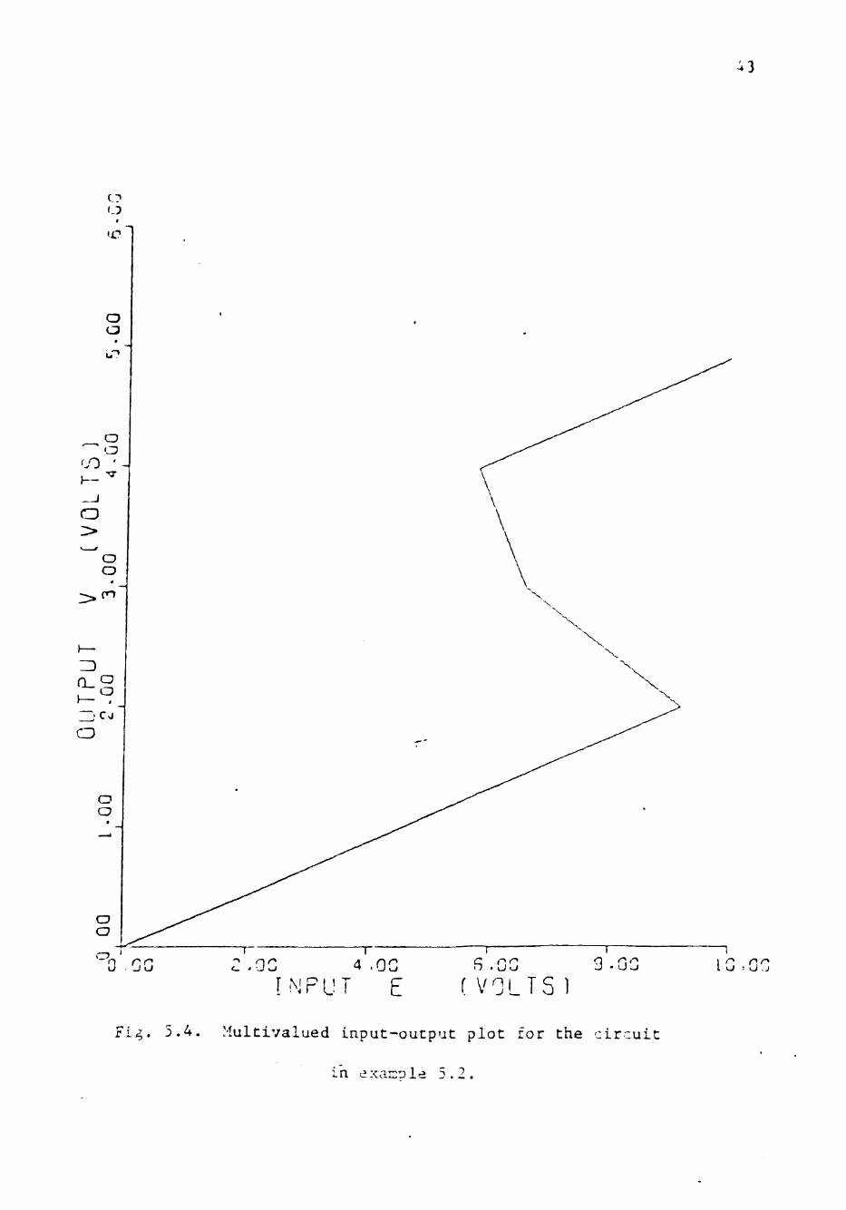
Example 5.2: Consider the tunnel diode problem studied in the
previous example. The input-output characteristic plots, v versus
E and i versus E, is graphed as the input E varies from 0 to 10
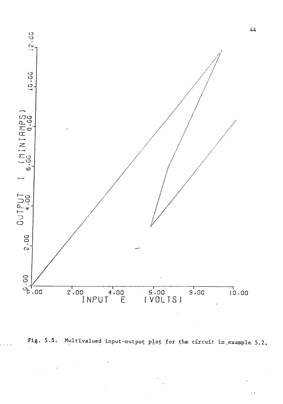
volts. The result is shown in Fig. 5.4 and Fig. 5,5.
Page 48
43
c?
[ N P U T E ( V O L T S ]
Fig . 5 .4 . Multivalued input -output p lo t for the c i r c u i t
.n exaiTDle 5 .2 .
Page 49
44
0 .00 2 . 0 0 4 .00 INPUT E
S--00 3 . 0 0 (VOLTS)
10=00
Fig . 5 . 5 . J^ultlvalued input-output p lo t for the. c i r cu i t Ln.esjample. 5.2^
Page 50
CHAPTER VI
CONCLUSION
In this report a systematic searching algorithm has been
presented for the piecewise-linear analysis of nonlinear resistive
networks. A set of continuous piecewise-linear equations g(x) = 0
is solved by tracing the solution curve L of any n-1 equations of
g(x) = 0 . As a result multiple solutions on L can be obtained.
Furthermore, a sufficient condition for the existence of a unique
simple curve L is given. It is clear that if L is simple, then all
the umltiple solutions of g(x) = 0 can be foimd by the proposed
search scheme.
In Chapter III, the local behavior of L on the boundary is
studied. A theory that guarantees the continuation of the search
algorithm when acrossing the boundary has developed. A method for
finding the starting point also been suggested. Methods for
overcoming the comer problem and singular Jacobian matrix problem
have been presented in Chapter IV. Applications to AC nonlinear
resitive network analysis and driving or transfer characteristic
curve of multivalued nonlinear network are given in Chapter V.
It is found that the algorithm developed here provides an efficient
and systematic way for solving the piecewise-linear nonlinear resis
tive network problems. However, if the solution curve consists of
multiple branches, only the solutions on the branch that contains
45
Page 51
46
the initial point can be found. A systematic method for locating
a starting point on every branch is worth of further research.
Page 52
LIST OF REFERENCES
[l] A. F. Malmberg, F. L. Comwell, and F. N. Hofer, "NET-1 network
analysis program", Los Alamos Sciences Lab., Rep. LA-3119, 7090/7094
version, August 1964.
[2] L. D. Milliman, W. A. Massena, and R. H. Dickhaut, "CTRCUS, A
digital computer program for transient analysis of electronic circuit
- user's g\iide", Harry Diamond Labs., The Boeing Co., Seattle, Wash.,
Rep. AD-364-1, January 1967.
[3] H. W. Mathers, S. R. Sedore, and J. R. Sents, "Automated digital
computer program for determining responses of electronic circuits
(SCEPTRE)", vol. 1, IBM Electronic System Center, Owego, N.Y., File
66-928-611, February, 1969.
[4] K. S. Chao, D. K. Liu, and C. T. Pan, "A systematic search method
for obtaining multiple solutions of simultaneous nonlinear equations",
IEEE Trans. Circuits Syst,, vol. CAS-22, pp. 748-753, Sept. 1975.
[5] F. H. Branin, Jr., "Widely convergent method for finding multiple
solutions of simultaneous nonlinear equations", IBM J. Res. Develop.,
vol. 16, no. 5, pp. 506-522, Sept. 1972.
[6] L. 0. Chua and A. Ushida, "A switching-parameter algorithm for
finding multiple solutions of nonlinear resitive circuits". Int. J.
Circuit Theory and Applications, vol. 4, no. 3, pp. 215-239, July 1976.
[7] R. P. Brent, "On the Davidento-Branin method for solving simu
ltaneous nonlinear equations", IBM J. Res. Develop., vol. 16, no. 4,
pp. 434-436, July 1972.
47
Page 53
ar
48
Lsj E. S. Kuh and I. N. Hajj, "Nonlinear circuit theory: Resistive
networks", Proc. IEEE, vol. 59, pp. 340-355, March 1971.
19J C. T. Pan, "A discrete approach for solving nonlinear equations"
Master's thesis, Texas Tech University, 1974.
ilQj J. Katznelson, "An algorithm for sol-ving nonlinear resistive
networks" Bell System Tech. J. vol. 44, pp. 1605-1620, 1965.
[ll] T. Fujjsawa and E. S. Kuh, "Piecewise-linear theory of nonline
networks", SIAM J. Appl. Math. vol. 22, pp. 307-328, 1972.
[12] T. Ohtsuki, T. Fujjsawa, and E. S. Kuh, "A sparse matrix method
for analysis of piecewise-linear resistive networks", IEEE Trans.
Circuit Theory, CT-19, pp. 571-584, 1972.
[13] M. J. Chien and E. S. Kuh, "Solving piecewise-linear equations
for resistive networks". Int. J. Circuit Theory and Appl., vol. 4,
no. 1, pp. 3-24, January 1976.
[14J M. J. Chien and E. S. Kuh, "Solving nonlinear resistive networks
using piecewi e-linear analysis and simplicial subdivision", IEEE
Trans. Circuits Syst., vol. CAS-24, no. 6, pp. 305-317, June 1977.
[15] L. 0. Chua, "Efficient computer algorithm for piecewise-linear
analysis of resistive nonlinear networks", IEEE Trans. Circuits
Theory, vol. CT-18, pp. 73-85, January 1971.
[I6] T. Ohtsuki, T. Fujjsawa and S. Kumagai, "Existence theorems
and a solution algorithm for piecewise-linear resistive networks",
SIAM J. Appl. Math. 1977.
I17] H. C. So, "On the hybrid description of a linear n-port result
ing from the extraction of arbitrarily specified elements", IEEE Trans
Page 54
49
[18] L. 0. Chua, Introduction to Nonlinear Network Theory, McGraw-
Hill, New York, N.Y., 1969.
[19J G. H. Meyer, "On Solving nonlinear equations with a one-parameter
operator imbedding", SIAM J. Numer. Analy., vol. 5, pp. 739-752, 1968.
[20] V. C. Prasad and A. Prabhakar, "Input-output plots of piecewise-
linear resistive networks", Proc. 1974 IEEE Int. Symp. Circuits and
Systems, April 1974, pp. 55-59.
12l] R. Saeks and R. A. Decarlo, Interconnected Dynamical Systems,
New York, Marcel Dekker (to appear).
[22] C. T. Pan, "Integration Methods in System Analysis", PH.D.
dissertation, Texas Tech University, 1976.
[23] K. S. Chao and R. Saeks, "Continuation Methods in Circuit
Analysis", Proc. IEEE, vol. 65, no. 8, August 1977.