UCRL-CONF-211357

A Contract Based System ForLarge Data Visualization

H. R. Childs, E. S. Brugger, K. S. Bonnell, J. S.Meredith, M. C. Miller, B. J. Whitlock, N. L. Max

April 14, 2005

A Contract Based System For Large Data VisualizationMinneapolis, MN, United StatesOctober 23, 2005 through October 28, 2005

Disclaimer

This document was prepared as an account of work sponsored by an agency of the United States Government. Neither the United States Government nor the University of California nor any of their employees, makes any warranty, express or implied, or assumes any legal liability or responsibility for the accuracy, completeness, or usefulness of any information, apparatus, product, or process disclosed, or represents that its use would not infringe privately owned rights. Reference herein to any specific commercial product, process, or service by trade name, trademark, manufacturer, or otherwise, does not necessarily constitute or imply its endorsement, recommendation, or favoring by the United States Government or the University of California. The views and opinions of authors expressed herein do not necessarily state or reflect those of the United States Government or the University of California, and shall not be used for advertising or product endorsement purposes.

A Contract Based System For Large Data Visualization ∗

Hank Childs†

University of California, Davis/Lawrence Livermore National Laboratory

Eric Brugger, Kathleen Bonnell, Jeremy Meredith, Mark Miller, and Brad Whitlock ‡

Lawrence Livermore National Laboratory

Nelson Max§

University of California, Davis

ABSTRACT

VisIt is a richly featured visualization tool that is used to visual-ize some of the largest simulations ever run. The scale of thesesimulations requires that optimizations are incorporated into everyoperation VisIt performs. But the set of applicable optimizationsthat VisIt can perform is dependent on the types of operations be-ing done. Complicating the issue, VisIt has a plugin capability thatallows new, unforeseen components to be added, making it evenharder to determine which optimizations can be applied.

We introduce the concept of a contract to the standard data flownetwork design. This contract enables each component of the dataflow network to modify the set of optimizations used. In addition,the contract allows for new components to be accommodated grace-fully within VisIt’s data flow network system.

Keywords: large data set visualization, data flow networks,contract-based system

1 INTRODUCTION

VisIt is an end-user visualization and data analysis tool for diversedata sets, designed to handle data sets from thousands to millionsto billions of elements in a single time step. The tool has a richfeature set; there are many options to subset, transform, render, andquery data. VisIt has a distributed design. A server utilizes parallelcompute resources for data reduction, while a client runs on a localdesktop machine to maintain interactivity. The rendering primitivesresulting from the data reduction phase are typically transferred tothe client and rendered using graphics hardware. When the numberof primitives overwhelms the client, the geometry is kept on theserver and rendered using a sort-last rendering technique [9]. VisIt’srendering phase is outside the scope of this paper. Instead, we willfocus on the data reduction phase and the optimizations necessaryto handle large data sets.

VisIt employs a modified data flow network design [13] [1] [11].Its base types are data objects and components (sometimes calledprocess objects). The components can be filters, sources, or sinks.Filters have an input and an output, both of which are data objects.Sources have only data object outputs and sinks have only data ob-ject inputs. A pipeline is a collection of components. It has a source(typically a file reader) followed by many filters followed by a sink(typically a rendering engine). Pipeline execution is demand driven,meaning that data flow starts with a pull operation. This beginsat the sink, which generates an update request that propagates upthe pipeline through the filters, ultimately going to a load balancer(needed to divide the work on the server) and then to the source.

∗This is LLNL Report UCRL-CONF-211357.†e-mail: childs3@llnl.gov‡e-mail: {brugger1,bonnell2,meredith6,miller86,whitlock2}@llnl.gov§e-mail: max@cs.ucdavis.edu

The source generates the requested data which becomes input tothe first filter. Then execute phases propagate down the pipeline.Each component takes the data arriving at its input, performs someoperation and creates new data at its output until the sink is reached.These operations are typical of data flow networks. VisIt’s data flownetwork design, is unique, however, in that it also includes a con-tract which travels up the pipeline along with update requests (seeFigure 1).

Figure 1: An example pipeline.During the update phase (de-noted by thin arrows), ContractVersion 0 (V0), comes from thesink. V0 is then an input tothe contour filter, which modifiesthe contract to make ContractVersion 1 (V1). This continuesup the pipeline, until an execu-tive that contains a load balancer(denoted by LB) is reached. Thisexecutive decides the details ofthe execution phase and passesthose details to the source, whichbegins the execute phase (de-noted by thick arrows).

VisIt is a large and complex system. It contains over 400 differ-ent types of components and data objects. It has over one millionlines of source code and depends on many third party libraries. Inaddition, VisIt has a plugin capability that allows users to extendthe tool with their own sources, sinks, filters, and even data objects.

The scale of the data sets processed by VisIt mandates that op-timizations are incorporated into every pipeline execution. Theseoptimizations vary from minimizing the data read in off disk to thetreatment of that data to the way that data moves through a pipeline.The set of applicable optimizations is dependent on the propertiesof the pipeline components. This requires a dynamic system thatdetermines which optimizations can be applied. Further, becauseof VisIt’s plugin architecture, this system must be able to handlethe addition of new, unforeseen components. VisIt’s strategy is tohave all of a pipeline’s components modify a contract and have op-timizations adaptively employed based on the specifications of thiscontract.

The heart of VisIt’s contract-based system is an interface thatallows pipeline components to communicate with other filters anddescribe their impact on a pipeline. Focusing on the more abstractnotion of impact rather than the specifics of individual componentsallows VisIt to be a highly extensible architecture, because newcomponents simply must be able to describe what impacts they willhave. This abstraction also allows for effective management of thelarge number of existing components.

Because the contract is coupled with update requests, the infor-mation in the contract travels from the bottom of the pipeline to thetop. When visiting each component in the pipeline, the contract

is able to inform that component of the downstream components’requirements, as well as being able to guarantee that the compo-nents upstream will receive the current component’s requirements.Further, the contract-based system enables all components to par-ticipate in the process of adaptively selecting and employing appro-priate optimizations. Finally, combining the contract with updaterequests has allowed for seamless integration into VisIt.

2 BACKGROUND

2.1 Description of Input Data

Most of the data sets processed by VisIt come from parallelizedsimulation codes. In order to run in parallel, these codes decomposetheir data into pieces, called domains. The domain decompositionis chosen so that the total surface area of the boundaries betweendomains is minimized, and there is typically one domain for eachprocessor. Also, when these codes write their data to disk, it istypically written in its domain decomposed form. Reading in onedomain from these files is usually an atomic operation; the data islaid out such that either it is not possible or it is not advantageousto read in a portion of the domain.

Some data sets provide meta-data to VisIt, allowing VisIt tospeed up their processing. We define meta-data to be data aboutthe data set that is much smaller in size than the whole data set.Examples of meta-data are spatial extents for each domain of thesimulation or variable extents for each domain for a specific vari-able of the simulation.

VisIt leverages the domain decomposition of the simulation forits own parallelization model. The number of processors that VisIt’sparallel server is run on is typically much less than the number ofdomains the simulation code produced. So VisIt must support do-main overloading, where multiple domains are processed on eachprocessor of VisIt’s server. Note that it is not sufficient to simplycombine unrelated domains into one larger domain. This is not evenpossible for some grid types, like rectilinear grids where two gridsare likely not neighboring and cannot be combined. And for situa-tions where grids can be combined, like with unstructured grids, ad-ditional overhead would be incurred to distinguish which domainsthe elements in the combined grid originated from, which is impor-tant for operations where users want to refer to their elements intheir original form (for example, picking elements).

The simulation data VisIt handles is some of the biggest everproduced. For example, VisIt was recently used to interactivelyvisualize a data set comprised of 12.7 billion elements per time stepusing only eighty processors. In addition, there are typically on theorder of one thousand time steps for each simulation. The grids areunstructured, structured, or rectilinear. There are also scattered dataand structured Adaptive Mesh Refinement (AMR) grids.

2.2 Related Work

VisIt’s base data flow network system is similar to those im-plemented in many other systems, for example VTK [11],OpenDX [1], and AVS [13]. The distinguishing feature of VisIt’sdata flow networks is the contract that enables optimizations to beapplied adaptively. It should be noted that VisIt makes heavy useof VTK [6] modules to perform certain operations. Many of VisIt’sdata flow network components satisfy their execute phase by of-floading work to VTK modules. But VisIt’s abstract data flow net-work components remain distinct from VTK and, moreover, haveno knowledge of VTK.

There are several other richly-featured parallel visualizationtools that perform data reduction in parallel followed by a combinedrendering stage, although these tools frequently do not support op-erating on the data in its original form (including domain overload-

ing) in conjunction with collective communication. Examples ofthese are EnSight [4], ParaView [7], PV3 [5] and FieldView [8].

The concept of reading in only chunks of a larger data set (SeeSection 3.1) has been well discussed, for example by Chiang, etal. [3] and Pascucci et al. [10]. But these approaches typically donot support operating on the data in its native, domain decomposedform nor operating at the granularity of its atomic read operations(i.e. domains).

One of VisIt’s execution models, called streaming (See Section3.2), maps well to out-of-core processing. Many out-of-core al-gorithms are summarized by Silva et al. [12]. In addition, Ahrenset al. [2] gives an overview of a parallel streaming architecture. Itshould be noted that VisIt’s streaming is restricted to domain granu-larity, while the system described by Ahrens allows for finer granu-larity. In this paper, the discussion will be limited to deciding whenstreaming is a viable technique and how the contract-based systemenables VisIt to automatically choose the best execution model fora given pipeline.

Ghost elements are typically created by the simulation code andstored with the rest of the data. The advantages of utilizing ghostelements to avoid artifacts at domain boundaries (See Section 3.3)were discussed in [2]. In this paper, we propose that the post-processing tool (e.g. VisIt) be used to generate ghost data whenghost data is not available in the input data. Further, we discussthe factors that require when and what type of ghost data shouldbe generated, as well as a system that can incorporate these factors(i.e. contracts).

3 OPTIMIZATIONS

In the following sections, some of the optimizations employed byVisIt will be described. The potential application of these optimiza-tions is dependent on the properties of a pipeline’s components.VisIt’s contract-based system is necessary to facilitate these opti-mizations being applied adaptively.

After the optimizations are described, a complete description ofVisIt’s contract-based system will be presented.

3.1 Reading the Optimal Subset of Data

I/O is the most expensive portion of a pipeline execution for almostevery operation VisIt performs. VisIt is able to reduce the amount oftime spent in I/O to a minimum by reading only the domains that arerelevant to any given pipeline. This performance gain propagatesthrough the pipeline, since the domains not read in do not have tobe processed downstream.

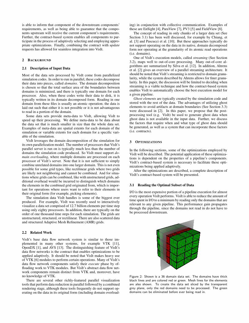
Figure 2: Shown is a 36 domain data set. The domains have thickblack lines and are colored red or green. Mesh lines for the elementsare also shown. To create the data set sliced by the transparentgrey plane, only the red domains need to be processed. The greendomains can be eliminated before ever being read in.

Consider the example of slicing a three-dimensional data set bya plane (see Figure 2). Many of the domains will not intersect theplane and reading them in will be wasted effort. In fact, the numberof domains (D) that are intersected by the slice is typically O(D2/3).

With the presence of meta-data, it is possible to eliminate do-mains from processing before ever reading them. For example, ifthe slice filter had access to the spatial extents for each domain, itcould calculate the list of domains whose bounding boxes intersectsthe slice and only process that list (note that false positives can po-tentially be generated by considering only the bounding box).

VisIt’s contract methodology enables this. During the updatephase, every filter is given an opportunity to modify the contract,which contains the list of domains to be processed. A filter cancheck to see if some piece of meta-data is available (for example,spatial extents), and, if so, cross-reference the list of domains tobe processed with the meta-data. The modified contract will thencontain only those domains indicated by the filter.

It is important to note that every filter in the pipeline has a chanceto modify the contract. If a pipeline had a slice filter and a contourfilter (to generate isolines), the slice filter could use a spatial extentsmeta-data object to get exactly the set of domains that intersectedthe slice, while the contour filter could use a data extents meta-dataobject to get exactly the set of domains that could possibly producecontours. The resulting contract would contain the intersection oftheir two domain lists.

Further, since the infrastructure for subsetting the data is encap-sulated in the contract, plugin filters can leverage this optimization.For example, a plugin spherical-slice filter can be added afterwardsand it can also make use of the spatial extents meta-data, or a pluginfilter that thresholds the data to produce only the elements that meeta certain criteria (elements with density between 2 g/cc and 5 g/cc,for example) can use the data extents meta-data. Also, the types ofmeta-data incorporated are not limited to spatial and data extents.They can take any form and can be arbitrarily added by new plugindevelopers.

3.2 Execution Model

VisIt has two techniques to do domain overloading. One approach,called streaming, will process domains one at a time. In this ap-proach, there is one pipeline execution for each domain. Anotherapproach, called grouping, is to execute the pipeline only once andto have each component process all of the domains before proceed-ing to the next one.

VisIt can employ either streaming or grouping when doing itsload balancing. With static load balancing, domains are assignedto the processors at the beginning of the pipeline execution and agrouping strategy is applied. Because all of the data is availableat every stage of the pipeline, collective communication can takeplace, enabling algorithms that cannot be efficiently implementedin an out-of-core setting. With dynamic load balancing, domainsare assigned dynamically and a streaming strategy is applied. Notall domains take the same amount of time to process; dynamic loadbalancing efficiently (and dynamically) schedules these domains,creating an evenly distributed load. In addition, this strategy willprocess one domain in entirety before moving on to the next one,increasing cache coherency. However, because the data streamsthrough the pipeline, it is not all available at one time and collectivecommunication cannot take place with dynamic load balancing.

So how does VisIt decide which load balancing method to use?Dynamic load balancing is more efficient when the amount of workper domain varies greatly, but the technique does not support allalgorithms. Static load balancing is usually less efficient, but doessupport all algorithms. The best solution is to use dynamic load bal-ancing when possible, but fall back on static load balancing whenan algorithm can not be implemented in a streaming setting. VisIt’s

contract system is again used to solve this problem. When eachpipeline component gets the opportunity to modify the contract, itcan specify whether or not it will use collective communication.When the load balancer executes, it will consult the contract andthen use that information to adaptively choose between dynamicand static load balancing.

3.3 Generation of Ghost Data

Although handling the data set as individual domains is a goodstrategy, problems can arise along the exterior layer of elementsof a domain that would not occur if the data set was processed as asingle, monolithic domain.

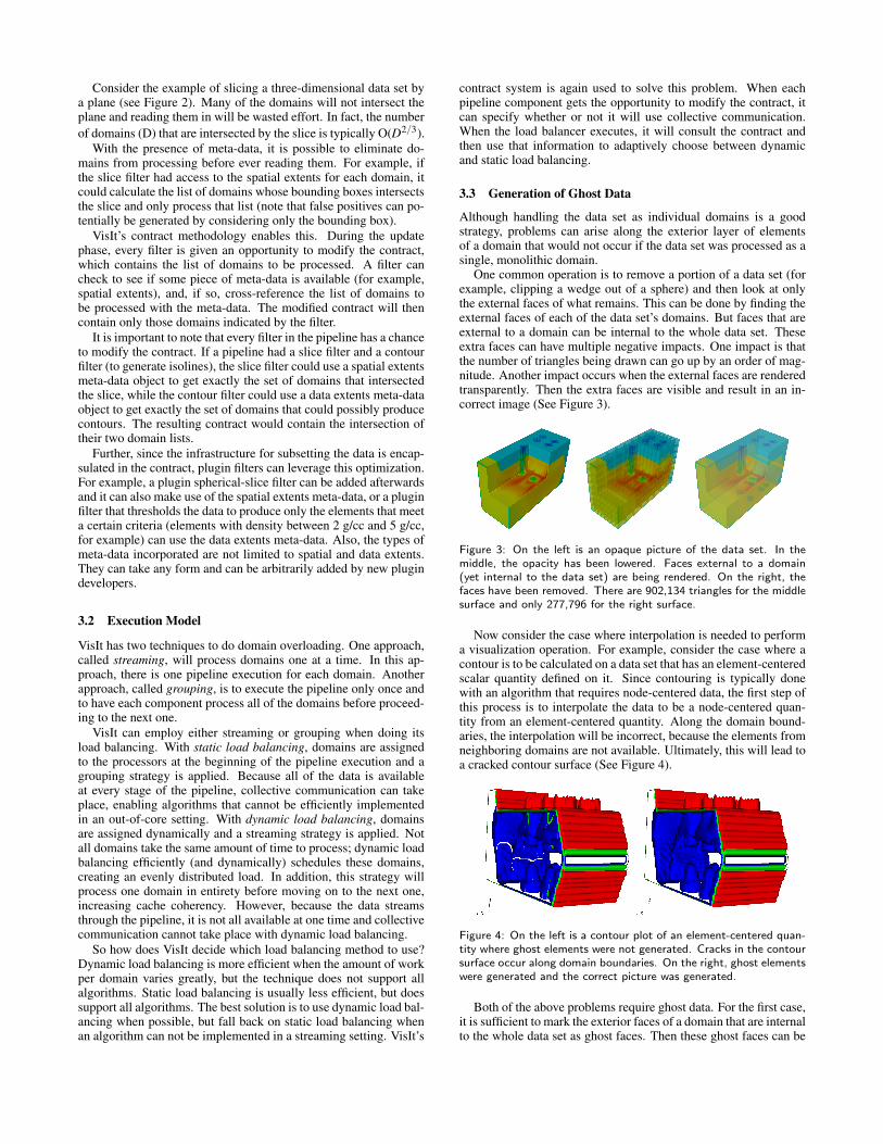
One common operation is to remove a portion of a data set (forexample, clipping a wedge out of a sphere) and then look at onlythe external faces of what remains. This can be done by finding theexternal faces of each of the data set’s domains. But faces that areexternal to a domain can be internal to the whole data set. Theseextra faces can have multiple negative impacts. One impact is thatthe number of triangles being drawn can go up by an order of mag-nitude. Another impact occurs when the external faces are renderedtransparently. Then the extra faces are visible and result in an in-correct image (See Figure 3).

Figure 3: On the left is an opaque picture of the data set. In themiddle, the opacity has been lowered. Faces external to a domain(yet internal to the data set) are being rendered. On the right, thefaces have been removed. There are 902,134 triangles for the middlesurface and only 277,796 for the right surface.

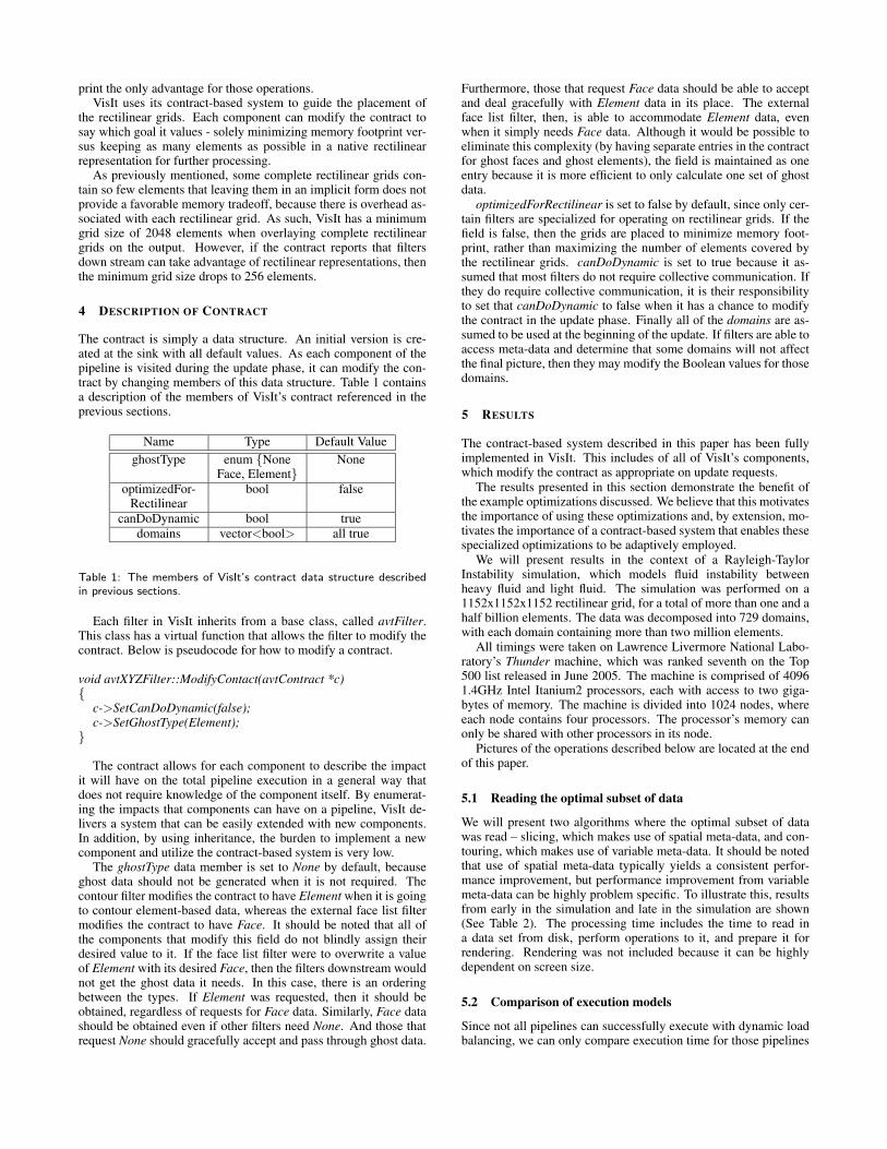
Now consider the case where interpolation is needed to performa visualization operation. For example, consider the case where acontour is to be calculated on a data set that has an element-centeredscalar quantity defined on it. Since contouring is typically donewith an algorithm that requires node-centered data, the first step ofthis process is to interpolate the data to be a node-centered quan-tity from an element-centered quantity. Along the domain bound-aries, the interpolation will be incorrect, because the elements fromneighboring domains are not available. Ultimately, this will lead toa cracked contour surface (See Figure 4).

Figure 4: On the left is a contour plot of an element-centered quan-tity where ghost elements were not generated. Cracks in the contoursurface occur along domain boundaries. On the right, ghost elementswere generated and the correct picture was generated.

Both of the above problems require ghost data. For the first case,it is sufficient to mark the exterior faces of a domain that are internalto the whole data set as ghost faces. Then these ghost faces can be

discarded when an external face list is generated. The second caserequires a redundant layer of ghost elements around the exterior ofeach domain. This allows interpolation to be done correctly.

Generation of ghost data is typically possible given some de-scription of the input data set. This input can take several forms.One form can be a description of how the domain boundaries ofstructured meshes overlap (”faces I=0-5, J=0, K=8-12 of domain5 are the same as faces I=12-17, J=17, K=10-14 of domain 12”).Another form utilizes global node identifiers assigned by the simu-lation code for each node in the problem. The visualization tool canthen use these identifiers to determine which nodes are duplicatedon multiple domains and thus identify shared boundaries betweendomains, which is the key step for creating ghost data. A third formuses the spatial coordinates of each node as a surrogate for globalnode identifiers. For each of these forms, the salient issue is thata module can be written where VisIt can give the module the in-put data and request it to create ghost faces or ghost elements. Thedetails of such a module are not important to this paper.

There are costs associated with ghost data. Routines to generateghost elements are typically implemented with collective commu-nication, which precludes dynamic load balancing. In addition,ghost elements require a separate copy of the data set (see Figure5), increasing memory costs. Ghost faces are less costly, but stillrequire arrays of problem size data to track which faces are ghostand which are not. To this end, it is important to determine theexact type of ghost data needed, if any.

Figure 5: On the left is a domain without ghost elements. On theright is the same domain with ghost elements added (drawn in yel-low). VisIt combines the ghost elements with the domain’s real el-ements into one large domain for efficiency purposes for the filtersdownstream as well as simplicity of coding.

VisIt’s contract system ensures that the minimum calculation isperformed. If a filter, such as the contour filter, needs to do interpo-lation, it will mark the contract with this information on the updatephase. As a result, ghost elements will be created at the top of thepipeline, allowing correct interpolation to occur. If the filter be-lieves it will have to calculate external face lists, the case with theexternal face list filter, then it will mark the contract with this infor-mation on the update phase, and ghost faces will be created. Mostimportantly, in cases that do not require ghost data, such as the casewhen a data set is being sliced or volume rendered, no ghost datawill be created.

3.4 Subgrid Generation

Before discussing subgrid generation, first consider VisIt’s Clip andThreshold filters. Clipping allows a user to remove portions of adata set based on standard geometric primitives, such as planes orspheres. Thresholding allows the user to generate a data set whereevery element meets a certain criteria – the elements where densityis greater than 2 g/cc and the temperature is between six hundredand eight hundred degrees Celsius. Both of these filters produceunstructured grid outputs even if the input grid is structured.

Our experience has been that most simulations with the largestnumber of elements are performed on rectilinear grids. Rectilin-ear grids have an implicit representation that minimizes the mem-

ory footprint of a data set. Many filters in VisIt, such as Clip andThreshold, take in rectilinear grid inputs and create unstructuredgrid outputs. One issue with the unstructured grid outputs is thatmany components have optimized routines for dealing with recti-linear grids. A bigger issue is that of memory footprint. The rep-resentation of an unstructured grid is explicit, and the additionalmemory required to store them can be more than what is availableon the machine.

To further motivate this problem, consider the following exam-ple of a ten billion element rectilinear grid with a scalar, floating-point precision variable. The variable will occupy forty gigabytes(40GB) of memory. The representation of the grid itself takes onlya few thousand bytes. But representing the same data set as anunstructured grid is much more costly. Again, the scalar variablewill take forty gigabytes. Each element of the grid will now takeeight integers to store the indices of the element’s points in a pointlist, and each point in the point list will now take three floating-point precision numbers, leading the total memory footprint to beapproximately four hundred eighty gigabytes (480GB). Of course,some operations dramatically reduce the total element count – athreshold filter applied to a ten billion element rectilinear grid mayresult in an unstructured grid consisting of just a few elements. Inthis case, the storage cost for an unstructured grid representation ofthe filter’s output is insignificant when compared to the cost of thefilter’s input. However, the opposite can also happen: a thresholdfilter might remove only a few elements, creating an unstructuredgrid that is too large to store in memory.

VisIt addresses this problem by identifying complete rectilineargrids in the filter’s output. These grids are then separated from theremainder of the output and remain as rectilinear grids. Accom-panying this grid is one unstructured grid that contains all of theelements that could not be placed in the output rectilinear grids. Ofcourse, proper ghost data is put in place to prevent artificial bound-ary artifacts from appearing (which type of ghost data is createdis determined in the same way as described in Section 3.3). Thisprocess is referred to as subgrid generation (See Figure 6).

Figure 6: On the left, there is rectilinear grid with portions removed.In the middle, we see a covering with a large minimum grid size,which results in four grids. On the right, we see a covering with asmaller minimum grid size, which results in nine grids. The elementsnot covered in the output grids are placed in an unstructured grid.

There are many different configurations where rectilinear gridscan be overlaid onto the ”surviving elements” in the unstructuredgrid. The best configuration would maximize the number of ele-ments covered by the rectilinear grids and minimize the total num-ber of rectilinear grids. These are often opposing goals. Eachelement could be covered by simply devoting its own rectilineargrid to it. Since each grid has overhead, that would actually have ahigher memory footprint than storing them in the original unstruc-tured grid, defeating the purpose.

Although our two goals are opposing, we are typically more in-terested in one goal than another. For example, if we are trying tovolume render the data set, then the performance of the algorithm isfar superior on rectilinear grids than on unstructured grids. In thiscase, we would want to make sure the maximum number of ele-ments was covered by the rectilinear grids. But the performance ofmany operations is indifferent to grid type, making memory foot-

print the only advantage for those operations.VisIt uses its contract-based system to guide the placement of

the rectilinear grids. Each component can modify the contract tosay which goal it values - solely minimizing memory footprint ver-sus keeping as many elements as possible in a native rectilinearrepresentation for further processing.

As previously mentioned, some complete rectilinear grids con-tain so few elements that leaving them in an implicit form does notprovide a favorable memory tradeoff, because there is overhead as-sociated with each rectilinear grid. As such, VisIt has a minimumgrid size of 2048 elements when overlaying complete rectilineargrids on the output. However, if the contract reports that filtersdown stream can take advantage of rectilinear representations, thenthe minimum grid size drops to 256 elements.

4 DESCRIPTION OF CONTRACT

The contract is simply a data structure. An initial version is cre-ated at the sink with all default values. As each component of thepipeline is visited during the update phase, it can modify the con-tract by changing members of this data structure. Table 1 containsa description of the members of VisIt’s contract referenced in theprevious sections.

Name Type Default ValueghostType enum {None None

Face, Element}optimizedFor- bool false

RectilinearcanDoDynamic bool true

domains vector<bool> all true

Table 1: The members of VisIt’s contract data structure describedin previous sections.

Each filter in VisIt inherits from a base class, called avtFilter.This class has a virtual function that allows the filter to modify thecontract. Below is pseudocode for how to modify a contract.

void avtXYZFilter::ModifyContact(avtContract *c){

c->SetCanDoDynamic(false);c->SetGhostType(Element);

}

The contract allows for each component to describe the impactit will have on the total pipeline execution in a general way thatdoes not require knowledge of the component itself. By enumerat-ing the impacts that components can have on a pipeline, VisIt de-livers a system that can be easily extended with new components.In addition, by using inheritance, the burden to implement a newcomponent and utilize the contract-based system is very low.

The ghostType data member is set to None by default, becauseghost data should not be generated when it is not required. Thecontour filter modifies the contract to have Element when it is goingto contour element-based data, whereas the external face list filtermodifies the contract to have Face. It should be noted that all ofthe components that modify this field do not blindly assign theirdesired value to it. If the face list filter were to overwrite a valueof Element with its desired Face, then the filters downstream wouldnot get the ghost data it needs. In this case, there is an orderingbetween the types. If Element was requested, then it should beobtained, regardless of requests for Face data. Similarly, Face datashould be obtained even if other filters need None. And those thatrequest None should gracefully accept and pass through ghost data.

Furthermore, those that request Face data should be able to acceptand deal gracefully with Element data in its place. The externalface list filter, then, is able to accommodate Element data, evenwhen it simply needs Face data. Although it would be possible toeliminate this complexity (by having separate entries in the contractfor ghost faces and ghost elements), the field is maintained as oneentry because it is more efficient to only calculate one set of ghostdata.

optimizedForRectilinear is set to false by default, since only cer-tain filters are specialized for operating on rectilinear grids. If thefield is false, then the grids are placed to minimize memory foot-print, rather than maximizing the number of elements covered bythe rectilinear grids. canDoDynamic is set to true because it as-sumed that most filters do not require collective communication. Ifthey do require collective communication, it is their responsibilityto set that canDoDynamic to false when it has a chance to modifythe contract in the update phase. Finally all of the domains are as-sumed to be used at the beginning of the update. If filters are able toaccess meta-data and determine that some domains will not affectthe final picture, then they may modify the Boolean values for thosedomains.

5 RESULTS

The contract-based system described in this paper has been fullyimplemented in VisIt. This includes of all of VisIt’s components,which modify the contract as appropriate on update requests.

The results presented in this section demonstrate the benefit ofthe example optimizations discussed. We believe that this motivatesthe importance of using these optimizations and, by extension, mo-tivates the importance of a contract-based system that enables thesespecialized optimizations to be adaptively employed.

We will present results in the context of a Rayleigh-TaylorInstability simulation, which models fluid instability betweenheavy fluid and light fluid. The simulation was performed on a1152x1152x1152 rectilinear grid, for a total of more than one and ahalf billion elements. The data was decomposed into 729 domains,with each domain containing more than two million elements.

All timings were taken on Lawrence Livermore National Labo-ratory’s Thunder machine, which was ranked seventh on the Top500 list released in June 2005. The machine is comprised of 40961.4GHz Intel Itanium2 processors, each with access to two giga-bytes of memory. The machine is divided into 1024 nodes, whereeach node contains four processors. The processor’s memory canonly be shared with other processors in its node.

Pictures of the operations described below are located at the endof this paper.

5.1 Reading the optimal subset of data

We will present two algorithms where the optimal subset of datawas read – slicing, which makes use of spatial meta-data, and con-touring, which makes use of variable meta-data. It should be notedthat use of spatial meta-data typically yields a consistent perfor-mance improvement, but performance improvement from variablemeta-data can be highly problem specific. To illustrate this, resultsfrom early in the simulation and late in the simulation are shown(See Table 2). The processing time includes the time to read ina data set from disk, perform operations to it, and prepare it forrendering. Rendering was not included because it can be highlydependent on screen size.

5.2 Comparison of execution models

Since not all pipelines can successfully execute with dynamic loadbalancing, we can only compare execution time for those pipelines

Processing time (sec)Algorithm Processors Without With

Meta-data Meta-dataSlicing 32 25.3 3.2

Contouring 32 41.1 5.8(early)

Contouring 32 185.0 97.2(late)

Table 2: Measuring effectiveness of reading the optimal subset ofdata

that can use dynamic load balancing. Again using the Rayleigh-Taylor Instability simulation, we study the performance of slicing,contouring, thresholding, and clipping. Note that other optimiza-tions were used in this study – slicing and contouring were us-ing spatial and variable meta-data respectively, while thresholdingand clipping used subgrid generation for its outputs (See Table 3).Again, the processing time includes the time to read in a data setfrom disk, perform operations to it, and prepare it for rendering.

Processing time (sec)Algorithm Processors Static LB Dynamic LB

Slicing 32 3.2 4.0Contouring 32 97.2 65.1

Thresholding 64 181.3 64.1Clipping 64 59.0 30.7

Table 3: Measuring performance differences between static and dy-namic load balancing

Slicing did not receive large performance improvements fromdynamic load balancing, because our use of spatial meta-data elim-inated those domains not intersecting the slice, and the amount ofwork performed per processor was relatively even. We believe thatthe higher dynamic load balancing time is due to the overhead inmultiple pipeline executions. Contouring, thresholding, and clip-ping, on the other hand, did receive substantial speedups, since thetime to execute each of these algorithms was highly dependent onits input domains.

5.3 Generation of ghost data

This optimization is not a performance optimization; it is necessaryto create the correct picture. Hence, no performance comparisonsare presented here. Refer back to Figures 3 and 4 in Section 3.3 tosee the results.

5.4 Subgrid Generation

VisIt’s volume renderer processes data in three phases. The firstphase samples the data along rays. The input data can be hetero-geneous, made up of both rectilinear and unstructured grids. Therectilinear grids will be sampled quickly using specialized algo-rithms, while the unstructured grids will be sampled slowly usinggeneralized algorithms. The sampling done on each processor usesthe data assigned to that processor by the load balancer. Once thesampling has been completed, the second phase, a communicationphase, begins. During this phase, samples are re-distributed amongprocessors, to prepare for the third phase, a compositing phase. Thecompositing is done on a per-pixel basis. Each processor is respon-sible for compositing some portion of the screen, and the second,

communication phase, brings the samples necessary to perform thisoperation.

The volume renderer uses the contract to indicate that it has recti-linear optimizations. This will cause the subgrid generation moduleto create more rectilinear grids, many of them smaller in size thanwhat is typically generated. This then allows the sampling phaseto use the specialized, efficient algorithms and finish much morequickly.

In the results below, we list the time to create one volume ren-dered image. Before volume rendering, we have clipped the dataset or thresholded the data set and used subgrid generation to cre-ate the output. Table 4 measures the effectiveness of allowing forcontrol of the minimum grid size (2048 versus 256) with subgridgeneration. When subgrid generation was not used, only unstruc-tured grids were created, and these algorithms exhausted availablememory, leading to failure with this number of processors.

It should be noted that the rendering time is dominated by sam-pling the unstructured grids. This data set can be volume renderedin 0.25 seconds when no operations (such as clipping or threshold-ing) are applied to it.

Subgrid GenerationNo Yes

Minimum Grid SizeAlgorithm Processors 2048 256

Clip 64 Out Of 12.0s 9.0sMemory

Thresholding 64 Out Of 11.4s 10.8sMemory

Table 4: Measuring effectiveness of grid size control with subgridgeneration

The thresholded volume rendering produces only marginal gains,since the fluids have become so mixed that even rectilinear grids assmall as 256 elements cannot be placed over much of the mixingregion.

6 CONCLUSION

The scale of the data being processed by VisIt requires that as manyoptimizations as possible be included in each pipeline execution.Yet the tool’s large number of components, including the additionof new plugin components, makes it difficult to determine whichoptimizations can be applied. VisIt’s contract-based system solvesthis problem, allowing all possible optimizations to be applied toeach pipeline execution. The contract is a data structure that extendsthe standard data flow network design. It provides a prescribed in-terface that every pipeline component can modify. Furthermore, thesystem is extensible, allowing for further optimizations to be addedand supported by the contract system.

This system has been fully implemented and deployed to users.VisIt is used hundreds of times daily and has a user base of hundredsof people.

7 ACKNOWLEDGEMENTS

VisIt has been developed by B-Division of Lawrence LivermoreNational Laboratory and the Advanced Simulation and ComputingProgram (ASC). This work was performed under the auspices of theU.S Department of Energy by University of California LawrenceLivermore National Laboratory under contract No. W-7405-Eng-48. Lawrence Livermore National Laboratory, P.O. Box 808, L-159, Livermore, Ca, 94551

REFERENCES

[1] Greg Abram and Lloyd A. Treinish. An extended data-flow architec-ture for data analysis and visualization. Research report RC 20001(88338), IBM T. J. Watson Research Center, Yorktown Heights, NY,USA, February 1995.

[2] James Ahrens, Kristi Brislawn, Ken Martin, Berk Geveci, C. CharlesLaw, and Michael Papka. Large-scale data visualization using paralleldata streaming. IEEE Comput. Graph. Appl., 21(4):34–41, 2001.

[3] Yi-Jen Chiang and Claudio T. Silva. I/o optimal isosurface extraction(extended abstract). In VIS ’97: Proceedings of the 8th conference onVisualization ’97, pages 293–ff. IEEE Computer Society Press, 1997.

[4] Computational Engineering International, Inc. EnSight User Manual,May 2003.

[5] R. Haimes and D. Edwards. Visualization in a parallel processingenvironment, 1997.

[6] Kitware, Inc. The Visualization Toolkit User’s Guide, January 2003.[7] C. Charles Law, Amy Henderson, and James Ahrens. An application

architecture for large data visualization: a case study. In PVG ’01:Proceedings of the IEEE 2001 symposium on parallel and large-datavisualization and graphics, pages 125–128. IEEE Press, 2001.

[8] Steve M. Legensky. Interactive investigation of fluid mechanics datasets. In VIS ’90: Proceedings of the 1st conference on Visualization’90, pages 435–439. IEEE Computer Society Press, 1990.

[9] Steven Molnar, Michael Cox, David Ellsworth, and Henry Fuchs. Asorting classification of parallel rendering. IEEE Comput. Graph.Appl., 14(4):23–32, 1994.

[10] Valerio Pascucci and Randall J. Frank. Global static indexing for real-time exploration of very large regular grids. In Supercomputing ’01:Proceedings of the 2001 ACM/IEEE conference on Supercomputing(CDROM), pages 2–2. ACM Press, 2001.

[11] William J. Schroeder, Kenneth M. Martin, and William E. Lorensen.The design and implementation of an object-oriented toolkit for 3dgraphics and visualization. In VIS ’96: Proceedings of the 7th confer-ence on Visualization ’96, pages 93–ff. IEEE Computer Society Press,1996.

[12] C. Silva, Y. Chiang, J. El-Sana, and P. Lindstrom. Out-of-core algo-rithms for scientific visualization and computer graphics. In Visual-ization 2002 Course Notes, 2002.

[13] Craig Upson, Thomas Faulhaber Jr., David Kamins, David H. Laid-law, David Schlegel, Jeffrey Vroom, Robert Gurwitz, and Andries vanDam. The application visualization system: A computational envi-ronment for scientific visualization. Computer Graphics and Applica-tions, 9(4):30–42, July 1989.

Figure 7: This is a slice of the simulation at late time. Light fluid iscolored blue, heavy fluid is colored red.

Figure 8: A contour at early simulation time. This contour separatesthe light and dense fluids.

Figure 9: A contour at late simulation time. This contour separatesthe light and dense fluids.

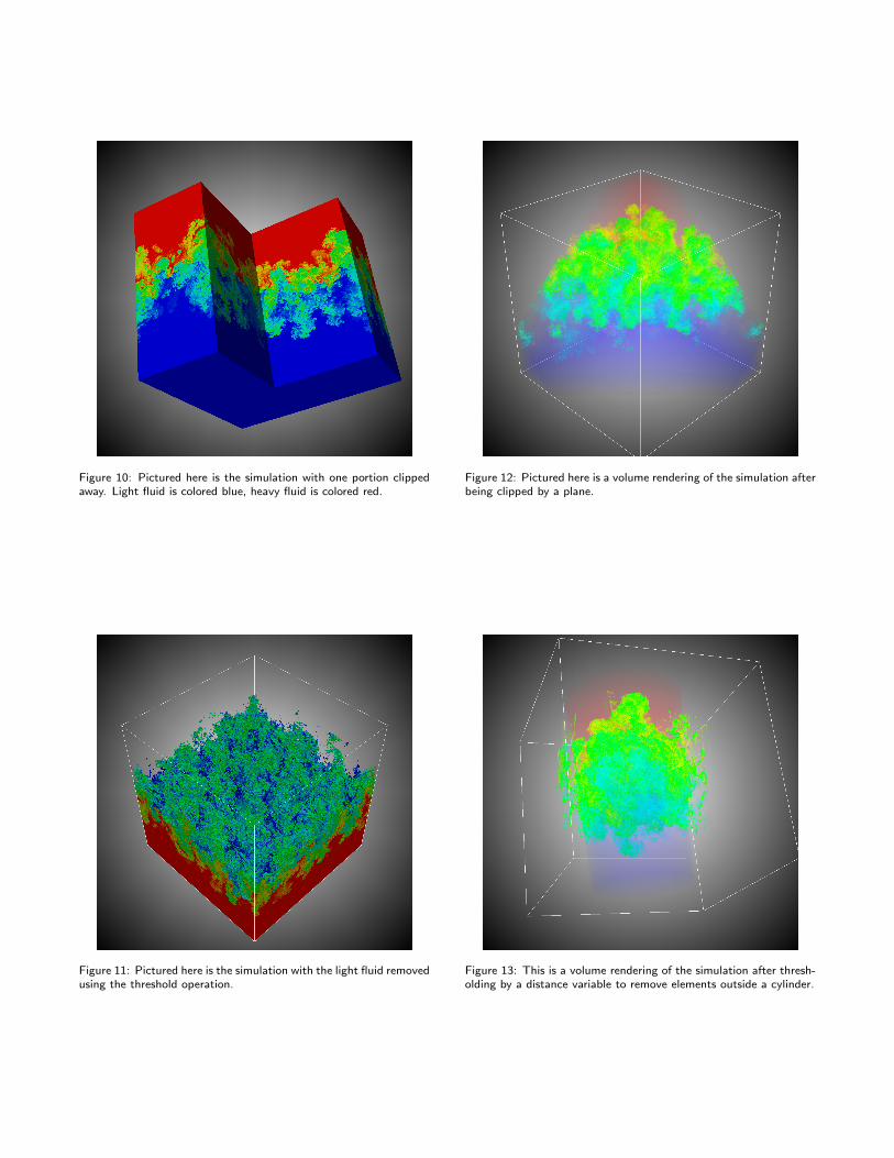
Figure 10: Pictured here is the simulation with one portion clippedaway. Light fluid is colored blue, heavy fluid is colored red.

Figure 11: Pictured here is the simulation with the light fluid removedusing the threshold operation.

Figure 12: Pictured here is a volume rendering of the simulation afterbeing clipped by a plane.

Figure 13: This is a volume rendering of the simulation after thresh-olding by a distance variable to remove elements outside a cylinder.