A Cost-Aware Path Planning Algorithm for Mobile Robots

Junghun Suh and Songhwai Oh

Abstract— In this paper, we propose a cost-aware pathplanning algorithm for mobile robots. As a robot movesfrom one location to another, the robot is penalized by thecost at its current location. The overall cost of the robotis determined by the trajectory of the robot over the costmap. The goal of the proposed cost-aware path planningalgorithm is to find the trajectory with the minimal cost. Thecost map of a field can represent environmental parameters,such as temperature, humidity, chemical concentration, wirelesssignal strength, and stealthiness. For example, if the costmap represents packet drop rates at different locations, theminimum cost path between two locations is the path with thebest possible communication, which is desirable when a robotoperates under the environment with weak wireless signals.The proposed cost-aware path planning algorithm extends therapidly-exploring random tree (RRT) algorithm by applyingthe cross entropy (CE) method for extending motion segments.We show that the proposed algorithm finds a path which isclose to the near-optimal cost path and gives an outstandingperformance compared to RRT and CE-based path planningmethods through extensive simulation.

I. INTRODUCTION

Path planning has attracted much attention in the field ofrobotics due to its importance. The goal of a path planningalgorithm is to find a continuous trajectory of a robot froman initial state to a goal state without colliding with obstacleswhile maintaining robot-specific constraints. A popular pathplanning algorithm is the rapidly-exploring random tree(RRT) [1] which is a sampling based method. It is appliedand extended by many researchers under static environments[2], [3] and dynamic environments [4], [5].

In contrast to RRT, which solves a single query problem,the probabilistic roadmap (PRM) [6] is another samplingbased path planning algorithm which is applied to solvemultiple query problems. However, since the performance isdetermined by the number of samples, importance samplingbased PRM approaches have been proposed in order toselect more samples near the region of interest (see [7]and references therein). Recently, cross entropy (CE) [8],a combination of importance sampling and optimization, hasbeen applied to path planning problems [9].

The aforementioned methods do not account for costwhich may accumulate as a robot moves. For instance, ifa robot has to travel through a dangerous environment anda map of the danger level is available, then we want tomove the robot along the path with the minimum danger.To handle such case a number of improvements have beenmade and applied to more complex cost maps in recent years[10]–[15]. In order to increase the quality of a path, the

This work has been supported in part by the Basic Science ResearchProgram through the National Research Foundation of Korea (NRF) fundedby the Ministry of Education, Science and Technology (No. 2010-0013354).

Junghun Suh and Songhwai Oh are with the School of Electrical Engi-neering and Computer Science and ASRI, Seoul National University, Seoul151-744, Korea (e-mail: {junghun.suh, songhwai.oh}@cpslab.snu.ac.kr).

nearest node of the tree to a random point is selected bycomputing the cost along the path when RRT extends a treein [10], [11], [13]. Ettlin et al. [12] applied RRT to find thepaths having low cost in rough terrain. They computed thecost of trajectories by biasing RRT towards low-cost areas.In [14], mobile robots are used to estimate environmentalparameters of the field and coordinated towards the locationwith the most information. However, they did not considerthe information gain along the trajectories of robots. In[15], Jaillet et al. presented the transition-based RRT (T-RRT) which finds low-cost paths with respect to a usergiven configuration space cost map based on a stochasticoptimization method. However, since [15] extends the treeusing a finite set of possible controls, the resulting paths canbe suboptimal.

Motivated by these developments, we propose a cost-aware navigation strategy. We assume an availability of acost map of the field of interest, which represents environ-mental parameters, such as temperature, humidity, chemicalconcentration, wireless signal strength, and stealthiness. Ourobjective is to design a path planning algorithm which guidesa robot to follow a trajectory from the initial location tothe destination with the minimal accumulated cost, alongwith the terminal cost and travel time. In this paper, the costmap of the field is represented using a Gaussian processto model complex physical phenomena. A Gaussian process(or Kriging in geostatistics) is a nonparametric regression orclassification method which has been successfully applied toestimate and predict complex physical phenomena [16].

In this paper, we present a new path planning algorithmwhich extends the RRT algorithm by applying the crossentropy method when extending motion segments as a localplanner extends the RRT tree. In contrast to the cross entropybased path planning algorithm, which can get stuck in localminima, the proposed algorithm takes advantage of RRT,which is probabilistically complete. On the other hand, theproposed method improves the quality of a trajectory byapplying cross entropy. For nonholonomic dynamics, theRRT algorithm operates by extending the tree by applyinga control from a finite set of possible controls. Hence, theresulting path from RRT is suboptimal in general. The ap-plication of cross entropy allows a search over a continuousspace of possible controls and the quality of the resultingpath is significantly better than RRT as demonstrated in thispaper.

The contribution of this paper is as follows. We firstshow that environmental parameters can be well modeledby Gaussian processes. We then propose a cost-aware pathplanning algorithm for finding the minimum cost path of arobot from one location to another based on a cost map.We demonstrate the performance of the proposed methodin simulation against RRT and cross entropy based path

planning algorithms and the near-optimal solution computedby the A∗ algorithm.

The remainder of this paper is structured as follows. InSection II, we briefly review Gaussian process regression,rapidly-exploring random trees and the cross entropy method.Section III defines the cost-aware path planning problem andexplains the proposed algorithm. The results from simulationare presented in Section IV.

II. PRELIMINARIES

A. Gaussian Process RegressionA Gaussian process (GP) is a generalization of any finite

number of random variable sets having a Gaussian distri-bution over a space of function. If z(X) is a GP, whereX ∈ D ⊆ Rn, it can be fully described by its mean functionµ(X) = E(z(X)) and covariance function K(X,X ′) =E[(z(X)−µ(X))(z(X ′)−µ(X ′))], respectively, as follows

z(X) ∼ GP(µ(X),K(X,X ′)). (1)

We can represent the data Y = [y1, y2, . . . , yn]T ∈ Rnmeasured at location X = [X1, X2, . . . , Xn] ∈ D as yi =f(Xi)+wi, where wi is a white Gaussian noise with varianceσ2w. For a new location X∗, based on the measured data Y ,

the predicted value of z(X∗) has the Gaussian distributionwith mean and variance as shown below:

z(X∗) = KT∗ (K + σ2

wI)−1Y (2)

cov(z(X∗)) = k(X∗, X∗)−KT∗ (K + σ2

wI)−1K∗ (3)

where, K = [Kij ] is the kernel matrix with (i, j) entriesKij = k(Xi, Xj), K∗ = [k(x1, x∗), . . . , k(xn, x∗)]

T , andcov(z(X∗)) is the covariance of the estimated value z(X∗)[16].

In this paper, we use the squared exponential as a kernelfunction,

k(X,X ′) = σ2f exp

(− 1

2σ2l

n∑m=1

(Xm −X ′m)

)(4)

where, σf and σl are hyperparameters of the kernel.

B. Rapidly-Exploring Random TreeThe rapidly-exploring random tree (RRT) [1] is a com-

monly used path planning algorithm, which explores a highdimensional configuration space using random sampling.Once a starting point and a goal point are defined, thealgorithm iteratively samples a random point xrand over theconfiguration space and makes an attempt to expand thesearch tree T , which is initialized with the starting point.The xrand is sampled from a uniform distribution over thespace but we can make the distribution biased towards thegoal point for faster search of a path to the goal. The tree Tis extended by connecting from xnear, which is the nearestpoint of the tree from xrand, to a new point xnew in thedirection of xrand, provided that xnear can be found. xnewis computed by applying a control input u ∈ U , where Uis a set of possible controls, to the vehicle dynamics for afixed duration 4t. Once the tree T reaches the goal point,the path can be built by searching the tree T recursively fromthe goal point to the starting point.

C. Cross Entropy Based Path PlanningCross entropy (CE) is a sampling method designed to

compute the probability of rare events [17]. It has beenalso extended to solve combinatorial optimization problems,such as the traveling salesman problem [8]. In [9], thecross entropy method is applied to path planning, wherethe optimal control law with minimum time is sought for.Algorithm 1 shows the cross entropy based path planningalgorithm which finds a trajectory for a robot from thestart position xstart to the end position xend. We samplea trajectory X from distribution p(·; v), where v is a set ofcontrols. The algorithm first generates N random trajectoriesX1, . . . , XN from p(X; vi) considering constraints such asobstacles and vehicle dynamics over the configuration space.If % > 0 is a small number, the algorithm selects %N elitetrajectory samples among all trajectory samples that haveless cost based on the cost function H , which is defined as:

H(X) =

∫ T

0

C(u(t), x(t))dt

where C = 1 + β‖x − xend‖2 with a positive constant βand T is the termination time of the trajectory [9]. Then, itupdates the parameter vi (i.e., a set of pairs of control inputand its duration) using the elite set. The algorithm iteratesuntil the sampling distribution p(X; vi) converges to a deltadistribution.

Algorithm 1 Cross Entropy Based Path PlanningInput: 1) Start position xstart and end position xend

2) Number of trajectory samples N3) Coefficients % and β

Output: the shortest time path from xstart to xend1: i = 0.2: Draw N samples X1, . . . , XN from p(X, vi), wherep(X, vi) is a uniform distribution when i = 0.

3: Select %N trajectory samples among all trajectory sam-ples that have less cost depending on cost function H .

4: Update the parameter vi using the elite set.5: i = i+ 1.6: Repeat steps 2–5 until p(X; vi) converges to a delta

function.

III. COST-AWARE PATH PLANNING

RRT and cross entropy based path planning algorithmsfind a path to the goal point considering only the length ofthe path, collision-free path, or both. However, the obtainedtrajectory may not be the optimal solution in a situationwhere environmental parameters such as temperature, hu-midity, chemical concentrations, wireless signal strength andstealthiness are represented as a cost map. Therefore, inthis section, we propose a new path planning algorithmconsidering the cost of a trajectory based on the given costmap.

A. Problem StatementLet X ⊂ Rn be the state space of a robot, where X =Xfree ∪Xobs. Xobs represents the space where obstacles areplaced or the robot may be in collision due to actuator bounds

and Xfree = X \ Xobs is a free space. Let U ∈ Rm denotethe control input space. We assume that the state of the robotx ∈ X is determined by

x = f(x, u). (5)

Let x0 ∈ X be the initial state of the robot and xgoal ⊂ Xbe the goal region. Let πu be the solution to the differentialequation (5) for given u from t = 0 to t = T . For inputu, the cost of a trajectory based on the cost map, which isdefined as C : X → R+, is defined as follows:

J(u) =

(1

T

∫ T

0

C(πu(t))dt+ CT (πu(T ))

), (6)

where T is the terminating time of the trajectory and CT :X → R+ is the terminal cost. The line integral of C alongthe path of the robot gives the quality of the robot trajectory.Now, the minimum cost path planning problem can be statedas:

minu(t):0≤t≤TJ(u)

subject to πu(t) ∈ Xfree for all t ∈ [0, T ]. (7)

The terminal cost function CT can measure, for example,how close the final state of the robot is to the goal state.The travel time of the robot can be entered into the costfunction by defining C(x) = α + Ccostmap(x), where α > 0is a coefficient used to give a different weight to the traveltime cost. There can be complications if we use (6) as a costfunction since there can be a trajectory with a lower costthan trajectories which arrive at the goal state. To avoid thisproblem, we reformulate the minimum cost path planningproblem as follows:

minu(t):0≤t≤T

(1

T

∫ T

0

C(πu(t))dt

)subject to πu(t) ∈ Xfree for all t ∈ [0, T ]

and CT (πu(T )) < τT , (8)

where τT is a small number. Hence, we find a minimum costtrajectory from a set of trajectories which ends at a locationvery near the goal state, avoiding complications which mightarise in (7).

B. Cost MapConsider the field X on which robots perform their

assigned tasks. We assume that a cost map is defined overX , representing environmental parameters. Since we cannotmeasure the environmental parameter at every location, weuse a nonparametric regression method, namely Gaussianprocess regression, to predict the environmental parameterat a site where no measurement is made.

We assume that the environmental parameter of interest,which defines the cost function C, follows a Gaussianprocess. Suppose we have made N samples from the fieldX . Let x1, x2, . . . , xN be the locations at which samplesare taken and y1, y2, . . . , yN be the measurements. Let Y =[y1, y2, . . . , yN ]T . Then, using (2), for any x∗ ∈ X , theexpected value of the cost function at x∗ is

C(x∗) = KT∗ (K + σ2

wI)−1Y.

The resulting cost map is defined over the continuous spaceX and this is different from previous approaches where costfunction is defined over a discretized space. If cost values areknown at discrete sites, the same method can be applied tosmooth the cost map. Hence, by applying Gaussian processregression, we obtain a cost map of infinite resolution. Notethat the appropriate parameters for the kernel function andthe variance of the observation model have to be learned fromthe data samples before the cost function is constructed.

C. Cost-Aware Path Planning Algorithm

We now describe a cost-aware path planning algorithmbased on RRT which uses cross entropy for extending motionsegments. The algorithm shares the overall structure as RRTas shown in Algorithm 2. However, xrand is now sampledbased on the cost map C using rejection sampling. Usingrejection sampling, we can draw samples {xrand} such thatwe obtain more samples from low cost regions than highcost regions.

The tree T initially contains only one point x0. Afterfinding the nearest point xnear of the xrand in the treeT according to the distance metric D, which is explainedin Section IV-C, we apply a modified version of the crossentropy based path planning algorithm (Algorithm 1) toextend the tree. In order to solve the modified path planningproblem (8), we define ηa and ηb. In our algorithm, we firstselect ηa trajectories with the smallest CT (πu(T )) and thenselect ηb trajectories based on the discrete-time version ofthe running cost (8) when we select an elite set for crossentropy. With this two layers of filtering, we can find asolution to (8) which always arrives at the goal region. Usingthe modified cross entropy based path planning algorithm,we find a minimum cost path from xnear to xrand. Themaximum number of iterations in the cross entropy basedpath planning algorithm is fixed to Niter in our algorithm.Only a truncated trajectory with time interval τ from thexnear is added to T . The algorithm terminates when thetree T reaches the goal region xgoal.

The proposed algorithm can reach the goal region becauseit shares the overall structure as RRT, unlike the CE basedmethod. On the other hand, while a solution from RRT isnot finely tuned to minimize the cost, the proposed algorithmenjoys fine tuning of control over a continuous control inputspace using the cross entropy based optimization.

IV. SIMULATION RESULTS

Before describing simulation results, we first describe thestate space, vehicle dynamics, and distance metric.

A. State Space

We denote the workspace (i.e., environment) as X , whereX ⊂ R2. The workspace used in simulation is [−45, 45]2.The workspace consists of two subspaces Xfree and Xobs asmentioned in III-A. Xobs contains a number of obstacles, i.e.,O1, · · · ,On ⊂ Xobs and the region where the vehicle maybe in collision with obstacles because of actuator bounds. Wecall the region the soft-obstacle zone which is similar withthe inevitable collision state in [18] and the soft-obstaclezone has radius r from each obstacle. We define Φ : X →

Algorithm 2 A cost aware navigation strategyInput: 1) Start position x0 and goal position xgoal

2) Number of trajectories Nt3) Cost map C : X → R+

4) Number of elite samples ηa, ηb5) Number of iteration Niter6) Step size τ

Output: Minimum cost path from x0 to xgoal1: Choose a sample point xrand over state space based on

rejection sampling.2: Find a point in the tree T which is nearest to xrand

according to the distance metric D.3: Apply the modified version of Algorithm 1 in order

to extend the tree T based on the cost map C. Themaximum number of iterations in Algorithm 1 is set toNiter.

4: Add the truncated trajectory for the first duration of τ .5: Repeat steps 1− 4 until tree T reaches xgoal.

R+ such that Φ(x) = 0 if d > r, Φ(x) = 1 if d = 0,and Φ(x) = 1

1+exp(−ν(d− r2 ))

if 0 < d ≤ r, where d isthe distance between x and the nearest obstacle and ν isa coefficient. In other words, Φ(x) = 0 for x ∈ Xfree,Φ(x) = 1 for x ∈ Xobs, and the soft-obstacle zone has thevalue based on Φ(x).

B. Vehicle DynamicsWe used a dynamical model of the Dubins’ car as a two-

wheeled robot in this paper. Let (px, py) be the position of arobot and θ be its heading. Suppose v(t) is the translationalvelocity and u(t) is the angular velocity, then the wholedynamics is as follows:

px(t) = v(t) cos(θ(t)), py(t) = v(t) sin(θ(t)), θ(t) = u(t),

where we fixed v as a constant and used 2m/s in simulation.A discrete-time version of the above dynamical model is usedin simulation where the sampling period ts is set to 0.1.

C. Distance MetricIn order to measure the closeness between two states of

a robot x1 = (p1x, p1y, θ

1)T and x2 = (p2x, p2y, θ

2)T weheuristically define a simple metric function D : R3×R3 →R as follows:

D(x1, x2) = ωp‖(p1x, p1y)T − (p2x, p2y)T ‖2 + ωa|θ1 − θ2|,

where ωp and ωa are positive weights for position andorientation, respectively. When ‖(p1x, p1y)T − (p2x, p

2y)T ‖2 is

smaller than threshold εb, we increased the weight ωa andfixed ωp at 1.

D. ResultsIn order to study the performance of the proposed al-

gorithm, we compared algorithm with the basic RRT (B-RRT), the cost-aware RRT (CA-RRT), the cross entropybased path planning (CEPP) algorithm, where CA-RRT is amodified RRT which finds a trajectory with the minimal costover the cost map by running the RRT algorithm multipletimes and choosing a solution with the minimum cost. We

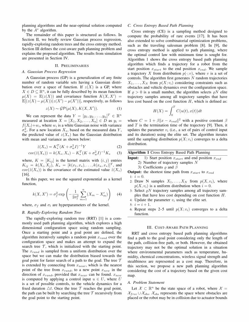
Fig. 1. Examples of scenarios used in simulation and the minimum costtrajectory found by each algorithm. The color over the field represents thecost of the field. The blue color represents low cost and the red colorrepresents high cost. The black, red, green, and blue lines represent oftrajectories found from B-RRT, CA-RRT, CEPP, and the proposed scheme,respectively.

also compared our algorithm against the near-optimal costtrajectories computed by the A∗ algorithm on a grid bydiscretizing the workspace X .

We generated five scenarios with different cost maps froma Gaussian process (1) with kernel function (4), where σ2

f =1.0 and σ2

l = 5.0. Some scenarios used in simulation areshown in Figure 1. We used the Gaussian process MATLABtoolbox [16] for modeling the cost map.

A fixed set of controls U are used for B-RRT and CA-RRT. A total of 99 controls were used from (−π2 + 0.01)to (π2 − 0.01) at an interval of 0.01. We used an adaptivenumber of Nt trajectory samples and Niter iterations in orderto reduce the computation time of extending the tree T . Weset Nt to 50 and Niter to 20, but when the xgoal point issampled as xrand, we change Nt to 100 and Niter to 50.We have found that the cross entropy based path planningtends to fail when xnear and xrand are too close. So if twopoints are too close, we use the basic RRT extension methodto extend the tree T in the proposed algorithm.

The terminal cost is defined as CT (xT ) = β‖xT −xgoal‖2where β is a positive constant and we do not include theheading of the xT for computation of CT (xT ). The numberof elite samples ηa and ηb in Section III-C are set to25 and 10, respectively, for simulation. For each scenario,ten independent trials were performed and each trial wassimulated for 600 seconds. This is the maximum deadlinefor all algorithms. We limited the number of times the treeT could be extended to 500 to reduce computation time.

We first compared our algorithm against B-RRT, CA-RRTand CEPP for each scenario without obstacles. Figure 1shows the cost map of each scenario and the minimum costtrajectory found by each algorithm. The cost map is shownas contours with different colors. The high cost region isrepresented by red and the low cost region is represented byblue. The dark circles represent the starting position and thegoal location as written in Figure 1(a) and (b). The black, red,green, and blue trajectories represent results from B-RRT,CA-RRT, CEPP, and the proposed algorithm, respectively.

Since each algorithm requires a different run time, weassigned a deadline and repeated the algorithm under eachdeadline. A solution from each method is the lowest costtrajectory from multiple runs of the algorithm until the

Deadline 200 s 300 s 400 s 500 s 600 sB-RRT 0.0779 0.0757 0.0749 0.0745 0.0739

CA-RRT 0.0404 0.0392 0.0387 0.0383 0.0378CEPP 0.0477 0.0467 0.0456 0.0451 0.0451

Proposed 0.0380 0.0369 0.0365 0.0356 0.0348

TABLE ITHE AVERAGE COSTS OF SCENARIOS WITHOUT OBSTACLES AT

DIFFERENT DEADLINES.

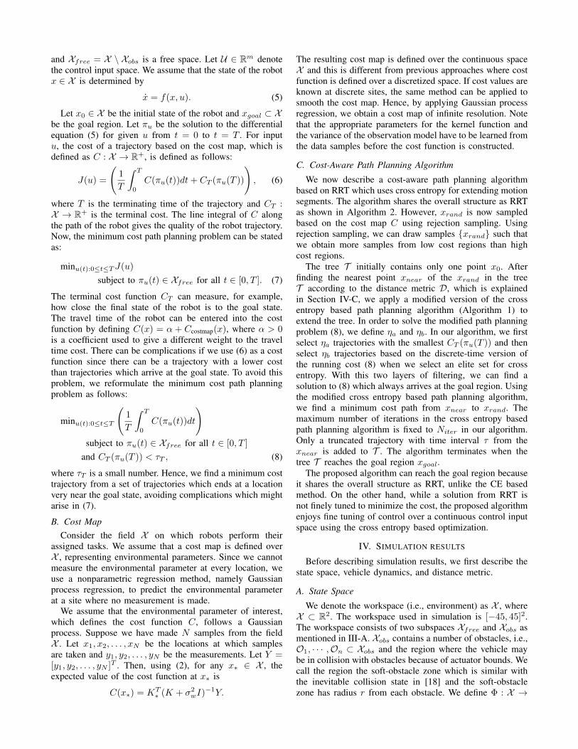
Fig. 3. Scenarios with obstacles. Only the trajectories of B-RRT (black),CA-RRT (red), the our scheme (blue) and the near-optimal trajectories foundby the A∗ algorithm (magenta) are shown since CEPP failed to arrive atthe goal region in most cases.

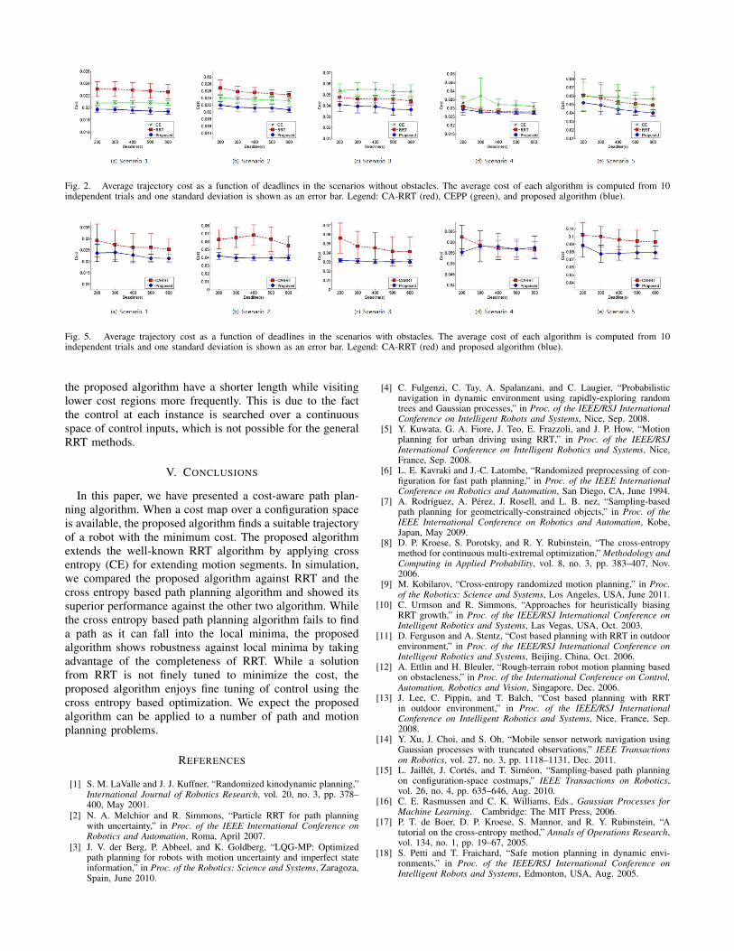
deadline. We tried 5 different deadlines from 200 secondsto 600 seconds with an interval of 100 seconds. The averagecost shown in Figure 2 is the average cost from 10 trialsfor each algorithm, along with one standard deviation errorbar. The cost of B-RRT was too high, so it is not included inFigure 2. Results from CEPP are shown in green, results fromCA-RRT are shown in red, and results from the proposedalgorithm are shown in blue. The average cost and itsvariance tend to decrease as the deadline gets longer. But themean and variance increased for CEPP between deadlines of200 and 300. This is due to the fact that the running times arenot fixed. Some runs of CEPP did not complete before 200but terminated before 300 with higher costs. The proposedalgorithm shows the lowest cost for all deadlines as shownin the figure. The average cost of each algorithm is given inTable I. The proposed algorithm shows the minimum averagecosts at all deadlines.

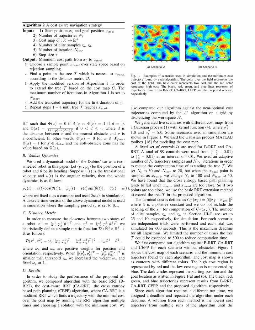
We also conducted simulations with obstacles based onthe scenarios used in the previous simulations. The minimumcost trajectory for each scenario is shown in Figure 3. Theblack thick lines represents the soft-obstacle zone includingthe obstacles. In this paper, a random sample is not chosenin this zone and any trajectory can not traverse this zone. Forscenarios with obstacles, CEPP failed in most cases as thealgorithm gets stuck at local minima. Examples of failuresfrom CEPP for the second and fourth scenarios are shownin Figure 4. The final state of the trajectories got stuck byan obstacle near the goal.

The average trajectory costs from CA-RRT and the pro-posed algorithm are shown in Figure 5. For all cases, eitherthe proposed algorithm found a lower cost trajectory ora trajectory with cost which is comparable to that of atrajectory found by CA-RRT. The average cost of eachalgorithm is given in Table II. When compared to the near-

Fig. 4. Examples of failure from CEPP. The green trajectories did notreach the goal and got stuck by an obstacle.

Deadline 200 s 300 s 400 s 500 s 600 sB-RRT 0.0951 0.0861 0.0853 0.0842 0.0826

CA-RRT 0.0600 0.0575 0.0553 0.0531 0.0509Proposed 0.0471 0.0458 0.0448 0.0441 0.0440

TABLE IITHE AVERAGE COSTS OF SCENARIOS WITH OBSTACLES AT DIFFERENT

DEADLINES.

Algorithm B-RRT CA-RRT Proposed A∗

Cost 0.0580 0.0443 0.0391 0.0354Trajectory Length 661 753 703 622

TABLE IIITHE AVERAGE COSTS AND TRAJECTORY LENGTHS FOR ALL SCENARIOS

WITH OBSTACLES

Algorithm Scenario 1 2 3 4 5

CA-RRT No. Runs 92 63 79 182 76No. Successes 57 26 47 154 37

CEPP No. Runs 40 68 70 90 90No. Successes 0 1 1 1 1

Proposed No. Runs 32 22 28 23 19No. Successes 31 18 26 23 19

TABLE IVTHE NUMBER OF RUNS AND SUCCESSFUL RUNS FROM EACH

ALGORITHM BEFORE THE MAXIMUM DEADLINE (600S) FOR SCENARIOS

WITH OBSTACLES.

optimal cost paths by the A∗ algorithm, the cost of oursis only 10% higher than the cost of the near-optimal costpaths as shown in Table III. Also, the trajectories from theproposed algorithm are very similar to the near-optimal pathsfound by the A∗ algorithm (see Figure 3 for an example).Notice that the proposed algorithm achieves the preformancewhich is comparable to the near-optimal solution found bythe A∗ algorithm at a fraction of computation time comparedto the A∗ algorithm, which requires over 12 hours to computea near-optimal cost path. Furthermore, the success rate of theproposed method is much higher than CA-RRT, showing therobustness of the proposed method against local minima. Thenumber of runs and successful runs, i.e., when a trajectoryarrives at the goal region, from each algorithm are shown inTable IV.

As can be seen from Figure 3, the trajectories found by

Fig. 2. Average trajectory cost as a function of deadlines in the scenarios without obstacles. The average cost of each algorithm is computed from 10independent trials and one standard deviation is shown as an error bar. Legend: CA-RRT (red), CEPP (green), and proposed algorithm (blue).

Fig. 5. Average trajectory cost as a function of deadlines in the scenarios with obstacles. The average cost of each algorithm is computed from 10independent trials and one standard deviation is shown as an error bar. Legend: CA-RRT (red) and proposed algorithm (blue).

the proposed algorithm have a shorter length while visitinglower cost regions more frequently. This is due to the factthe control at each instance is searched over a continuousspace of control inputs, which is not possible for the generalRRT methods.

V. CONCLUSIONS

In this paper, we have presented a cost-aware path plan-ning algorithm. When a cost map over a configuration spaceis available, the proposed algorithm finds a suitable trajectoryof a robot with the minimum cost. The proposed algorithmextends the well-known RRT algorithm by applying crossentropy (CE) for extending motion segments. In simulation,we compared the proposed algorithm against RRT and thecross entropy based path planning algorithm and showed itssuperior performance against the other two algorithm. Whilethe cross entropy based path planning algorithm fails to finda path as it can fall into the local minima, the proposedalgorithm shows robustness against local minima by takingadvantage of the completeness of RRT. While a solutionfrom RRT is not finely tuned to minimize the cost, theproposed algorithm enjoys fine tuning of control using thecross entropy based optimization. We expect the proposedalgorithm can be applied to a number of path and motionplanning problems.

REFERENCES

[1] S. M. LaValle and J. J. Kuffner, “Randomized kinodynamic planning,”International Journal of Robotics Research, vol. 20, no. 3, pp. 378–400, May 2001.

[2] N. A. Melchior and R. Simmons, “Particle RRT for path planningwith uncertainty,” in Proc. of the IEEE International Conference onRobotics and Automation, Roma, April 2007.

[3] J. V. der Berg, P. Abbeel, and K. Goldberg, “LQG-MP: Optimizedpath planning for robots with motion uncertainty and imperfect stateinformation,” in Proc. of the Robotics: Science and Systems, Zaragoza,Spain, June 2010.

[4] C. Fulgenzi, C. Tay, A. Spalanzani, and C. Laugier, “Probabilisticnavigation in dynamic environment using rapidly-exploring randomtrees and Gaussian processes,” in Proc. of the IEEE/RSJ InternationalConference on Intelligent Robots and Systems, Nice, Sep. 2008.

[5] Y. Kuwata, G. A. Fiore, J. Teo, E. Frazzoli, and J. P. How, “Motionplanning for urban driving using RRT,” in Proc. of the IEEE/RSJInternational Conference on Intelligent Robotics and Systems, Nice,France, Sep. 2008.

[6] L. E. Kavraki and J.-C. Latombe, “Randomized preprocessing of con-figuration for fast path planning,” in Proc. of the IEEE InternationalConference on Robotics and Automation, San Diego, CA, June 1994.

[7] A. Rodrıguez, A. Perez, J. Rosell, and L. B. nez, “Sampling-basedpath planning for geometrically-constrained objects,” in Proc. of theIEEE International Conference on Robotics and Automation, Kobe,Japan, May 2009.

[8] D. P. Kroese, S. Porotsky, and R. Y. Rubinstein, “The cross-entropymethod for continuous multi-extremal optimization,” Methodology andComputing in Applied Probability, vol. 8, no. 3, pp. 383–407, Nov.2006.

[9] M. Kobilarov, “Cross-entropy randomized motion planning,” in Proc.of the Robotics: Science and Systems, Los Angeles, USA, June 2011.

[10] C. Urmson and R. Simmons, “Approaches for heuristically biasingRRT growth,” in Proc. of the IEEE/RSJ International Conference onIntelligent Robotics and Systems, Las Vegas, USA, Oct. 2003.

[11] D. Ferguson and A. Stentz, “Cost based planning with RRT in outdoorenvironment,” in Proc. of the IEEE/RSJ International Conference onIntelligent Robotics and Systems, Beijing, China, Oct. 2006.

[12] A. Ettlin and H. Bleuler, “Rough-terrain robot motion planning basedon obstacleness,” in Proc. of the International Conference on Control,Automation, Robotics and Vision, Singapore, Dec. 2006.

[13] J. Lee, C. Pippin, and T. Balch, “Cost based planning with RRTin outdoor environment,” in Proc. of the IEEE/RSJ InternationalConference on Intelligent Robotics and Systems, Nice, France, Sep.2008.

[14] Y. Xu, J. Choi, and S. Oh, “Mobile sensor network navigation usingGaussian processes with truncated observations,” IEEE Transactionson Robotics, vol. 27, no. 3, pp. 1118–1131, Dec. 2011.

[15] L. Jaillet, J. Cortes, and T. Simeon, “Sampling-based path planningon configuration-space costmaps,” IEEE Transactions on Robotics,vol. 26, no. 4, pp. 635–646, Aug. 2010.

[16] C. E. Rasmussen and C. K. Williams, Eds., Gaussian Processes forMachine Learning. Cambridge: The MIT Press, 2006.

[17] P. T. de Boer, D. P. Kroese, S. Mannor, and R. Y. Rubinstein, “Atutorial on the cross-entropy method,” Annals of Operations Research,vol. 134, no. 1, pp. 19–67, 2005.

[18] S. Petti and T. Fraichard, “Safe motion planning in dynamic envi-ronments,” in Proc. of the IEEE/RSJ International Conference onIntelligent Robots and Systems, Edmonton, USA, Aug. 2005.