A Coupled Ice-Ocean Model in the Pan-Arctic and NorthAtlantic Ocean: Simulation of Seasonal Cycles
JIA WANG1*, QINZHENG LIU2, MEIBING JIN1, MOTOYOSHI IKEDA3 and FRANCOIS J. SAUCIER4
1International Arctic Research Center, University of Alaska Fairbanks, Fairbanks, AK 99775, U.S.A.2Center for Marine Environmental Forecasts, State Oceanic Administration, Beijing, China3Graduate School of Environmental Earth Science, Hokkaido University, Sapporo 060-0810, Japan4Maurice Lamontagne Institute, Department of Fisheries and Oceans, Mont-Joli, Quebec G5H 3Z4, Canada
(Received 29 September 2003; in revised form 22 June 2004; accepted 22 June 2004)
A coupled ice-ocean model is configured for the pan-Arctic and northern North At-lantic Ocean with a 27.5 km resolution. The model is driven by the daily atmosphericclimatology averaged from the 40-year NCEP reanalysis (1958–1997). The ocean modelis the Princeton Ocean Model (POM), while the sea ice model is based on a full ther-modynamical and dynamical model with plastic-viscous rheology. A sea ice modelwith multiple categories of thickness is utilized. A systematic model-data comparisonwas conducted. This model reasonably reproduces seasonal cycles of both the sea iceand the ocean. Climatological sea ice areas derived from historical data are used tovalidate the ice model performance. The simulated sea ice cover reaches a maximumof 14 ××××× 106 km2 in winter and a minimum of 6.7 ××××× 106 km2 in summer. This is close tothe 95-year climatology with a maximum of 13.3 ××××× 106 km2 in winter and a minimumof 7 ××××× 106 km2 in summer. The simulated general circulation in the Arctic Ocean, theGIN (Greenland, Iceland, and Norwegian) seas, and northern North Atlantic Oceanare qualitatively consistent with historical mapping. It is found that the low wintersalinity or freshwater in the Canada Basin tends to converge due to the strong anticy-clonic atmospheric circulation that drives the anticyclonic ocean surface current, whilelow summer salinity or freshwater tends to spread inside the Arctic and exports outof the Arctic due to the relaxing wind field. It is also found that the warm, salineAtlantic Water has little seasonal variation, based on both simulation and observa-tions. Seasonal cycles of temperature and salinity at several representative locationsreveals regional features that characterize different water mass properties.
ter budget, deep water convection, as well as heat andsalt flux (Ikeda, 1990; Ikeda et al., 2001). Global climatemodels (Holland et al., 2001; Saenko et al., 2002), or atleast the pan-Arctic coupled ice-ocean models, (Chengand Preller, 1992; Oberhuber, 1993; Weatherly and Walsh,1996; Wang et al., 2002; Köberle and Gerdes, 2003) arenecessary to reveal the seasonal, interannual, and decadalvariability of the coupling system.
There have been some investigations of Arctic ice-ocean circulation using limited domain models with theNorth Atlantic Ocean excluded (Semtner, 1976; Hiblerand Bryan, 1987; Fleming and Semtner, 1991; Hakkinenet al., 1992; Zhang et al., 2000; Polyakov, 2001; Zhangand Zhang, 2001). The limited region models with thesouthern boundary at the Denmark Strait decouple theArctic ice-ocean system with the North Atlantic circula-tion system, with the natural interactions between the
1. IntroductionThe pan-Arctic and North Atlantic Ocean is a natu-
ral atmosphere-ice-ocean coupling system (Mysak et al.,1990; Ikeda, 1990; Wang et al., 2004). The North Atlan-tic Oscillation (NAO, van Loon and Rogers, 1978; Hurreland van Loon, 1997) is a key atmospheric componentdriving ocean circulation and exchanging momentum andmass with sea ice and ocean. Thus, the Arctic Ocean cir-culation (Fig. 1(a); Coachman and Aagaard, 1974;Aagaard, 1981, 1989; Jones et al., 1995) and sea ice flow(Pfirman et al., 1997; Rigor et al., 2002) have a strongcoupling to the North Atlantic Ocean circulation (Fig.1(b)) in terms of water exchange and transport, freshwa-
214 J. Wang et al.
Arctic-GIN (Greenland, Iceland, and Norwegian, or Nor-dic) Seas and the North Atlantic Ocean excluded (Mysaket al., 1990; Ikeda, 1990; Ikeda et al., 2001; Wang et al.,2005), although the interannual and decadal variabilityof the ice-ocean system can be driven by the atmosphericforcing within the Arctic Ocean.
Coupled ice-ocean models can be categorized intothree groups in terms of vertical coordinates: z-coordi-nate models (Cheng and Preller, 1992; Weatherly andWalsh, 1996; Karcher et al., 1999; Zhang et al., 2000;Maslowski et al . , 2001; Zhang and Zhang, 2001;Polyakov, 2001), sigma-coordinate models (Hakkinen,2000; Wang et al., 2002), and isopynal-coordinate mod-els (Oberhuber, 1993). Sea ice models are based on twotypes of rheology: viscous-plastic (Hibler, 1979), and elas-
tic-viscous-plastic (Hunke and Dukowicz, 1997). An iso-tropic sea ice property is assumed because large-scale seaice dynamics is considered. An Arctic Ocean ModelsIntercomparison Project (AOMIP) has been conducted tocompare a variety of parameters and physical processesunder the same forcing, but with different, stand-aloneconfigurations, resolutions, coupling techniques and co-ordinates (Proshutinsky et al., 2001). The purpose is toreveal physical processes in response to the same atmos-pheric forcing without examining the details of the otherfactors mentioned above.
Most previous studies conducted model-data com-parison mainly using surface information such as sea iceconcentration (area), thickness, sea ice drift, and surfaceocean circulation. Few of them compared their results withobservations in a deep layer, such as the Atlantic Layerbecause the Atlantic Layer is very sensitive to many fac-tors. Very often, this layer cannot be reproduced becauseof large diffusivity imbedded in a model. Thus, this studywill provide a systematic model-data comparison includ-ing the deep Atlantic Layer and other direct variables, aswell as other indirect parameters such as freshwater stor-age and heat content (Zhang and Zhang, 2001).
The ocean model used in this study is the POM(Princeton Ocean Model, Blumberg and Mellor, 1987).Although a sigma-coordinate model may have difficultyin dealing with steep topography (Haney, 1991), it hasperformed well in the coastal ocean with less steep orheavily smoothed topography (Mellor et al., 1994; Wang,2001). Some models use a simple one-layer sea ice model(Hibler, 1979) plus one layer of snow. In this study weuse a sea ice model with multiple categories of sea icethickness (Throndike et al., 1975; Hibler, 1980; Yao etal., 2000; Wang et al., 2002). The purpose is to furtherresolve thin ice to first-year ice, and multi-year ice(Haapala, 2000) in the near future. The motivation of thismodeling exercise is to investigate the seasonal variationsof the sea ice-ocean circulation system in the study re-gion using the 3-D coupled ice-ocean model. This pro-vides a foundation for further studies of interannual anddecadal variability in the region (Wang et al., 2005).
The following section describes the models. Section3 presents the seasonal cycles of sea ice and ocean circu-lation. In Section 4, we conduct diagnostic analyses ofseasonal cycles of temperature, salinity sections, and dif-ferent locations. A summary is given in Section 5.
2. Model DescriptionThis coupled ice-ocean model was described in great
detail in the model development and application to thepan-Arctic region (Wang et al., 2002). In the following,we only describe the parts necessary for the complete-ness of this paper.
a)
b)
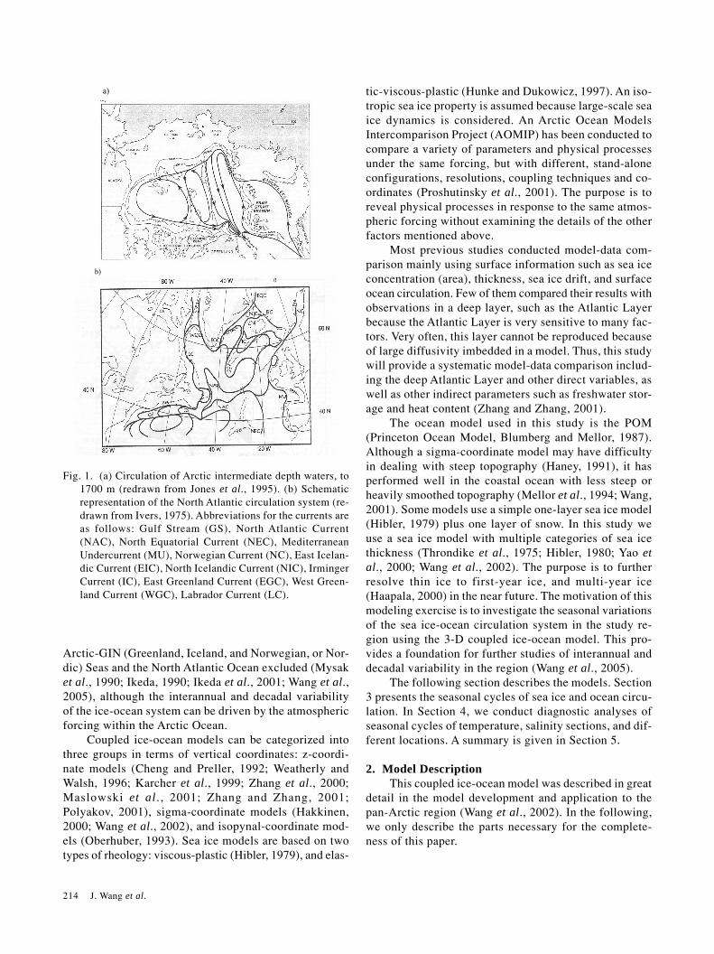
Fig. 1. (a) Circulation of Arctic intermediate depth waters, to1700 m (redrawn from Jones et al., 1995). (b) Schematicrepresentation of the North Atlantic circulation system (re-drawn from Ivers, 1975). Abbreviations for the currents areas follows: Gulf Stream (GS), North Atlantic Current(NAC), North Equatorial Current (NEC), MediterraneanUndercurrent (MU), Norwegian Current (NC), East Icelan-dic Current (EIC), North Icelandic Current (NIC), IrmingerCurrent (IC), East Greenland Current (EGC), West Green-land Current (WGC), Labrador Current (LC).
A Coupled Ice-Ocean Model in the Pan-Arctic and North Atlantic Ocean: Simulation of Seasonal Cycles 215
2.1 Sea-ice modelThe sea ice component of the coupled model is a ther-
modynamic model based on multiple categories of icethickness distribution function (Throndike et al., 1975;Hibler, 1980) and a dynamic model based on a viscous-plastic sea ice rheology (Hibler, 1979).
The evolution of the thickness distribution functionsatisfies a continuity equation
∂∂
+ ∇ ⋅ ( ) = −∂( )
∂+ ( )g
tVg
gh
h
rψ 1
where rV is velocity vector (u, v), g is the sea ice thick-
ness distribution function, and g(h)dh is defined as thefraction of area covered by the ice with thickness betweenh and h + dh. The averaged thickness h and concentra-tion A of sea ice in a grid is expressed from g(h) as
A g h dhh
= ( ) ( )+∫0
2
and
h g h hdhh
= ( ) ( )∫03
ψ is the mechanical redistribution function, which repre-sents the creation of open water and ridging during icedeformation. The redistribution process conserves icevolume. The redistribution function is parameterized asdescribed by Yao et al. (2000). f(h) is the thermodynamicvertical growth rate of ice.
The vertical growth rate f(h) of ice thickness is de-termined by the ice thermodynamics. The model thermo-dynamic interactions between ice, ocean and atmosphereare shown in Fig. 2. The heat budget on the upper icesurface is
QAI = QSi + QEi + QL + (1 – α i)I0 – εiσT04 (4)
where α i is the albedo of sea ice (0.75 during the freezingperiod from October to March, 0.65 during the melting
period from April to September). When snow exists, icealbedo is replaced by the snow albedo αs (0.9); εi is theemissivity of ice. I0 is the short wave solar radiation reach-ing the ice surface; QSi, QEi, and QL are the sensible heatflux, the latent heat flux, and the effective longwave ra-diation flux from ice surface, respectively. QSi, QEi andQL are parameterized by the following formulae,
where qa and Ta are the specific humidity and air tem-perature of air; q0 is the saturated specific humidity onice; T0 is the surface ice temperature. Cp is the specificheat of air at constant pressure. Le is the latent heat sub-limation on the ice surface. Cs and Ce are the sensibleheat and latent heat bulk transfer coefficients, respectively.εa is the emissivity of air. σ is Stefan-Boltzman constant.kc is the cloud factor and CL is the cloud fraction. Ta isthe air temperature, a and b are empirical constants (a =0.254, b = 4.95 × 10⁻⁵). The surface ice temperature T0 isdetermined from the surface heat balance equation,
QAI – Qc = 0 (8)
where Qc is the internal conductive heat flux through ice.A linear ice temperature profile and a constant thermalconductive coefficient ki are used in this study. Thus, forthe ice category with thickness h,
Qc = –ki(T0 – Tf)/h (9)
where Tf is the freezing temperature of seawater on bot-tom ice surface, which is a function of the salinity ofseawater (=–0.0544S0 + 237.15K, where S0 is the salinityof upmost ocean grid, in part per thousand, ppt). For thesnow-covered ice, the conductive coefficient will be re-placed by (kiks)/(hks + hski), where hs is the snow depth.
If the calculated T0 is found to be over 0°C, it isforced to be 0°C. The extra heat of Eq. (8) is used to meltthe ice at the upper surface, and the melted water willdrain to the ocean immediately. The volume flux of melt-ing water WAI is
WAI = [QAI – Qc]/L. (10)
The growth rate at the bottom of the sea ice is
WIW = [Qc – FT]/L (11)
I0 αiI0 QSi QEi QL εiσT0
4
I0 αwI0 QSw QEw QLw εwσTw4
snow
Sea Ice Fc Water surface
Fw Fw
Fig. 2. Interactions among the air, ice, and ocean system interms of thermodynamics.
216 J. Wang et al.
where L is the volume latent heat of fusion and FT is theoceanic heat flux out of the ocean surface (assumed to beuniform over a model grid cell). Thus, the growth ratef(h) for sea ice with thickness h is the sum of (10) and(11), i.e.
f(h) = (QAI – FT]/L. (12)
For the open water in the ice zone, the growth rateof sea ice is
WAW = (QAW – FT)/L (13)
where QAW is the heat budget between the atmosphere-ocean interface, excluding the solar radiation that is ab-sorbed in the water column. QAW is calculated using asimilar parameterization to (4) but without the solar ra-diation terms, i.e.
QAW = QSw + QEw + QLw – εwσTw4 (14)
where εw is the emissivity of water. Tw is the sea surfacetemperature (SST). QSw , QEw , and QL are the sensibleheat flux, the latent heat flux and the effective longwaveradiation flux from water surface, which are parameterizedsimilar to (5)–(7). When the WAW is negative, the “melt-ing” of ice to water is implied. In this case, the equiva-lent heat is redistributed to melt the remaining ice. Thetotal ice growth rate is integral over various ice thick-nesses with weight g(h).
The ice velocity rV is determined from the momen-
tum equation
m
dV
dtmfk V mg H F
vv v r v v
+ × = − ∇ + − + ( )τ τa w 15
where f is the Coriolis force and m is the ice mass in agrid. ∇ H is the gradient of sea surface elevation,
vF is the
internal stresses (see Hibler, 1979; Wang et al., 1994a),and
rτ a and
vτ w are the air and water stresses, respectively.They are determined by the bulk formulae
r r rτ ρa a a a a= C V V 16( )
v r r r rτ ρw w w w i w i= − −( ) ( )C V V V V 17
where rVa is wind velocity vector.
rVw is the current ve-
locity vector of the upmost ocean layer. Ca (=1.2 × 10⁻³)and Cw (=5.5 × 10⁻³) are the bulk coefficients of windstress and water stress, respectively. ρa is the air density,and ρw the seawater density.
vF is the two-dimensional
internal ice stress tensor, which is derived from the vis-
cous plastic rheology with elliptical yield curve rate e =2 of Hibler (1979) and involves a compressive ice strength
P P h C A= × − −( )[ ] ( )∗ exp 1 18
where P* and C are empirical constants (here 2.5 × 10⁴
Nm–2 and 20, respectively). e is the ratio of principal axesof the ellipse, P* is the ice strength, and C is the icestrength decay constant. This formulation requires thatthe ice strength strongly depends on the amount of thinice, characterized by (1 – A), which is also allows the iceto strengthen as it becomes thicker, as measured by thick-ness h .
The redistribution function is parameterized as de-scribed by Thorndike et al. (1975) and Yao et al. (2000).Unlike the treatment by Hibler (1980), they used a giventhickness to ridged ice of a single thickness (the multi-plication factor is chosen as 15). Table 1 lists the param-eters, their values and units that are used in this model.
2.2 Ocean modelThe Princeton Ocean Model (Blumberg and Mellor,
1987; Wang, 2001) is used as the ocean component of thecoupled mode in this study. The model has a free surface,uses sigma coordinates in the vertical, and employs amode-split technique. The model embeds a second-orderturbulence closure sub-model. Smagorinsky diffusivityalong sigma surfaces is employed in the horizontal diffu-sion.
The governing equations of temperature and salt are
∂∂
+ ∇ ⋅ ( ) + ∂∂
= ∂∂
∂∂
+ − −( ) ∂∂( )
T
tV T
TK
TF
Ivw H T w
ωσ σ σ
σσ
1
19
0
∂∂
+ ∇ ⋅ ( ) + ∂∂
= ∂∂
∂∂
+ ( )S
tV S
SK
SF
vw H S
ωσ σ σ
20
and the surface heat forcing is
QAW = QSw + QEw + QLw – εwσTw4 (21)
in the ice-free grid cell, and
A × FT + (1 – A)QAW (22)
in the ice-covered grid cell.
2.3 Ice-ocean couplingHeat and salt fluxes at the ice-ocean interface are
governed by the boundary processes as discussed byMellor and Kantha (1989) and Kantha and Mellor (1989).
A Coupled Ice-Ocean Model in the Pan-Arctic and North Atlantic Ocean: Simulation of Seasonal Cycles 217
In grid cells in which ice is present, the heat flux out ofthe ocean is
FT = –ρwCpCTz(Tf – T) (23)
where Cp is the specific heat of seawater and T is the oceantemperature at the uppermost model grid (in our modelthe midpoint of the uppermost ocean layer). The heattransfer coefficient CTz is given by
Cu
P z z k BTzrt T
=−( ) +
( )∗
ln / /0
24
BT = b(z0u∗ /v)1/2Pr2/3
where u∗ is the friction velocity, Prt is a turbulent Prantl
number, z is the vertical coordinate corresponding to thetemperature T, z0 is the roughness length, and k is the vonKarman constant. The molecular sublayer correction isrepresented by BT where Pr is a molecular Prantl number,v is the kinematic viscosity, and b is an empirical con-stant (=3). The salt flux out of the ocean is
where SI is the salinity of ice (=5‰), S is the salinity atthe uppermost model grid point, and (P – E) is the vol-ume flux of precipitation minus evaporation.
Analogous to the heat flux (23), the salt flux is de-fined as
FS = –CSz(S0 – S) (26)
Table 1. Constants used in CIOM.
Symbols Description Values Units
a empirical constant 0.254b empirical constant 4.95 × 10⁻⁵
CS sensible heat bulk transfer coef. 2.32× 10⁻³ when Ts < Ta
1.75× 10⁻³ when Ts >= Ta
CP specific heat of air 1410 J kg–1K–1
CP,W specific heat of sea water 3903 J kg–1K–1
e yield curve eccentricity 2ei emission of sea ice 0.65–0.75L volume latent heat of fusionLe latent heat sublimation on ice surface 3.32 × 10⁻³
k von Karman constant 0.4k C cloud factor 0.62k i thermal conductive coef. 2.04P* ice strength 2.5 × 10⁴ Nm–2
Pr molecular Prantl number 12.9ρa air density 1.3 kg m–3
ρi sea ice density 910 kg m–3
ρw seawater density 1025 kg m–3
S I sea ice salinity 5‰Sc Schmidt number 2432σ Stefan-Boltzman constant 5.67 × 10⁻⁸
∆x = ∆y model horizontal grid size 27500 m
∆T time step for eternal mode 45 seconds
∆t time step for internal mode and ice 1800 seconds
218 J. Wang et al.
where S0 is the salinity at the ice-ocean interface. Thesalt transfer coefficient CSz is
Cu
P z z k BSzrt S
=−( ) +
( )∗
ln / /0
27
BS = b(z0u∗ /v)1/2Sc2/3
where Sc is a Schmidt number. Since Sc = 2432 and Pr =12.9, CTz > CSz, this can lead to the production of frazilice in the water column as discussed by Mellor and Kantha(1989). Frazil ice is immediately added to the floatingice.
The ice-water stress is
τ ρw w i w/ln /
= ( ) −( )∗ku
z zV V
0
r r
where rVw is the ocean velocity vector at the uppermost
model grid.
2.4 Model configuration and atmospheric forcingThe model grid size is 27.5 km with 16 sigma lay-
ers. The domain includes the central Arctic Ocean (Canadaand Eurasian Basins), GIN Seas, Canadian Archipelago,
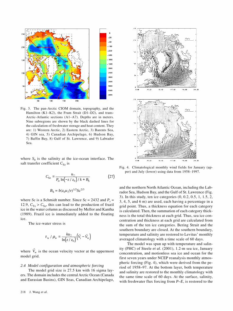
and the northern North Atlantic Ocean, including the Lab-rador Sea, Hudson Bay, and the Gulf of St. Lawrence (Fig.3). In this study, ten ice categories (0, 0.2, 0.5, 1, 1.5, 2,3, 4, 5, and 6 m) are used, each having a percentage in agrid point. Thus, a thickness equation for each categoryis calculated. Then, the summation of each category thick-ness is the total thickness at each grid. Thus, sea ice con-centration and thickness at each grid are calculated fromthe sum of the ten ice categories. Bering Strait and thesouthern boundary are closed. At the southern boundary,temperature and salinity are restored to Levitus’ monthlyaveraged climatology with a time scale of 60 days.
The model was spun up with temperature and salin-ity (PHC) of Steele et al. (2001), 1.2-m sea ice, Januaryconcentration, and motionless sea ice and ocean for thefirst seven years under NCEP reanalysis monthly atmos-pheric forcing (Fig. 4), which were derived from the pe-riod of 1958–97. At the bottom layer, both temperatureand salinity are restored to the monthly climatology withthe same time scale of 60 days. At the surface, salinity,with freshwater flux forcing from P–E, is restored to the
1 23
45
67
8
9
Fig. 3. The pan-Arctic CIOM domain, topography, and theHamilton (K1–K2), the Fram Strait (D1–D2), and trans-Arctic-Atlantic sections (A1–A7). Depths are in meters.Nine subregions are shown by the black dashed lines forthe calculation of freshwater storage and heat content. Theyare: 1) Western Arctic, 2) Eastern Arctic, 3) Barents Sea,4) GIN sea, 5) Canadian Archipelago, 6) Hudson Bay,7) Baffin Bay, 8) Gulf of St. Lawrence, and 9) LabradorSea.
Fig. 4. Climatological monthly wind fields for January (up-per) and July (lower) using data from 1958–1997.
A Coupled Ice-Ocean Model in the Pan-Arctic and North Atlantic Ocean: Simulation of Seasonal Cycles 219
observed monthly salinity fields at a time scale of 30 daysfor prescribing freshwater runoff into the Arctic Basinusing the flux correction method of Wang et al. (2001).After a seven-year spinup, a dynamical and thermody-namical seasonal cycle is established (Fig. 5). Then, were-ran the model for another six years using the seventhyear output as the restart or initial conditions. During thesix-year run, all the monthly atmospheric forcings remainthe same, except when the daily wind fields are used.Then, the last three-year averaged variables are used forexamining the seasonal cycle in this study.
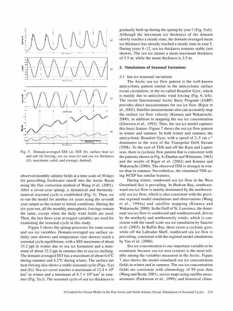
Figure 5 shows the spinup processes for some oceanand sea ice variables. Domain-averaged sea surface sa-linity (not shown) and temperature (not shown) reach aseasonal cycle equilibrium, with a SSS maximum of about33.2 ppt in winter due to sea ice formation and a mini-mum of about 32.2 ppt in summer due to sea ice melting.The domain-averaged SST has a maximum of about 6.6°Cduring summer and 4.2°C during winter. The surface netheat forcing also shows a stable seasonal cycle (Figs. 5(a)and (b)). Sea ice cover reaches a maximum of 12.4 × 10⁶
km2 in winter and a minimum of 8.7 × 10⁶ km2 in sum-mer (Fig. 5(c)). The seasonal cycle of sea ice thickness is
gradually built up during the spinup by year 7 (Fig. 5(d)).Although the maximum ice thickness of the domainslowly reaches a steady state, the domain-averaged meanice thickness has already reached a steady state in year 5.During years 8–12, sea ice thickness remains stable (notshown). The sea ice attains a mean maximum thicknessof 5.5 m, while the mean thickness is 2.5 m.
3. Simulations of Seasonal Variations
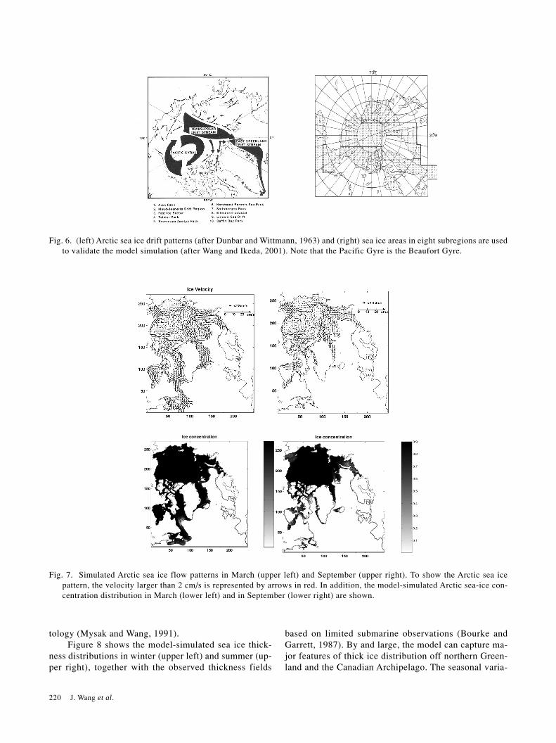
3.1 Sea ice seasonal variationsThe Arctic sea ice flow pattern is the well-known
anticyclonic pattern similar to the anticyclonic surfaceocean circulation, or the so-called Beaufort Gyre, whichis mainly due to anticylonic wind forcing (Fig. 6, left).The recent International Arctic Buoy Program (IABP)provides direct measurements for sea ice flow (Rigor etal., 2002). Satellite measurements also can accurately mapthe surface ice flow velocity (Kimura and Wakatsuchi,2000), in addition to mapping the sea ice concentration(Gloersen et al., 1992). Thus, the sea ice model capturesthis basic feature. Figure 7 shows the sea ice flow patternin winter and summer. In both winter and summer, theanticyclonic Beaufort Gyre, with a speed of 2–5 cm s–1
dominates to the west of the Transpolar Drift Stream(TDS). To the east of TDS and off the Kara and Laptevseas, there is cyclonic flow pattern that is consistent withthe patterns shown in Fig. 6 (Dunbar and Wittmann, 1963)and the results of Rigor et al. (2002) and Kimura andWakatsuchi (2000). The observed TDS is stronger in win-ter than in summer. Nevertheless, the simulated TDS us-ing NCEP has similar features.
During winter, southward sea ice flow in the WestGreenland Sea is prevailing. In Hudson Bay, southeast-ward sea ice flow is mainly dominated by the northwest-erly sea ice flow, which is also consistent with the previ-ous regional model simulations and observations (Wanget al., 1994a) and satellite mapping (Kimura andWakatsuchi, 2000). In the Gulf of St. Lawrence, the domi-nant sea ice flow is southward and southeastward, drivenby the northerly and northeasterly winds, which is con-sistent with the small-scale sea ice simulation by Saucieret al. (2003). In Baffin Bay, there exists a cyclonic gyre,while off the Labrador Shelf, southward sea ice flow isprevailing, consistent with the regional model simulationsby Yao et al. (2000).
Sea ice concentration is one important variable to beexamined, because sea ice area (extent) is the most reli-able among the variables measured in the Arctic. Figure7 also shows the model-simulated sea ice concentrationfields in winter and in summer. The sea ice concentrationfields are consistent with climatology of 95-year data(Wang and Ikeda, 2001), sea ice maps using satellite meas-urements (Parkinson et al., 1999), and historical clima-
a)
b)
c)
d)
Fig. 5. Domain-averaged SSS (a), SST (b), surface heat (c)and salt (d) forcing, sea ice area (e) and sea ice thickness((f), maximum: solid, and average: dashed).
220 J. Wang et al.
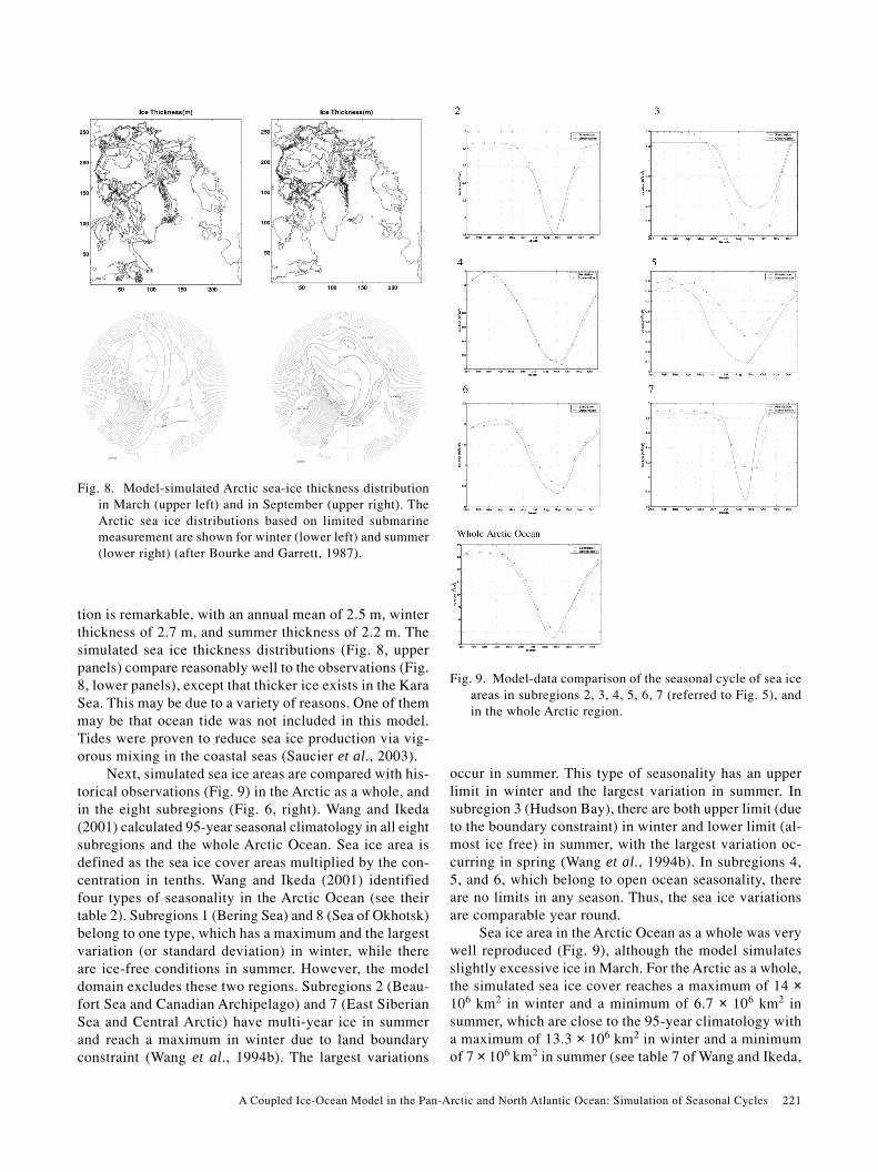
tology (Mysak and Wang, 1991).Figure 8 shows the model-simulated sea ice thick-
ness distributions in winter (upper left) and summer (up-per right), together with the observed thickness fields
based on limited submarine observations (Bourke andGarrett, 1987). By and large, the model can capture ma-jor features of thick ice distribution off northern Green-land and the Canadian Archipelago. The seasonal varia-
Fig. 6. (left) Arctic sea ice drift patterns (after Dunbar and Wittmann, 1963) and (right) sea ice areas in eight subregions are usedto validate the model simulation (after Wang and Ikeda, 2001). Note that the Pacific Gyre is the Beaufort Gyre.
Fig. 7. Simulated Arctic sea ice flow patterns in March (upper left) and September (upper right). To show the Arctic sea icepattern, the velocity larger than 2 cm/s is represented by arrows in red. In addition, the model-simulated Arctic sea-ice con-centration distribution in March (lower left) and in September (lower right) are shown.
A Coupled Ice-Ocean Model in the Pan-Arctic and North Atlantic Ocean: Simulation of Seasonal Cycles 221
tion is remarkable, with an annual mean of 2.5 m, winterthickness of 2.7 m, and summer thickness of 2.2 m. Thesimulated sea ice thickness distributions (Fig. 8, upperpanels) compare reasonably well to the observations (Fig.8, lower panels), except that thicker ice exists in the KaraSea. This may be due to a variety of reasons. One of themmay be that ocean tide was not included in this model.Tides were proven to reduce sea ice production via vig-orous mixing in the coastal seas (Saucier et al., 2003).
Next, simulated sea ice areas are compared with his-torical observations (Fig. 9) in the Arctic as a whole, andin the eight subregions (Fig. 6, right). Wang and Ikeda(2001) calculated 95-year seasonal climatology in all eightsubregions and the whole Arctic Ocean. Sea ice area isdefined as the sea ice cover areas multiplied by the con-centration in tenths. Wang and Ikeda (2001) identifiedfour types of seasonality in the Arctic Ocean (see theirtable 2). Subregions 1 (Bering Sea) and 8 (Sea of Okhotsk)belong to one type, which has a maximum and the largestvariation (or standard deviation) in winter, while thereare ice-free conditions in summer. However, the modeldomain excludes these two regions. Subregions 2 (Beau-fort Sea and Canadian Archipelago) and 7 (East SiberianSea and Central Arctic) have multi-year ice in summerand reach a maximum in winter due to land boundaryconstraint (Wang et al., 1994b). The largest variations
occur in summer. This type of seasonality has an upperlimit in winter and the largest variation in summer. Insubregion 3 (Hudson Bay), there are both upper limit (dueto the boundary constraint) in winter and lower limit (al-most ice free) in summer, with the largest variation oc-curring in spring (Wang et al., 1994b). In subregions 4,5, and 6, which belong to open ocean seasonality, thereare no limits in any season. Thus, the sea ice variationsare comparable year round.
Sea ice area in the Arctic Ocean as a whole was verywell reproduced (Fig. 9), although the model simulatesslightly excessive ice in March. For the Arctic as a whole,the simulated sea ice cover reaches a maximum of 14 ×106 km2 in winter and a minimum of 6.7 × 10⁶ km2 insummer, which are close to the 95-year climatology witha maximum of 13.3 × 10⁶ km2 in winter and a minimumof 7 × 10⁶ km2 in summer (see table 7 of Wang and Ikeda,
Fig. 8. Model-simulated Arctic sea-ice thickness distributionin March (upper left) and in September (upper right). TheArctic sea ice distributions based on limited submarinemeasurement are shown for winter (lower left) and summer(lower right) (after Bourke and Garrett, 1987).
Fig. 9. Model-data comparison of the seasonal cycle of sea iceareas in subregions 2, 3, 4, 5, 6, 7 (referred to Fig. 5), andin the whole Arctic region.
222 J. Wang et al.
2001). In the Beaufort Sea and Canadian Archipelago(subregion 2), the model reproduces relatively less ice inboth winter and summer, compared to the observation.Nevertheless, in the same category region (subregion 7),the simulated sea ice cover is consistent with the obser-vation in winter, while excessive melting of sea ice oc-curs in summer. In Hudson Bay (subregion 3), the modelreproduces less ice in both summer and winter, i.e., themodel cannot capture the variation range as observed.Nevertheless, the simulated seasonal cycle is overall con-sistent with the observation. The model reproduces verynice seasonal cycles in subregions 4 and 6, while themodel reproduces relatively less sea ice year round insubregion 5, compared to the observation. In summary,although the overall simulated sea ice area in compari-son to the observations is acceptable, there is a large dis-
crepancy inside the Arctic Basin as compared to the openocean. This indicates sea ice classes, such as ridging andgrowth rate from thin ice, first-year ice to thick, multi-year ice, may be a major problem that requires theparameterization of ice thickness (Haapala, 2000).
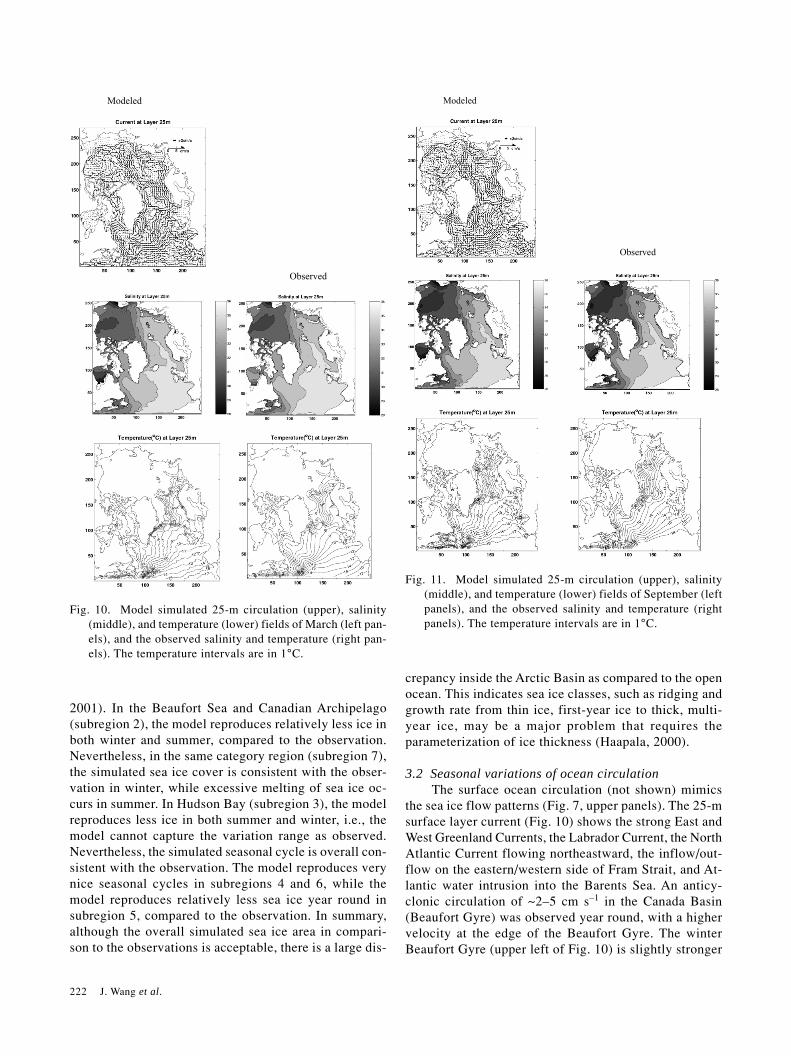
the sea ice flow patterns (Fig. 7, upper panels). The 25-msurface layer current (Fig. 10) shows the strong East andWest Greenland Currents, the Labrador Current, the NorthAtlantic Current flowing northeastward, the inflow/out-flow on the eastern/western side of Fram Strait, and At-lantic water intrusion into the Barents Sea. An anticy-clonic circulation of ~2–5 cm s–1 in the Canada Basin(Beaufort Gyre) was observed year round, with a highervelocity at the edge of the Beaufort Gyre. The winterBeaufort Gyre (upper left of Fig. 10) is slightly stronger
Modeled
Observed
Modeled
Observed
Fig. 10. Model simulated 25-m circulation (upper), salinity(middle), and temperature (lower) fields of March (left pan-els), and the observed salinity and temperature (right pan-els). The temperature intervals are in 1°C.
Fig. 11. Model simulated 25-m circulation (upper), salinity(middle), and temperature (lower) fields of September (leftpanels), and the observed salinity and temperature (rightpanels). The temperature intervals are in 1°C.
A Coupled Ice-Ocean Model in the Pan-Arctic and North Atlantic Ocean: Simulation of Seasonal Cycles 223
than that in summer (upper left of Fig. 11) due to the per-sistent high sea-level pressure system of the Beaufort Highin winter (Fig. 4). In March (upper left of Fig. 10), theTranspolar Drift Stream is stronger than that in summer(upper right of Fig. 11). In both winter and summer (Figs.10 and 11), the model simulated salinity and temperature(left panels) compare reasonably well with the observa-tions (right panels; Steele et al., 2001).
The first remarkable difference between winter andsummer 25-m salinity fields is that there is more fresh-water in summer than winter due to summer melting, bycomparing the freshwater pool in the Canada Basin. Morefreshwater in summer exits via Fram Strait along the EastGreenland Current than in winter. The area of low salin-ity in the Canada Basin is more concentrated in winter(middle panels of Fig. 10) than in summer (middle pan-els of Fig. 11), which indicates a stronger horizontal sa-linity (density) gradient in winter than summer. The dy-
namical mechanism is that the winter anticyclonic windfield produces the anticyclonic surface circulation, whichmaintains freshwater accumulation (or convergence) intothe center of the Canada Basin by a geostropic balance.In summer, because the anticyclonic circulation weakens(Fig. 4, lower), freshwater in the central Canada Basinrelaxes and spreads widely due to the weaker geostrophicbalance (or less convergence). The seasonal cycle of fresh-water accumulation-release process in the Canada Basinis observed from this model simulation. The second fea-ture is that the summer fresh coastal water along the Lab-rador coast is captured compared to the winter, wherethere is ice cover in winter that ejects salt into the upperocean. This feature is consistent with the ice growth ratestudy of Yao et al. (2000).
The 25-m temperature fields show some differencebetween winter and summer. The warm surface Atlanticwater intrudes farther into the eastern Arctic in summer
Modeled
Observed
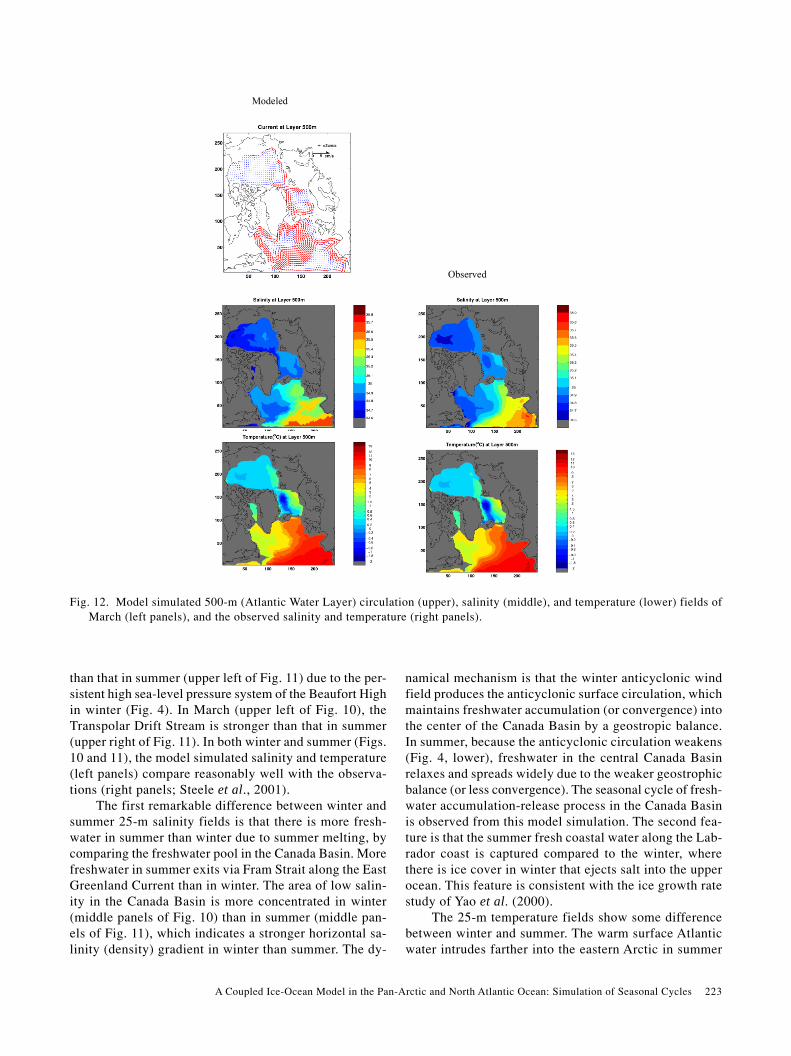
Fig. 12. Model simulated 500-m (Atlantic Water Layer) circulation (upper), salinity (middle), and temperature (lower) fields ofMarch (left panels), and the observed salinity and temperature (right panels).
224 J. Wang et al.
than winter via the Barents Sea, because the warm Atlan-tic Water can maintain its identity of “the warm watermass” in summer while moving northward. In winter, thewarm Atlantic water quickly releases its heat to the at-mosphere while moving northward, such as in the GINSeas and Barents Sea (Ikeda et al., 2001). This is the rea-son that the GIN Seas are the most active regions in termsof air-ice-ocean interactions (Mysak et al., 1990). In theArctic Ocean, the winter temperature is almost homoge-neous horizontally, while the summer temperature fieldindicates warming areas along coast because of open waterconditions there.
At 500 m depth (Fig. 12), the typical Atlantic WaterLayer, the Arctic Basin is dynamically connected to theGIN Seas (Ikeda, 1990) via the Fram Strait, while thenorthern North Atlantic Ocean is disconnected by the Ice-land-Faroe Ridge in the Demark Strait, where dense wa-ter outflow may climb the ridge and flow into the deepocean of the northern Atlantic (Gerdes, 1993). Overall,there is cyclonic circulation in both the Arctic Basin andGIN Seas with a connection via the Fram Strait (Fig. 12,upper panels). In the North Atlantic Ocean, the cycloniccirculation prevails in the Labrador Sea, while anticy-clonic circulation exists in the eastern part. The velocityfield in winter (upper left of Fig. 12) is comparable tothat in summer (not shown) in the North Atlantic Ocean.
There are little seasonal variations in temperature andsalinity at the 500 m depth. The salinity (Fig. 12, middle)
and temperature (Fig. 12, lower) fields in winter havesimilar patterns in summer (not shown). The water massesat the Atlantic Water Layer in the Arctic Ocean indicatethat there exists the same water mass of the Atlantic ori-gin in both the Arctic Basin and GIN Seas with salinityof 34.9–35.1 ppt and a temperature of 0–2°C. The Atlan-tic Water signature can be observed in the eastern GINSeas with salinity of about 35 ppt and temperature of 2–4°C. These features indicate that the Atlantic Water con-tributes significantly to heat balance and salt balance inthe GIN Seas and the Arctic Ocean via its transport andsequentially to the atmosphere-ice-ocean interactions inthe region (Mysak et al., 1990). The simulated salinity(middle, left panel) indicates strong westward diffusionof the Atlantic Layer, compared to the observation (mid-dle, right panel). The model simulates the sustainableAtlantic Layer (lower, left panel), compared to the obser-vation.
The vertically-averaged barotropic current (Fig. 13)indicates the dominance of the cyclonic circulation in theLabrador Sea, the western North Atlantic, and the GINSeas (Clarke et al., 1990), while anticyclonic circulationdominates in the eastern North Atlantic. In the EurasianBasin a strong, elongated cyclonic circulation (Aagaard,1989; Jones et al., 1995) dominates. Topographic veer-ing is the major feature of the transport (Polyakov, 2001).Although the surface current is anticyclonic in the CanadaBasin (Figs. 10 and 11), the overall transport is cyclonic,
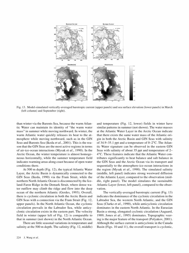
Fig. 13. Model-simulated vertically-averaged barotropic current (upper panels) and sea surface elevation (lower panels) in March(left column) and September (right).
A Coupled Ice-Ocean Model in the Pan-Arctic and North Atlantic Ocean: Simulation of Seasonal Cycles 225
with circulation slightly stronger in winter than in sum-mer (Pfirman et al., 1997). Barotropic current is stronglyrelated to surface elevation (Fig. 13, lower panels). Thegeneral pattern is similar between winter and summer,except that the horizontal gradient in the Canada Basin islarger in winter than in summer because the anticyclonicwind field plays a key role. A high in sea level elevationcorresponds to the Beaufort High in the atmosphere. Asubpolar low exists in the Labrador Sea and a high in theeastern North Atlantic Ocean. The low in the GIN Seasextends to the Eurasian Basin.
To understand the strength of the circulation pattern,the streamfunction or transport was calculated. Table 2shows transports for several major gyres in both Septem-ber and March. The Labrador Gyre has about 28 Sv and26 Sv in winter and summer, respectively, which is un-derestimated because the southern boundary is closed.Ivers (1975) and Reynaud (1994) estimated that the Lab-rador Sea transport is 49–55 Sv using the diagnostic cal-culation, while others estimated that the transport is be-tween 34–37 Sv (Clarke, 1984; Thompson et al., 1986).
In the southern GIN Seas, there is 16 Sv in both sea-
sons, while in the northern GIN Seas winter transport islarger in the winter (14 Sv) than in the summer (12 Sv).In the eastern Arctic (i.e., in Eurasian Basin), there is 17Sv in winter and 16 Sv in summer. In the Canada Basin,there is about 6 Sv in both seasons. In Fram Strait, theoutflow is 10 Sv in winter and 8 Sv in summer. The in-flow via Fram Strait and the Barents Sea Branch is of thesame magnitude, 10 Sv in winter and 8 Sv in summer.There were some field observational estimates based onlimited moorings across Fram Strait. The transports wereestimated ranging from 2 Sv (Polyakov, 2001) to 7 Sv(Aagaard and Greiman, 1975). Zhang et al. (1998) ob-tained 1.9–3.6 Sv using a regional model by prescribingthe inflow and outflow conditions of the same magnitudeat the Denmark Strait. Our estimate may be relativelyhigh. Nevertheless, our model has no prescribed trans-port in the southern open boundary, which is far awayfrom the Arctic. The transport is generated within the pan-Arctic and northern Atlantic Ocean. The only possiblecause for overestimation is due to the sigma-coordinateerror, a weakness of sigma-coordinate models that is dif-ficult to quantify.
Sv Labrador S. GIN N. GIN Eurasian Canada FS-Out FS-Barents-In
Mar. 28 16 14 17 6 10 10Sep. 26 16 12 16 6 8 8
Table 2. Transport (in Sv, 1 Sverdrup = 106 m3s–1) calculated from the model simulation.
Mod
Obs
Summer Winter
Fig. 14. Model-simulated freshwater thickness (upper panels) and climatological freshwater thickness (lower panels) derivedfrom the PHC (Steele et al., 2001) in March (left panels) and September (right panels). The reference salinity is 34.8 ppt.
226 J. Wang et al.
4. Diagnosis Analysis: Freshwater, Heat Content,and Trans-Arctic-Atlantic T and S SectionFreshwater thickness is defined as
FT S S z S z S S zz h
z
= − ( )[ ] − ( ) >=−
=
∑ r r rfor / , ,∆0
0
where Sr is the reference salinity, set to 34.8 ppt (Aagaardand Carmack, 1989), and h is the water depth. Using thisformula, we calculated the winter and summer FT (Fig.14, upper panels), which can be compared to the clima-tology data derived from the observation archives (PHC,Steele et al., 2001) that include the Environmental Work-ing Group (EWG, 1998) data during the 1950s–1980s(Fig. 14 lower panels). Overall, the simulated FT in bothseasons is consistent with the observations (lower pan-els). A large amount of freshwater is accumulated in theBeaufort Gyre in the Canada Basin in both winter andsummer, with the maximum being 17 m in winter and 18m in summer. Note that the 1-m difference is due to theseasonal freezing and melting process, because some offreshwater is stored in the form of sea ice in winter. Thedifference is that winter freshwater in the Beaufort Gyreis confined to the Canada Basin, while in summer, due tothe relaxing wind field (Fig. 4), freshwater is spread in-side the Arctic and out of the Arctic via the Fram Strait tothe East Greenland Current (see lower panels of Fig. 14).The model also simulates similar features (upper panelsof Fig. 14): 1) domain-averaged freshwater is 1-m thicker
in summer (17 m) than in winter with a maximum of 16m, and 2) in summer more freshwater is spread inside theArctic and out of the Arctic Basin via Fram Strait (upperpanels). In addition, the model simulation suggests thatone of the pathways of Arctic freshwater may be con-nected to freshwater in Baffin Bay through the CanadianArchipelago. There are also freshwater reservoirs inBaffin Bay, Hudson Bay (Prinsenberg, 1984), and the Gulfof St. Lawrence, with a maximum of about 10 m (notethat the FT depends on the reference salinity chosen).
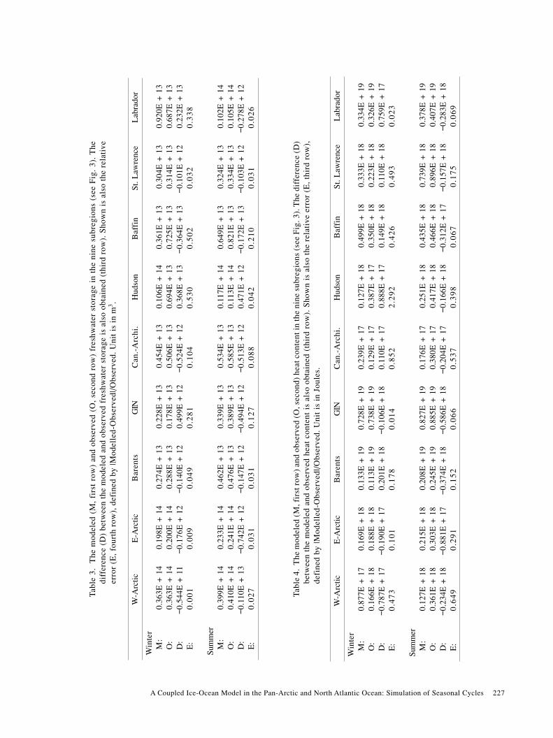
Table 3 demonstrates quantitatively the simulated andobserved freshwater storage in the nine subregions (seeFig. 3 for the subregions). The differences between themodel and observations are calculated and the relativeerrors are also derived for all the subregions. In winter,relative error is low for the western Arctic (0.1%), east-ern Arctic (0.9%), Barents Sea (4.9%), Canadian Archi-pelago (10.4%), and the Gulf of St. Lawrence (3.2%),while relative error is large in GIN Seas (28.1%), Hud-son Bay (53%), Baffin Bay (50.2%), and the LabradorSea (33.8%). In summer, the model captures very well inmost subregions, except in GIN Seas (12.87%) and BaffinBay (21%). This indicates that the model simulates sum-mer freshwater storage better than winter.
Heat content is defined as
HC C T z T zz h
z
= ( ) −[ ]=−
=
∑ ρ P r ∆0
,
Winter Summer
Mod
Obs
Fig. 15. Model-simulated heat content (upper panels) and climatological heat content based on data (lower panels) derived fromthe PHC in March (left panels) and September (right panels).
A Coupled Ice-Ocean Model in the Pan-Arctic and North Atlantic Ocean: Simulation of Seasonal Cycles 227
Tab
le 3
. T
he m
odel
ed (
M,
firs
t ro
w)
and
obse
rved
(O
, se
cond
row
) fr
eshw
ater
sto
rage
in
the
nine
sub
regi
ons
(see
Fig
. 3)
. T
hedi
ffer
ence
(D
) be
twee
n th
e m
odel
ed a
nd o
bser
ved
fres
hwat
er s
tora
ge i
s al
so o
btai
ned
(thi
rd r
ow).
Sho
wn
is a
lso
the
rela
tive
erro
r (E
, fou
rth
row
), d
efin
ed b
y |M
odel
led-
Obs
erve
d|/O
bser
ved.
Uni
t is
in
m3 .
Ta b
le 4
. T
he m
ode l
e d (
M, f
irst
row
) a n
d ob
serv
e d (
O, s
e con
d) h
e at c
onte
nt in
the
nine
sub
regi
ons
(se e
Fig
. 3).
The
dif
fere
nce
(D)
betw
e en
the
mod
e le d
and
obs
e rve
d he
a t c
onte
nt i
s a l
so o
bta i
ned
(thi
rd r
ow).
Sho
wn
is a
lso
the
rela
tive
err
or (
E,
thir
d ro
w),
defi
ned
by |M
ode l
led-
Obs
e rve
d|/O
bse r
ved.
Uni
t is
in
Joul
e s.
W-A
rctic
E-A
rctic
Bar
ents
GIN
Can
.-A
rchi
.H
udso
nB
affi
nSt
. Law
renc
eL
abra
dor
Win
ter
M:
0.36
3E +
14
0.19
8E +
14
0.27
4E +
13
0.22
8E +
13
0.45
4E +
13
0.10
6E +
14
0.36
1E +
13
0.30
4E +
13
0.92
0E +
13
O:
0.36
3E +
14
0.20
0E +
14
0.28
8E +
13
0.17
8E +
13
0.50
6E +
13
0.69
4E +
13
0.72
5E +
13
0.31
4E +
13
0.68
7E +
13
D:
−0.5
44E
+ 1
1−0
.176
E +
12
−0.1
40E
+ 1
20.
499E
+ 1
2−0
.524
E +
12
0.36
8E +
13
−0.3
64E
+ 1
3−0
.101
E +
12
0.23
2E +
13
E:
0.0
01
0.0
09
0.0
49
0.2
81
0.1
04
0.5
30
0.5
02
0.0
32
0.3
38
Sum
mer
M:
0.39
9E +
14
0.23
3E +
14
0.46
2E +
13
0.33
9E +
13
0.53
4E +
13
0.11
7E +
14
0.64
9E +
13
0.32
4E +
13
0.10
2E +
14
O:
0.41
0E +
14
0.24
1E +
14
0.47
6E +
13
0.38
9E +
13
0.58
5E +
13
0.11
3E +
14
0.82
1E +
13
0.33
4E +
13
0.10
5E +
14
D:
−0.1
10E
+ 1
3−0
.742
E +
12
−0.1
47E
+ 1
2−0
.494
E +
12
−0.5
13E
+ 1
20.
471E
+ 1
2−0
.172
E +
13
−0.1
03E
+ 1
2−0
.278
E +
12
E:
0.0
27
0.0
31
0.0
31
0.1
27
0.0
88
0.0
42
0.2
10
0.0
31
0.0
26
W-A
rctic
E-A
rctic
Bar
ents
GIN
Can
.-A
rchi
.H
udso
nB
affi
nSt
. Law
renc
eL
abra
dor
Win
ter
M:
0.87
7E +
17
0.16
9E +
18
0.13
3E +
19
0.72
8E +
19
0.23
9E +
17
0.12
7E +
18
0.49
9E +
18
0.33
3E +
18
0.33
4E +
19
O:
0.16
6E +
18
0.18
8E +
18
0.11
3E +
19
0.73
8E +
19
0.12
9E +
17
0.38
7E +
17
0.35
0E +
18
0.22
3E +
18
0.32
6E +
19
D:
−0.7
87E
+ 1
7−0
.190
E +
17
0.20
1E +
18
−0.1
06E
+ 1
80.
110E
+ 1
70.
888E
+ 1
70.
149E
+ 1
80.
110E
+ 1
80.
759E
+ 1
7E
:0
.47
30
.10
10
.17
80
.01
40
.85
22
.29
20
.42
60
.49
30
.02
3
Sum
mer
M:
0.12
7E +
18
0.21
5E +
18
0.20
8E +
19
0.82
7E +
19
0.17
6E +
17
0.25
1E +
18
0.43
5E +
18
0.73
9E +
18
0.37
8E +
19
O:
0.36
1E +
18
0.30
3E +
18
0.24
5E +
19
0.88
5E +
19
0.38
0E +
17
0.41
7E +
18
0.46
6E +
18
0.89
6E +
18
0.40
7E +
19
D:
−0.2
34E
+ 1
8−0
.881
E +
17
−0.3
74E
+ 1
8−0
.586
E +
18
−0.2
04E
+ 1
7−0
.166
E +
18
−0.3
12E
+ 1
7−0
.157
E +
18
−0.2
83E
+ 1
8E
:0
.64
90
.29
10
.15
20
.06
60
.53
70
.39
80
.06
70
.17
50
.06
9
228 J. Wang et al.
Mod
Obs
a)
b)
Obs.
Obs.
Mod
Mod
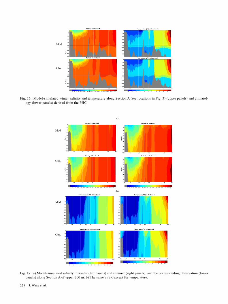
Fig. 16. Model-simulated winter salinity and temperature along Section A (see locations in Fig. 3) (upper panels) and climatol-ogy (lower panels) derived from the PHC.
Fig. 17. a) Model-simulated salinity in winter (left panels) and summer (right panels), and the corresponding observation (lowerpanels) along Section A of upper 200 m. b) The same as a), except for temperature.
A Coupled Ice-Ocean Model in the Pan-Arctic and North Atlantic Ocean: Simulation of Seasonal Cycles 229
where ρ is water density (=1025 kg m–3), CP is specificheat for ocean water (=3903 J kg–1K–1), and Tr is the ref-erence temperature, which is the Atlantic water tempera-ture of 0°C. Using this formula, we calculated heat con-tent from the model simulation (Fig. 15, upper panels)and from the observations (Fig. 15, lower panels) in theupper 1000 m layer.
The observations show that there is more heat trans-port into the Eurasian Basin via the Fram Strait in sum-mer than in winter; the same is so in the Barents Sea (lowerpanels). The reason is that the Atlantic Water loses itsheat to the atmosphere in the GIN Seas on the way to theArctic Ocean. At the same time, the Arctic outflow to-gether with sea ice outflow via the Fram Strait can mixwith the Atlantic Water in the GIN Seas, which cools theAtlantic Water more in winter than in summer. Inside theArctic Ocean, sea ice cover in winter can insulate theoceanic heat flux of the Atlantic Layer from releasing tothe atmosphere. The distribution of heat content tends to
be elongated in the Eurasian Basin in winter, while it tendsto spread westward in summer (right panels). The modelcan reproduce similar patterns for both winter and sum-mer in both spatial distribution and magnitude.
Table 4 shows the comparison between the simulatedand observed heat content in each subregion (see Fig. 3for the subregions). In summer and winter, the model re-produces well heat content in the GIN Seas and in theLabrador Sea. Nevertheless, it does not simulate as wellfor the Barents Sea, eastern Arctic, and it does the worstjob in the western Arctic. The reason is that the simu-lated Atlantic Layer is lower in temperature and thinnerin thickness than the observation toward the western Arc-tic. Large errors exist in the Canadian Archipelago, Hud-son Bay, and the Gulf of St. Lawrence, indicating that theobservations compiled in the PHC dataset may containlarge uncertainty due to sparcity of the measurements.
To reveal the pan-Arctic-Atlantic Ocean T and Sproperties, we constructed the winter T and S sections(Fig. 16) along the pan-Arctic and northern North Atlan-tic Ocean (see locations in Fig. 3). The warm Atlanticwater enters the GIN Seas through the Iceland-FaroeRidge. In the GIN Seas, the warm Atlantic Water main-tains its original identity, although somewhat cooled.
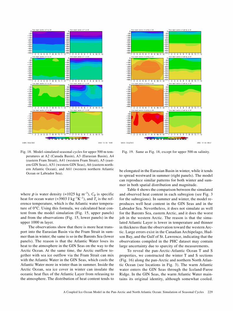
Fig. 19. Same as Fig. 18, except for upper 500-m salinity.Fig. 18. Model-simulated seasonal cycles for upper 500 m tem-peratures at A2 (Canada Basin), A3 (Eurasian Basin), A4(eastern Fram Strait), A41 (western Fram Strait), A5 (east-ern GIN Seas), A51 (western GIN Seas), A6 (eastern north-ern Atlantic Ocean), and A61 (western northern AtlanticOcean or Labrador Sea).
230 J. Wang et al.
However, as it enters the Eurasian Basin, its surface layeris further cooled, deepened, and modified by the coldArctic Surface Water. In the Arctic Ocean, the subsurfaceAtlantic Water continues deepening westward, approach-ing the coldest water in the Bering Strait (Fig. 16, rightpanels).
Similarly, the saline North Atlantic Water intrudesthe GIN Seas over the Iceland-Faroe Ridge (Fig. 16, leftpanels). As the Atlantic Water continues moving towardthe Arctic, it deepens toward the west. The Arctic Sur-face Water is fresher in the west than the east, due to theintrusion of the saline Atlantic Water. Nevertheless, sa-linity in the deep layer is comparable in the Canada, Si-berian, and Eurasian Basins. One important feature is thatin the central GIN Seas, saline, warm water penetratesdown to about the 500-m depth captured by the model,which indicates a possible deep convection in the regionduring winter. Thus, the central and eastern GIN Seas arevery likely unstable for convection in response to atmos-pheric forcing. The simulated salinity and temperature(upper panels) are comparable to the observations (lowerpanels). However, the simulated Atlantic Layer is thin-ner than the observation, possibly due to strong modeldiffusion.
To further describe the detailed features of sectionA, we examine the upper 200 m salinity (Fig. 17(a)) andtemperature (Fig. 17(b)). The surface layer is relativelysaline in winter (left panels of Fig. 17(a)) compared tothe freshening in summer (right panels of Fig. 17(a)),particularly in the western and central Arctic. In the GINSeas, the freshening in the upper layer (right panels ofFig. 17(a)) may inhibit convection in summer, while inwinter the ambient saline precondition may trigger a deepconvection down to a depth of 500 m (left panels of Fig.17(a)). The temperature sections (Fig. 17(b)) also revealpossible deep convection in the GIN Seas in winter (leftpanels of Fig. 17(b)), compared to summer (right panelsof Fig. 17(b)).
To examine seasonal cycles of temperature and sa-linity at different locations, we selected several repre-sentative regions along Section A (see the locations inFig. 3): A2 (Canada Basin), A3 (Eurasian Basin), A4 (east-ern Fram Strait), A5 (eastern GIN Seas), and A6 (easternnorthern North Atlantic) with the inflow conditions. Sta-tions A41 (western Fram Strait, near D1), A51 (westernGIN Seas, parallel to A5), and A61 (northern LabradorSea) are selected for comparison with the outflow condi-tions. Figures 18 and 19 show the seasonal cycles of dif-ferent locations for temperature and salinity, respectively.In the Canada Basin (A2), the surface layer experiencesseasonal variations in both temperature and salinity. Inthe Eurasian Basin (A3), the surface layer temperaturehas less variation (Fig. 18); however, there is less salineAtlantic Water intrusion during summer (July–October),
and significant freshening occurs in summer (Fig. 19). Inthe eastern Fram Strait (A4), strong seasonal variationsof T and S occur in both the surface layer and the Atlan-tic Layer. The intrusion of the surface warm Atlantic Wateris modified when it enters the Fram Strait in winter, whileit retains its warm identity in summer (Fig. 18). The sa-line surface Atlantic Water mixes with the Arctic outflowyear-round with a maximum in May. By contrast, in west-ern Fram Strait (A41), cold surface water remains year-round (Fig. 18), and more fresh water outflow occurs insummer and fall (Fig. 19).
In the eastern GIN Seas (A5), Atlantic Water domi-nates with seasonal warming and cooling (Fig. 18), whilesurface salinity has strong seasonal variation (Fig. 19).Particularly interesting is that deep convection may oc-cur from March to April (Clarke et al., 1990; Hakkinenet al., 1992), because the surface salinity becomes asdense as the Atlantic intermediate water. In the westernGIN Seas (A51), strong seasonal variation occurs in bothtemperature and salinity with interactions between Arc-tic surface water outflow and the Atlantic Water. Althoughsurface salinity may become dense in winter, it onlyreaches to about 100 m, indicating that the deep convec-tion may not likely occur in the western GIN Seas.
In the northern North Atlantic Ocean, there are sig-nificant differences between the eastern part (A6) andwestern part (A61, Labrador Sea). In the Labrador Sea,surface freshening exits year-round, while the tempera-ture profile has a feature similar to upstream station A51.
5. Conclusions and DiscussionThe development and application of the CIOM have
been described. It is encouraging that CIOM reproducesmany of the dynamical and thermodynamical features ofthe Arctic ice-ocean system. Based on the investigationin precious sections, results can be summarized as fol-lows.
1) The surface ice circulation is anticyclonic in theCanada Basin, with a stonger magnitude in winter than insummer. Sea ice thickness distribution is reasonably re-produced, with thick ice located at the northern Green-land and the Canadian Archipelago. This is qualitativelyconsistent with available observations based on limitedfield measurements. The model-simulated sea ice concen-tration distributions in both seasons are also consistentwith available climatology.
2) The model reproduces the ice cover in the Arc-tic Ocean as a whole reasonably well. Nevertheless, themodel has better performance in the open oceans, such asthe Labrador Sea, GIN Seas, and the Barents Sea, thanthe mediterranean Arctic Ocean, where sea ice rangesfrom first-year ice to multi-year ice, and the thicknessdistribution is more complicated than that in the openocean. Thus, sea ice distribution for describing thickness
A Coupled Ice-Ocean Model in the Pan-Arctic and North Atlantic Ocean: Simulation of Seasonal Cycles 231
features should be applied in the near future.3) The surface ocean circulation in the Canada
Basin is anticyclonic in both seasons. The low salinityarea tends to converge in the Canada Basin in winter com-pared to less convergence in summer due to stronger anti-cyclonic circulation in winter than summer.
4) At 500 m depth, the typical Atlantic Layer, thesimulated ocean circulation patterns in the Labrador Sea,the GIN Seas, the Eurasian Basin and the Canada Basinare cyclonic. Temperature and salinity have little seasonalvariation at this layer in the Artic Ocean.
5) The seasonal transports of major basins are ob-tained, although these numbers need further observationsto confirm. The model estimate of the Fram Strait trans-port of 10 Sv in winter and 8 Sv in summer may be at thehigh end compared to 7 Sv observed by Aagaard andGreiman (1975). Nevertheless, a transport as high as 10–15 Sv was observed (Schauer and Fahrbach, 2004). Thisis an open question to be further investigated.
6) Model-simulated freshwater distribution com-pares well with the observations, which was confined inthe Canada Basin. Freshwater in the Canada Basin tendsto converge in winter compared to summer because anti-cyclonic wind stress and ocean circulation there relaxes(becomes relatively weak) in summer. Thus, extensivefreshwater in liquid form is exported out of the ArcticOcean in summer compared to winter. The model-simu-lated heat content is also consistent with the observationin spatial distribution and in magnitude.
7) Based on Section A, we observed the intrusionof the Atlantic Water into the Arctic Ocean. The Atlanticsurface water character is gradually modified on its wayto the Arctic, while the Atlantic Water from 300–1000 mretains its original characters. In the GIN Seas, deep con-vection more likely occurs in winter than in summer, be-cause summer freshening occurs at the ocean surface thatstabilizes the water column. Seasonal cycles of tempera-ture and salinity at several selected locations reveal re-gional features in the ice-ocean interactions. More model-data comparisons are necessary for further understand-ing the regional features of dynamics and thermodynam-ics.
This modeling exercise can be extended to study1) interannual variability of the Arctic and North Atlan-tic Ocean circulation, Atlantic Water intrusion and its ef-fects on the Arctic halocline and surface water (Steeleand Boyd, 1998), and sea ice distribution (Wang et al.,2005); 2) the relationship of the Arctic Oscillation andthe Atlantic Water intrusion (Wang et al., 2004); 3) fresh-water and heat budget in the changing Arctic Ocean; and4) parameterization of sea ice thickness distribution andimprovement of the representation of sea ice thicknessesof different types, from first-year ice to multi-year ice(Haapala, 2000).
AcknowledgementsWe appreciate financial support partly from the Fron-
tier Research Center for Global Change (FRCGC),through JAMSTEC, Japan to International Arctic Re-search Center, partly from the Coastal Marine Institute/Minerals Management Service, and partly from the De-partment of Fisheries Oceans, Canada. We also appreci-ate fruitful discussions with Drs. T. Yao, C. Tang, J. Walsh,A. Proshutinsky, I. Polyakov, and B. Wu. The first authorthanks Drs. Tom Yao and Charles Tang of the BedfordInstitute of Oceanography for the collaborative develop-ment of this model in the Labrador Sea.
ReferencesAagaard, K. (1981): On the deep circulation in the Arctic Ocean.
Deep-Sea Res., 28A, 251–268.Aagaard, K. (1989): A synthesis of the Arctic Ocean circula-
tion. Rapp. P.V. Reun. Cons. Int. Explor. Mer., 188, 11–22.Aagaard, K. and E. C. Carmack (1989): The role of sea ice and
other fresh water in the Arctic circulation. J. Geophys. Res.,94, 14,485–14,498.
Aagaard, K. and P. Greiman (1975): Toward new mass and heatbudgets for the Arctic mediterranean seas. J. Geophys. Res.,80, 3821–3827.
Blumberg, A. F. and G. L. Mellor (1987): A description of 3-Dcoastal ocean circulation model. p 1–16. In Coastal andEsturine Sciences 4: 3-D Coastal Ocean Models, ed. by N.S. Heaps, American Geophysical Union, Washington, D.C.
Bourke, R. H. and R. P. Garrett (1987): Sea ice thickness dis-tribution in the Arctic Ocean. Cold Regions Science andTechnology, 13, 259–280.
Cheng, A. and R. Preller (1992): An ice-ocean coupled modelfor the Northern Hemisphere. Geophys. Res. Lett., 19, 901–904.
Clarke, R. A. (1984): Transport through the Cape Farewell-Femish Cap section. Rapp. P.V. Reu. Cos. Int. Explor. Mer.,185, 120–130.
Clarke, R. A., J. H. Swift, J. L. Reid and K. P. Koltermann(1990): The formation of Greenland Sea Deep Water: dou-ble diffusion or deep convection? Deep-Sea Res., 37, 1385–1424.
Coachman, L. K. and K. Aagaard (1974): Physical oceanogra-phy of arctic and subarctic seas. In Marine Geology andOceanography of the Arctic Seas, Chap. 1, ed. by Y. Herman,Springer-Verlag.
Dunbar, M. and W. Wittmann (1963): Some features of icemovement in the Arctic Basin. p. 90–108. In Proceedingsof Arctic Basin Symposium 1962, Arctic Institute of NorthAmerica, Washington, D.C.
Environmental Working Group (EWG) (1998): National Snowand Ice Data Center, University of Colorado.
Fleming, G. H. and A. J. Semtner, Jr. (1991): A numerical studyof interannual ocean forcing on Arctic ice. J. Geophys. Res.,96, 4589–4603.
Gerdes, R. (1993): A primitive equation ocean circulation modelusing a general vertical coordinate transformation. II. Ap-plication to an overflow problem. J. Geophys. Res., 98,14,703–14,726.
232 J. Wang et al.
Gloersen, P., W. J. Campbell, D. J. Cavalieri, J. C. Comiso, C.L. Parkinson and H. J. Zwally (1992): Arctic and AntarcticSea Ice, 1978–1987: Satellite passive-microwave observa-tions and analysis. NASA SP-511, Washington, D.C., 290pp.
Haapala, J. (2000): On the modelling of ice-thickness redistri-bution. J. Glaciology, 46, 427–437.
Hakkinen, S. (2000): Simulated low-frequency modes of cir-culation in the Arctic Ocean. J. Geophys. Res., 105, 6549–6564.
Hakkinen, S., G. L. Mellor and L. H. Kantha (1992): Modelingdeep convection in the Greenland Sea. J. Geophys. Res.,97, 5389–5408.
Haney, R. L. (1991): On the pressure gradient force over steeptopography in sigma coordinate ocean models. J. Phys.Oceanogr., 21, 610–619.
Hibler, W. D., III (1979): A dynamic thermodynamic sea icemodel. J. Phys. Oceanogr., 9, 815–846.
Hibler, W. D., III (1980): Modeling a variable thickness sea icecover. Mon. Wea. Rev., 108, 1943–1973.
Hibler, W. D., III and K. Bryan (1987): A diognostic ice-oceanmodel. J. Phys. Oceanogr., 17, 987–1015.
Holland, M. M., C. M. Bitz, M. Eby and A. J. Weaver (2001):The role of ice-ocean interactions in the variability of theNorth Atlantic thermohaline circulation. J. Climate, 14,656–675.
Hunke, E. C. and J. K. Dukowicz (1997): An elastic-viscous-plastic model for sea ice dynamics. J. Phys. Oceanogr., 27,1849–1867.
Hurrell, J. W. and H. van Loon (1997): Decadal variations inclimate associated with the North Atlantic Oscillation. Cli-mate Change, 36, 301–326.
Ikeda, M. (1990): Decadal oscillation of the air-ice-sea systemin the northern hemisphere. Atmosphere-Ocean, 28, 106–139.
Ikeda, M., J. Wang and J.-P. Zhao (2001): Hypersensitivedecadal oscillation in the Arctic/subarctic climate. Geophys.Res. Lett., 28, 1275–1278.
Ivers, W. D. (1975): The deep circulation in the northern At-lantic with special reference to the Labrador Sea. Ph.D.Thesis, University of California at San Diego, 179 pp.
Jones, E. P., B. Rudels and L. G. Anderson (1995): Deep wa-ters of the Arctic Ocean: origins and circulation. Deep-SeaRes., 42, 737–760.
Kantha, L. H. and G. L. Mellor (1989): Application of a two-dimensional coupled ocean-ice model to the Bering Seamarginal ice zone. J. Geophys. Res., 94, 10,921–10,936.
Karcher, M., J. Brauch, B. Fritzsch, R. Gerdes, F. Kauker, C.Köberle and M. Prange (1999): Variability in the Nordicseas exchange-model results 1979–1993. ICES CM, 1999,L: 18.
Kimura, N. and M. Wakatsuchi (2000): Relationship betweensea-ice motion and geostrophic wind in the northern hemi-sphere. Geophys. Res. Lett., 27, 3735–3738.
Köberle, C. and R. Gerdes (2003): Mechanisms determiningthe variability of Arctic sea ice conditions and export. J.Climate, 16, 2843–2858.
Maslowski, W., D. C. Marble, W. Walczowski and A. J. Semtner(2001): On larger-scale shifts in the Arctic Ocean and sea-
ice conditions during 1979–98. Annuals. of Glaciol., 33,545–550.
Mellor, G. L. and L. H. Kantha (1989): An ice-ocean coupledmodel. J. Geophys. Res., 94, 10,937–10,954.
Mellor, G. L., T. Ezer and L.-Y. Oey (1994): The pressure gra-dient conundrum of sigma coordinate ocean models. J.Atmos. Oceanic Technol., 11, 1126–1134.
Mysak, L. A. and J. Wang (1991): Climatic atlas of seasonaland annual Arctic sea-level pressure, SLP anomalies andsea-ice concentration, 1953–88. C2GCR Report No. 91-14,McGill Univ., Montreal, 194 pp.
Mysak, L. A., D. K. Manak and R. F. Marsden (1990): Sea-iceanomalies observed in the Greenland and Labrador Seasduring 1901–1984 and their relation to an interdecadal Arc-tic climate cycle. Climate Dynamics, 5, 111–133.
Oberhuber, J. M. (1993): Simulation of the Atlantic circulationwith a coupled sea-ice-mixed layer-isopycnal general cir-culation model. Part I: Model description. J. Phys.Oceanogr., 23, 808–829.
Parkinson, C. L., D. J. Cavalieri, P. Gloersen, H. J. Zwally andJ. C. Comiso (1999): Arctic sea ice extents, areas, and trends,1978–1996. J. Geophys. Res., 104, 20,837–20,856.
Pfirman, S. L., R. Colony, D. Nunberg, H. Eicken and R. Rigor(1997): Reconstructing the origin and trajectory of driftingArctic sea ice. J. Geophys. Res., 102, 12,575–12,586.
Polyakov, I. (2001): An eddy parameterization based on maxi-mum entropy production with application to modelling theArctic Ocean circulation. J. Phys. Oceanogr., 31, 2255–2270.
Prinsenberg, S. J. (1984): Freshwater contents and heat budg-ets of James Bay and Hudson Bay. Cont. Shelf Res., 3, 191–200.
Proshutinsky, A. and 14 others (2001): Multinational effort stud-ies differences among Arctic ocean models. EOS, AGU,82(51), 637–644.
Reynaud, T. H. (1994): Dynamics of the Northwestern AtlanticOcean: A diagnostic study. Ph.D. Thesis (also C2 GCR Rep.No. 94-5), McGill University, Montreal, 267 pp.
Rigor, I. G., J. M. Wallace and R. L. Colony (2002): Responseof sea ice to the Arctic Oscillation. J. Climate, 15, 2648–2663.
Saenko, O. A., G. M. Flato and A. J. Weaver (2002): Improvedrepresentation of sea-ice processes in climate models.Atmos-Oceans, 40, 21–43.
Saucier, F. J., F. Roy, D. Gilbert, P. Pellerin and H. Ritchie(2003): The formation and circulation processes of watermasses in the Gulf of St. Lawrence. J. Geophys. Res., 108,3269–3289.
Schauer, U. and E. Fahrbach (2004): Arctic warming throughthe Fram Strait: Ocean heat transport from 3 years of meas-urements. J. Geophys. Res., 109, C06026, doi:10.1029/2003JC001823.
Semtner, A. J., Jr. (1976): Numerical simulation of the ArcticOcean circulation. J. Phys. Oceanogr., 6, 409–424.
Steele, M. and T. Boyd (1998): Retreat of the cold haloclinelayer in the Arctic Ocean. J. Geophys. Res., 103, 10,419–10,435.
Steele, M., R. Rebecca and W. Ermold (2001): PHC: A globalocean hydrography with a high-quality Arctic Ocean. J.
A Coupled Ice-Ocean Model in the Pan-Arctic and North Atlantic Ocean: Simulation of Seasonal Cycles 233
Climate, 14, 2079–2087.Thompson, K. R., J. R. N. Lazier and B. Taylor (1986): Wind-
forced changes in Labrador Current transport. J. Geophys.Res., 91, 14,261–14,268.
Thorndike, A. S., D. A. Rothrock, G. A. Maykut and R. Colony(1975): The thickness of distribution of sea ice, J. Geophys.Res., 80, 4501–4513.
van Loon, H. and J. C. Rogers (1978): The seesaw in wintertemperature between Greenland and northern Europe, Part1: General description. Mon. Wea. Rev., 106, 296–310.
Wang, J. (2001): A nowcast/forecast system for coastal oceancirculation (NFSCOC) with a simple nudging data assimi-lation. J. Atmos. Oceanic Technol., 18, 1037–1047.
Wang, J. and M. Ikeda (2001): Arctic Sea-Ice Oscillation: Re-gional and seasonal perspectives. Annals of Glaciology, 33,481–492.
Wang, J., L. A. Mysak and R. G. Ingram (1994a): A numericalsimulation of sea-ice cover in Hudson Bay. J. Phys.Oceanogr., 24, 2515–2533.
Wang, J., L. A. Mysak and R. G. Ingram (1994b): Interannualvariability of sea-ice cover in Hudson Bay, Baffin Bay andthe Labrador Sea. Atmosphere-Ocean, 32(2), 421–447.
Wang, J., M. Jin, V. Patrick, J. Allen, D. Eslinger, C. Mooersand T. Cooney (2001): Numerical simulation of the seasonalocean circulation patterns and thermohaline structure ofPrince William Sound, Alaska. Fisheries Oceanogr., 10(Suppl. 1), 132–148.
Wang, J., Q. Liu and M. Jin (2002): A User’s Guide for a Cou-
pled Ice-Ocean Model (CIOM) in the Pan-Arctic and NorthAtlantic Oceans. International Arctic Research Center-Fron-tier Research System for Global Change, Tech. Rep. 02-01,65 pp.
Wang, J., B. Wu, C. L. Tang, J. E. Walsh and M. Ikeda (2004):Seesaw structure of subsurface temperature anomalies be-tween the Barents Sea and the Labrador Sea. Geophys. Res.Lett., 31, L19301, doi:10.1029/2004GL019981.
Wang, J., M. Ikeda, S. Zhang and G. Gerdes (2005): Linkingthe northern hemisphere sea ice reduction trend and thequasi-decadal Arctic sea ice oscillation. Climate Dyn., 1432-0894 (on line), DOI:10.1007/s00382-004-0454-5.
Weatherly, J. W. and J. E. Walsh (1996): The effects of precipi-tation and river runoff in a coupled ice-ocean model of theArctic. Climate Dyn., 12, 785–798.
Yao, T., C. L. Tang and I. K. Peterson (2000): Modeling theseasonal variation of sea ice in the Labrador Sea with a cou-pled multicategory ice model and the Princeton oceanmodel. J. Geophys. Res., 105, 1153–1165.
Zhang, J., B. Hibler, M. Steele and A. D. Rothrock (1998): Arcticice-ocean modeling with and without climate restoring. J.Phys. Oceanogr., 28, 191–217.
Zhang, J., A. D. Rothrock and M. Steele (2000): Recent changesin Arctic sea ice: the interplay between ice dynamics andthermodynamics. J. Climate, 13, 3099–3114.
Zhang, X. and J. Zhang (2001): Heat and freshwater budgetand pathways in the Arctic Mediterranean in a coupledocean/sea-ice model. J. Oceanogr., 57, 207–234.