A Coupled Phasic Exchange Algorithm for Three-Dimensional Multi-Field Analysis of Heated Flows with Mass Transfer

Robert F. Kunz, Brett W. Siebert, W. Kevin Cope, Norman F. Foster, Steven P. Antal, Stephen M. Ettorre

Lockheed-Martin, Schenectady, NY

ABSTRACT

A three-dimensional multi-field Coupled Phasic Exchange (CPE) algorithm, for the prediction of general two-phase flows is presented. The algorithm is applicable to an arbitrary number of fields - a four-field construct is adopted here. Ensemble averaged transport equations for mass, momentum, energy and turbulence transport are solved for each field (continuous liquid, continuous vapor, dis-perse liquid, disperse vapor). This four field structure allows for analysis of adiabatic and boiling sys-tems which contain flow regimes from bubbly through annular. Interfacial mass, momentum, turbulence and heat transfer models provide coupling between fields. The CPE algorithm is a semi-coupled implicit method to solve the set of 25 equations which arise in the formulation. In this paper, the CPE algorithm is summarized, with emphasis on six component numerical strategies employed in the method. These are: 1) Incorporation of interfacial momentum force terms in the control volume face flux reconstruction. 2) Coupled solution of the discrete linearized system of four constituent field equations for each transport scalar. 3) A consistent pressure-velocity correction scheme which prop-erly accounts for drag and mass transfer. 4) An additive correction strategy for efficient solution of the mixture continuity and coupled field continuity equations. 5) An implicit source term treatment for volume fraction equations which ensures realizability of volume fraction fields during the course of iteration. 6) Coupling of the phasic continuity and compatibility equations within the framework of a pressure-volume fraction-velocity correction scheme. The necessity/effectiveness of these strategies is demonstrated in applications to several test cases. The effectiveness and accuracy of the overall method is demonstrated using results of a three-dimensional analysis of boiling SUVA flow in a verti-cal coolant passage element.

KEYWORDS:

Computational Fluid Dynamics (CFD), multi-field, multi-dimensional, boiling heat exchanger

1

NOMENCLATURE

Ak, Bk, Dk Velocity pressure couplingcoefficients

AP, Aj Influence coefficientsA, N, S, E, W, T, B, U, L, D, P

Coefficient and iteration matrixcomponents

α Volume fraction

bkl Interface exchange termC1, C2 k-ε model constantsCTD Turbulence dispersion force

constantDH Hydraulic diameter of geometry

Drag force coefficientδxx, δyy, δzz Second order accurate central

second difference operatorsTurbulent dissipation rate

Fk, Fε Drag coefficient multiplier for k, εequations.

φ General transport scalarφx, φy, φz Nondimensional wave numbersgi Gravity vector

Γkl Mass transfer rate from field k to field l

h Enthalpy

Hkl Interfacial heat transfer coefficient

k Turbulent kinetic energykx, ky, kz Wave numbersL Length of geometry

Continuity errorNon-drag interfacial force onfield k arising from interfacewith field l

µt Turbulent viscosityBoundary normal vector

ni, nj, nk Number of nodes in each directionNφ, NN Number of fields, nodes presentω Underrelaxation factor,

weighting factor for Jacobi scheme

Pk Production of turbulence energyPrt, Prk, Prε Turbulent Prandtl numbers

Pk, Sk, Rk, Ck Coefficients in pressure-volume

fraction correction equationp Pressure

Qk Wall and volumetric heat transferrate to field k

Re Reynolds numberρ DensityS General source termT Temperatureui Cartesian velocity componentV Cell volumexi Cartesian coordinate

Subscripts, Superscripts

‘ Correction quantity* Quantity available after

momentum equation solution^ Quantity available after single

iterative sweep

Amplitude of quantity Fouriertransformed in x

Amplitude of quantity Fouriertransformed in x and y

ijk Node counterk, l Field indicatorsl, m Fourier mode indicesn, n+1 Previous and current iterationNφ, NN Number of fields, nodes presentP, N, S, E, W, T, B

Point, neighbor node indicatorsn, s, e, w, t, b Neighbor face indicatorsi, j Cartesian tensor indicesint Value at interface between field

paircl, cv, dl, dv Four field indicatorsc, d Continuous, disperse field

indicators

Dlk

ε

m·*

Milk

n

2

INTRODUCTION

In many industrial multi-phase flow environments, nonequilibrium dynamics and thermody-namics at the interfaces between component phases play important roles in determining instantaneous volume fraction, velocity and temperature distributions within the flow. For this reason, resolving and/or modelling interfacial physics is required for the analysis of the thermal-hydraulic performance of many multi-phase devices. Direct simulation of the instantaneous flow field will not be practical for engineering analyses of complex multi-component flow fields for decades. Accordingly, many groups have employed volume or ensemble averaged governing equations, where the instantaneous physics associated with the interface are averaged away (Ishii (1975), Carver and Salcudean (1986), Lahey (1996), for example). In these approaches, closure must be provided for correlations of fluctu-ating quantities which appear in the averaged equations. In flows where different regimes can simul-taneously exist (say bubbly, churn turbulent, annular), multiple interface types can exist between a given phase pair. In these circumstances, an approach which employs multiple fields (i.e., Nφ > 2) is forthcoming. This is because distinct physical processes associated with the interface between the same phase pair (e.g., drag between bubbles and continuous liquid vs. drag between droplets and con-tinuous vapor) can be more directly identified with exact terms in the averaged equations, and mod-elled accordingly. In boiling heat exchanger applications, a four-field model which incorporates continuous liquid, continuous vapor, disperse liquid and disperse vapor, represents a useful compro-mise between model sophistication and computer resource requirements. The four-field modelling approach has been deployed successfully by several researchers including Kelly (1993) and Siebert et al. (1995).

In this paper, a new multi-field algorithm for computing boiling two-phase flows in heat exchangers is presented. Though the algorithm is generally applicable to an arbitrary number of fields, the authors have adopted a four-field construct. Ensemble averaged equations for mass, momentum, energy and turbulence transport are solved for each of these four fields (continuous liq-uid, continuous vapor, disperse liquid, disperse vapor). In three dimensions, 24 coupled partial differ-ential equations, and a compatibility condition (Σαk = 1), arise in the formulation. Interfacial mass, momentum, turbulence and heat transfer models provide physical coupling between fields. Approxi-mately thirty models for these exchange processes appear. Additionally, models for boiling heat trans-fer mechanisms are required. This four field structure allows for analysis of adiabatic and boiling systems which contain flow regimes from bubbly through annular. A summary of the physical models employed is provided in Siebert et al. (1995).

In addition to the physical modelling complexities which arise when a four-field approach is pursued, the numerical simulation of the complete four-field system is a formidable task. Many issues arise, including variable coupling, high geometric aspect ratios, discretization of modelled terms and well-posedness of the modelled system. The focus of this paper is on progress the authors have made in developing a new algorithm for the robust and efficient solution of general multi-phase flows, in the context of a four-field model with mass transfer.

In the four-field construct, full coupling of the governing equations in two and three dimen-sions, within the framework of an approximate Newton scheme, can be impractical, due principally to the size of the Jacobian matrices which arise when such a formulation is adopted. Also, arbitrarily maximizing variable coupling gives rise to a less versatile development platform and, for some multi-component systems, can give rise to instability of a time marching or relaxation scheme (Stewart and

3

4

Wendroff (1984), Kunz et al. (1997) for example). Accordingly, the authors have adopted a memory efficient and easily adaptable segregated pressure-based scheme as a baseline numerical platform. Coupling between the four fields is accomplished via the Coupled Phasic Exchange (CPE) algorithm presented here. In this paper, six component numerical strategies employed in the method are summa-rized. These are: 1) Incorporation of interfacial momentum force terms in the control volume face flux reconstruction. 2) Coupled solution of the discrete linearized system of constituent field equa-tions for each transport scalar. 3) A consistent pressure-velocity correction scheme which properly accounts for drag and mass transfer. 4) An additive correction strategy for efficient solution of the mixture continuity and coupled field continuity equations. 5) An implicit source term treatment for volume fraction equations which ensures realizability of volume fraction fields during the course of iteration. 6) Coupling of the phasic continuity and compatibility equations within the framework of a pressure-volume fraction-velocity correction scheme.

The paper is organized as follows. A brief summary of the governing equations and baseline (single phase) numerics is first given. Each of the six algorithmic components of the CPE algorithm are then described. Stability analyses, convergence histories and sample results for several two-dimensional and three-dimensional test cases are used to demonstrate the theory behind and effective-ness of the numerics. Finally, results of a three-dimensional analysis of a boiling SUVA flow in a ver-tical coolant passage element are presented. Comparison with local volume fraction and pressure drop data are provided which demonstrate the accuracy of the method in realistic design applications.

BASELINE FORMULATION

Governing Equations

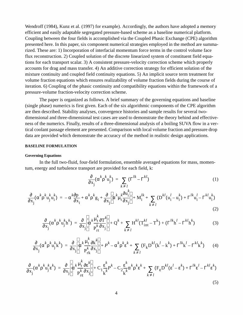
In the full two-fluid, four-field formulation, ensemble averaged equations for mass, momen-tum, energy and turbulence transport are provided for each field, k:

(1)

(2)

(3)

(4)

(5)

xj∂∂ αkρk

ujk( ) Γ lk Γkl

–( )k l≠∑=

xj∂∂ αkρk

ujkui

k( ) αk

xi∂∂p αkρk

gi xj∂∂ αkµt

k

xj∂∂ui

k

++– Milk

Dkl

uil

uik

–( ) Γ lkui

l Γklui

k–+( )

k l≠∑+ +=

xj∂∂ αkρk

ujkh

k( )xj∂∂ αk µt

k

Prtk

------xj∂

∂Tk

Qk

Hkl

Tintkl

Tk

–( ) Γ lkh

l Γklh

k–( )+

k l≠∑+ +=

xj∂∂ αkρk

ujkk

k( )xj∂∂ αk µt

k

Prkk

--------xj∂

∂kk

Pk

+ αkρkεk– FkD

klk

lk

k–( ) Γ lk

kl Γkl

kk

–+( )k l≠∑+=

xj∂∂ αkρk

ujkεk( )

xj∂∂ αk µt

k

Prεk

-------xj∂

∂εk

C1εk

kk

-----Pk

C2εk

kk

-----αkρkεk– FεD

kl εl εk–( ) Γ lkεl Γklεk

–+( )k l≠∑+ +=

The four-fields, k, accounted for are continuous liquid, continuous vapor, disperse liquid and disperse vapor (hereafter cl, cv, dl, dv). Considering, for the present discussion, flows for which each component field’s density is constant, closure of equations 1 through 5 is achieved through specifica-tion of drag and non-drag interfacial force models, , , interfacial heat trans-fer and mass transfer models, , apportioned wall and volumetric heating rates, Qk, and turbulence model parameters. A high Reynolds number k-ε model, modified to include additional interfacial production, drag and mass transfer rate terms, is employed for the two continuous fields. In three dimensions, the four field system adopted employs 24 discrete transport equations plus a com-patibility constraint for the 25 unknowns (4(ui

k + hk + αk) + 2(kk + k) + p).

Baseline Numerics

For single phase flow, the algorithm utilized follows established segregated pressure based methodology and is briefly summarized here: The governing equations are cast in generalized coordi-nates and a lagged coefficient linearization is applied (Clift and Forsyth (1994) for example). A colo-cated variable arrangement is used on block structured grids. One of several diagonal dominance preserving, finite volume spatial discretization schemes is selected for the momentum, enthalpy and turbulence transport equations giving rise to discrete equations of the form:

(6)

Continuity is introduced through a pressure correction equation, based on the SIMPLEC algo-rithm (Van Doormal and Raithby (1984)). In constructing cell face fluxes, a momentum interpolation scheme due to Rhie and Chow (1983) is employed which introduces damping in the continuity equa-tion. At each iteration, the discrete momentum equations are solved approximately, followed by a more exact solution of the pressure correction equation. Enthalpy and turbulence scalars are then solved in succession.

CPE SCHEME

The momentum, energy and turbulence equations for individual constituent fields (equations 2-5) contain significantly more terms than those which arise in single phase or homogeneous mixture applications. In the boiling heat exchanger systems of interest to the authors, the additional terms which arise are due to buoyancy, mass transfer, external heat sources and a rich set of models for var-ious interfacial dynamics. The significant inter-field coupling which these sources introduce can be accommodated within the numerics in several ways:

First, the solution of the linearized system of equations which appear for each transport scalar can be carried out implicitly after proper linearization of the inter-field transfer terms. Indeed, the need for such improved field coupling at the scalar solver level is what motivated the Partial Elimina-tion Algorithm (PEA) of Spalding (1980) and the SINCE Algorithm of Lo (1990). The present CPE method incorporates field coupling at the linear solver level in the spirit of these approaches, but, as described below, is more efficient, more implicit and easily generalized to an arbitrary number of fields.

Second, the pressure-velocity coupling which is used can be constructed to contain much of the richness of the interfield transfer terms which appear in the momentum equations. Indeed, in ear-lier work by the present authors (Siebert and Antal (1993)), it was found that derivation of a mixture

Dlk

Dkl

= Milk

- Mikl

=H

kl Γkl,

ε

APk φP

kAj

kφjk

j=NSEWTB∑ S

k+=

5

pressure corrector which accommodates interfield coupling due to drag and mass transfer could improve the robustness of a pressure based scheme. As mentioned above, in colocated grid algo-rithms, pressure-velocity coupling is also introduced to construct inviscid cell face fluxes. The CPE algorithm introduced here fully couples drag and mass transfer terms in the construction of the pres-sure corrector and cell face flux for an arbitrary number of fields.

Third, the use of a pressure-volume fraction-velocity correction scheme can be derived to simultaneously satisfy mass conservation of all fields present. In conventional segregated two-fluid approaches (Spalding’s Inter Phase Slip Algorithm (IPSA, 1980), Issa and Oliveira (1994), for exam-ple), a density weighted pressure-correction equation is employed which (if solved exactly) ensures mixture volume conservation. This is followed by solution of the scalar field volume fraction equa-tions. The full CPE algorithm described below solves the constituent field continuity equations exactly in a coupled fashion. Specifically, a pressure-volume fraction-velocity corrector is derived from the momentum equations from which a point implicit pressure-volume-fraction correction equa-tion is developed. This method, has several advantages over conventional approaches, including that important interfacial dynamic terms can be incorporated within the correction scheme, the field mass conservation equations are solved simultaneously (including direct coupling of mass transfer terms), an improved (Newton) linearization is adopted for the continuity equations and compatibility is satis-fied in a non-phase-biased fashion.

In addition to field coupling, several other numerical issues arise in multi-field analyses. One is the inadequacy of considering pressure alone in reconstructing cell face fluxes, when significant other dynamics are present. Another issue is the stiffness of the pressure-Poisson equation which arises in configurations with large length to hydraulic diameter ratios, typical of many boiling heat exchanger geometries. Also, the tendency for volume fractions to become non-realizable (i.e., αk < 0 or αk > 1) especially when mass transfer and/or large forces are present, requires consideration.

The CPE method employs a facial flux reconstruction procedure which accommodates inter-facial and other dynamics in the construction of the cell face flux. An efficient additive correction procedure is employed for solving both the scalar mixture pressure-Poisson equation and the coupled field continuity/compatibility systems which arise. Also, a new strategy is employed in the algorithm to treat non-realizable field volume fractions.

In the remainder of this section, each of the six important component numerical strategies of the CPE method, briefly introduced above, are presented in detail.

1) Facial Flux Reconstruction

The non-drag interfacial force terms, , which appear in equation 2 can be modelled to include a wide variety of interface dynamics. The form of these models depends on the field pair defining the interface (here cl-dv, cl-cv, dl-cv), the shape of the interface (e.g., spherical, thin film), and the nature of the physical process being modelled (e.g., lift, virtual mass, turbulence dispersion). Many workers include models of the form:

, (7)

where function K can be a function of local flow field parameters, and has dimensions of Force/Length2. Examples include models for turbulence induced by relative motion of the interface and car-

Milk

Milk

Kxi∂

∂αk

=

6

rier field (Gosman et al. (1992), for example) and average pressure difference forces (DeBertadano et al. (1994), for example). For the cl-dv and dl-cv interfaces, the present authors utilize a turbulence dispersion force of the form:

(8)

When such forces are discretized on a non-staggered mesh, central differencing of the term can lead to odd-even decoupling of the velocity and volume fraction fields. This is

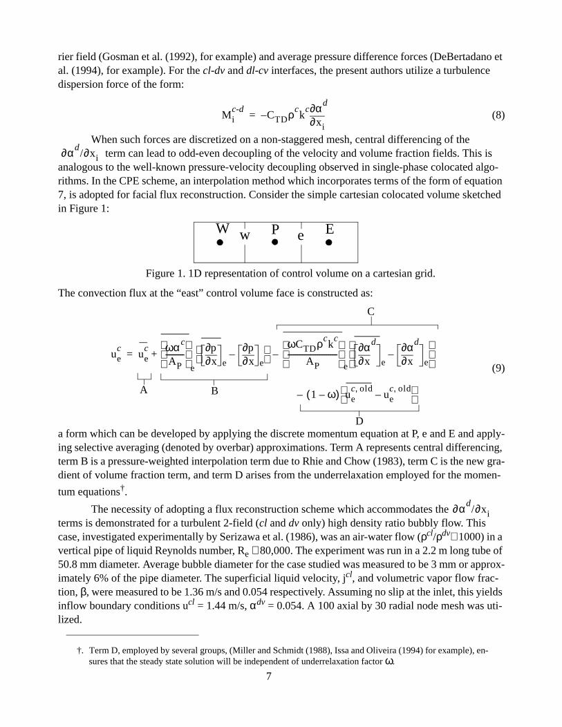
analogous to the well-known pressure-velocity decoupling observed in single-phase colocated algo-rithms. In the CPE scheme, an interpolation method which incorporates terms of the form of equation 7, is adopted for facial flux reconstruction. Consider the simple cartesian colocated volume sketched in Figure 1:

The convection flux at the “east” control volume face is constructed as:

(9)

a form which can be developed by applying the discrete momentum equation at P, e and E and apply-ing selective averaging (denoted by overbar) approximations. Term A represents central differencing, term B is a pressure-weighted interpolation term due to Rhie and Chow (1983), term C is the new gra-dient of volume fraction term, and term D arises from the underrelaxation employed for the momen-

tum equations†.

The necessity of adopting a flux reconstruction scheme which accommodates the terms is demonstrated for a turbulent 2-field (cl and dv only) high density ratio bubbly flow. This case, investigated experimentally by Serizawa et al. (1986), was an air-water flow (ρcl/ρdv≅ 1000) in a vertical pipe of liquid Reynolds number, Re ≅ 80,000. The experiment was run in a 2.2 m long tube of 50.8 mm diameter. Average bubble diameter for the case studied was measured to be 3 mm or approx-imately 6% of the pipe diameter. The superficial liquid velocity, jcl, and volumetric vapor flow frac-tion, β, were measured to be 1.36 m/s and 0.054 respectively. Assuming no slip at the inlet, this yields inflow boundary conditions ucl = 1.44 m/s, αdv = 0.054. A 100 axial by 30 radial node mesh was uti-lized.

†. Term D, employed by several groups, (Miller and Schmidt (1988), Issa and Oliveira (1994) for example), en-sures that the steady state solution will be independent of underrelaxation factor ω.

Mic-d

CTDρck

c

xi∂∂αd

–=

∂αd/∂xi

Figure 1. 1D representation of control volume on a cartesian grid.

P EW ew

uec

uec ωαc

AP----------

ex∂

∂pe x∂

∂pe

–

ωCTDρck

c

AP---------------------------

e x∂∂αd

e x∂∂αd

e–

–+=

1 ω–( ) uec old,

uec old,

– –

C

BA

D

∂αd/∂xi

7

Two runs were made, one with term C included in equation 9, one without. Figure 2a shows a comparison of predicted and measured outlet velocity profiles. The analyses accurately predict the flattening of the liquid velocity profile, compared to a single phase calculation run using the same superficial liquid velocity. When term C is not included in the discretization, the predicted velocity profile underpredicts this flattening. Figure 2b shows a comparison between predicted and measured outlet vapor volume fraction profiles. Agreement here is excellent for the improved discretization. However, it can be seen that neglect of the turbulence dispersion term in the flux reconstruction leads to highly oscillatory volume fraction predictions. Both simulations converged to machine accuracy, as shown in Figure 2c, though the improved discretization allowed for larger underrelaxation factors to be used for the momentum and volume fraction equations, giving rise to the significantly improved convergence rates shown.

It has been demonstrated that the inclusion of dispersive interfacial force terms is critical in the facial flux reconstruction procedure. In general, any force appearing in the momentum equations, which varies non-linearly in space, can be introduced. In single phase applications, Gu (1991) and others have found it necessary to include buoyancy terms in the flux evaluation for thermally driven flows. The present authors have found that including gravity and other force terms (including lift) can

0.0 0.2 0.4 0.6 0.8 1.00.8

1.0

1.2

1.4

1.6

1.8

r/R

U(m/s)

Data

Term C included

Term C not included

Single phase result

0 250 500 750 1000

-10

-5

0

log10ERROR

Iteration

Term C Included

Term C Not Included

0.0 0.2 0.4 0.6 0.8 1.00.00

0.05

0.10

0.15

0.20

0.25

r/R

αdv

Data

Term C included

Term C not included

Figure 2. Serizawa’s (1986) turbulent bubbly flow in a vertical pipe. a) Comparison of outlet cl velocity distributions. b) Comparison of outlet dv volume fraction distributions. c) Comparison

of convergence characteristics for two flux evaluation schemes.

a) b)

c)

8

be somewhat beneficial to solution convergence and accuracy, but in general is not as critical as

including terms.

2) Phase Coupled Linear Solution of Scalar Transport Variables

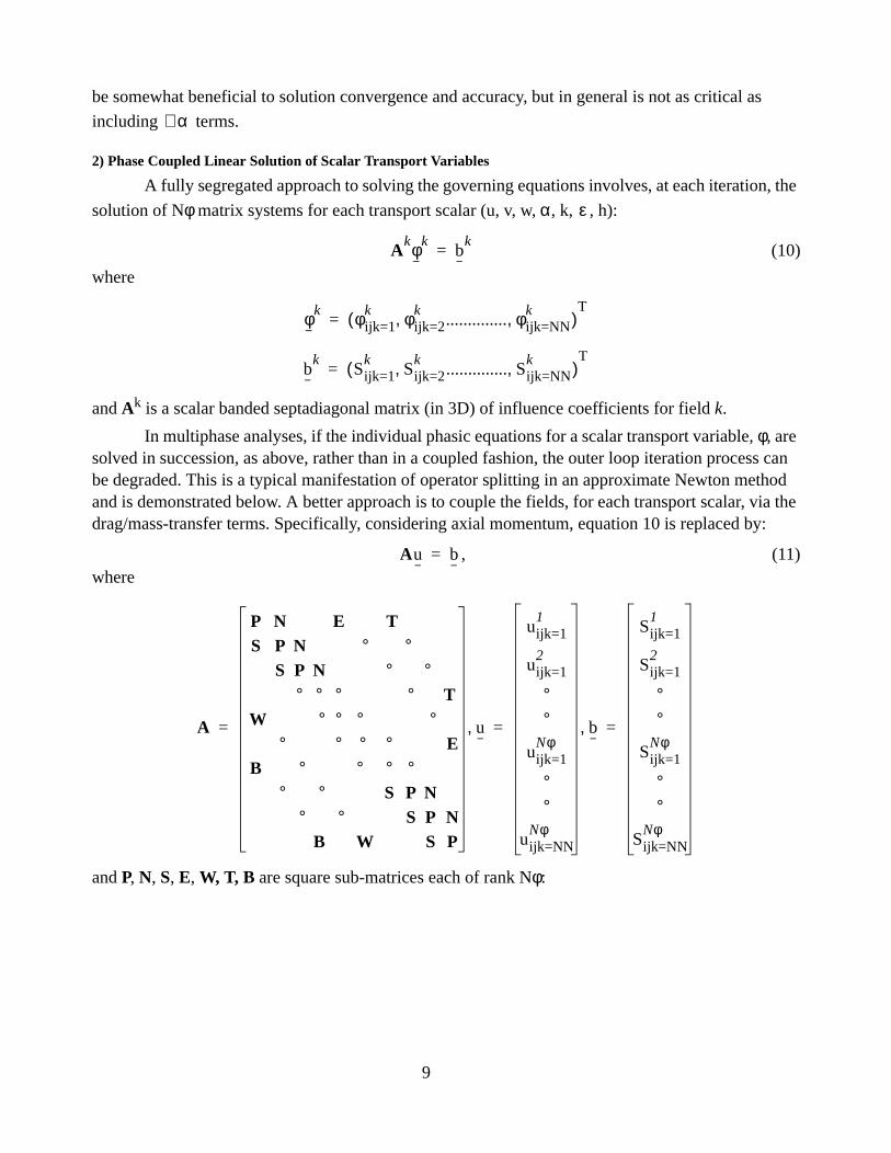
A fully segregated approach to solving the governing equations involves, at each iteration, the

solution of Nφ matrix systems for each transport scalar (u, v, w, α, k, , h):

(10)

where

and Ak is a scalar banded septadiagonal matrix (in 3D) of influence coefficients for field k.

In multiphase analyses, if the individual phasic equations for a scalar transport variable, φ, are solved in succession, as above, rather than in a coupled fashion, the outer loop iteration process can be degraded. This is a typical manifestation of operator splitting in an approximate Newton method and is demonstrated below. A better approach is to couple the fields, for each transport scalar, via the drag/mass-transfer terms. Specifically, considering axial momentum, equation 10 is replaced by:

, (11)where

and P, N, S, E, W, T, B are square sub-matrices each of rank Nφ:

∇α

ε

Akφk

bk

=

φk φijk=1k φijk=2

k.............. φijk=NN

k, ,( )T

=

bk

Sijk=1k

Sijk=2k

.............. Sijk=NNk, ,( )

T=

Au b=

A

P N E T S P N ° ° S P N ° ° ° ° ° ° T

W ° ° ° °

° ° ° ° EB ° ° ° ° ° ° S P N

° ° S P N B W S P

u,

uijk=11

uijk=12

°°

uijk=1Nφ

°°

uijk=NNNφ

b,

Sijk=11

Sijk=12

°°

Sijk=1Nφ

°°

Sijk=NNNφ

= = =

9

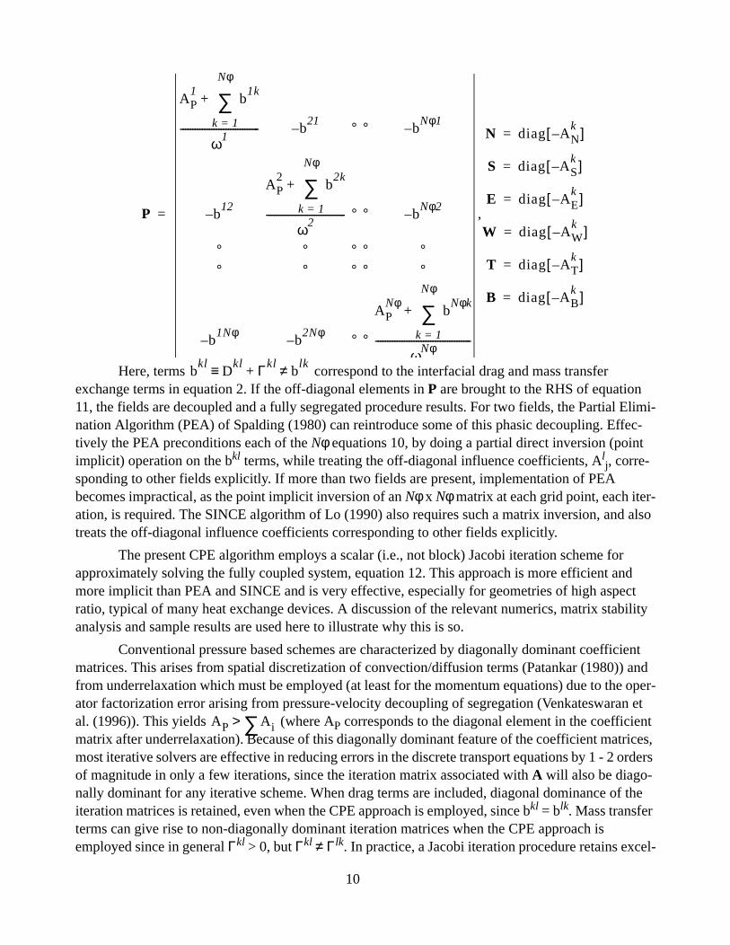
Here, terms correspond to the interfacial drag and mass transfer exchange terms in equation 2. If the off-diagonal elements in P are brought to the RHS of equation 11, the fields are decoupled and a fully segregated procedure results. For two fields, the Partial Elimi-nation Algorithm (PEA) of Spalding (1980) can reintroduce some of this phasic decoupling. Effec-tively the PEA preconditions each of the Nφ equations 10, by doing a partial direct inversion (point implicit) operation on the bkl terms, while treating the off-diagonal influence coefficients, Al

j, corre-sponding to other fields explicitly. If more than two fields are present, implementation of PEA becomes impractical, as the point implicit inversion of an Nφ x Nφ matrix at each grid point, each iter-ation, is required. The SINCE algorithm of Lo (1990) also requires such a matrix inversion, and also treats the off-diagonal influence coefficients corresponding to other fields explicitly.

The present CPE algorithm employs a scalar (i.e., not block) Jacobi iteration scheme for approximately solving the fully coupled system, equation 12. This approach is more efficient and more implicit than PEA and SINCE and is very effective, especially for geometries of high aspect ratio, typical of many heat exchange devices. A discussion of the relevant numerics, matrix stability analysis and sample results are used here to illustrate why this is so.

Conventional pressure based schemes are characterized by diagonally dominant coefficient matrices. This arises from spatial discretization of convection/diffusion terms (Patankar (1980)) and from underrelaxation which must be employed (at least for the momentum equations) due to the oper-ator factorization error arising from pressure-velocity decoupling of segregation (Venkateswaran et al. (1996)). This yields (where AP corresponds to the diagonal element in the coefficient matrix after underrelaxation). Because of this diagonally dominant feature of the coefficient matrices, most iterative solvers are effective in reducing errors in the discrete transport equations by 1 - 2 orders of magnitude in only a few iterations, since the iteration matrix associated with A will also be diago-nally dominant for any iterative scheme. When drag terms are included, diagonal dominance of the iteration matrices is retained, even when the CPE approach is employed, since bkl = blk. Mass transfer terms can give rise to non-diagonally dominant iteration matrices when the CPE approach is employed since in general Γkl > 0, but Γkl ≠ Γlk. In practice, a Jacobi iteration procedure retains excel-

P

AP1

b1k

k 1=

Nφ

∑+

ω1--------------------------------- b–

21 ° ° bNφ1

–

b12

–

AP2

b2k

k 1=

Nφ

∑+

ω2--------------------------------- ° ° b

Nφ2–

° ° ° ° °° ° ° ° °

b1Nφ

– b2Nφ

– ° °

APNφ

bNφk

k 1=

Nφ

∑+

ωNφ----------------------------------------

,

N diag A– Nk[ ]=

S diag A– Sk[ ]=

E diag A– Ek[ ]=

W diag A– Wk[ ]=

T diag A– Tk[ ]=

B diag A– Bk[ ]=

=

bkl

Dkl Γkl

blk≠+≡

AP Ai∑>

10

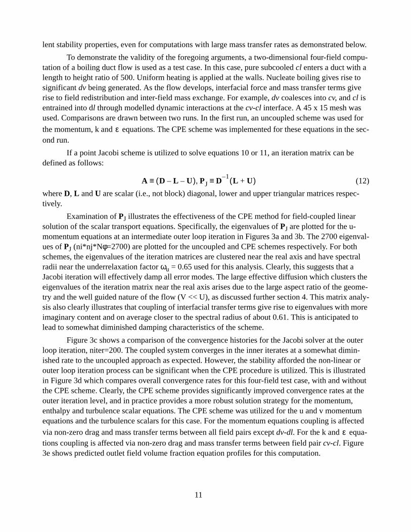
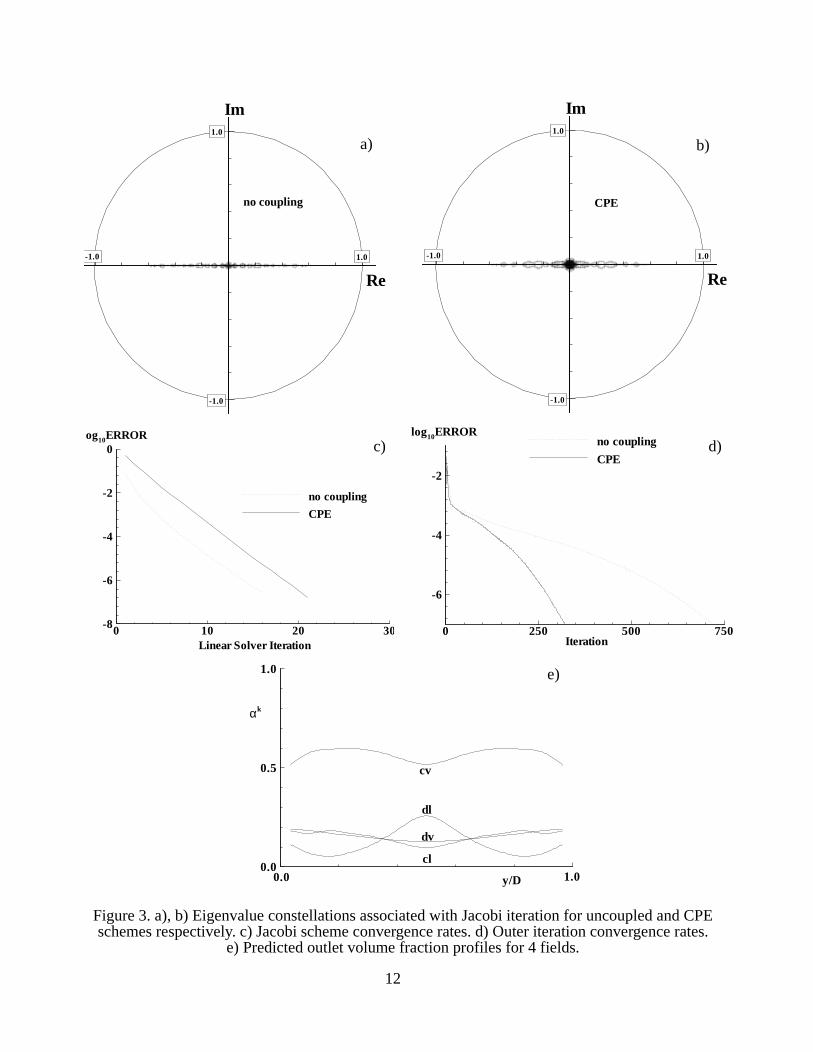
lent stability properties, even for computations with large mass transfer rates as demonstrated below.

To demonstrate the validity of the foregoing arguments, a two-dimensional four-field compu-tation of a boiling duct flow is used as a test case. In this case, pure subcooled cl enters a duct with a length to height ratio of 500. Uniform heating is applied at the walls. Nucleate boiling gives rise to significant dv being generated. As the flow develops, interfacial force and mass transfer terms give rise to field redistribution and inter-field mass exchange. For example, dv coalesces into cv, and cl is entrained into dl through modelled dynamic interactions at the cv-cl interface. A 45 x 15 mesh was used. Comparisons are drawn between two runs. In the first run, an uncoupled scheme was used for

the momentum, k and equations. The CPE scheme was implemented for these equations in the sec-ond run.

If a point Jacobi scheme is utilized to solve equations 10 or 11, an iteration matrix can be defined as follows:

(12)

where D, L and U are scalar (i.e., not block) diagonal, lower and upper triangular matrices respec-tively.

Examination of PJ illustrates the effectiveness of the CPE method for field-coupled linear solution of the scalar transport equations. Specifically, the eigenvalues of PJ are plotted for the u-momentum equations at an intermediate outer loop iteration in Figures 3a and 3b. The 2700 eigenval-ues of PJ (ni*nj*Nφ=2700) are plotted for the uncoupled and CPE schemes respectively. For both schemes, the eigenvalues of the iteration matrices are clustered near the real axis and have spectral radii near the underrelaxation factor ωu = 0.65 used for this analysis. Clearly, this suggests that a Jacobi iteration will effectively damp all error modes. The large effective diffusion which clusters the eigenvalues of the iteration matrix near the real axis arises due to the large aspect ratio of the geome-try and the well guided nature of the flow (V << U), as discussed further section 4. This matrix analy-sis also clearly illustrates that coupling of interfacial transfer terms give rise to eigenvalues with more imaginary content and on average closer to the spectral radius of about 0.61. This is anticipated to lead to somewhat diminished damping characteristics of the scheme.

Figure 3c shows a comparison of the convergence histories for the Jacobi solver at the outer loop iteration, niter=200. The coupled system converges in the inner iterates at a somewhat dimin-ished rate to the uncoupled approach as expected. However, the stability afforded the non-linear or outer loop iteration process can be significant when the CPE procedure is utilized. This is illustrated in Figure 3d which compares overall convergence rates for this four-field test case, with and without the CPE scheme. Clearly, the CPE scheme provides significantly improved convergence rates at the outer iteration level, and in practice provides a more robust solution strategy for the momentum, enthalpy and turbulence scalar equations. The CPE scheme was utilized for the u and v momentum equations and the turbulence scalars for this case. For the momentum equations coupling is affected

via non-zero drag and mass transfer terms between all field pairs except dv-dl. For the k and equa-tions coupling is affected via non-zero drag and mass transfer terms between field pair cv-cl. Figure 3e shows predicted outlet field volume fraction equation profiles for this computation.

ε

A D L– U–( ) PJ D1–

L U+( )≡,≡

ε

11

Im

Re

1.0

1.0

-1.0

-1.0

Im

Re

1.0

1.0

-1.0

-1.0

0 10 20 30-8

-6

-4

-2

0og10ERROR

Linear Solver Iteration

no coupling

CPE

0 250 500 750

-6

-4

-2

log10ERROR

Iteration

no coupling

CPE

0.0

0.5

1.0

cl

dv

cv

dl

y/D 1.00.0

αk

Figure 3. a), b) Eigenvalue constellations associated with Jacobi iteration for uncoupled and CPE schemes respectively. c) Jacobi scheme convergence rates. d) Outer iteration convergence rates.

e) Predicted outlet volume fraction profiles for 4 fields.

no coupling CPE

a) b)

c) d)

e)

12

Because of linearization errors and factorization errors associated with variable segregation, it is typically only useful to reduce the linear solver errors by approximately 1-2 orders of magnitude for each transport scalar, at each outer loop iteration. Figure 3c shows that this is achievable is only a few Jacobi sweeps. The Jacobi solver in the present scheme combines both a low operation count per sweep compared to more complex iterative solvers, and executes in excess of 550 MFLOPS on a Cray C90. Since linear solution of scalar matrix systems accounts for a significant contribution of the overall CPU burden in four field solutions, this performance contributes to a very efficient scheme. The CPE scheme retains the same very high vector CPU performance as the uncoupled scheme due to vectorizability and low operation count.

3) Interfacial Transfer Consistent Pressure-Velocity Correction Scheme.

Two methods can be employed in the CPE algorithm to satisfy mass conservation. In the stan-dard method, adopted for clarity of presentation in this section (section 6 below introduces an improved scheme), a mixture volume conservation equation is derived by summing individual field volume fraction equations, each normalized by field density. A pressure-velocity corrector relation is applied to develop an elliptic pressure correction equation. Transport equations for the field volume fraction equations are then solved. This standard method has been adopted by several workers includ-ing Spalding (1980), Carver and Salcudean (1986) and Issa and Oliveira (1994).

In the CPE algorithm, a generalized pressure-velocity coupling is developed based on the field coupled momentum equations. Consider the field coupled momentum equations 11, written as:

(13)Adopting a corrector formulation, equation 13 leads to the pressure-velocity coupling relationship:

(14)

where

Following conventional single-phase pressure-correction algorithm development, A is approximated by neglecting all spatial coupling terms:

, (15)Where P is defined with equation 11. This form retains full field coupling of the drag and mass trans-fer terms. At each node, the pressure-velocity coupling relation becomes

, (16)

where now

and

u A1–b=

u’ A1–b

p=

bp

α1V

p’∂x∂

-------–

ijk=1α2

Vp'∂x∂

-------–

ijk=1.. αNφ

Vp'∂x∂

-------–

ijk=1.... αNφ

Vp'∂x∂

-------–

ijk=NN, , , , ,

T=

A A diag P( )≡∼

u’ P* 1–

bp

=

u’ u’1

u’2

.. u’Nφ, , ,( )

T= b

pα1

Vp’∂x∂

-------– α2V

p'∂x∂

-------– .. αNφV

p'∂x∂

-------–, , , T

=, Vp'∂x∂

------- α1– α2

– .. αNφ–, , ,( )

T=

P*

P diag ωkAj

k

j=NSEWTB∑

–≡

13

14

Replacing P with P* corresponds to adopting the SIMPLEC over SIMPLE approximation in neglect-ing spatial coupling.

For field k, equation 16 leads to the velocity correction equation:

(17)

Equation 17 is used to derive the mixture volume pressure correction equation. Specifically, the velocity decomposition:

(18)

is adopted, where corresponds to velocity components available after solution of the momentum equations. Equation 18 is substituted into each of the field continuity equations, which are then nor-

malized by their density and summed. Substituting equation 17 for , and applying second order central differencing for the gradient of the pressure corrector, the resulting equation can be written in cartesian coordinates as:

(19)

Here, subscript [--]ew denotes the difference [--]e- [--]w (see figure 1), ∆p’ corresponds to the

difference across the face (i.e., ∆p’e = p’E - p’W), and represents the local imbalance in field mass arising from the velocities computed in the momentum equations. Equation 19 can be cast in a form similar to equation 6:

(20)

When a colocated variable arrangement is employed, an approximate pressure-velocity cou-pling is also typically introduced in the inviscid flux reconstruction at cell faces (i.e., Rhie-Chow interpolation). Developments analogous to those presented above are used to derive a consistent facial flux reconstruction strategy in the CPE algorithm, yielding:

(21)

Equations 17 and 21, represent the best possible phasic pressure-velocity coupling achievable for the frozen coefficient linearization adopted.

The evaluation of in equation 17, requires the inversion of several 4 x 4 matrices at each grid point, at each iteration. This potentially CPU intensive procedure is circumvented by applying a simple Jacobi fixed point iterative procedure to approximately invert P and P*. This procedure is vec-torizable and rapidly convergent (2 sweeps are employed) for the same reason that the Jacobi proce-

u'k

Dk

V–p'∂x∂

------- = D

k, αlP

* 1–( )

kl

l=1,Nφ∑

≡

uk

u*k

u'k

+≡

u*k

u'k

αkD

k

k=1,Nφ∑

∆y∆z( )2∆p'

ns

– αkD

k

k=1,Nφ∑

∆x∆z( )2∆p'

ew

– –

αkD

k

φ∑

∆x∆y( )2∆p'm·

*k

ρk---------

φ∑–=

m·*k

APp'P Ajp'jj=NSEWTB

∑ m·*k

ρk---------

k=1,Nφ∑–=

uek

uek

Bek

x∂∂p

e x∂∂p

e–

Aek

x∂∂αd

e x∂∂αd

e–

, –+=

Bk α l

P1–( )

kl

l=1,Nφ∑= A

kCTDρc

kc

P1–( )

kl

l=1,Nφ∑=,

Dk

dure is an effective linear equation solver for the scalar transport equations in these flows. Specifically, the P matrices are very well conditioned, due to the presence of underrelaxation and the clustering of its eigenvalues near the real axis.

In Figure 4, the impact of the improved pressure-velocity coupling on outer loop convergence is demonstrated for the same four-field boiling duct flow problem used for testing in the previous sec-tion. For this 2D problem, four cases were run. In the first case, all off-diagonal terms in matrix P are zeroed in equations 17 and 21. This corresponds to neglecting all phasic coupling in the flux recon-struction and pressure correction coefficient assembly steps. In case 2, only those off-diagonal terms in matrix P corresponding to cl-dv and dl-cv exchange were included (condensation/evaporation at bubble and droplet interfaces, bubble and droplet drag). In case 3, cl-cv exchange were added (film boiling/evaporation, film drag). In case 4 the remaining inter-field exchange terms, cl-dl, cv-dv, were included (bubble coalescence and breakup, droplet entrainment and deposition). The figure shows that converged solutions were obtained all cases. However the maximum obtainable convergence rate, obtained when the complete phasic pressure-velocity coupling was employed, was significantly greater than for cases 1 through 3.

4) Additive Correction Strategy for Pressure Poisson Equation

In section 2 it was demonstrated that a field-coupled Jacobi iteration procedure is effective for solving the scalar transport systems which arise in the four-field formulation. Additional consider-ations arise, when solving the pressure Poisson equation, which must be addressed in constructing an efficient overall scheme. Specifically, significant stiffness can arise when iterative schemes are applied to solve the pressure corrector equation on geometries of even moderate aspect ratio.

One can usefully analyze the convergence characteristics of iterative schemes applied to the mixture continuity equation by considering the model problem:

(22)

where equation 22 can be obtained from equation 20 by taking that influence coefficients, Aj, AP, do

0 250 500

-6

-4

-2

log10ERROR

Iteration

no coupling

cl-dv,dl-cv

cl-dv,dl-cv,cl-cv

cl-dv,dl-cv,cl-cv,cl-dl,cv-dv

Figure 4. Comparison of pressure-velocity coupling treatments.

ν1δxxp’ ν2δyyp’ ν3δzzp’+ + S=

15

16

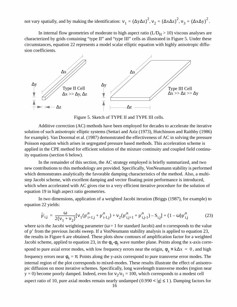
not vary spatially, and by making the identification: .

In internal flow geometries of moderate to high aspect ratio (L/DH > 10) viscous analyses are characterized by grids containing “type II” and “type III” cells as illustrated in Figure 5. Under these circumstances, equation 22 represents a model scalar elliptic equation with highly anisotropic diffu-sion coefficients.

Additive correction (AC) methods have been employed for decades to accelerate the iterative solution of such anisotropic elliptic systems (Settari and Aziz (1973), Hutchinson and Raithby (1986) for example). Van Doormal et al. (1987) demonstrated the effectiveness of AC in solving the pressure Poisson equation which arises in segregated pressure based methods. This acceleration scheme is applied in the CPE method for efficient solution of the mixture continuity and coupled field continu-ity equations (section 6 below).

In the remainder of this section, the AC strategy employed is briefly summarized, and two new contributions to this methodology are provided. Specifically, VonNeumann stability is performed which demonstrates analytically the favorable damping characteristics of the method. Also, a multi-step Jacobi scheme, with excellent damping and vector floating point performance is introduced, which when accelerated with AC gives rise to a very efficient iterative procedure for the solution of equation 19 in high aspect ratio geometries.

In two dimensions, application of a weighted Jacobi iteration (Briggs (1987), for example) to equation 22 yields:

(23)

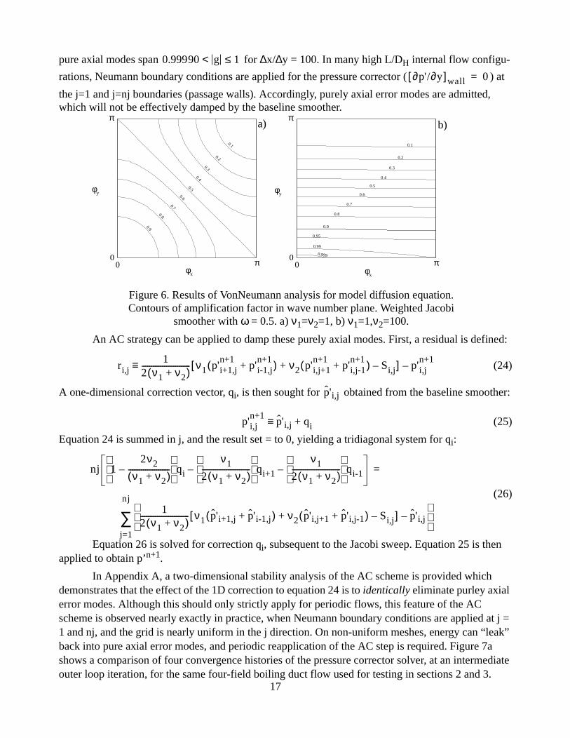
where ω is the Jacobi weighting parameter (ω = 1 for standard Jacobi) and n corresponds to the value of p’ from the previous Jacobi sweep. If a VonNeumann stability analysis is applied to equation 23, the results in Figure 6 are obtained. These plots show contours of amplification factor for a weighted Jacobi scheme, applied to equation 23, in the φx-φy wave number plane. Points along the x-axis corre-

spond to pure axial error modes, with low frequency errors near the origin, , and high

frequency errors near φx = π. Points along the y-axis correspond to pure transverse error modes. The internal region of the plot corresponds to mixed-modes. These results illustrate the effect of anisotro-pic diffusion on most iterative schemes. Specifically, long wavelength transverse modes (region near y = 0) become poorly damped. Indeed, even for ν2/ν1 = 100, which corresponds to a modest cell

aspect ratio of 10, pure axial modes remain nearly undamped ( ). Damping factors for

ν1 ∆y∆z( )2= ν2 ∆x∆z( )2

= ν3 ∆x∆y( )2=, ,

Type II Cell∆x >> ∆y, ∆z

Type III Cell∆x >> ∆z >> ∆y

∆z

∆y

∆x ∆x

∆y

∆z

Figure 5. Sketch of TYPE II and TYPE III cells.

p'ˆ i,jω

2 ν1 ν2+( )-------------------------- ν1 p'i+1,j

np'i-1,j

n+( ) ν2 p'i,j+1

np'i,j-1

n+( ) Si,j–+[ ] 1 ω–( )p'i,j

n+=

φx k∆x≡ 0=

0.990 g 1≤<

17

pure axial modes span for ∆x/∆y = 100. In many high L/DH internal flow configu-

rations, Neumann boundary conditions are applied for the pressure corrector ( ) at

the j=1 and j=nj boundaries (passage walls). Accordingly, purely axial error modes are admitted, which will not be effectively damped by the baseline smoother.

An AC strategy can be applied to damp these purely axial modes. First, a residual is defined:

(24)

A one-dimensional correction vector, qi, is then sought for obtained from the baseline smoother:

(25)

Equation 24 is summed in j, and the result set = to 0, yielding a tridiagonal system for qi:

(26)

Equation 26 is solved for correction qi, subsequent to the Jacobi sweep. Equation 25 is then applied to obtain p’n+1.

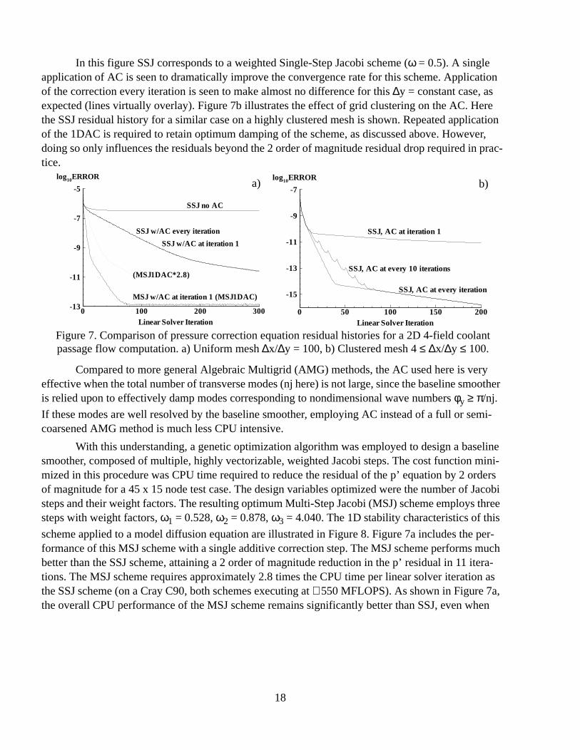
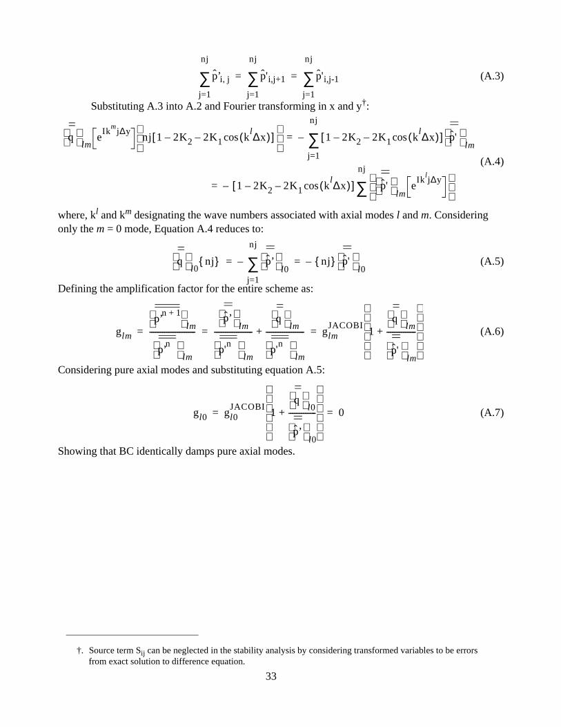
In Appendix A, a two-dimensional stability analysis of the AC scheme is provided which demonstrates that the effect of the 1D correction to equation 24 is to identically eliminate purley axial error modes. Although this should only strictly apply for periodic flows, this feature of the AC scheme is observed nearly exactly in practice, when Neumann boundary conditions are applied at j = 1 and nj, and the grid is nearly uniform in the j direction. On non-uniform meshes, energy can “leak” back into pure axial error modes, and periodic reapplication of the AC step is required. Figure 7a shows a comparison of four convergence histories of the pressure corrector solver, at an intermediate outer loop iteration, for the same four-field boiling duct flow used for testing in sections 2 and 3.

0.99990 g 1≤<∂p'/∂y[ ] wall 0=

0.1

0.2

0.4

0.6

0.7

0.8

0.9

0.3

0.5

π

π00

φx

φy

Figure 6. Results of VonNeumann analysis for model diffusion equation. Contours of amplification factor in wave number plane. Weighted Jacobi

smoother with ω = 0.5. a) ν1=ν2=1, b) ν1=1,ν2=100.

0.1

0.95

0.99

0.999

0.2

0.3

0.4

0.5

0.6

0.7

0.8

0.9

π

π00

φx

φy

a) b)

ri,j1

2 ν1 ν2+( )-------------------------- ν1 p'i+1,j

n+1p'i-1,j

n+1+( ) ν2 p'i,j+1

n+1p'i,j-1

n+1+( ) Si,j–+[ ] p'i,j

n+1–≡

p'ˆ i,j

p'i,jn+1

p'ˆ i,j qi+≡

nj 12ν2

ν1 ν2+( )----------------------–

qi

ν1

2 ν1 ν2+( )--------------------------

qi+1–ν1

2 ν1 ν2+( )--------------------------

qi-1– =

12 ν1 ν2+( )-------------------------- ν1 p'ˆ i+1,j p'ˆ i-1,j+( ) ν2 p'ˆ i,j+1 p'ˆ i,j-1+( ) Si,j–+[ ] p'ˆ i,j–

j=1

nj

∑

In this figure SSJ corresponds to a weighted Single-Step Jacobi scheme (ω = 0.5). A single application of AC is seen to dramatically improve the convergence rate for this scheme. Application of the correction every iteration is seen to make almost no difference for this ∆y = constant case, as expected (lines virtually overlay). Figure 7b illustrates the effect of grid clustering on the AC. Here the SSJ residual history for a similar case on a highly clustered mesh is shown. Repeated application of the 1DAC is required to retain optimum damping of the scheme, as discussed above. However, doing so only influences the residuals beyond the 2 order of magnitude residual drop required in prac-tice.

Compared to more general Algebraic Multigrid (AMG) methods, the AC used here is very effective when the total number of transverse modes (nj here) is not large, since the baseline smoother is relied upon to effectively damp modes corresponding to nondimensional wave numbers φy ≥ π/nj.

If these modes are well resolved by the baseline smoother, employing AC instead of a full or semi-coarsened AMG method is much less CPU intensive.

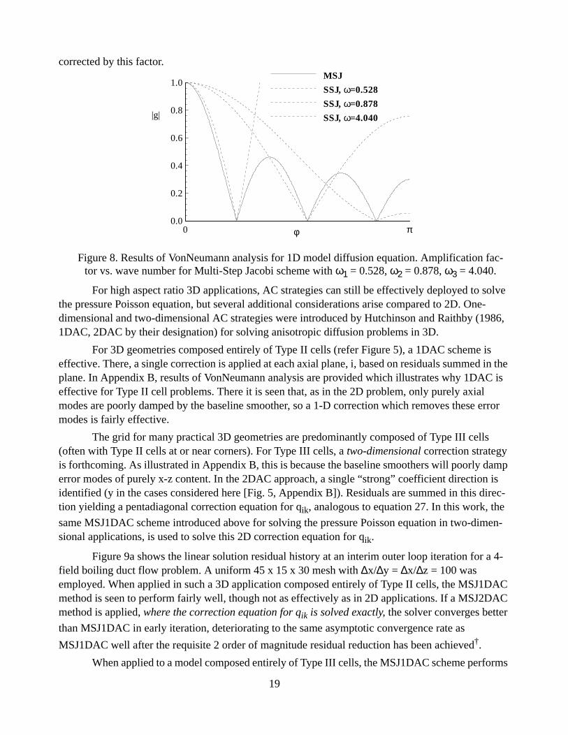
With this understanding, a genetic optimization algorithm was employed to design a baseline smoother, composed of multiple, highly vectorizable, weighted Jacobi steps. The cost function mini-mized in this procedure was CPU time required to reduce the residual of the p’ equation by 2 orders of magnitude for a 45 x 15 node test case. The design variables optimized were the number of Jacobi steps and their weight factors. The resulting optimum Multi-Step Jacobi (MSJ) scheme employs three steps with weight factors, ω1 = 0.528, ω2 = 0.878, ω3 = 4.040. The 1D stability characteristics of this

scheme applied to a model diffusion equation are illustrated in Figure 8. Figure 7a includes the per-formance of this MSJ scheme with a single additive correction step. The MSJ scheme performs much better than the SSJ scheme, attaining a 2 order of magnitude reduction in the p’ residual in 11 itera-tions. The MSJ scheme requires approximately 2.8 times the CPU time per linear solver iteration as the SSJ scheme (on a Cray C90, both schemes executing at ≅ 550 MFLOPS). As shown in Figure 7a, the overall CPU performance of the MSJ scheme remains significantly better than SSJ, even when

0 100 200 300-13

-11

-9

-7

-5

log10ERROR

Linear Solver Iteration

MSJ w/AC at iteration 1 (MSJ1DAC)

SSJ w/AC at iteration 1

SSJ w/AC every iteration

SSJ no AC

(MSJ1DAC*2.8)

0 50 100 150 200

-15

-13

-11

-9

-7

log10ERROR

Linear Solver Iteration

SSJ, AC at every 10 iterations

SSJ, AC at iteration 1

SSJ, AC at every iteration

Figure 7. Comparison of pressure correction equation residual histories for a 2D 4-field coolant passage flow computation. a) Uniform mesh ∆x/∆y = 100, b) Clustered mesh 4 ≤ ∆x/∆y ≤ 100.

a) b)

18

corrected by this factor.

For high aspect ratio 3D applications, AC strategies can still be effectively deployed to solve the pressure Poisson equation, but several additional considerations arise compared to 2D. One-dimensional and two-dimensional AC strategies were introduced by Hutchinson and Raithby (1986, 1DAC, 2DAC by their designation) for solving anisotropic diffusion problems in 3D.

For 3D geometries composed entirely of Type II cells (refer Figure 5), a 1DAC scheme is effective. There, a single correction is applied at each axial plane, i, based on residuals summed in the plane. In Appendix B, results of VonNeumann analysis are provided which illustrates why 1DAC is effective for Type II cell problems. There it is seen that, as in the 2D problem, only purely axial modes are poorly damped by the baseline smoother, so a 1-D correction which removes these error modes is fairly effective.

The grid for many practical 3D geometries are predominantly composed of Type III cells (often with Type II cells at or near corners). For Type III cells, a two-dimensional correction strategy is forthcoming. As illustrated in Appendix B, this is because the baseline smoothers will poorly damp error modes of purely x-z content. In the 2DAC approach, a single “strong” coefficient direction is identified (y in the cases considered here [Fig. 5, Appendix B]). Residuals are summed in this direc-tion yielding a pentadiagonal correction equation for qik, analogous to equation 27. In this work, the

same MSJ1DAC scheme introduced above for solving the pressure Poisson equation in two-dimen-sional applications, is used to solve this 2D correction equation for qik.

Figure 9a shows the linear solution residual history at an interim outer loop iteration for a 4-field boiling duct flow problem. A uniform 45 x 15 x 30 mesh with ∆x/∆y = ∆x/∆z = 100 was employed. When applied in such a 3D application composed entirely of Type II cells, the MSJ1DAC method is seen to perform fairly well, though not as effectively as in 2D applications. If a MSJ2DAC method is applied, where the correction equation for qik is solved exactly, the solver converges better

than MSJ1DAC in early iteration, deteriorating to the same asymptotic convergence rate as

MSJ1DAC well after the requisite 2 order of magnitude residual reduction has been achieved†.

When applied to a model composed entirely of Type III cells, the MSJ1DAC scheme performs

0.0

0.2

0.4

0.6

0.8

1.0

φ0 π

|g|

MSJ

SSJ, ω=0.528

SSJ, ω=0.878

SSJ, ω=4.040

Figure 8. Results of VonNeumann analysis for 1D model diffusion equation. Amplification fac-tor vs. wave number for Multi-Step Jacobi scheme with ω1 = 0.528, ω2 = 0.878, ω3 = 4.040.

19

poorly, because mixed modes characterized by 0 ≤ φx ≤ π, φy = 0, π/nk ≤ φz ≤ π are not well damped

(Appendix B). This is illustrated in Figure 9b, which is analogous to 9a, except that a uniform 45 x 15 x 30 mesh with ∆x/∆y = 100, ∆x/∆z = 10 was utilized. For such meshes, the MSJ2DAC scheme is seen to be very effective. Indeed, a 2-3 order of magnitude drop in the p’ residual is observed in approximately 10 sweeps. In design applications, Type II and Type III cells coexist due to grid clus-tering. In these mixed cell-type problems, results presented for the Type III cells in Figure 9b, closely represent the performance of the MSJ1DAC and MSJ2DAC schemes.

It is not necessary or computationally efficient to exactly solve the 2D correction equation for qik which arises in the 2DAC scheme. If the qik correction equation is solved approximately, conver-gence for the p’ equation will deteriorate. In practice, this system is solved to a two order of magni-tude residual reduction, which in turn ensures that this deterioration does not manifest itself until after the required 2 order of magnitude drop in the p’ equation residual. This is illustrated in Figure 9b, where scheme MSJ2DAC* represents an approximate solution of the qik system.

In the authors’ code, MSJ1DAC is employed for 2D problems: 10 sweeps of the MSJ scheme are applied with a single 1DAC step. A single 1DAC step is acceptable even on clustered meshes. For 3D problems, which contain Type II and III cells, MSJ2DAC is employed: 10 sweeps of the MSJ smoother are applied with 2DAC steps applied every 5 MSJ sweeps. Adequate convergence of the qik equation in the 2DAC step is achieved by applying 30 MSJ sweeps, with 1DAC steps applied every 5 MSJ sweeps. The convergence history labelled MSJ2DAC* in Figure 9b, corresponds to application of this strategy there.

Though the AC method described above is very effective for the high aspect ratio geometries and grids of principal relevance to the authors, its performance deteriorates as cell aspect ratios approach unity and as the number of transverse nodes increases. In these circumstances, more general multigrid approaches, i.e. full or semi-coarsening AMG methods, represent the generalization of the methodology described, and should be deployed.

†. This asymptotic rate corresponding to the largest eigenvalue in the system undamped by either 1DAC or 2DAC steps: 0 ≤ φx ≤ π, φy = π/nj, φz = 0, (see Figure A1).

0 20 40 60 80 100-13

-11

-9

-7

-5

log10ERROR

Linear Solver Iteration

MSJ1DAC

MSJ2DAC

0 20 40 60 80 100-13

-11

-9

-7

-5

-3

log10ERROR

Linear Solver Iteration

MSJ1DAC

MSJ2DAC

MSJ2DAC*

Figure 9. Comparison of the performance of MSJ1DAC and MSJ2DAC schemes for 3D problems composed entirely of a) Type II cells, b) Type III cells.

a) b)

20

5) Realizability Enforcing Implicit Source Treatment for Volume Fraction Equations

Satisfactory mass transfer and interfacial force models which appear must satisfy many physi-cal requirements (Drew (1992)). Among these, clearly, is the realizability of the field volume frac-tions, 0 ≤ α ≤ 1. Both mass transfer and interfacial force models can be formulated which violate realizability differentially or discretely. The authors and their co-workers have formulated a model set which returns converged solutions which do not violate volume fraction realizability (with the excep-tion of several pathological cases). However, during the course of iteration, special case must be taken to ensure that volume fractions remain realizable, or else the iterative procedure can be non-conver-gent.

An analogous situation arises in turbulence modelling, where turbulence scalars (k and for example) must remain realizable. A simple lagged approach proposed by Huang and Leschziner (1985) for treating Reynolds stress model source terms can ensure the positivity of positive quantities. In particular, consider the discrete transport equation for positive scalar φ:

(27)

where Φ+ and Φ- are positive and negative source terms respectively. The simple lagged coefficient linearization:

(28)

ensures that φn+1 ≥ 0, for φn ≥ 0†.

A straightforward extension of this procedure is used in the CPE method to ensure volume

fraction realizability. Consider the discrete transport equation for field volume fraction αk:

(29)

where and are positive and negative net mass transfer rates respec-

tively. Realizability is assured by adopting the lagged coefficient linearization:

(30)

6) Field Continuity Coupling via Pressure-Volume Fraction-Velocity Correction Scheme

As summarized in Section 3, continuity can be satisfied by solving a mixture volume pres-sure-correction equation, and then solving transport equations for the field volume fractions. In this standard approach, compatibility is enforced either by: 1) solving Nφ-1 volume fraction equations

and setting , or by 2) symmetric procedures similar to those proposed by

†. Provided a diagonally dominant convection/diffusion discretization is employed (AP > ΣAi) and the linear solution of equation 28 is adequately converged.

ε

APφPn 1+

Ajφjn 1+ Φ + Φ -

+ +

j=NSEWTB∑=

APΦk -

φPn

-----------– φPn 1+

Ajφjn 1+ Φk +

+

j=NSEWTB∑=

APk αP

k n, 1+Aj

kα jk n, 1+ Φk + Φk -

+ +

j=NSEWTB∑=

Φk + Γ lk

k l≠∑≡ Φk - Γkl

k l≠∑–≡

APk Φk -

αPk n,-----------–

Φk +

1 α– Pk n,( )

-------------------------+ αPk n, 1+

Ajkα j

k n, 1+ Φk +

1 α– Pk n,( )

-------------------------+

j=NSEWTB∑=

αNφ1 αk

k=1,Nφ 1–∑–=

21

Spalding (1980) and Carver (1984), where all Nφ volume fraction equation equations are solved in

succession, with their influence coefficients modified to enforce discretely at each

iteration.

This multi-phase continuity/compatibility methodology has been used in the results presented above, and as mentioned in Section 3, is the approach used by several other workers. However, this approach has several drawbacks. Firstly, a lagged coefficient linearization of the volume fraction equations must be used (as opposed a potentially superior Newton linearization) since segregation uncouples the mixture continuity, volume fraction and momentum equations. Accordingly, a velocity correction scheme which accommodates pressure and volume fraction variations is not employed in the mixture or phasic continuity equations. For this reason, the richness of dynamics terms appearing in the two-fluid momentum equations (which are generally functions of field volume fractions) are not accommodated in the velocity corrector used to derive the discrete continuity equations. Indeed, the force component richness afforded facial flux reconstruction, demonstrated so important in Sec-tion 1, are not consistently applied in constructing the velocity corrector (compare equations 17, 21). Lastly, velocity corrections for all fields must necessarily be of the same sign (opposite that of the

pressure gradient)†. An example of where these shortcomings manifest themselves is in nearly fully developed bubbly or annular flow. There, the transverse pressure gradient is small - the volume frac-tion distributions being nearly solely dependent on modelled interfacial dynamics.

Several other potential disadvantages of the standard segregated two-fluid continuity/compat-ibility approach include: 1) Mass transfer models which are functions of donor field volume fraction cannot be treated implicitly (Although a procedure analogous to that presented in Section 2 could be applied for such models). 2) The compatibility enforcement approaches summarized above are either field biased or overspecified, respectively. 3) Field mass conservation is not exactly satisfied at each iteration due to the underrelaxation which is typically required in the volume fraction equations (which is due principally, in turn, to the segregation procedure.)

A new method for solving the continuity and compatibility equations has been developed which overcomes these shortcomings. This element of the CPE scheme is characterized by: 1) New-ton linearization of the volume fraction equations, 2) Construction of a velocity corrector based on pressure and volume fraction, 3) Incorporation of interfacial and other forces in the velocity corrector, 4) Fully coupled solution of the field volume fraction and compatibility equations, including mass transfer terms. For clarity a one-dimensional development is pursued here.

Consider a Newton linearization of the one-dimensional field continuity equations. In the absence of mass transfer, these equations can be written in ∆-form as:

(31)In equation 27, subscript (--)ew denotes the difference (--)e- (--)w (see figure 1), starred values

represent momentum equation satisfying quantities available after the solution of the momentum equations and primed quantities denote correction values to be applied so as to satisfy discrete field continuity:

†. i.e., Dk > 0 in equation 17, a result which can be easily proved for positive definite P.

αk

k=1,Nφ∑ 1=

ρu*kα’

k( )ew ρu’kα*k( )ew+ ρu

*kα*k( )– ew ρu'kα'

k( )ew–=

22

(32)Consistent with a Newton linearization for the continuity equations, is a velocity corrector

definition which accounts for volume fraction as well as pressure variations:

(33)

where

is defined with equations 11 and 16, and α*k, p* are the volume fractions and pressure from the previous iteration. In equation 33, arises due to general ∇α force terms appearing in the momen-tum equations. As with the facial reconstruction procedure, other forces (e.g., gravity and lift) can be included in equation 33. For clarity, a four-field prescription is adopted and only dispersion forces associated with the cl-dv and cv-dl interfaces are developed here (K12 = - K22 = , K43 = - K33 = , all other Kkl = 0 [see Section 1]).

Substitution of the velocity corrector equation 33 into the linearized continuity equations 31, yields:

(34)

where

uk

u*k

u’k αk,+ α*k α’

k+≡ ≡

u’ P* 1–

bp

P* 1–

bα P* 1–

fα+ +=

u’ u’1

u’2

.. u’Nφ, , ,( )

T=

bp

α*1 p’∂x∂

-------– α*2 p'∂x∂

-------– .. α*Nφ p'∂x∂

-------–, , , T

=p'∂x∂

------- α*1– α*2

– .. α*Nφ–, , ,( )

T=

bα α’1 p

*∂x∂

--------– α'2 p

*∂x∂

--------– .. α'Nφ p

*∂x∂

--------–, , ,

T

=p

*∂x∂

-------- α'1

– α '2

– .. α'Nφ

–, , ,( )T

=

fα

K11

K12 ° ° K

1Nφ

K21

K22 ° ° °

° ° ° ° °° ° ° ° °

KNφ1 ° ° ° K

NφNφ

x∂

∂

α’1

α’2

°°

α’Nφ

–

=

P* 1–

fα

CTDρclk

cl–

CTDρcvk

cv–

Pk

p’i+1/2 p’i-1/2–( )[ ] ew R[ ] ew Sk α'i+1/2

k α'i-1/2k

–( )[ ]+ ew Ckα'

k[ ] ew+ + m·*k

– m'· k–=

Pk

ρkα*k( ) P* 1–

[ ]kα*

–=

Sk

ρkα*k( )CTD P* 1–

[ ]kdiag ρcl

kcl ρcl

kcl ρcv

kcv ρcv

kcv, , ,( )

–=

Rk

ρkα*k( )x∂

∂p*

P

* 1–[ ]

kα’

–=

Ck ρk

u*k( )=

m·*k

ρku

*kα*k( )ew m'· k, ρk

u'kα'

k( )ew≡ ≡

23

)T

and denote column vectors of field volume fractions at a node and represents ele-ments in the kth row of . The assumptions are invoked in the derivation of Sk.

In equation 34, the first terms on the LHS and RHS correspond to those appearing when the standard practice is adopted of incorporating only the pressure gradient in the construction of the velocity corrector (see equation 19). The second term on the LHS arises from the nonlinearity associ-ated with the volume fraction in the pressure gradient term. The third term on the LHS arises from the dispersion force appearing in the velocity corrector. The last terms on the LHS and RHS of equation

34 arise from the Newton linearization of the field continuity equations†.

In the four-field construct, equations 34 represent four equations in the five unknowns . Taken with compatibility, the coupled 1D continuity-compatibility equations

can be written as:

(35)

where

and the block element matrices in A have the general structure:

The sparse structure of block diagonal D arises from the simplifications invoked above for the dispersion terms. In general, the lower four rows of D will be full.

Equation 35 is solved at each iteration instead of the standard method described earlier. The

†. Retaining such terms is analogous to nonlinear ρ’u’ terms retained by some single phase compressible flow researchers (Shyy and Braaten (1988), for example).

α* α’ P*[ ]

P* 1–

∂αdv/∂x ∂– αcl

/∂x≈ ∂αdl/∂x ∂– αcv

/∂x≈,

p’ α’1 α’

2 α’3 α’

4, , , ,

Aφ b A

D T B D T ° ° ° ° ° ° ° ° ° B D T B D

≡,=

φ p’ijk=1 α’ijk=11 α’ijk=1

2 α’ijk=13 α’ijk=1

4................ p’ijk=NN α’ijk=NN

1 α’ijk=NN2 α’ijk=NN

3 α’ijk=NN4, , , , , , , , , ,(≡

b 0 m· ijk=1*1

– m'·ijk=11

– m· ijk=1*2

– m'·ijk=12

– m· ijk=1*3

– m'·ijk=13

– m· ijk=1*4

– m'·ijk=14

,..........................,–, , , ,≡

0 m· ijk=NN*1

– m'·ijk=NN1

– m· ijk=NN*2

– m'·ijk=NN2

– m· ijk=NN*3

– m'·ijk=NN3

– m· ijk=NN*4

– m'·ijk=NN4

–, , , , )T

D

0 1 1 1 1

X X 0 0 0

X 0 X 0 0

X 0 0 X 0

X 0 0 0 X

T B

0 0 0 0 0

X X 0 0 0

X 0 X 0 0

X 0 0 X 0

X 0 0 0 X

≡, ,≡

24

boundary conditions on p’ are the same as those for the mixture continuity equation: p’ = 0 at outlets,

at all other boundaries. α’ = 0 is specified at inlets, at all other boundaries.

A block Jacobi (BJ) scheme is used to iteratively solve equation 35. The iteration matrix for this scheme can be defined as:

(36)

where denote the full block banded matrices composed of block elements , defined above. The BJ iteration becomes:

(37)

This approach differs from the field coupled Jacobi procedure, presented in Section 2, in that the iteration matrix is defined in terms of block element matrices. The nonlinear terms in source vec-

tor, , are included to ensure field mass conservation, though these terms are quite small except in early iteration. Testing revealed that ωopt = 0.90 is realized in practice and this is the default value

used in the code.

In high aspect geometries, the stability of the BJ scheme suffers from the same axial mode damping deterioration as observed in the scalar mixture volume p’ system. Accordingly, a point implicit additive correction strategy is applied. 1DAC and 2DAC approaches are employed for 2D and 3D problems respectively (refer Section 4), where now block tridiagonal and block pentadiagonal correction equations are solved.

Because of continuity equation Newton linearization and pressure-volume fraction-velocity coupling employed in the construction of the velocity corrector, the same force component richness afforded the facial flux reconstruction discussed in Section 1 appears in the velocity corrector. Also, due to the appearance of the volume fraction correction in equation 33, velocity corrections for each field no longer must necessarily be of the same sign. Mass transfer models which are functions of vol-ume fraction can be linearized and treated implicitly in this method. The continuity-compatibility component of this element of the CPE scheme is neither field biased nor overspecified. In principle, it may be beneficial to solve equation 35 exactly without any relaxation or time derivative treatment applied to the field volume fraction equations. If so, the solution to equation 35 ensures exact field mass (as well as mixture volume) conservation at each iteration.

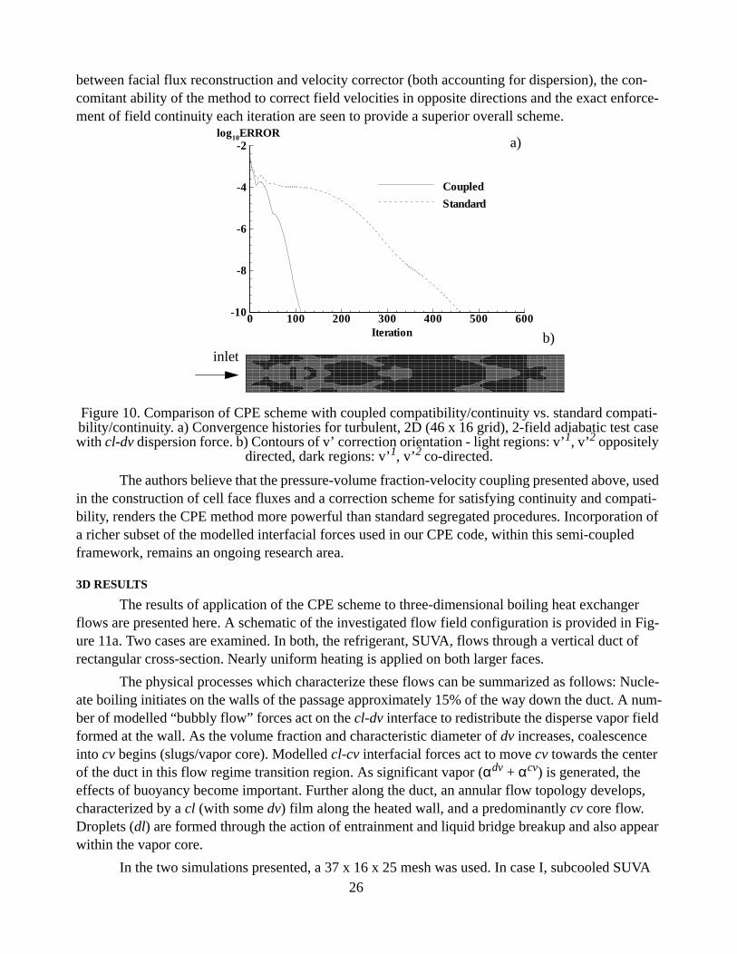
The superiority of the present scheme over the standard method is easily demonstrated even for relatively simple problems. For example, a turbulent, 2D, 2-field adiabatic duct flow was ana-lyzed. Only drag and turbulence dispersion interfacial forces were employed. A 46 x 16 mesh was uti-lized, the aspect ratio of the geometry was 500. Figure 10 shows the results of two runs for this flow field. The maximum obtainable convergence rate for the coupled scheme is seen to be significantly greater than that for the standard method. For this case, the CPE method required approximately 25% more CPU time per iteration than the standard method.

Figure 10b shows a contour plot distinguishing between regions where transverse velocity corrections were co-directed and oppositely directed at an interim iteration. As mentioned above, the standard pressure velocity coupling gives rise to co-directed field velocity corrections. In the coupled scheme, no relaxation was required for the field volume fraction equations. When the standard approach was used, the field volume fraction equations had to be underrelaxed. The consistency

∂p'/∂n 0= ∂α'/∂n 0=

A D T B+ +( ) PBJ D–1–

T B+( )≡,≡

D T B, , D T B, ,

φ ω– optD1–

T B+( )φnb 1 ωopt–( )φn

+ +=

b

25

between facial flux reconstruction and velocity corrector (both accounting for dispersion), the con-comitant ability of the method to correct field velocities in opposite directions and the exact enforce-ment of field continuity each iteration are seen to provide a superior overall scheme.

The authors believe that the pressure-volume fraction-velocity coupling presented above, used in the construction of cell face fluxes and a correction scheme for satisfying continuity and compati-bility, renders the CPE method more powerful than standard segregated procedures. Incorporation of a richer subset of the modelled interfacial forces used in our CPE code, within this semi-coupled framework, remains an ongoing research area.

3D RESULTS

The results of application of the CPE scheme to three-dimensional boiling heat exchanger flows are presented here. A schematic of the investigated flow field configuration is provided in Fig-ure 11a. Two cases are examined. In both, the refrigerant, SUVA, flows through a vertical duct of rectangular cross-section. Nearly uniform heating is applied on both larger faces.

The physical processes which characterize these flows can be summarized as follows: Nucle-ate boiling initiates on the walls of the passage approximately 15% of the way down the duct. A num-ber of modelled “bubbly flow” forces act on the cl-dv interface to redistribute the disperse vapor field formed at the wall. As the volume fraction and characteristic diameter of dv increases, coalescence into cv begins (slugs/vapor core). Modelled cl-cv interfacial forces act to move cv towards the center of the duct in this flow regime transition region. As significant vapor (αdv + αcv) is generated, the effects of buoyancy become important. Further along the duct, an annular flow topology develops, characterized by a cl (with some dv) film along the heated wall, and a predominantly cv core flow. Droplets (dl) are formed through the action of entrainment and liquid bridge breakup and also appear within the vapor core.

In the two simulations presented, a 37 x 16 x 25 mesh was used. In case I, subcooled SUVA

inlet

0 100 200 300 400 500 600-10

-8

-6

-4

-2

Iteration

log10ERROR

Coupled

Standard

Figure 10. Comparison of CPE scheme with coupled compatibility/continuity vs. standard compati-bility/continuity. a) Convergence histories for turbulent, 2D (46 x 16 grid), 2-field adiabatic test case with cl-dv dispersion force. b) Contours of v’ correction orientation - light regions: v’1, v’2 oppositely

directed, dark regions: v’1, v’2 co-directed.

a)

b)

26

enters the duct at a system pressure selected to provide partial dynamic similarity with a high pressure steam-water system. The heat flux applied is sufficient to give rise to an annular flow topolgy near the duct outlet. Figure 11a shows contours of the predicted field volume fractions at mid-duct and near-exit locations, illustrating the topological features described above.

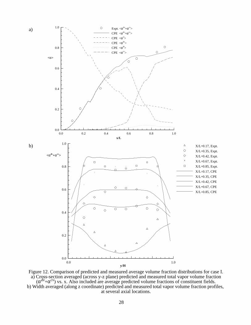
Quantitative comparisons for case I are provided in Figure 12. In Figure 12a, the axial distri-bution of predicted total vapor volume fraction (αdv + αcv) averaged across the duct (in y and z - refer to Figure 11a) is compared to gamma densitometer measurements. Also included in Figure 12a are the predicted section averaged volume fractions of the other constituent fields. (The “kinks” in the predictions arise from direct modelling of several unheated instrument ports which appear on the heated flats of the test section.) Agreement is very good between the measured and predicted average vapor volume fraction.

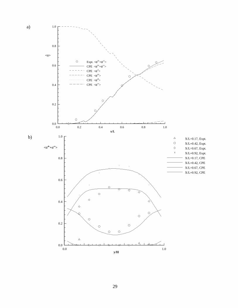
Case II is similar to case I except that the applied wall heat flux was reduced to approximately 0.6 of the case I flux. The resulting flow topology remains bubbly through the duct, just beginning to transition to annular flow at the duct outlet. This can be seen in Figure 13a, which shows the axial dis-

x

z

y

αcv

αcl

αdv

αdl*10

B 1.0

A 0.9

9 0.8

8 0.7

7 0.6

6 0.5

5 0.4

4 0.3

3 0.2

2 0.1

1 0.0

Figure 11. a) Schematic of 3D heated duct configuration. b) Case I predicted field volume fraction contours along plane in middle of duct, illustrating flow topology.

a)b)

annulartransitionbubbly

αcv

L

H

27

28

0.0 0.2 0.4 0.6 0.8 1.00.0

0.2

0.4

0.6

0.8

1.0

<α>

x/L

Expt. <αdv+αcv>

CPE <αdv+αcv>

CPE <αcl>

CPE <αdv>

CPE <αdl>

CPE <αcv>

0.0

0.2

0.4

0.6

0.8

1.0

1.00.0y/H

<αdv+αcv>

X/L=0.17, Expt.

X/L=0.35, Expt.

X/L=0.42, Expt.

X/L=0.67, Expt.

X/L=0.85, Expt.

X/L=0.17, CPE

X/L=0.35, CPE

X/L=0.42, CPE

X/L=0.67, CPE

X/L=0.85, CPE

Figure 12. Comparison of predicted and measured average volume fraction distributions for case I.a) Cross-section averaged (across y-z plane) predicted and measured total vapor volume fraction

(αdv+αcv) vs. x. Also included are average predicted volume fractions of constituent fields.b) Width averaged (along z coordinate) predicted and measured total vapor volume fraction profiles,

at several axial locations.

a)

b)

29

0.0 0.2 0.4 0.6 0.8 1.00.0

0.2

0.4

0.6

0.8

1.0

<α>

x/L

Expt. <αdv+αcv>

CPE <αdv+αcv>

CPE <αcl>

CPE <αdv>

CPE <αdl>

CPE <αcv>

0.0

0.2

0.4

0.6

0.8

1.0

1.00.0y/H

<αdv+αcv>

X/L=0.17, Expt.

X/L=0.42, Expt.

X/L=0.67, Expt.

X/L=0.92, Expt.

X/L=0.17, CPE

X/L=0.42, CPE

X/L=0.67, CPE

X/L=0.92, CPE

a)

b)

tribution of predicted and measured cross-sectionally averaged total vapor volume fraction. Local comparison of width averaged total vapor volume fraction profiles is provided in Figure 13b. For case II, pressure drop measurements were taken and are compared to prediction in Figure 13c. Comparison between prediction and measurement are good for all of these parameters.

CONCLUSIONS

A three-dimensional multi-field Coupled Phasic Exchange (CPE) algorithm, for the prediction of general two-phase flows has been presented. The focus of the paper was on six component numer-ical strategies which collectively characterize the CPE scheme. The scheme has been demonstrated to provide significant convergence improvement over standard methodologies. Each of the elements of the CPE scheme presented can be retrofit into existing segregated 2-fluid codes.

ACKNOWLEDGEMENTS

The authors acknowledge the contributions of Tom Trabold, Dave Considine and Bill Morris who provided the experimental SUVA data used for code comparisons.

REFERENCES

Briggs, W. L. (1987) A Multigrid Tutorial, SIAM.

0.0 0.2 0.4 0.6 0.8 1.0-2.0

-1.5

-1.0

-0.5

0.0

P-Pref (psi)

x/L

Expt.

CPE

Figure 13. Comparison of predicted and measured average volume fraction distributions for case II.a) Cross-section averaged (across y-z plane) predicted and measured total vapor volume fraction

(αdv+αcv) vs. x. Also included are average predicted volume fractions of constituent fields.b) Width averaged (along z coordinate) predicted and measured total vapor volume

fraction profiles, at several axial locations.c) Predicted and measured pressure drop along duct.

c)

30

Carver, M. B. (1984) “Numerical Computation of Phase Separation in Two Fluid Flow,” ASME Jour-nal of Fluids Engineering, Vol. 106, pp. 147-153.

Carver, M. B., Salcudean, M. (1986) “Three-Dimensional Numerical Modelling of Phase Distribution of Two-Fluid Flow in Elbows and Return Bends,” Numerical Heat Transfer, Vol. 10, pp. 229-251.

Clift, S. S., Forsyth, P. A. (1994) “Linear and Non-linear Iterative Methods for the Incompressible Navier-Stokes Equations,” Int. Journal for Numerical Methods in Fluids, Vol. 18, pp. 229-256.

DeBertadano, M. L., Lahey, R. T. Jr., Jones, O. T. (1994) “ Phase Distribution in Bubbly Two-Phase Flow in Vertical Ducts,” Int. Journal of Multiphase Flow, Vol. 20, No. 5, pp. 805-818.

Drew, D. A. (1992) “Analytical Modeling of Multiphase Flows,” from Boiling Heat Transfer, Ed. Lahey, Elsevier, pp. 31-84.

Gosman, A. D., Issa, R. Ii., Lekakou, C., Looney, M. K., Politis, S. (1992) “Multidimensional Model-ling of Turbulent Two-Phase Flows in Stirred Vessels,” AIChE Journal, Vol. 38, pp. 1853-1859.

Gu, C. Y. (1991) “Computation of Flows with Large Body Forces,” Proceedings of Conference on Laminar and Turbulent Flows, Stanford University, p. 1568-1578.

Huang, P. G., Leschziner, M. A. (1985) “Stabilization of Recirculating Flow Computations Performed with Second Moment Closure and Third Order Discretization,” Proceedings of the 5th Symposium on Turbulent Shear Flows, paper 20.7.

Hutchinson B. R., Raithby, G. D. (1986) “A Multigrid Method Based on the Additive Correction Strategy,” Numerical Heat Transfer, Vol.9, pp. 511-537.

Ishii, M. (1975) Thermo-Fluid Dynamic Theory of Two-Phase Flow, Eyrolles.

Issa, R. I., Oliviera, P. J. (1994) Numerical Prediction of Phase Separation in Two-Phase Flow Through T-Junctions,” Computers and Fluids, Vol. 23, No. 2, pp. 347-372.

Kelly, J. M., (1993) “A Four-Field Approach Towards Developing a Mechanistic Model for Mul-tiphase Flow,” Battelle, Pacific Northwest National Laboratories Report # PNL-SA--18878.

Kunz, R. F., Cope, W. K., Venkateswaran, S. (1997) “Stability Analysis of Implicit Multi-Fluid Schemes,” AIAA Paper AIAA-97-2080.

Lahey, R. T. (1996) “A CFD Analysis of Multidimensional Two-Phase Flow and Heat Transfer Phe-nomena,” from Process, Enhanced and Multiphase Heat Transfer, Ed. Manglik & Kraus, Begell House, pp. 431-441.

Lo, S. M. (1990) “Mathematical Basis of a Multi-Phase Flow Model, ARER Report 13432, Harwell Laboratory, United Kingdom.

Miller, T. F., Schmidt, F. W. (1988) “Use of a Pressure-Weighted Interpolation Method for the Solu-tion of the Incompressible Navier-Stokes Equations on a Non-staggered Grid System,” Numerical Heat Transfer, Vol. 14, pp. 213-233.

Patankar, S. V. (1980) Numerical Heat Transfer and Fluid Flow, Hemisphere.

Rhie, C. M., Chow, W. L. (1983) “Numerical Study of the Turbulent Flow Past an Airfoil with Trail-ing Edge Separation,” AIAA Journal, Vol. 21, pp. 1527-1532.

Serizawa, A., Kataoka, I., Michiyoshi, I. (1986) “Phase Distribution in Bubbly Flow, Data Set No. 24,” Proceedings of the Second International Workshop on Two-Phase Flow Fundamentals.

Settari, A., Aziz, K. (1973) “A Generalization of the Additive Correction Methods for the Iterative

31

Solution of Matrix Equations,” SIAM Journal of Numerical Analysis, Vol. 10, No. 3, pp. 506-521.

Shyy, W., Braaten, M. E. (1988) “Adaptive Grid Computation for Inviscid Compressible Flows Using a Pressure Correction Method, Proceedings of the First National Fluid Dynamics, Cincinatti.

Siebert, B. W., Antal, S. P. (1993) An IPSA-Based Two-Fluid Algorithm for Boiling Multi-Phase Flows, Proceeding of CFDS User’s Meeting.

Siebert, B. W., Maneri, C. C., Kunz, R. F., Edwards, D. P. (1995) “A Four-Field Model and CFD Implementation for Multi-Dimensional, Heated Two-Phase Flows,” Proceedings of the Second Inter-national Conference on Multiphase Flows, Kyoto.

Spalding, D. B. (1980) “Mathematical Methods in Nuclear-Reactor Thermal Hydraulics,” Keynote Paper, ANS Meeting on Nuclear-Reactor Thermal Hydraulics, Saratoga, NY.

Stewart, H. B., Wendroff, B. (1984) “Two-Phase Flow: Models and Methods,” Journal of Computa-tional Physics, Vol. 56, pp. 363-409.

Van Doormal, J. P., Raithby, G. D. (1984) “Enhancements of the SIMPLE Method for Predicting Incompressible Fluid Flows,” Numerical Heat Transfer, Vol. 7, pp. 147-163.

Van Doormal, Turan, A., J. P., Raithby, G. D. (1987) “Evaluation of New Techniques for the Calcula-tion of Internal Recirculating Flows,” AIAA Paper 87-0059.

Venkateswaran, S., Tamamidis, P., Merkle, C. L. (1997) “ Interpretation of Pressure-Based Methods as Time Marching Schemes,” Proceedings of 15th International Conference on Numerical Methods in Fluid Dynamics, Springer-Verlag Lecture Series in Physics.

APPENDICES: ELEMENTS OF ADDITIVE CORRECTION STABILITY ANALYSIS

Appendix A: Fourier Stability for Additive Correction

Assuming periodicity in x and y, the discrete Fourier transform of equation 25 can be written:

(A.1)

where l, m correspond to integer Fourier mode numbers ( ). Since q is a function

of index i only, for m > 0, therefore only pure axial modes can be influenced by the 1D

AC procedure. To examine the influence of AC on these axial modes, consider equation 26 written as:

(A.2)

where . Again assuming periodicity in y:

p'n+1

lmp'ˆ

lmq

lm+=

0 l ni 0 m nj≤ ≤,≤ ≤

q

lm0=

nj 1 2K2–( )qi K1– qi+1 qi-1+( )+[ ] K1 p'ˆ i+1,j p'ˆ i-1,j+( ) K2 p'ˆ i,j+1 p'ˆ i,j-1+( ) Sij–+[ ] p'ˆ i j,–{ }

j=1

nj

∑=

K1

ν1

2 ν1 ν2+( )-------------------------- K2,ν2

2 ν1 ν2+( )--------------------------= =

32

(A.3)

Substituting A.3 into A.2 and Fourier transforming in x and y†:

(A.4)

where, kl and km designating the wave numbers associated with axial modes l and m. Considering only the m = 0 mode, Equation A.4 reduces to:

(A.5)

Defining the amplification factor for the entire scheme as:

(A.6)

Considering pure axial modes and substituting equation A.5:

(A.7)

Showing that BC identically damps pure axial modes.

†. Source term Sij can be neglected in the stability analysis by considering transformed variables to be errors from exact solution to difference equation.

p’ˆ i j,

j=1

nj

∑ p'ˆ i,j+1

j=1

nj

∑ p'ˆ i,j-1

j=1

nj

∑= =

q

lme

Ikm

j∆ynj 1 2K2– 2K1 k

l∆x( )cos–[ ]

1 2K2– 2K1 kl∆x( )cos–[ ] p'ˆ

lmj=1

nj

∑–=

1 2K2– 2K1 kl∆x( )cos–[ ] p'ˆ

lme

Iklj∆y

nj

∑–=

q

l0nj{ } p’ˆ

l0j=1

nj

∑– nj{ } p'ˆ

l0–= =

glm

p’n 1+

lm

p’n

lm

-------------------------p’ˆ

lm

p'n

lm

---------------------q

lm

p'n

lm

---------------------+ glmJACOBI

1q

lm

p'ˆ

lm

----------------+

= = =

gl0 gl0JACOBI

1q

l0

p’ˆ

l0

---------------+

0= =

33

34

Appendix B: Results of 3D Stability of Anisotropic Diffusion Equation for Type II and Type II Cells

In three dimensions, application of the MSJ scheme to equation 22 yields:

(A.1)If a VonNeumann stability analysis is applied to equation A.8, the results in Figure A.1 are

obtained. In Figure A.8a, stability results are shown for ν2/ν1 = ν2/ν3 = 10000, corresponding to Type

II cells characterized by ∆x/∆y = ∆z/∆y = 100 (refer Figure 5). In Figure A.8b, results are shown for ν2/ν1 = 100000, ν2/ν3 = 100, corresponding to Type III cells characterized by ∆x/∆y = 100, ∆z/∆y =

10.

For Type II cells, the MSJ scheme exhibits poor damping (|g| ≅ 1) only for purely axial modes, 0 ≤ φx ≤ π, φy = φz = 0. For Type III cells, the MSJ scheme exhibits poor damping for pure x-z modes,

0 ≤ φx ≤ π, φy = 0, 0 ≤ φz ≤ π.

p’i,j,kk+1

ωk

2 ν1 ν2 ν3+ +( )-------------------------------------- ν1 p’i+1,j,k

kp’i-1,j,k

k+( ) ν2 p’i,j+1,k

kp’i,j-1,k

k+( ) ν3 p’i,j,k+1

kp’i,j,k-1

k+( )+ +[ ]

1 ω–( )p'i,jk

+

=

k 0 1 2 3 ω1, , , 0.528 ω2, 0.878 ω3, 4.040= = = =

p'ˆ i,j,k p'i,j,k 3

p'i,j,k0

p'i,j,kn

=,=

35

0 π π π

π

0

0

0

φz=0

φz=πφz=7π/8φz=6π/8

φz=5π/8φz=4π/8φz=3π/8

φz=2π/8φz=π/8

φx φx φx

φy

φy

φy

0 0

π

π

1.00

0.90

0.80

0.70

0.60

0.50

0.40

0.30

0.20

0.10

0.00

0 π π π

π

0

0

0

φz=0

φz=πφz=7π/8φz=6π/8

φz=5π/8φz=4π/8φz=3π/8

φz=2π/8φz=π/8

φx φx φx

φy

φy

φy

0 0

π

π

1.00

0.90

0.80

0.70

0.60

0.50

0.40

0.30

0.20

0.10

0.00

|g|

|g|

TYPE II Cells

TYPE III Cells

Figure A1. Results of VonNeumann analysis for model diffusion equation.