A Coupled Vegetation–Crust Model for Patchy Landscapes

SHAI KINAST,1 YOSEF ASHKENAZY,1 and EHUD MERON1,2

Abstract—A new model for patchy landscapes in drylands is

introduced. The model captures the dynamics of biogenic soil

crusts and their mutual interactions with vegetation growth. The

model is used to identify spatially uniform and spatially periodic

solutions that represent different vegetation-crust states, and map

them along the rainfall gradient. The results are consistent exten-

sions of the vegetation states found in earlier models. A significant

difference between the current and earlier models of patchy land-

scapes is found in the bistability range of vegetated and

unvegetated states; the incorporation of crust dynamics shifts the

onset of vegetation patterns to a higher precipitation value and

increases the biomass amplitude. These results can shed new light

on the involvement of biogenic crusts in desertification processes

that involve vegetation loss.

1. Introduction

Water-limited vegetation landscapes are usually

patchy (VALENTIN et al. 1999; DEBLAUWE et al. 2008).

Vegetation patch formation is a means by which

dryland vegetation copes with water stress. The for-

mation of patches devoid of vegetation provides

additional sources of water to adjacent vegetation

patches through various mechanisms of water trans-

port, which help the vegetation to sustain itself. Self-

organized vegetation patchiness of this kind is cur-

rently viewed as a symmetry-breaking pattern

formation phenomenon driven by positive feedbacks

between two main processes: local vegetation growth

and water transport toward the growing vegetation.

Several water-transport forms have been identified,

including overland water flow, water conduction by

laterally extended root zones, soil-water diffusion,

and fog advection (RIETKERK and VAN DE KOPPEL 2008;

MERON 2012; KINAST et al. 2014; BORTHAGARAY et al.

2010; BORGOGNO et al. 2009). The mechanism by

which local vegetation growth enhances water

transport toward patches of growing vegetation

depends on the type of water transport. We focus here

on overland water flow as a major type of water

transport in dryland landscapes.

Soil areas devoid of vegetation are often covered

by thin biogenic soil crusts (WEST 1990). Depending

on the precipitation regime, soil characteristics, and

disturbances, these crusts may consist of one or more

organisms, including cyanobacteria, green algae,

fungi, lichens, and mosses. Soil crusts reduce soil

erosion by water and wind. They also provide a

source of carbon and nitrogen for vascular plants.

Most important to our discussion here is their capa-

bility to induce overland water flow (runoff) by

changing the rate of surface-water infiltration into the

soil. Crusts that are dominated by cyanobacteria, for

example, can absorb water several times their dry

weight in only a few seconds (CAMPBELL 1979). This

results in crust swelling and soil-pore blocking and,

consequently, in significant reduction of water infil-

tration shortly after rain starts (VERRECCHIA et al.

1995; ELDRIDGE et al. 2012). Because cyanobacteria

are photosynthetic organisms, their growth is hin-

dered by vegetation, which limits exposure to

sunlight. The reduced infiltration in crusted areas and

the absence of crusts in vegetated areas result in an

infiltration contrast: low infiltration rates in sparsely

vegetated areas and high rates in densely vegetated

areas. Additional factors contributing to this outcome

include soil mounds generated by dust deposition

(SHACHAK and LOVETT 1998) and higher soil porosity

in vegetation patches (PUIGDEFABREGAS 2003; STAVI

et al. 2009). The infiltration contrast induces overland

1 Department of Solar Energy and Environmental Physics,

Blaustein Institutes for Desert Research, Ben-Gurion University of

the Negev, 84990 Sede Boqer Campus, Israel. E-mail:

shaikinast@gmail.com2 Department of Physics, Ben-Gurion University of the

Negev, 84105 Beer Sheva, Israel.

Pure Appl. Geophys. 173 (2016), 983–993

� 2014 Springer Basel

DOI 10.1007/s00024-014-0959-8 Pure and Applied Geophysics

water flow toward densely vegetated areas, which

accounts for the enhancement of water transport by

local vegetation growth, and closes the positive

feedback loop (vegetation growth ! water transport

! vegetation growth) that drives vegetation pattern

formation (hereafter the ‘‘infiltration feedback’’).

Mathematical models that incorporate infiltration

feedback into the model’s equations (RIETKERK et al.

2002; GILAD et al. 2004, 2007) indeed capture a

nonuniform stationary instability of uniform vegeta-

tion that gives rise to periodic vegetation patterns.

These models capture the effect of biogenic crusts on

vegetation pattern formation implicitly by introduc-

ing an infiltration-contrast parameter that quantifies

the differences between infiltration rates in vegetated

and unvegetated areas. This modeling approach,

however, ignores the properties and dynamics of the

biogenic crust, which limits the applicability of the

models in two main respects. First, different types of

biogenic crust are present in nature; ignoring their

properties severely limits the ability to distinguish

between the effects of different crust types on vege-

tation pattern formation (YAIR et al. 2011). The

second respect is related to the absence of competi-

tion for space between biogenic crusts and

vegetation. It is well established (PRASSE and BORN-

KAMM 2000) that crusts can suppress vegetation

growth by preventing seed germination. This effect

may be important in desertification processes,1 for

example shrubland–crustland transitions, an example

of which is shown in Fig. 1; rapid soil coverage by

crusts after degradation of the woody vegetation may

delay or even prevent vegetation regrowth.

In the work discussed in this paper we studied the

effect of biogenic soil crusts on vegetation pattern

formation by adding an equation for crust dynamics

to an earlier vegetation model (GILAD et al. 2007),

and modifying the remaining model equations to take

into account the coupled crust–vegetation dynamics

and crust–water dynamics. We note that models of

crust dynamics have been proposed and studied

elsewhere (BAR et al. 2002; MANZONI et al. 2014;

KINAST et al. 2013). To the best of our knowledge,

however, the coupling between vegetation dynamics

and crust dynamics in a spatial context has not yet

been studied.

We first show that the new crust–vegetation

model reproduces the sequence of vegetation states

along the rainfall gradient that have been predicted by

earlier vegetation models. We then present additional

predictions that emphasize the effect of crust

dynamics in the development of vegetation.

2. A Crust–Vegetation Model

The new crust–vegetation model we propose

consists of four dynamic variables, representing the

areal densities of vegetation biomass (B), crust bio-

mass (C), soil water (W), and surface water (H), all

having the dimensions mass per unit area. The model

is based on a simplified version (KINAST et al. 2014)

of the vegetation model introduced by GILAD et al.

(2004, 2007). The model’s equations are:

BT ¼ GBBð1�B=KBÞ�MBB� /BBC

ðBþB0Þm þDBr2B ;

ð1aÞ

CT ¼ GCCð1 � C=KCÞ � MCC � /CCB þ DCr2C ;

ð1bÞ

WT ¼ IH � Nð1 � RB=KBÞW � GW W þ DWr2W ;

ð1cÞ

1 Desertification is defined as an irreversible reduction in

biological productivity (biomass production rate) as a result of

climate fluctuations or anthropogenic disturbances.

Figure 1Degraded landscape in the Northern Negev (Israel) after a series of

droughts. The white patches consist of shells of dead snails that

used to feed on dead branches of living shrubs, and constitute a

‘‘ghost pattern’’ of a former vegetation spot pattern. From SHACHAK

(2011) (with permission)

984 S. Kinast et al. Pure Appl. Geophys.

HT ¼ P � IH � GHH �r � J ; ð1dÞ

where,

GB ¼ KBWð1 þ EBÞ2 ; ð2aÞ

GC ¼ KCW W þ KCHH ; ð2bÞ

GW ¼ CBBð1 þ EBÞ2 þ CCW C ; ð2cÞ

GH ¼ CCHC ; ð2dÞ

I ¼ A�fCC þ QC

C þ QC

��B þ QBfB

B þ QB

�; ð2eÞ

J ¼ �DHHbrH : ð2fÞ

We assume in this model that the vegetation and the

biogenic crust are both characterized by logistic

growth and linear mortality. The ‘‘carrying capacity’’

KB represents genetic constraints, such as stem

architecture and strength, whereas KC mainly repre-

sents constraints of exposure to sunlight. The growth

rates GB and GC both depend on water availability

but assume different functional forms. Plants exploit

below-ground water (W) through water uptake by

their roots. This is accounted for by Eq. (2a), where E

is a measure for the root-to-shoot ratio and relates

root size to above-ground biomass B. The particular

biomass dependence of the growth rate GB follows

from the assumption of confined root zones (ZELNIK

et al. 2013). The crust exploits both below-ground

and above-ground water, hence the form of Eq. (2b).2

For the same reason the equations for W and H both

contain terms describing water uptake by the crust

(CCW CW in GW and CCHCH in GH , respectively).

The vegetation and the biogenic crust compete

indirectly by consumption of the common water

resource, and directly by competition for space.

Plants can suppress the growth of biogenic crusts by

spreading litter that limits sunlight. Plants can also

destroy biogenic crusts if the litter is toxic (BOEKEN

AND ORENSTEIN 2001). These effects are represented

by the parameter /C in Eq. (1b). Biogenic crusts

suppress the growth of vegetation by preventing seed

seeding and germination (PRASSE and BORNKAMM

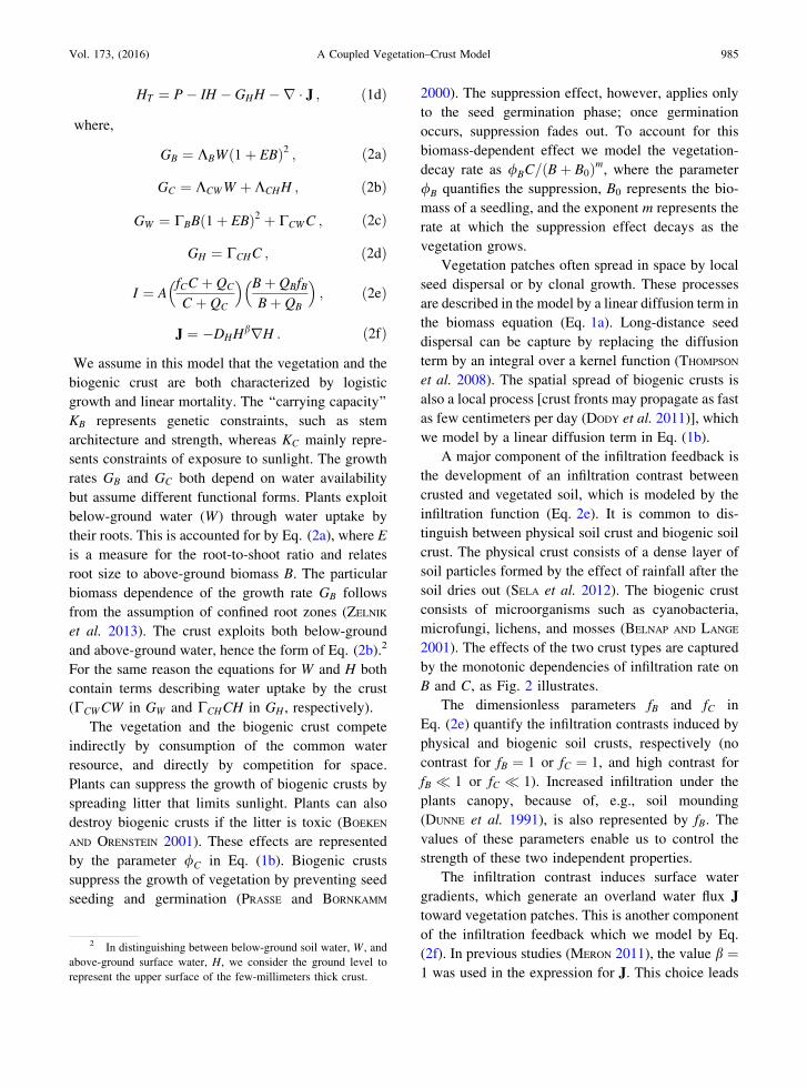
2000). The suppression effect, however, applies only

to the seed germination phase; once germination

occurs, suppression fades out. To account for this

biomass-dependent effect we model the vegetation-

decay rate as /BC=ðB þ B0Þm, where the parameter

/B quantifies the suppression, B0 represents the bio-

mass of a seedling, and the exponent m represents the

rate at which the suppression effect decays as the

vegetation grows.

Vegetation patches often spread in space by local

seed dispersal or by clonal growth. These processes

are described in the model by a linear diffusion term in

the biomass equation (Eq. 1a). Long-distance seed

dispersal can be capture by replacing the diffusion

term by an integral over a kernel function (THOMPSON

et al. 2008). The spatial spread of biogenic crusts is

also a local process [crust fronts may propagate as fast

as few centimeters per day (DODY et al. 2011)], which

we model by a linear diffusion term in Eq. (1b).

A major component of the infiltration feedback is

the development of an infiltration contrast between

crusted and vegetated soil, which is modeled by the

infiltration function (Eq. 2e). It is common to dis-

tinguish between physical soil crust and biogenic soil

crust. The physical crust consists of a dense layer of

soil particles formed by the effect of rainfall after the

soil dries out (SELA et al. 2012). The biogenic crust

consists of microorganisms such as cyanobacteria,

microfungi, lichens, and mosses (BELNAP AND LANGE

2001). The effects of the two crust types are captured

by the monotonic dependencies of infiltration rate on

B and C, as Fig. 2 illustrates.

The dimensionless parameters fB and fC in

Eq. (2e) quantify the infiltration contrasts induced by

physical and biogenic soil crusts, respectively (no

contrast for fB ¼ 1 or fC ¼ 1, and high contrast for

fB � 1 or fC � 1). Increased infiltration under the

plants canopy, because of, e.g., soil mounding

(DUNNE et al. 1991), is also represented by fB. The

values of these parameters enable us to control the

strength of these two independent properties.

The infiltration contrast induces surface water

gradients, which generate an overland water flux J

toward vegetation patches. This is another component

of the infiltration feedback which we model by Eq.

(2f). In previous studies (MERON 2011), the value b ¼1 was used in the expression for J. This choice leads

2 In distinguishing between below-ground soil water, W , and

above-ground surface water, H, we consider the ground level to

represent the upper surface of the few-millimeters thick crust.

Vol. 173, (2016) A Coupled Vegetation–Crust Model 985

to a nonlinear diffusion term in Eq. (1d) proportional

to r2H2 (GILAD et al. 2007). Here we choose the

value b ¼ 0, which leads to a linear diffusion term,

DHr2H, and simplifies numerical studies of the

model’s equations. Linear diffusion does not capture

the compact nature of overland water flow, but we

verified that our results do not depend crucially on

this detail. This is in accordance with VAN DER STELT

et al. (2013), who observed that nonlinear water

diffusion does not have a crucial qualitative effect on

the results of a similar model of patterned vegetation.

Assuming unsaturated soil, water transport below

ground level is also considered to be a linear diffu-

sion process (DWr2W). Fast soil-water transport in

comparison with vegetation spread, with strong

uptake, constitute another type of pattern-forming

feedback, which can induce vegetation patterns by a

Turing instability (KINAST et al. 2014).

The remaining factors affecting water dynamics

are rainfall, represented by the precipitation rate P,

and evaporation of soil water at a rate

Nð1 � RB=KBÞ, which takes into account reduced

evaporation by shading. The numerical values we use

for all model parameters are given in Table 1.

It proves beneficial to study the model equations

using non-dimensional variables and parameters,

which enables us to eliminate redundant parameters.

The non-dimensional quantities we use are defined in

Table 2. The non-dimensional model equations read:

bt ¼ gbbð1 � bÞ � b � ubbc

ðb þ b0Þm þr2b ð3aÞ

ct ¼ gccð1 � cÞ � lc � uccb þ dcr2c ð3bÞ

wt ¼ Ih � mð1 � rbÞw � gww þ dwr2w ð3cÞ

ht ¼ p � Ih � ghh þ dhr2h ð3dÞ

where:

gb ¼ mwð1 þ gbÞ2 ð4aÞ

gc ¼ mðkcww þ kchhÞ ð4bÞ

gw ¼ cbbð1 þ gbÞ2 þ ccwc ð4cÞ

gh ¼ cchc ð4dÞ

I ¼ a�fcc þ qc

c þ qc

��b þ qbfb

b þ qb

�ð4eÞ

3. Vegetation-Crust States Along the Rainfall

Gradient

Earlier vegetation models that capture overland

water flow (RIETKERK et al. 2002; GILAD et al. 2004,

2007), predict five basic vegetation states along the

rainfall gradient; uniform vegetation, gap patterns,

stripe or labyrinthine patterns, spot patterns, and bare

soil. The models further predict bistability ranges

B/KB

I (yr

−1 )

C/KC

I (yr

−1)

A

AfB

A

AfC

QB/K

BQ

C/K

C

cut of I(B,C) at C=0 cut of I(B,C) at B=0(a) (b)

Figure 2Cuts of the infiltration rate function I ¼ IðB;CÞ (Eq. 2e) at C ¼ 0 (a), showing the dependence of the infiltration rate on the proportional

vegetation biomass B=K, and at B ¼ 0 (b), showing the dependence of the infiltration rate on the proportional crust biomass C=K. The

infiltration contrast between bare and vegetated soil (because of the physical crust) is quantified by fB, and the contrast between bare and

crusted soil is quantified by fC , where 0�ffB; fCg� 1. Low values of fB or fC represent high infiltration contrasts

986 S. Kinast et al. Pure Appl. Geophys.

between any pair of consecutive vegetation states,

which result in a wide variety of non-periodic pat-

terned states (MERON 2012). These predictions agree

well with observations (DEBLAUWE et al. 2008), and

therefore provide an important test for the new veg-

etation-crust model proposed here. To discover what

states along the rainfall gradient the model equations

(Eqs. 3a–3d) predict, we studied stationary solutions

in one spatial dimension, using a numerical contin-

uation method and linear stability analysis, and

complemented this analysis with direct numerical

integration of the model’s equations in one and two

spatial dimensions, as described below. In both cases

we assumed that the development of an infiltration

contrast between vegetated and unvegetated areas is

because of biogenic crusts only, by choosing

fb ¼ 1; fc ¼ 0:1.

Figure 3 shows bifurcation diagrams for station-

ary solutions of Eqs. (3a–3d) in one spatial

dimension, and displays the maximum values of the

vegetation biomass (Fig. 3a) and of the crust biomass

(Fig. 3b) as functions of precipitation rate.

Four types of stable uniform solutions can be dis-

tinguished. The first is a constant solution that

describes bare-soil devoid of vegetation and crust, B(b ¼ 0; c ¼ 0). It exists for all precipitation values but

is stable only for 0\p\p0. At p ¼ p0 the bare-soil

solution loses stability to another constant solution

devoid of vegetation that describes uniform crust, C(b ¼ 0; c 6¼ 0). This solution is stable up to p ¼ p2

Table 1

Model parameters: their symbols, descriptions, units, and values used in this study

Parameters Description Units Value

KB Vegetation growth rate (kg/m2)-1 year-1 0.032

E Root augmentation per unit biomass of vegetation (kg/m2)-1 1.5

KB Maximum standing biomass of vegetation (carrying capacity) kg/m2 1

MB Vegetation mortality rate year-1 1.2

/B Vegetation suppression by crust year-1 1

B0 Vegetation biomass reference value beyond which the suppression

by crust approaches its minimum

kg/m2 0.05

m Steepness of suppression of competition term by vegetation – 1

KCW Crust growth rate as a result of uptake of soil water (kg/m2)-1 year-1 0.035

KCH Crust growth rate as a result of uptake of surface water (kg/m2)�1 year�1 0.01

KC Maximum crust biomass (carrying capacity) kg/m2 0.003

MC Crust mortality rate year�1 0.2

/C Crust suppression by vegetation year�1 20

A Maximum infiltration rate in uncrusted soil year�1 10

QB Vegetation biomass reference value beyond which infiltration rate

under a vegetation patch approaches its maximum

kg/m2 0.05

QC Crust biomass reference value beyond which infiltration rate under

a crust patch approaches its minimum

kg/m2 0.0006

fB Infiltration contrast between bare soil and vegetated soil – 1

fC Infiltration contrast between bare soil and crusted soil – 0.1

N Soil water evaporation rate year�1 4

R Evaporation reduction due to shading – 0.95

P Mean annual precipitation rate kg/m2year�1 (0, 500)

CB Soil water consumption rate per unit vegetation biomass (kg/m2)�1year�1 30

CCW Soil water consumption rate per unit crust biomass (kg/m2)�1year�1 0.1

CCH Surface water consumption rate per unit crust biomass (kg/m2)�1year�1 0.02

DB Vegetation seed dispersal coefficient m2/year 6:25 � 10�4

DC Crust spores dispersal coefficient m2/year 6:25 � 10�3

DW Transport coefficient for soil water m2/year 6:25 � 10�2

DH Bottom friction coefficient between surface water and ground surface m2/year 5

The values of the parameters appearing in the equations for vegetation biomass (B), the soil water (W), and the surface water (H) are taken

from GILAD et al. (2007). The values for the crust (C) equation are based on BELNAP and LANGE (2001), GARCIA-PICHEL et al. (2003), PRASSE and

BORNKAMM (2000), ZAADY and SHACHAK (1994), and BOEKEN and ORENSTEIN (2001). The units of mean annual precipitation rate (P) are

equivalent to mm/year

Vol. 173, (2016) A Coupled Vegetation–Crust Model 987

where it bifurcates to a constant mixed vegetation–

crust solution, M (b 6¼ 0; c 6¼ 0). The mixed solution

branch terminates (as a physical solution) at p ¼ p3 on

a constant solution branch that describes uniform

vegetation devoid of crust, V (b 6¼ 0; c ¼ 0). The

mixed solution M, however, is unstable to the growth

of nonuniform perturbations, which leads to a non-

uniform solution branch, P (b 6¼ 0; c 6¼ 0), describing

a periodic mixed pattern of vegetation and crust (Fig.

4). The periodic solution branch P emanates from the

constant solution M very close to p ¼ p2 and returns

to M very close to p ¼ p3. Because both bifurcations

are subcritical, the stable part of the periodic solution

branch P occupies a wider precipitation range boun-

ded by two fold bifurcations at p1 and at p4. This range

includes a bistability subrange, p1\p\p2, with the

uniform crust solution C, and a bistability subrange,

p3\p\p4, with the uniform vegetation solution V.

Altogether the following sequence of stable states

has been found along the rainfall gradient in one spa-

tial dimension: uniform vegetation V (p[ p3),

periodic spatial patternP (p1\p\p4), uniform crust C(p0\p\p2) and bare soilB (0\p\p0). An additional

finding is the existence of two bistability ranges:

1 uniform vegetation and periodic patterns; and

2 uniform crust and periodic patterns.

These results are consistent with those obtained in

the earlier models when associating the bare-soil

solution B and the crust solution C with the ‘‘bare-soil

state’’ of the earlier models.

Figure 4 shows typical spatial profiles of periodic

solutions, obtained by numerical integration of Eqs.

(3a–3d) in one spatial dimension, at two precipitation

values, p ¼ 1 and p ¼ 2, located near the low-pre-

cipitation and high-precipitation edges of the periodic

(a) (b)

Figure 3Bifurcation diagram for stationary solutions of the vegetation-crust model. Shown are the maximum values of the vegetation biomass b (a)

and of the crust biomass c (b) as functions of precipitation rate p. Solid lines represent stable solutions and dashed (dotted) lines represent

unstable solutions to uniform (nonuniform) perturbations. Five distinct solutions are denoted: bare soil B, uniform crust C, uniform mixture of

vegetation and crust M, uniform vegetation V, and periodic vegetation-crust pattern P. The latter emanates from M and returns to M very

close to the bifurcation points where M connects to C (p ¼ p2) and to V (p ¼ p3). The insets show magnifications of the neighborhoods of

these bifurcation points. Not shown in the bifurcation diagrams are negative solutions, which represent unphysical states. Parameter values are

as given in Table 1

Table 2

Relations between non-dimensional variables and parameters and

dimensional variables and parameters appearing in the dimen-

sional form of the model Eqs. (1a–1d)

Quantity Scaling Quantity Scaling

b B=KB a A=MB

c C=KC qc QC=KC

w KBW=N qb QB=KB

h KBH=N fc fCm N=MB fb fBg EKB r R

b0 B0=KB cb CBKB=MB

ub /BKC=MBKmB ccw CCW KC=MB

uc /CKB=MB cch CCHKC=MB

kCW KCW=KB p KBP=NMB

kCH KCH=KB dc DC=DB

l MC=MB dw DW=DB

t MBT dh DH=DB

x XffiffiffiffiffiffiffiffiffiffiffiffiffiffiffiMB=DB

p

988 S. Kinast et al. Pure Appl. Geophys.

solution branch depicted in Fig. 3. At p ¼ 1 the

solution appears as vegetation spots surrounded by

crusted soil (Fig. 4a, c), whereas at p ¼ 2 the solution

appears as crust gaps in vegetated soil (Fig. 4b, d).

The remaining parts of this figure show the associated

spatial profiles of the soil–water and surface–water

variables. As Fig. 4e, f show, the minima of soil

water content (w) coincide with maxima of vegeta-

tion biomass (b) because of the high uptake rate gw.

Figure 4g, h show that the maxima of surface-water

0

0.1

0.2b

0

0.5

1

c

0.22

0.24

0.26

w

0 1 2 3 4 5

0.25

0.3

0.35

0.4

h

x/100

0 1 2 3 4 5

x/100

p=1 p=2

(a) (b)

(c) (d)

(e) (f)

(g) (h)

Figure 4Spatially periodic solutions of Eqs. (3a–3d) in one spatial dimension. Shown are the spatial profiles of all dynamic variables at low

precipitation (a, c, e, g) and at high precipitation (b, d, f, h). Parameter values are as given in Table 1

Vol. 173, (2016) A Coupled Vegetation–Crust Model 989

height (h) coincide with the maxima of crust biomass

(c). This can be understood from Eq. (4e), because

infiltration of surface water is a monotonically

decreasing function of crust biomass, as shown by

Fig. 2b.

In two spatial dimensions, previous models pre-

dicted three basic types of periodic solutions,

representing hexagonal spot patterns at relatively low

precipitation, stripes (labyrinthine) patterns at inter-

mediate precipitation, and hexagonal gap patterns at

relatively high precipitation. These three patterned

vegetation states are also found by numerical inte-

gration of Eqs. (3a–3d), as shown by Fig. 5. Shown

are the time evolution of the same initial conditions at

increasing precipitation values and the asymptotic

approach to hexagonal-spot, stripe, and hexagonal-

gap patterns.

4. The Significance of Modeling Crust Dynamics

The vegetation-crust model (Eqs. 3a–3d) not only

reproduces the main qualitative behaviors found in

previous models, but also provides new insights.

Figure 6 shows a comparison of the bifurcation dia-

gram presented in Fig. 3a with the corresponding

diagram of a reduced model, obtained by setting the

growth rate of the crust variable to zero (gc ¼ 0),

choosing fb ¼ 0:1, and leaving all other parameters

unchanged. The right hand side of the crust equation

(Eq. 3b) includes then the negative terms only, which

drive the crust biomass to zero and reduce the four-

variable vegetation-crust model (Eqs. 3a–3d) to a

three-variable vegetation model. The latter coincides

with a simplified version of the Gilad et al. model

(2007) studied earlier (ZELNIK et al. 2013).

y/10

0

6

4

2

0

y/10

0

6

4

2

0

y/10

0

6

4

2

0

x/100

0 2 4 6

x/100

0 2 4 6

x/100

y/10

0

0 2 4 6

6

4

2

0

0

0.05

0.1

0.15

0.2

p=1.1 p=1.8 p=2.1

bt=0

t=50

t=1000

t=20000

Figure 5Three basic types of asymptotic vegetation–crust patterns. Shown are snapshots of three simulations of Eqs. (3a–3d) at increasing precipitation

values, starting from the same initial condition. At p ¼ 1:1 the dynamics converge to a spot pattern, at p ¼ 1:8 to stripe patterns, and at

p ¼ 2:1 to a gap pattern. Darker shades represent higher vegetation biomass (b). The crust biomass forms an anti-phase pattern, occupying the

light-shade areas that are devoid of vegetation. Parameter values are as given in Table 1

990 S. Kinast et al. Pure Appl. Geophys.

The bifurcation diagram of the vegetation-crust

model (Fig. 6b) differs from that of the vegetation

model (Fig. 6a) in several structural respects:

1 it contains the additional solution branches C and

M;

2 the periodic solution P is a mixed vegetation-crust

solution; and

3 the periodic solution emanates from and returns to

the (unstable) uniform mixed state solution branch

M (rather than the uniform vegetation solution).

Note that the spatial profiles of the vegetation (b)

and of the crust (c) along the periodic solution branch

are anti-phase, as shown by Fig. 4; that is, maxima of

b correspond to minima of c and vice versa.

More significant from an ecological perspective

are two quantitative differences related to the fold

bifurcation at p ¼ p1 at which the stable periodic

state P appears. Including crust dynamics shifts this

bifurcation point to higher precipitation and biomass

values. The shift to a higher precipitation rate

increases the range of the unproductive state, B or C,

at the expense of the productive vegetation-pattern

state P, whereas the shift to higher biomass values

increases the attraction basin of the unproductive

state within its bistability range with the productive

vegetation-pattern state. These results suggest that

incorporating crust dynamics in vegetation models

can be highly significant for studying state transitions

involving vegetation loss or vegetation recovery. The

inclusion of dynamic crust also shifts p ¼ p4 to a

higher value, implying the persistence of vegetation

gap patterns at higher precipitation rates and a wider

bistability range of vegetation gap patterns and uni-

form vegetation.

5. Conclusions

A new model for patchy water-limited landscapes

has been introduced. Unlike earlier models, in which

soil-crust effects are considered in a parametric way,

through a biomass-dependent infiltration rate, the

new model captures the actual dynamics of biogenic

soil crusts and their mutual interactions with vege-

tation growth. Using the model we mapped the

vegetation-crust states along the precipitation axis

and found them to be consistent extensions of the

results of previous models. We further emphasized

significant differences between the new and earlier

models in the bistability range of productive and

unproductive states; taking into account crust

dynamics shifts the fold-bifurcation point at which

stable vegetation patterns appear to higher precipita-

tion and biomass values.

These differences can be attributed in part to the

competition term in Eq. (3a), which models the

suppression effects that biogenic crusts exert on

vegetation growth by slowing seed germination. The

suppression effect and its fadeout as vegetation

grows, depend on the parameter /B, m and B0. Fur-

ther studies are needed to clarify how these

(a) (b)

Figure 6Comparison between bifurcation diagrams with (b) and without (a) a dynamic crust, both showing the vegetation biomass (b) as a function of

precipitation (p). Solid (dashed) lines represent stable (unstable) solutions. Addition of a dynamic crust shifts the fold bifurcation point,

p ¼ p1, to higher precipitation and biomass values. Along with these shifts the unstable branch of the periodic vegetation solution P shifts

upward. Parameter values are as given in Table 1, except for fb ¼ 0:1; fc ¼ 1; kCW ¼ kCH ¼ 0 in (a)

Vol. 173, (2016) A Coupled Vegetation–Crust Model 991

parameters affect the stable and unstable branches of

the periodic solution P.

The vegetation-crust model (Eqs. 3a–3d) may

shed new light on the effects of biogenic crusts on the

response of dryland ecosystems to rainfall variability,

and may improve understanding of desertification

processes, such as that shown in Fig. 1, and of means

to facilitate recovery to the original state. To this end

model studies with periodic or stochastic precipita-

tion to simulate successive droughts should be

conducted.

Acknowledgments

We wish to thank Golan Bel, Jost von-Hardenberg,

Eli Zaady and Yuval Zelnik for helpful discussions.

The research leading to these results has received

funding from the Israel Science Foundation (Grant

Numbers 75/12 and 305/13).

REFERENCES

A. ANA I. BORTHAGARAY, M. A. FUENTES, and P. A. MARQUET.

Vegetation pattern formation in a fog-dependent ecosystem.

Journal of Theoretical Biology, 265:18–26, 2010.

M. BAR, J. HARDENBERG, E. MERON, and A. PROVENZALE. Modelling

the survival of bacteria in drylands: the advantage of being

dormant. Proceedings of the Royal Society of London. Series B:

Biological Sciences, 269(1494):937–942, 2002.

J. BELNAP and O. L. LANGE. Biological Soil Crusts: Structure,

Function, and Management. Springer, 2001.

B. BOEKEN and D. ORENSTEIN. The effect of plant litter on ecosystem

properties in a Mediterranean semi-arid shrubland. J. Veg. Sci.,

12:825–832, 2001.

F. BORGOGNO, P. D’ODORICO, F. LAIO, and L. RIDOLFI. Mathematical

models of vegetation pattern formation in ecohydrology. Reviews

of Geophysics, 47:RG1005, 2009.

S.E. CAMPBELL. Soil stabilization by a prokaryotic desert crust:

implications for precambrian land biota. Origins of Life,

9:335–348, 1979.

V DEBLAUWE, N BARBIER, P COUTERON, OLIVIER LEJEUNE, and JAN

BOGAERT. The global biogeography of semi-arid periodic vege-

tation patterns. Glob. Ecol. Biogeogr., 17:715–723, 2008.

AVRAHAM DODY, RONI HAKMON, BOAZ ASAF, and ELI ZAADY. Indices

to monitor biological soil crust growth rate-lab and field

experiments. Natural Science, 3(6), 2011.

THOMAS DUNNE, WEIHUA ZHANG, and BRIAN F. AUBRY. Effects of

rainfall, vegetation, and microtopography on infiltration and

runoff. Water Resources Research, 27(9):2271–2285, 1991.

SJORS VAN DER STELT, ARJEN DOELMAN, GEERTJE HEK, and JENS D.M.

RADEMACHER. Rise and fall of periodic patterns for a generalized

klausmeier-gray-scott model. Journal of Nonlinear Science,

23(1):39–95, 2013.

D. J. ELDRIDGE, E. ZAADY, and SHACHAK M. Infiltration through

three contrasting biological soil crusts in patterned landscapes

in the negev, israel. J Stat Phys, 148:723–739, 2012.

FERRAN GARCIA-PICHEL, JAYNE BELNAP, SUSANNE NEUER, and FERDI-

NAND SCHANZ. Estimates of global cyanobacterial biomass and its

distribution. Algological Studies, 109(1):213–227, 2003.

E. GILAD, J. VON HARDENBERG, A. PROVENZALE, M. SHACHAK, and E.

MERON. Ecosystem Engineers: From Pattern Formation to

Habitat Creation. Phys. Rev. Lett., 93(9):098105, Aug 2004.

E. GILAD, J. VON HARDENBERG, A. PROVENZALE, M. SHACHAK, and E.

MERON. A mathematical model of plants as ecosystem engineers.

Journal of Theoretical Biology, 244(4):680–691, 2007.

SHAI KINAST, YUVAL R. ZELNIK, GOLAN BEL, and EHUD MERON.

Interplay between Turing Mechanisms can Increase Pattern

Diversity. Phys. Rev. Lett., 112:078701, Feb 2014.

SHAI KINAST, EHUD MERON, HEZI YIZHAQ, and YOSEF ASHKENAZY.

Biogenic crust dynamics on sand dunes. Phys. Rev. E,

87:020701, Feb 2013.

S. MANZONI, S.M. SCHAEFFER, G. KATUL, A. PORPORATO, and J.P.

SCHIMEL. A theoretical analysis of microbial eco-physiological

and diffusion limitations to carbon cycling in drying soils. Soil

Biology and Biochemistry, 73(0):69–83, 2014.

E. MERON. Pattern-formation approach to modelling spatially

extended ecosystems. Ecological Modelling, 234:70–82, 2012.

E. MERON. Modeling dryland landscapes. Math. Model. Nat. Phe-

nom., 6:163–187, 2011.

J. PUIGDEFABREGAS. The role of vegetation patterns in structuring

runoff and sediment fluxes in drylands. Earth Surface Processes

and Landforms, 30:133–147, 2003.

R. PRASSE and R. BORNKAMM. Effect of microbiotic soil surface crusts

on emergence of vascular plants. Plant Ecol., 150:65–75, 2000.

M. RIETKERK and J. VAN DE KOPPEL. Regular pattern formation in

real ecosystems. Trends in Ecology and evolution, 23(3):169–

175, 2008.

M. RIETKERK, M.C. BOERLIJST, F. VAN LANGEVELDE, R. HILLERIS-

LAMBERS, J. VAN DE KOPPEL, L. KUMAR, H.H.T. PRINS, and A.M.

DE ROOS. Self-organization of vegetation in arid ecosystems. Am.

Nat., 160:524–530, 2002.

M. SHACHAK and G. M. LOVETT. Atmospheric deposition to a desert

ecosystem and its implication for management. Ecological

Applications, 8:455–463, 1998.

M. SHACHAK. Ecological systems in northern negev (in hebrew).

Ecology and Environment, 1:18–29, 2011.

SHAI SELA, TAL SVORAY, and SHMUEL ASSOULINE. Soil water content

variability at the hillslope scale: Impact of surface sealing.

Water Resources Research, 48(3), 2012.

I. STAVI, H. LAVEE, E. D. UNGAR, and P. SARAH. Ecogeomorphic

feedbacks in semiarid rangelands: A review. Pedosphere,

19(2):217–229, 2009.

S. THOMPSON, G. KATUL, and S. M. MCMAHON. Role of biomass

spread in vegetation pattern formation within arid ecosystems.

Water Resour. Res., 44:W10421, 2008.

C VALENTIN, J.M HERBES, and J POESEN. Soil and water components

of banded vegetation patterns. CATENA, 37:1–24, 1999.

992 S. Kinast et al. Pure Appl. Geophys.

E. VERRECCHIA, A. YAIR, G. J. KIDRON, and K. VERRECCHIA. Physical

properties of the psammophile cryptogamic crust and their

consequences to the water regime of sandy softs, north-western

negev desert, israel. J Arid Environments, 29:427–437, 1995.

N. E. WEST. Structure and Function of Microphytic Soil Crusts in

Wildland Ecosystems of Arid to Semi-arid Regions. Advances in

Ecological Research, 20:179–223, 1990.

A. YAIR, R. ALMOG, and M. VESTE. Differential hydrological

response of biological topsoil crusts along a rainfall gradient in

a sandy arid area: Northern negev desert, israel. CATENA,

87(3):326–333, 2011.

E. ZAADY and M. SHACHAK. Microphytic soil crust and ecosystem

leakage in the Negev Desert. Am. J. Bot., 81:109, 1994.

Y. R. ZELNIK, S. KINAST, H. YIZHAQ, G. BEL, and E. MERON. Regime

shifts in models of dryland vegetation. Philosophical Transac-

tions R. Soc. A, 371:20120358, 2013.

(Received May 4, 2014, revised September 25, 2014, accepted October 10, 2014, Published online November 27, 2014)

Vol. 173, (2016) A Coupled Vegetation–Crust Model 993