THE WORLD BANK ECONOMIC REVIEW, VOL. 14, NO. 2: 371-91 A Cross-Country Database for Sector Investment and Capital Donald F. Larson, Rita Butzer, Yair Mundlak, and Al Crego This article presents a new database of investment and capital in agriculture, manu- facturing, and the overall economy. It covers 62 industrial and developing countries for the years 1967-92. A common method is used in the calculations to facilitate comparisons across countries and sectors. The sensitivity of the calculations to choices of parameters and estimation methods is tested. Collectively, the data show that as economies grow, capital stocks accumulate, but the composition of capital changes. Together and individually, capital stocks in agriculture and manufacturing constitute a smaller share of the total capital stock than they did 20 years ago. Capital-labor ratios show that agriculture has become more capital intensive m most countries. The composition of agricultural capital has changed as well; capital from investments in orchards and livestock has declined relative to capital from fixed investments in ma- chinery, irrigation, and buildings. Measures of sectoral investment and capital stocks are fundamental to empiri- cal research in economics, yet cross-country panels have not been readily avail- able for countries outside of the Organisation for Economic Co-operation and Development (OECD). In this article we present a new database of investment and capital in the agricultural and manufacturing sectors and in the economy as a whole for 62 industrial and developing countries. The database spans 1967- 92. In addition to covering a large number of countries, we also extend the data in other ways. We first construct a series of capital in orchards (treestock) and livestock in addition to fixed capital in agriculture. Then, we modify the meth- odology for integrating investment to obtain the capital stock. Using the new methodology, we compute the capital stocks in the manufacturing sector and in the economy as a whole, so that we can compare them to the evolution of capital in agriculture. Finally, after describing some economic characteristics of the data set, we present a sensitivity analysis to place the methodology in perspective. Donald F. Larson is with the Development Research Group at the World Bank, Rita Butzer and Al Crego are consultant* at the World Bank's Development Research Group, and Yair Mundlak is a professor (emeritus) at the Hebrew University of Jerusalem and the University of Chicago. The authors can be contacted at the e-mail address [email protected]. The authors would like to thank Eldon Ball for his comments on an earlier draft. Support from the World Bank's research support budget (RPO 680-50) is gratefully acknowledged. O 2000 The International Bank for Reconstruction and Development / THE WORLD BANK 371 Public Disclosure Authorized Public Disclosure Authorized Public Disclosure Authorized Public Disclosure Authorized Public Disclosure Authorized Public Disclosure Authorized Public Disclosure Authorized Public Disclosure Authorized
Transcript
THE WORLD BANK ECONOMIC REVIEW, VOL. 14, NO. 2: 371-91
A Cross-Country Database for SectorInvestment and Capital
Donald F. Larson, Rita Butzer, Yair Mundlak, and Al Crego
This article presents a new database of investment and capital in agriculture, manu-facturing, and the overall economy. It covers 62 industrial and developing countriesfor the years 1967-92. A common method is used in the calculations to facilitatecomparisons across countries and sectors. The sensitivity of the calculations to choicesof parameters and estimation methods is tested. Collectively, the data show that aseconomies grow, capital stocks accumulate, but the composition of capital changes.Together and individually, capital stocks in agriculture and manufacturing constitutea smaller share of the total capital stock than they did 20 years ago. Capital-laborratios show that agriculture has become more capital intensive m most countries. Thecomposition of agricultural capital has changed as well; capital from investments inorchards and livestock has declined relative to capital from fixed investments in ma-chinery, irrigation, and buildings.
Measures of sectoral investment and capital stocks are fundamental to empiri-cal research in economics, yet cross-country panels have not been readily avail-able for countries outside of the Organisation for Economic Co-operation andDevelopment (OECD). In this article we present a new database of investmentand capital in the agricultural and manufacturing sectors and in the economyas a whole for 62 industrial and developing countries. The database spans 1967-92. In addition to covering a large number of countries, we also extend the datain other ways. We first construct a series of capital in orchards (treestock) andlivestock in addition to fixed capital in agriculture. Then, we modify the meth-odology for integrating investment to obtain the capital stock. Using the newmethodology, we compute the capital stocks in the manufacturing sector andin the economy as a whole, so that we can compare them to the evolutionof capital in agriculture. Finally, after describing some economic characteristicsof the data set, we present a sensitivity analysis to place the methodology inperspective.
Donald F. Larson is with the Development Research Group at the World Bank, Rita Butzer and AlCrego are consultant* at the World Bank's Development Research Group, and Yair Mundlak is a professor(emeritus) at the Hebrew University of Jerusalem and the University of Chicago. The authors can becontacted at the e-mail address [email protected]. The authors would like to thank Eldon Ball forhis comments on an earlier draft. Support from the World Bank's research support budget (RPO 680-50) isgratefully acknowledged.
O 2000 The International Bank for Reconstruction and Development / THE WORLD BANK
371
Pub
lic D
iscl
osur
e A
utho
rized
Pub
lic D
iscl
osur
e A
utho
rized
Pub
lic D
iscl
osur
e A
utho
rized
Pub
lic D
iscl
osur
e A
utho
rized
Pub
lic D
iscl
osur
e A
utho
rized
Pub
lic D
iscl
osur
e A
utho
rized
Pub
lic D
iscl
osur
e A
utho
rized
Pub
lic D
iscl
osur
e A
utho
rized
wb451538
Typewritten Text
wb451538
Typewritten Text
wb451538
Typewritten Text
wb451538
Typewritten Text
77319
wb451538
Typewritten Text
wb451538
Typewritten Text
wb451538
Typewritten Text
wb451538
Typewritten Text
wb451538
Typewritten Text
3 72 THE WORLD BANK ECONOMIC REVIEW, VOL. 14, NO. 2
The conceptual and measurement problems involved in constructing capitalseries have been widely discussed in the literature (see, for instance, Hulten 1990).We therefore limit our discussion to the extent needed to provide perspective forOur findings.
I. Two MEASURES OF CAPITAL STOCK
Two concepts of capital are of immediate interest in most empirical analyses:physical productivity and value (Griliches 1963). Physical productivity conveysthe contribution of capital to production, and as such it is the relevant concept inproductivity analysis. The decline of productivity with time and use is evaluatedby comparing an asset's current productivity with that when the asset was ac-quired. Holding technology and inputs constant, this difference is the accumu-lated physical depreciation. Dividing depreciation by initial productivity givesthe accumulated productivity depreciation in relative terms, with initial produc-tivity set at unity.
The present value of an asset is the discounted expected flow of the net valueof output emanating from the use of the asset from the present time to the end ofits life. The accumulated depreciation is the difference between the asset's initialvalue at the time of acquisition and its current value. Dividing depreciation bythe initial value gives the accumulated value depreciation in relative terms, withthe initial value set at unity.
The concept of value is pertinent to decisions about ownership of the asset.When its market value is higher than its value in production at any time, it isprofitable to sell the asset (or not to acquire it). The concept of value is alsouseful for constructing an estimate of the capital stock when the data needed tomeasure the stock directly are not available (as in the case of treestock).
The two concepts of capital are related, but the time paths of an asset's pro-ductivity and value are generally different. Productivity is related to performancein a given period, whereas value covers more than one period. We return to thisissue below.
n. STRUCTURE OF THE SERIES
We focus on three components of agricultural capital: fixed capital, livestock,and treestock. These components account for most of agricultural capital. Na-tional accounts usually report fixed capital investment, which does not whollyinclude livestock and treestock. Therefore, we compute each separately. In addi-tion, we present a series for fixed capital in manufacturing and in the economy asa whole. Data sources along with the computer program used to calculate thecapital series are documented in Crego and others (1998).*
1. This article can be downloaded by visiting http-Jfwww.worldbank.org/bnnl/dec/Publications/Workpapcrs/wp»2000«eriesAvps2013/wpi2013-abstractJbtmL
Larson, Butter, Mundlak, and Crego 373
We construct the fixed-capital series based on national account investmentdata, using a modification of the perpetual inventory method. The methodrequires integration.of the investment data to obtain capital stocks. For live-stock the initial data are the number of animals. We need only calculate thevalues of the individual herds and then aggregate these values to obtain thetotal for the full stock of animals. For orchards we use the present value offuture income.
Fixed Capital
Let I, be the investment made during year t, Kt be the capital stock at the end ofyear r, L be the lifetime of the capital good, and Sj be the productivity of invest-ment of age /, 0 < Sj;< 1 for 0 < / < L; s0 = 1 and Sy = 0 for / £ L. Then the capitalstock is given by:
M \ &t = So/, + Sj/^i + ... + SLIp_i,
K s I + s j + + S I + Kt-T-u f ° r T < L ,
where T is the length of the series.To construct the series {Kt} we need data on investment, [It], the productivity
coefficients, Sj, and, if the series on investment is not sufficiently long, the initialcapital stock, K^^. Investment and capital values are given in constant localprices. The initial capital stock is not available when there is no reported series ofcapital stock for the country. The productivity coefficients are unobserved andhave to be estimated.
The meaning of the productivity coefficient is static and somewhat limiting.Here we understand it to be a measure of the performance of a given technologyand a given bundle of resources relative to the productivity of a new investment.However, this does not exhaust the contribution of capital to multiperiod pro-duction because the investment decision is guided by the contribution to future,in addition to current, production. Assuming constant technology and inputs,the decline in productivity represents physical depreciation. However, assumingembodied technical change, the relative difference between past and current in-vestment reflects both a decline in the productivity of past investment and animprovement in the performance of the new asset. By choosing fixed productiv-ity coefficients, we ignore such considerations in our calculations.
The rate of change in the productivity of capital goods depends on age, theintensity of use, and, most important, the kind of good and the production pro-cess. In the case of a "one hoss shay" the coefficient is 1 until the good is dis-carded, at which point its value is zero. In the case of linear depreciation produc-tivity declines every year by a certain amount, and in the case of geometricdepreciation the coefficient declines every year by a constant proportion. Balland others (1993) provide a general formulation for the pattern of productivitychange over time. Let L be the lifetime of the capital good and p be a curvature
3 74 THE WORLD BANK ECONOMIC REVIEW, VOL. 14, NO. 2
parameter bounded from above by 1 in order to restrict productivity to be non-negative. [Then,
(2) 5, = (L
The asset is discarded at age L, at which time its relative productivity becomeszero. To analyze this expression, we note that dsj I dj = L(P - 1) I(L - (J/)2 < 0, for0 £ / < L, indicating that productivity falls with age (use). The speed of the changein depreciation with age depends on the sign of the curvature parameter p:
(3) ^S//^=.2Lp(P-l)/(L-P;-)3.
When P is positive but less than unity ((P-Sj/dj2 < 0), the depreciation accelerateswith time (use), and the productivity curve is concave. Conversely, when p isnegative, the productivity curve is convex. The lifetime of the asset is taken as arandom variable with a normal distribution truncated at two standard devia-tions on both sides. Figure 1 illustrates the dependence of the productivity pathsof buildings and agricultural machinery on the parameters in question.
Different capital goods have different curvature parameters and different lengthsof service life. Also, within each group these two parameters may be stochastic.To aggregate assets that are in the same group but have different parameters, we
Figure 1. Relative Productivity Paths for Buildings and Agricultural Machinery
Relative productivity1.0
Buildings
Mite: The S curvature parameters (JO and lifetime parameters CO in this figure are taken from Ball andothers (1993). For buildings P - 0.75 and L - 38 years; for agricultural machinery 0= 0.50 and L - 9 years.
Source: Authors' calculations based on an early draft of Ball and others (1993).
Larson, Butzer, Mundlak, and Crego 37S
Table 1. Parameters Used to Generate Capital Stocks from Investment DataParameter j Agriculture Manufacturing Total investment
Curvature 0.70 0.70 0.70Mean service life (years) 20 15 20Standard deviation (years) 8 6 8
Source: Authors' estimates.
must establish their distribution and base the aggregation on that distribution.Using this formulation shifts the decision from the productivity coefficient to thecurvature parameter and the life span of the asset. This change is not very help-ful if we are just as uninformed about these parameters as we are about theproductivity coefficient. (We return to this issue in the sensitivity analysis.) Fu-ture research may provide information on the curvature parameter and the lifespan—information that is particularly important if the reported investment isdisaggregated into goods with different aging patterns. However, the data sourcesthat we use do not provide any information on the components of fixed capital,and we have to settle on a single set of parameters (see table 1).
Researchers use several different techniques for fixing, or seeding, the initialvalue. They are often forced to choose among competing seeding techniques basedon criteria such as whether the method generates negative initial values (see, forinstance, Nehru and Dhareshwar 1993). This choice would not be necessary ifthe investment series were sufficiently long (large T), because the productivity ofold capital goods is low and their contribution to the current stock is small.Therefore, our approach is to generate lengthier investment time series whenthey do not exist. We do this by regressing the logarithm of the investment-output ratio on time for the study period. We then use this regression to estimatepast values of the investment-output ratio and apply them to the published out-put data to generate the needed missing investment values. If the output valuesare not available, we can estimate them from a regression of output on time.Figure 2 shows the frequency count by year for the fixed investment series.
Livestock
According to the United Nation's accounting practices, animals that are notused for slaughter are included as fixed capital investments.2 However, after closelyexamining the data, we find that this is not the case for many countries. Further-more, changes in livestock used for slaughter are included as "increases in stocks,"not as fixed capital. Thus we construct a separate data series on livestock capital,recognizing that there may be some overlap but also that livestock accounts for a
2. Bated on the System of National Accounts used by the United Nations, 'Gross fixed capital formationincludes outlays on reclamation and improvement of land and development and extension of timber tracts,mines, plantation*, orchards, vineyards, etc., and on breeding and dairy cattle, draft animals, and animalsraised for wool' (United Nations 1991: xhr). The System of Material Product Balances is used for centrallyplanned economies. According to the definition, "Fixed assets include . . . cattle, excluding young cattleand cattle raised for meat; perennial plants; and expenditures on the improvement of land, forests, andother natural resources" (United Nations 1991: xxvi).
considerable share of agricultural capital and should not be ignored. We returnto this issue in section El.
Conceptually, the calculation of the livestock is fairly straightforward. TheFood and Agriculture Organization (FAO) reports the quantities of all farm ani-mals—cattle, sheep, pigs, poultry, and so on. We aggregate the value of theseindividual components to obtain the livestock. Ideally, we would use marketprices of live animals to value local herds, but these data were not consistentlyavailable. For example, the FAO reports domestic meat prices, rather than live-stock prices. In their place we use regional export unit values, based on FAO tradedata, to value domestic herds. We calculate separate prices for each region bydividing regional dollar export values by regional export quantities. These unitprices are then applied to national herd statistics for each category of livestock.We convert the aggregate to constant-dollar value by using the U.S. gross domes-tic product (GDP) deflator.
Treestock
Standing orchards, plantations, and smallholder trees represent another im-portant category of investment in agriculture. For instance, palm oil, rubber, andcoconut trees comprise a significant portion of agricultural capital in Indonesia.Similarly, coffee trees represent a large share of agricultural investment in Uganda.According to United Nations accounting practices, the value of investments intreestock should be included along with other land improvements in nationalaccounting systems. However, a close examination of country data suggests that,in practice, such stocks may go unaccounted. We therefore construct a directestimate of the value of treestock.
The available information for constructing the treestock consists of FAO dataon the area harvested by crops, production, and output prices. The area is a stockmeasure, but the cost of investment in orchards is not reported, and we are forcedto build our estimates on a sequence of assumptions.3 We begin by using thecondition for long-run equilibrium, in which the cost of investment in the or-chard equals the present value of the expected future income generated by theorchard. The income from the orchard is the value of output less the costs ofproduction. There are no published data on production costs; thus we constructour estimates under the assumption that production costs account for 80 percentof revenue.
We derive the yield (output per hectare) from the data on output and area. Theyield depends on the age of the trees, but the necessary information for estimat-ing the yield curve is not available. We therefore calculate the present value of theorchard under the assumption that the orchards are halfway through their as-sumed lifetime.4 For the expected price, we calculate a five-year moving average
3. If data on new plantings are available, tome researchers construct measures of productive capacitybased on the biological characteristics of the trees—an approach analogous to our treatment of fixedinvestment.
4. For a discussion of vintage in the evaluation of orchards, tee Akiyama and Trivedi (1987).
378 THE WORLD BANK ECONOMIC REVIEW, VOL. 14, NO. 2
of actual domestic producer prices, converted to nominal dollars, centered on thecurrent year (two periods forward and two periods lagged). The income per hect-are is imputed forward in time (with discounting) for each crop and then aggre-gated. "We use U.S. interest and inflation rates to calculate a real interest rate,which serves as the discounting factor. Finally, we convert the result to constantdollars by applying the U.S. GDP deflator.
Conversion and Deflation
We construct the data on capital from the investment series in value terms. Tofacilitate cross-country comparisons, we convert the data into dollars using "mar-ket exchange rates" from the International Monetary Fund (1998). In order toextract a quantity measure, the data are converted to values in constant prices.
The published values of the annual nominal exchange rate can be erratic andon their face may not accurately reflect changes in a country's price level relativeto that in the rest of the world. Whereas this problem does not affect the aggrega-tion of capital components in each country, it may affect cross-country compari-sons. But things are not as bad as they seem. To see this, define the real exchangerate, which measures the price of the tradable good in terms of the home good, aset B Et(p*/pt), where the nominal exchange rate (£,) is multiplied by the ratio ofthe dollar deflator to the domestic deflator. This is a relative price, and it doesnot account for changes in the price level. Following equation 1, we convert fixedinvestments to constant local values and then aggregate them to yield fixed capi-tal valued in constant local units. To convert that value to constant dollars, wedivide by the real exchange rate so that:
(4) K?=Kt/et.
Appendix A contains further discussion of this subject.
Data
There is a natural suspicion of the accuracy, consistency, and coverage of ag-gregate data for a large number of countries. We can do two things about it.First, we can make this qualification, as we do here. Second, we can try to find anindirect indication of the relevance of the data, which we do later.
The economies included in the investment data set are Argentina, Australia,Austria, Belgium, Canada, Chile, Colombia, Costa Rica, Czechoslovakia (former),Cyprus, Denmark, Dominican Republic, Ecuador, Egypt, El Salvador, Finland,France, Greece, Guatemala, Honduras, Iceland, India, Indonesia, Iran, Iraq, Ire-land, Israel, Italy, Jamaica, Japan, Kenya, Republic of Korea, Luxembourg, Mada-gascar, Malawi, Malta, Mauritius, Morocco, the Netherlands, New Zealand,Nicaragua, Norway, Pakistan, Peru, Philippines, Poland, Portugal, South Africa,Sri Lanka, Sweden, Syria, Taiwan (China), Tanzania, Trinidad and Tobago, Tu-nisia, Turkey, United Kingdom, United States, Uruguay, Venezuela, West Ger-many (former), and Zimbabwe.
Larson, Butzer, Mundlak, and Crego 379
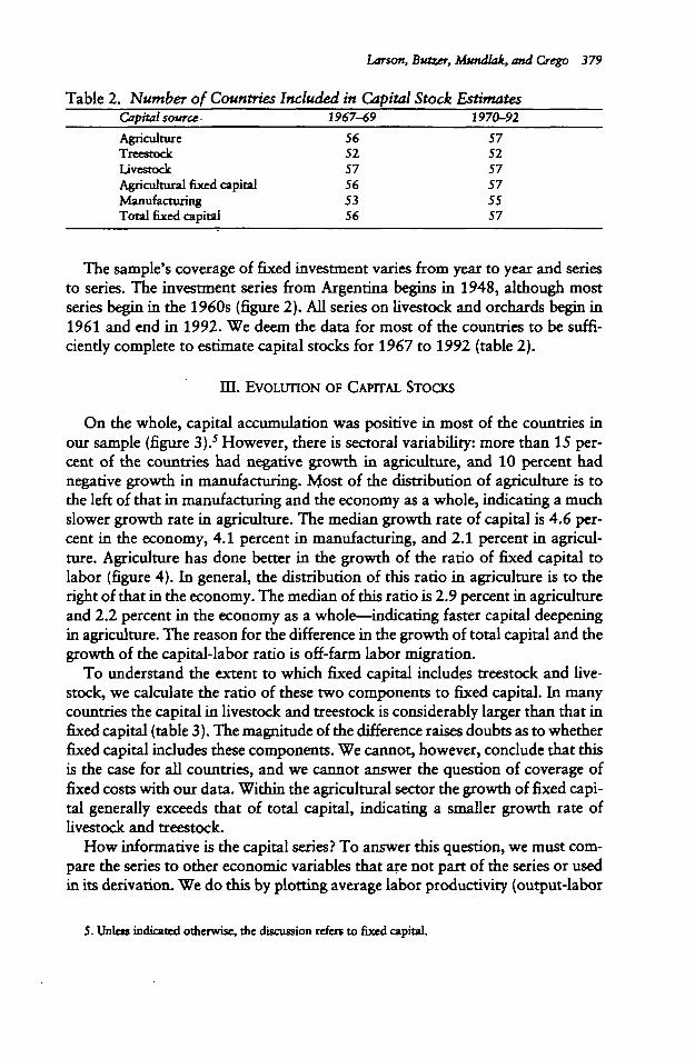
Table 2. Number of Countries Included in Capital Stock EstimatesCapital source -
AgricultureTreestockLivestockAgricultural fixed capitalManufacturingTotal fixed capital
1967-69
565257565356
1970-92575257575557
The sample's coverage of fixed investment varies from year to year and seriesto series. The investment series from Argentina begins in 1948, although mostseries begin in the 1960s (figure 2). All series on livestock and orchards begin in1961 and end in 1992. We deem the data for most of the countries to be suffi-ciently complete to estimate capital stocks for 1967 to 1992 (table 2).
m. EVOLUTION OF CAPITAL STOCKS
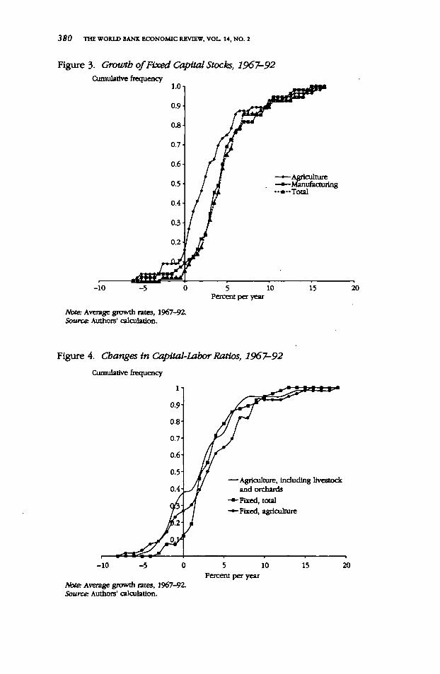
On the whole, capital accumulation was positive in most of the countries inour sample (figure 3).J However, there is sectoral variability: more than 15 per-cent of the countries had negative growth in agriculture, and 10 percent hadnegative growth in manufacturing. Most of the distribution of agriculture is tothe left of that in manufacturing and the economy as a whole, indicating a muchslower growth rate in agriculture. The median growth rate of capital is 4.6 per-cent in the economy, 4.1 percent in manufacturing, and 2.1 percent in agricul-ture. Agriculture has done better in the growth of the ratio of fixed capital tolabor (figure 4). In general, the distribution of this ratio in agriculture is to theright of that in the economy. The median of this ratio is 2.9 percent in agricultureand 2.2 percent in the economy as a whole—indicating faster capital deepeningin agriculture. The reason for the difference in the growth of total capital and thegrowth of the capital-labor ratio is off-farm labor migration.
To understand the extent to which fixed capital includes treestock and live-stock, we calculate the ratio of these two components to fixed capital. In manycountries the capital in livestock and treestock is considerably larger than that infixed capital (table 3). The magnitude of the difference raises doubts as to whetherfixed capital includes these components. We cannot, however, conclude that thisis the case for all countries, and we cannot answer the question of coverage offixed costs with our data. Within the agricultural sector the growth of fixed capi-tal generally exceeds that of total capital, indicating a smaller growth rate oflivestock and treestock.
How informative is the capital series? To answer this question, we must com-pare the series to other economic variables that are not part of the series or usedin its derivation. We do this by plotting average labor productivity (output-labor
5. Unless indicated otherwise, the discussion refers to fixed capital.
3 80 THE WORLD BANK ECONOMIC REVIEW, VOL. 14, NO. 2
Figure 3. Growth of Fixed Capital Stocks, 1967-92Cumulative frequency
•AgricultureManufacturingTotal
-10
Note: Average growth rates, 1967-92.Source-Authors' calculation.
5 10Percent per year
15 20
Figure 4. Changes in Capital-Labor Ratios, 1967-92
-10
Note: Average growth rates, 1967-92.Source: Authors' calculation.
—Agriculture, including livestockand orchards
•*- Fixed, total-•-Fixed, agriculture
5 10Percent per year
15 20
Larson, Butzer, Mundlak, and Crego 381
Table 3. Ratio of Treestock(averages over 1967-92)Country
ratio) against the capital-labor ratio for the economy as a whole and for agricul-ture (figures 5 and 6). These scatter diagrams trace the production function interms of capital intensity, without allowing for the effects of other pertinent vari-ables. Nevertheless, it is dear that the capital series is informative and relevant. Amore detailed analysis of the production function using these data appears inMundlak, Larson, and Butzer (1999). These data are used also in Martin andMitra (1999) and Mundlak, Larson, and Crego (1998).
IV. SENSITIVITY ANALYSIS
We have used a fairly elaborate method to calculate the change in productivityor, simply, depreciation (see appendix B for a discussion of depreciation). Twoquestions arise in this connection. First, how sensitive is the result to the choiceof parameters? And, second, how much is gained by using this method rather
382 THE WORLD »ANX ECONOMIC REVIEW, VOL. 14, NO. 2
Figure 5. Economywide Output per Worker and Capital per Worker, 1967-92
Note: Capital includes livestock and treestock.Source: Capital- Authors' calculations; Labor International Labor Organization; GDP: World Bank, United
Nations, OECD, IMF, and various country sources.
Larson, Butzer, Mundiak, and Crego 383
than simpler conventional methods? We answer the two questions by comparingour results above with those obtained using a different set of parameters.
In what follows we label as the base calculation the results derived above,which we obtained using the parameter values in table 1. We report the meanratios of alternative computations of the fixed capital stock for the years 1970,1980, and 1990 relative to the base calculation (table 4). The results reported inthe first five columns of table 4 were obtained using the same parameters as thebase calculation except for the changes that appear in the column heading. Theresults range from 0.59 with P = -1 to 1.37 with P = 1, indicating that the loweris the initial depreciation (the higher is the value of P), the higher is the level ofcapital stock. When p is higher, the capital stock is larger because investmentsare more productive in their old age.
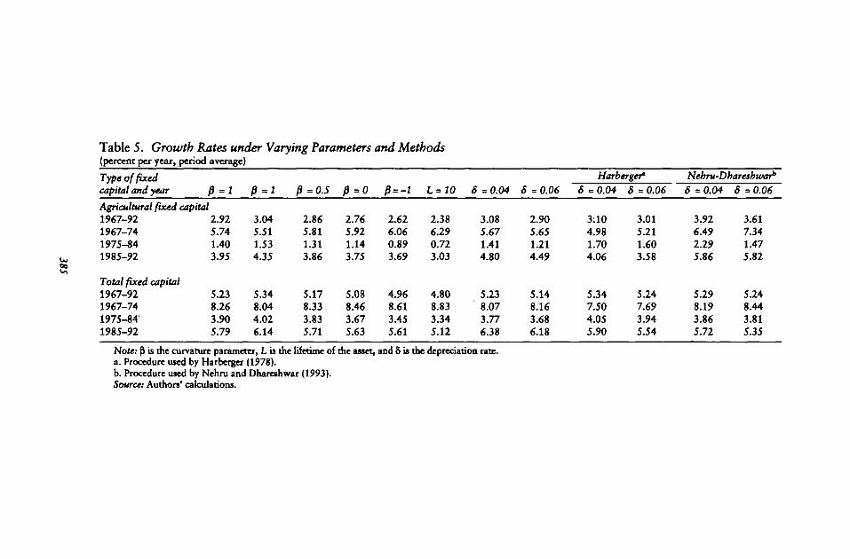
The choice of parameters affects the level of the capital stock, but it only slightlyaffects the growth rate of the capital stock (table 5).6 Essentially, the growth rateof the capital stock is determined largely by the investment rate. We can see thisfrom the low growth rates in 1975-84 relative to the other two subperiods. Thisdifference is sizable, and it is detected by each of the alternative calculations.Another indication is the sensitivity of the growth rate to the lifetime of the in-vestment. Reducing the lifetime mean from 20 to 10 years (keeping the coeffi-cient of variation constant) makes the capital stock more sensitive to fluctuationsin investment.
Why does the choice of parameters affect the level but not the growth rate ofcapital? This outcome is related to the level of disaggregation of capital goods,the time profile of their productivity, and the changes in their composition. Whenthere are several components of capital with different time profiles, a change inthe composition of investment will affect the growth rate of capital in addition tothe level. We do not detect this in our calculations because data limitations pre-vent us from decomposing fixed investment into its components.
Do we gain by refining the method of computing the productivity coefficient?To answer this, we assume geometric depreciation, then calculate the capitalstock by varying only one parameter, the depreciation rate, 8, so that st•. = (1 - tyfor / = 0 , . . . , t - T. We present results for two alternative values of 8, 0.04 and0.06 (tables 4 and 5). The value of 0.06 produces capital levels and growth ratesthat come close to the values obtained in our base calculation.
We also examine the sensitivity of the results to the choice of the initial valueof capital. We consider two alternatives described in Nehru and Dhareshwar(1993). The first is the procedure used by Harberger (1978), which is based onthe assumption of a constant capital-output ratio. This procedure leads to thefollowing equation:
(5) KM =/,/{* +8)
6. We calculate the growth rates using ordinary least squares regressions of the log of capital on time.
Table 4. Comparison of Series Means Calculated Using Varying Methods for 1970, 1980, and 1990Type of fixedcapital and year
Agricultural fixed capital197019801990
1.341.311.37
Total fixed capital
197019801990
1.281.261.31
p =o.s
0.910.910.90
0.920.920.91
p=o
0.770.770.74
0.780.790.76
p = -l
0.620.620.59
0.640.650.61
L = 10
0.580.600.53
0.620.640.58
8 =0.04
1.521.511.61
1.221.181.22
8 = 0.06
1.111.091.11
0.990.970.98
Harberger*
8 =0.04
1.411.291.34
1.131.141.19
8 = 0.06
0.990.991.00
0.930.950.96
Nehru-Dhareshtvarh
8 =0.04
1.211.261.44
1.271.181.24
8 = 0.06
0.940.991.10
0.990.961.00
Note: B is the curvature parameter, L is the lifetime of the asset, and 8 is the depreciation rate.a. Procedure used by Harberger (1978).b. Procedure used by Nehru and Dhareshwar (1993).Source: Authors' calculations.
Table 5. Growth Rates under Varying Parameters and Methods(percent per year, period average)
Ui00
Type of fixedcapital and year P=lAgricultural fixed capital1967-921967-741975-841985-92
Total fixed capital1967-921967-741975-841985-92
2.925.741.403.95
5.238.263.905.79
p=l
3.045.511.534.35
5.348.044.026.14
P =0.5
2.865.811.313.86
5.178.333.835.71
P =0
2.765.921.143.75
5.088.463.675.63
P = -l
2.626.060.893.69
4.968.613.455.61
1 = 10
2.386.290.723.03
4.808.833.345.12
S =0.04
3.085.671.414.80
5.238.073.776.38
S = 0.06
2.905.651.214.49
5.148.163.686.18
Harberger*5 =0.04
3:104.981.704.06
5.347.504.055.90
S = 0.06
3.015.211.603.58
5.247.693.945.54
Nehru-Dhareshwarb
S =0.04
3.926.492.295.86
5.298.193.865.72
S => 0.06
3.617.341.475.82
5.248.443.815.35
Note: P is the curvature parameter, L is the lifetime of the asset, and 8 is the depreciation rate.a. Procedure used by Harberger (1978).b. Procedure used by Nehru and Dhareshwar (1993).Source: Authors' calculations.
386 THE WORLD BANK ECONOMIC REVIEW, VOL. 14, NO. 2
where g is the growth rate of output. Harberger uses three-year averages of thegrowth rate of output and investment to reduce the effects of short-term varia-tions. Applying this method to our data shows that the results with 8 = 0.06 aresimilar to our initial results.
The second procedure is a modification of the Harberger approach proposedby Nehru and Dhareshwar. Rather than use three-year averages of investment toestimate the initial stock of capital, the initial level of investment is fitted using aregression of the log of investment on time. Thus the estimation is less sensitiveto initial-period conditions. The investment series used in the regression was trun-cated in 1973. The results do not differ much from those derived using the Har-berger approach.
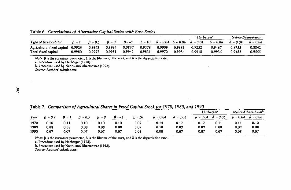
The correlation between the capital stock obtained with the alternative calcu-lations and our results is high for most of the series (table 6). The correlation isparticularly strong for the choice of curvature parameters. Consistent with theresults of tables 4 and 5, although the choice of parameters and aggregation andseeding techniques may affect the levels of capital stock, they do not seem toaffect the movements of the capital stock. However, the correlation is affected bythe choice of the initial value of capital used in the integration. Obviously, thecorrelations are lower for the Nehru-Dhareshwar calculations than for ours, sinceour calculations are based on more information.
Finally, alternative calculations of the share of agriculture in fixed capital forthe sample as a whole show that the share declines over the years, from 10 per-cent in 1970 to 7 percent in 1990 (table 7). The figures vary somewhat with themethod, reflecting the variations observed in table 4. Differences between theseries tend to remain the same across time. Consequently, the growth rates of thecapital stock vary more by subperiod than by choice of method or parameter.
V. CONCLUSION
This article reports a new time series on investment data for agriculture, manu-facturing, and the economy as a whole. A common method is applied to deriveestimates of sector-level capital stocks for 62 countries during 1967-92. Thedatabase fills a long-standing need for a sectoral measure of one of the basiccomponents of economic production and a key determinant of growth.
The capital stocks for agriculture and the economy as a whole consist of threecomponents—fixed capital, livestock, and orchards—whereas that of manufac-turing consists of fixed capital alone. Integrating fixed investment to capital stocksrequires that we select the depreciation rate and the initial value of the series. Thechoice of the depreciation rate is based on an aging pattern determined by acurvature parameter and the lifetime of the asset. Simulations using our datashow that the level of the capital stock is sensitive to the choice of parameters.However, the growth rate of the stock is fairly robust to the choice of the curva-ture parameter and somewhat sensitive to the assumed lifetime. The results aremore sensitive to the choice of the initial value of the series. We suggest a proce-
Uloo
Table 6. Correlations of Alternative Capital Series with Base Series
Type of fixed capitalAgricultural fixed capitalTotal fixed capital
p=l0.99230.9980
P =0.50.99730.9997
p=o0.99340.9981
P = -l0.98370.9942
L = 100.95760.9831
S =0.040.99090.9970
8 m 0.060.99620.9986
Harberger'8 =0.040.92320.9918
8 = 0.060.94670.9936
Nehru-Dhareshwarh
8 e 0.04 8 = 0.060.8753 0.88420.9482 0.9555
Note: P is the curvature parameter, L is tbe lifetime of the asset, and S is the depreciation rate.a. Procedure used by Harberger (1978).b. Procedure used by Nehru and Dhareshwar (1993).Source: Authors' calculations.
Table 7. Comparison of Agricultural Shares in Fixed Capital Stock for 1970,1980, and 1990
Year
197019801990
P =0.7
0.100.080.07
P=l0.110.080.07
P =0.5
0.100.080.07
p °o0.100.080.07
p = -l
0.100.080.07
L = 10
0.090.070.06
8 =0.040.140.100.08
8 = 0.06
0.120.090.07
Harberger'8 =0.04
0.120.090.07
8 = 0.060.110.080.07
Nehru-Dhareshwarb
8 =0.04
0.110.090.08
8 =0.06
0.100.080.07
Note: P is the curvature parameter, L is the lifetime of the asset, and S is the depreciation rate.a. Procedure used by Harberger (1978).b. Procedure used by Nehru and Dhareshwar (1993).Source: Authors' calculations.
388 THE WORLD BANK ECONOMIC REVKW, VOL. 14, NO. 2
dure for determining the initial value that uses country-specific investment rates.The robustness of the growth rate to the curvature parameters may disappearwhen the investment data become available at a lower level of aggregation.
There is a caveat and a note of hope regarding this effort. The definition offixed investment, as well as the definitions of agriculture and manufacturing,may differ from country to country and possibly within countries over time. Inaddition, reporting errors are Likely to arise, and these may affect cross-countrycomparisons. On the positive side, we obtained our data through an intensivelibrary search of country publications. Nevertheless, we suspect that the scopefor such a search has not been exhausted and, specifically, that census data andother national sources might be found and used to augment country and timecoverage. We hope that further research will extend and improve on our initialwork.
Collectively, the data suggest that as economies grow, capital stocks accumu-late, and the composition of capital changes. Together and individually, capitalstocks in agriculture and manufacturing constitute a smaller share of the totalcapital stock than they did 20 years ago. Agriculture has become more capitalintensive in most countries, even though agricultural capital stocks—includinglivestock and orchards—have declined in about 30 percent of the countries. Thecomposition of agricultural capital has also changed in most countries. Capitalfrom fixed investments in machinery, irrigation, and buildings has become in-creasingly important, while capital of agricultural origin, such as livestock andtreestock, has declined in importance.
APPENDIX A. CONVERSION AND DEFLATION
The real exchange rate used in equation 4 is obtained with price indexes, p*and ptt which measure prices of different baskets of goods in each country. Analternative measure is the exchange rate based on purchasing power parity (PPP).
The PPP gives the dollar value of an identical—quality-adjusted—output basketin different countries. Under the theory of the law of one price this exchange rate,ep, should equal the local price of the basket divided by the foreign price. Thenthe exchange rate will always adjust to compensate for changes in domestic andworld prices, and ep will equal 1. Under this assumption ep should be less volatilethan e.
The Penn World Tables present the dollar price of identical output baskets fora large number of countries, facilitating the derivation of ep. We compute thecorrelation coefficient between ep and e. For most countries this correlation ishigh, although it falls during periods of high price volatility. The empirical litera-ture on the PPP is not supportive in that there are considerable deviations from 1in the short run; still, the theory is thought to be useful in describing long-termtrends. There are several basic reasons why ep deviates from 1. The law of oneprice covers the relationship between domestic and foreign prices only for trad-able goods, whereas the price of any good has a nontradable component. Also,
Larson, Butzer, Mundlak, and Crego 389
the law does not take tariffs into account. The first problem does not apply toe because the domestic price index is an aggregate of the prices of tradableand nontradable goods, which are assigned the specific weights of the country inquestion.
To interpret equation 4, substitute the definition of e into the equation toobtain K* m p,Kt/Etp *, where the numerator is the nominal value of fixed capital.The procedure amounts to converting capital to nominal dollar values using nomi-nal exchange rates and then deflating by an index of the world price. Martin andMitra (1999), using our fixed capital series, convert the values using a constantexchange rate, £ 0 (say, the base year):
(A-l)
The relationship between this measure and ours is given by
(A-2) (Kt)/(AKV = Eo/e,.
Thus if the nominal exchange rate changed only at the rate of the ratio ofdomestic to world prices, the two measures would be identical. Otherwise, it isquestionable that subscribing to a constant exchange rate is preferable to usingthe real exchange rate for conversion. If the pertinent exchange rate were con-stant, then ep would equal 1, but this is not the case.
APPENDIX B. DEPRECIATION
Depreciation plays an explicit role only in the sensitivity analysis, in which wecompare our measure to alternatives. It is therefore useful to review the role ofdepreciation in our estimates. In the case of fixed capital the total depreciation inyear t of an asset of age / is the decline in productivity, 1-5/, and the averageannual rate is the total divided by /. In practice this decline is determined bychoosing a rule and a set of parameters. We choose a rule based on the averagelife expectancy of the asset (L) and a curvature parameter (P). As already noted,this gives rise to a concave productivity curve for positive values of p. A morecommon approach is to assume that depreciation is geometric at rate 8, in whichcase 5, = (1 - 5y for ; = 0, ... , t - T, and the perpetual inventory yields Kt =(1 - b)Kt_1 + Io generating a convex productivity curve.
The present value of capital is forward-looking and only partially based on physi-cal productivity. It is determined by the physical productivity of the asset, the ex-pected price of output and inputs at each point in time for the remaining life, thediscount factor, and the asset's remaining years of service. Thus value depreciationdiffers from physical depreciation. To examine value depreciation, assume thatexpected prices are constant, and thus the time path of value depends on the de-cline in future performance due to the passage of time and the expected length ofremaining life. For example, assume that an asset has a life of length L and pro-
390 THE WORLD BANK ECONOMIC REVIEW, VOL 14, NO. 2
Figure B-l. Value of Capital Assets
Remaining asset value
Tune in use
duces x dollars a year. If we ignore discounting, the value of the asset depreciatesby x dollars with each year of use, and after ; years of use the value is (L - j)xdollars. This value falls linearly with time along the line segment AL in figure B-l.When we also discount the future returns from the asset, the value path changes tothe path ABCL, which falls below the path AL of the undiscounted value. Depre-ciation along ABCL reflects the decline in discounted future returns. Consequently,ABCL can be convex even when the productivity path is not.
To trace the behavior of the asset's value over time, let the discount rate be aL-
and the value of capital at the end of period 0 be equal to Vo = V a'x,. Tosimplify, assume x, = x for all i and write: 1=1
(B-l)Vo = ax + a2x + ... + aLx
3 ax + a?x + V2
where V;- is the value, taken at period 0, of the income stream after; periods of useor simply of an asset of age /. We can draw the value pam to trace V;- as a function of/ (the time use of the asset). For nontrivial discounting (a < 1) we obtain Vi-V2<Vo - Vj so that the value path is convex, as illustrated by the curve ABCL. In theextreme case of no discounting, a = 1 and the path follows a straight line. This is anupper bound for the value curve, implying that, unlike the productivity path, itcannot be strictly concave. By implication, geometric depreciation functions relatebetter to value measures of capital than physical measures.
Larson, Butzer, Mundlak, and Crego 391
In the case of treestock we evaluate the stock at midlife, and depreciation doesnot appear explicitly. However, our procedure captures any technical changethat affects the yield of the orchard through our computation of revenue. In thecase of livestock the only depreciation under consideration are discards, whichare handled through changes in inventory.
REFERENCES
The word "processed" describes informally reproduced works that may not be com-monly available through library systems.
Akiyama, Takamasa, and Pravin Trivedi. 1987. "Vintage Production Approach to Peren-nial Crop Supply: An Application to Tea in Major Producing Countries." Journal ofEconometrics 36(1):133-61.
Ball, V. Eldon, Jean-Christophe Bureau, Jean-Pierre Butault, and Heinz Peter Witzke.1993. "The Stock of Capital in European Community Agriculture." European Reviewof Agricultural Economics 20:437-50.
Crego, Al, Donald Larson, Rita Butzer, and Yair Mundlak. 1998. "A New Database onInvestment and Capital for Agriculture and Manufacturing." Policy Research Work-ing Paper 2013. DRG, World Bank, Washington, D.C. Processed.
Griliches, Zvi. 1963. "Capital Stock in Investment Function: Some Problems of Conceptand Measurement." In Carl F. Christ, ed., Measurement in Economics. Stanford, Calif.:Stanford University Press.
Harberger, Arthur. 1978. "Perspectives on Capital and Technology in Less DevelopedCountries." In M. J. Arris and A. R. Nobay, eds., Contemporary Economic Analysis.London: Croom Helm.
Hulten, C. R. 1990. "The Measurement of Capital." In Ernst R. Berndt and Jack E.Triplett, eds., Fifty Years of Economic Measurement. Chicago: University of ChicagoPress.
International Monetary Fund. 1998. International Financial Statistics. Washington, D.C.Martin, Will, and Devashish Mitxa. 1999. "Productivity Growth and Convergence in
Agriculture and Manufacturing." Policy Research Working Paper 2171. DRG, WorldBank, Washington, D.C. Processed.
Mundlak, Yair, Donald F. Larson, and Rita Butzer. 1999. "Rethinking within and be-tween Regressions: The Case of Agricultural Production Functions." Annalesd'Economie et Statistique 55-56:475-501.
Mundlak, Yair, Donald F. Larson, and Al Crego. 1998. "Agricultural Development: Is-sues, Evidence, and Consequences." In Yair Mundlak, Michael Bruno, and DanielCohen, eds., Contemporary Economic Issues: Proceedings of the Eleventh World Con-gress of the International Economic Association, Tunis: Labour, Food, and Poverty.New York: St, Martin's Press.
Nehru, Vikram, and Ashok Dhareshwar. 1993. "A New Database on Physical CapitalStock: Sources, Methodology, and Results." Revista de Andlisis Economico 8(1):37-59.
United Nations. 1991. National Accounts Statistics: Main Aggregates and Detailed Tables.New York.