A deformation based blank design method for formed parts

W. Hammami • R. Padmanabhan • M. C. Oliveira •

H. BelHadjSalah • J. L. Alves • L. F. Menezes

Received: 18 November 2008 / Accepted: 11 September 2009 / Published online: 23 October 2009

� Springer Science+Business Media, B.V. 2009

Abstract Blank design is an important task in sheet

metal forming process optimization. The initial blank

shape has direct effect on the part quality. This paper

presents a deformation based blank design approach to

determine the initial blank shape for a formed part. The

blank design approach is integrated separately into

ABAQUS, and DD3IMP, a research purpose in-house

FEA code, to demonstrate its compatibility with any

FEA code. The algorithm uses FE results to optimize

the blank shape for a part. Deep drawing simulation of a

rectangular cup geometry was carried out with an

initial blank shape determined empirically. The blank

shape was iteratively modified, based on the deforma-

tion history, until an optimal blank shape for the part is

achieved. The optimal blank shapes predicted by the

algorithm using both FEA softwares were similar.

Marginal differences in the shape error indicate that the

deformation history based push/pull technique can

effectively determine an optimal blank shape for a part

with any FEA software. For the shape error selected,

both procedures estimate the optimal blank shape for

the part within five iterations.

Keywords Blank shape optimization �Deep drawing � FE simulation � Push/pull technique

Abbreviations

DD3IMP Contraction of deep-drawing 3D

IMPlicit code

DD3SHAPE Contraction of deep-drawing 3D

blank SHAPE optimization code

DD3TRIM Contraction of deep-drawing 3D

TRIMming code

IGES Initial graphics exchange

specification

NURBS Non uniform rational basis spline

1 Introduction

Initial blank shape is one of the important process

parameters in sheet metal forming that determines the

W. Hammami � H. BelHadjSalah

Laboratoire de Genie Mecanique, Ecole d’Ingenieurs

de Monastir, Monastir, Tunisie

e-mail: Walid.Hammami@ulg.ac.be

H. BelHadjSalah

e-mail: hedi.belhadjsalah@enim.rnu.tn

R. Padmanabhan (&) � M. C. Oliveira � L. F. Menezes

CEMUC, Centre of Mechanical Engineering

of the University of Coimbra, Polo II, Coimbra, Portugal

e-mail: padmanabhan@dem.uc.pt

M. C. Oliveira

e-mail: marta.oliveira@dem.uc.pt

L. F. Menezes

e-mail: luis.menezes@dem.uc.pt

J. L. Alves

Department of Mechanical Engineering, University

of Minho, Campus de Azurem, Guimaraes, Portugal

e-mail: jlalves@dem.uminho.pt

123

Int J Mech Mater Des (2009) 5:303–314

DOI 10.1007/s10999-009-9103-9

quality and final cost of the formed part. An optimal

blank contributes to minimize forming defects such

as wrinkling and tearing resulting in a good quality

part. Many blank design approaches have been

proposed to determine the optimum initial blank

shape. A slip line field theory based method to

determine optimum blank shape was described by

Kuwabara and Si (1997). The method is capable of

predicting an optimal blank shape within few seconds

but assumes the blank material as isotropic, rigid-

perfectly plastic and does not deform, i.e., the

thickness of the blank does not change during the

deep drawing operation. A finite element method

based inverse approach to determine optimum blank

contour for industrial parts was described by Guo

et al. (2000). The approach uses the knowledge of

discretized 3D shape of the final part. The efficiency

and convergence rate is dependant on the assumed

initial blank. A roll-back method to predict optimum

blank shapes for industrial parts was proposed by

Kim et al. (2000). The deformed blank shape is

compared with the target shape and necessary

modification is carried out in the initial blank. The

optimal blank shape for a part was obtained by Park

et al. (1999) using a deformation path iteration

method. In all these approaches, either the finite

element mesh size was altered during the optimiza-

tion procedure or only the part’s flange area was

considered. In this study, a blank design method

based on the deformation behavior of the blank is

presented. The blank design method using a push/pull

technique, described in more detail in (Padmanabhan

et al. 2009), is integrated with two finite element

analysis codes, namely ABAQUS (Version 6.4) and

DD3IMP (Menezes and Teodosiu 2000), in order to

evaluate the efficiency of the method applied with

different simulation tools. The procedure includes

deep drawing simulations integrated with the push/

pull optimization technique, which is integrated with

both codes using B-spline curve or NURBS surface

interpolation, for ABAQUS and DD3IMP, respec-

tively. The combined numerical tools are tested to

prove that it can be an economical solution in

reducing time and material. In order to achieve an

integrated optimization procedure, the programming

language PYTHON is used to apply the push/pull

technique and to input the changes in geometry in

ABAQUS. In DD3IMP the changes in geometry are

introduced using DD3TRIM, an in-house code used

to trim 3D solid finite meshes (Baptista et al. 2006).

Following sections describe the push/pull optimiza-

tion technique, integration of this technique with

ABAQUS and DD3IMP and, finally, its application

to a rectangular cup example.

2 Blank shape optimization procedure

The blank shape optimization procedure involves an

important task of modifying the blank contour based

on the deformation behaviour and the required target

shape. A push/pull technique is used in this study to

modify the blank shape as described below.

2.1 Push/pull technique

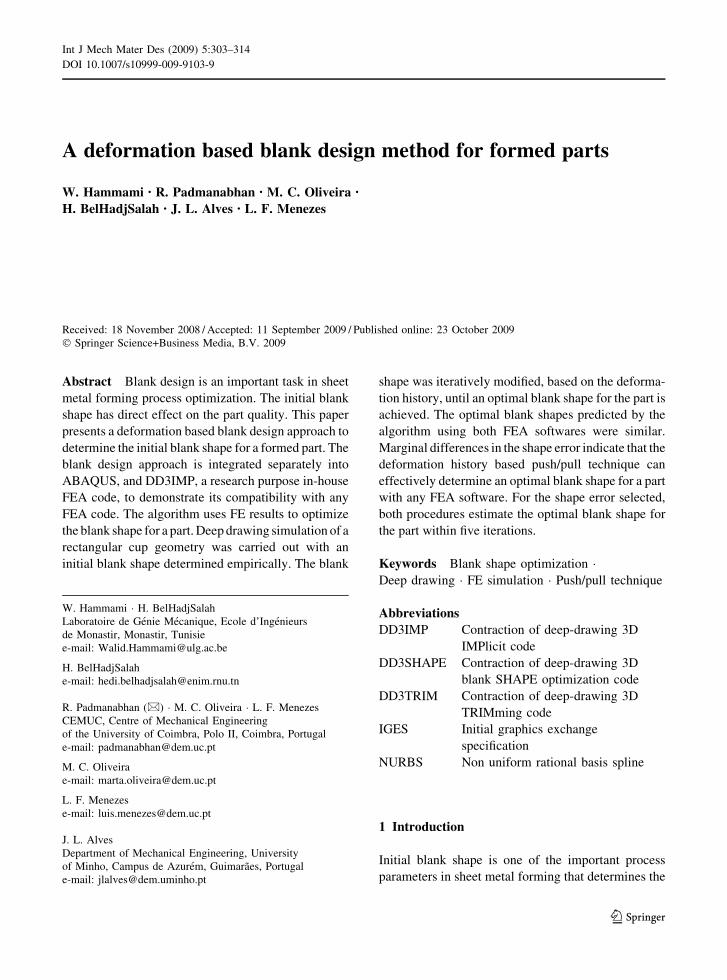
Consider a blank, with an initial contour indicated by

dashed line in Fig. 1, subjected to deep drawing.

Depending on the part geometry and the non-linear

flow of the blank during the forming process, the

contour at the end of process may take a shape

different from the required contour. In Fig. 1, the

final contour is shown by the continuous line, against

the required contour indicated by the thick line. The

set of points P1; P2; P3; . . .;Pnð Þ; defining the

original surface with positions Xinit; may lie either

inside or outside or on the target contour after deep

drawing; with their positions defined by Xfinal. The

intersection of their trajectory and the target contour

defines Xinter, as shown in the figure.

As illustrated in the figure, the final position of

point P1 is located inside the target contour, hence,

the point in the new surface has to move outside the

initial surface. On contrary, since the final position of

point P2 is located outside the target contour, the

point in the new surface has to move inside the initial

surface. Point P3 does not need correction as it lies on

the target contour. The knowledge of the initial

position Xinit; the final position Xfinal; and the

intersection position Xinter enables the push/pull

technique to calculate the positions of the new set

of points using,

P�i ¼ Xiniti þ Xinter

i � Xfinali

� �; with i ¼ 1; . . .; n;

ð1ÞAssuming a linear trajectory for material flow

during deep drawing, the vector Xinteri � Xfinal

i defines

the direction and the distance to move each of the initial

304 W. Hammami et al.

123

points selected. n is the number of points considered

along the blank contour for the push/pull technique.

This push/pull technique, if applied with a damping

coefficient n, controls the oscillations around the target

contour that may occur due to the iterative procedure

adopted. Therefore Eq. 1 can be written as

P�i ¼Xiniti þ n Xinter

i �Xfinali

� �; with i¼ 1; . . .;n: ð2Þ

The objective of the optimization algorithm is to

identify the difference between the existing flange

contour and the required target contour and provide a

corrective solution that minimizes the difference. In

order to guarantee the convergence of the iterative

procedure it is important that the initial process

parameters like, the tools geometry, the mechanical

properties of the blank, the friction conditions and the

blank holder force are fixed in the numerical simulation

model, during the optimization procedure. An initial

blank shape is normally determined based on empirical

formulae.

The optimization algorithm used in this study uses a

geometric measure called geometrical shape error

(GSE), to quantify the deviation between the flange and

the target contours. This error, expressed in the same

dimensions used for the point coordinates, is defined as

the root mean square of the shape difference between

the target shape and the deformed shape as in the

following equation, proposed by Park et al. (1999):

GSE ¼ffiffiffiffiffiffiffiffiffiffiffiffiffiffiffiffiffiffiffiffiffiffiffiffiffiffiffiffiffiffiffiffiffiffiffiffiffiffiffiffiffiXn

i¼1

1

nXinter

i � Xfinali

�� ��2

s

: ð3Þ

The vector norm used corresponds to the Euclidean.

The geometrical shape error defines the stopping

criterion for the blank shape optimization procedure.

When the GSE reaches a value less than a predeter-

mined value d for the required accuracy in the flange

shape, the iterative procedure is stopped because the

optimal blank shape for the part has been obtained.

For the example presented in this work, the error in

the flange shape (d) less than 0.5 mm is used as the

stopping criterion.

The GSE allows correct estimation of the distance

between the actual flange contour and the target

contour. However, by definition it is not possible with

the GSE to evaluate whether the actual flange contour

is inside or outside the target contour. To clearly

understand the shape error, a measure called target

shape error (TSE) is used to quantify the magnitude

of deviation of the flange contour from the required

target contour. The TSE, expressed in the same

dimensions used for point coordinates, is defined as:

TSE¼ 1

n

Xn

i¼1

sign 1�Xinit

i �Xfinali

�� ��

Xiniti �Xinter

i

�� ��

!

Xiniti �Xfinal

i

�� ��" #

ð4Þ

where the sign function is used to identify whether a

point is inside or outside the target contour. The

target shape error is used mainly to analyze the

convergence rate towards the solution, since it allows

detecting oscillations around the target contour.

2.2 Implementation of push/pull technique

with FEM simulations

2.2.1 ABAQUS

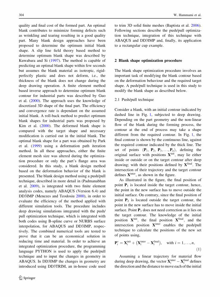
The contour of the initial blank is defined using a

three degree B-spline curve, which is divided by a set

of n control points, as presented in Fig. 2. The n

Fig. 1 Push/pull technique

used to adjust flange

contour

A deformation based blank design method 305

123

control points are selected for the initial blank shape,

normally deduced empirically. These points are used

to divide the blank surface along n-1 radial segments,

defined by the ri; i ¼ 1; . . .; n� 1 radial directions.

The use of these control points allows changing the

shape of the blank contour, in each iteration, and

automatically producing the mesh for the new blank.

The coordinates of the n control points are changed,

in each iteration, applying the push/pull technique

explained previously and implemented in ABAQUS

through PYTHON. This procedure alters each parti-

tion line ri; i ¼ 1; n� 1 rendering the new blank

geometry. The new coordinates of each control point,

determined using the push/pull technique are input to

ABAQUS. ABAQUS updates the three degree B-

spline curve automatically, based on the control

points defined. The outer boundary of the blank

geometry is described by the B-spline curve (see

Fig. 2). The definition of the B-spline curve allows

automatic meshing of the blank surfaces. The result-

ing mesh is subjected to deep drawing simulation in

ABAQUS FEA code. The flange contour of the

formed part is compared with the required target

contour. If the flange contour is different from target

contour, the initial B-spline is corrected and a new set

of n - 1 surfaces are produced. These new surfaces

are used to produce intermediate blank shape with a

new mesh, which is subjected to deep drawing

process. The application of the push/pull technique

to the surfaces based on B-spline allows guaranteeing

a smooth blank contour, in each iteration.

The programming language PYTHON is used to

input the data into ABAQUS, leading to an automatic

blank shape optimization procedure implemented

with the commercial software. The blank shape

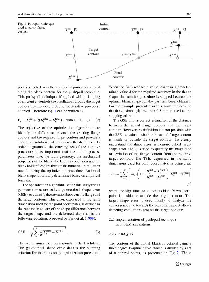
optimization procedure is illustrated in Fig. 3.

As illustrated in Fig. 3, this procedure is repeated

until the deviation between flange contour and target

contour falls below the user defined value, d. The

optimization procedure is fully automated due to the

combination of ABAQUS and PYTHON.

2.2.2 DD3IMP

Three numerical tools, DD3IMP, DD3TRIM and

DD3SHAPE are used in this procedure to determine

the optimal blank shape for a part. Deep drawing

simulations were carried out using the in-house finite

element code DD3IMP. DD3IMP is specifically

developed to simulate sheet metal forming processes.

The evolution of the deformation process is described

by an updated Lagrangian scheme. A fully implicit

algorithm is used to guarantee the satisfactory

equilibrium of the deformable body, in each incre-

ment, as described by Menezes and Teodosiu (2000).

In sheet metal forming processes, the boundary

conditions are dictated by the contact established

between the blank sheet and tools. Such boundary

conditions are continuously changing during the

forming process, increasing the importance of a

correct evaluation of the actual contact surface and

the kind of contact that is established in each point of

the deformable body. A master–slave algorithm is

adopted, with the tools behaving as rigid bodies. The

Coulomb’s classical law models the friction contact

problem between the rigid bodies (tools) and the

deformable body (blank sheet). The problem of the

contact with friction is treated by an augmented

Lagrangian approach. The abovementioned fully

implicit Newton–Raphson scheme is used to solve,

Fig. 2 Model used to implement the push/pull technique in

ABAQUS

Fig. 3 Blank shape optimization procedure in ABAQUS

306 W. Hammami et al.

123

in a single loop, all the problem non-linearities

associated to the problem of contact with friction and

the elasto-plastic behavior of the deformable body.

Further details about the numerical strategies adopted

in DD3IMP can be obtained from the work of

Oliveira et al. (2008).

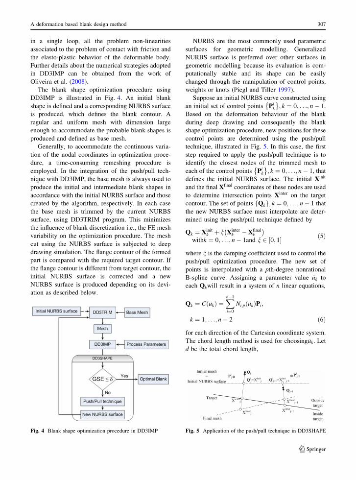
The blank shape optimization procedure using

DD3IMP is illustrated in Fig. 4. An initial blank

shape is defined and a corresponding NURBS surface

is produced, which defines the blank contour. A

regular and uniform mesh with dimension large

enough to accommodate the probable blank shapes is

produced and defined as base mesh.

Generally, to accommodate the continuous varia-

tion of the nodal coordinates in optimization proce-

dure, a time-consuming remeshing procedure is

employed. In the integration of the push/pull tech-

nique with DD3IMP, the base mesh is always used to

produce the initial and intermediate blank shapes in

accordance with the initial NURBS surface and those

created by the algorithm, respectively. In each case

the base mesh is trimmed by the current NURBS

surface, using DD3TRIM program. This minimizes

the influence of blank discretization i.e., the FE mesh

variability on the optimization procedure. The mesh

cut using the NURBS surface is subjected to deep

drawing simulation. The flange contour of the formed

part is compared with the required target contour. If

the flange contour is different from target contour, the

initial NURBS surface is corrected and a new

NURBS surface is produced depending on its devi-

ation as described below.

NURBS are the most commonly used parametric

surfaces for geometric modelling. Generalized

NURBS surface is preferred over other surfaces in

geometric modelling because its evaluation is com-

putationally stable and its shape can be easily

changed through the manipulation of control points,

weights or knots (Piegl and Tiller 1997).

Suppose an initial NURBS curve constructed using

an initial set of control points Pik

� �; k ¼ 0; . . .; n� 1.

Based on the deformation behaviour of the blank

during deep drawing and consequently the blank

shape optimization procedure, new positions for these

control points are determined using the push/pull

technique, illustrated in Fig. 5. In this case, the first

step required to apply the push/pull technique is to

identify the closest nodes of the trimmed mesh to

each of the control points Pik

� �; k ¼ 0; . . .; n� 1, that

defines the initial NURBS surface. The initial Xinit

and the final Xfinal coordinates of these nodes are used

to determine intersection points Xinter on the target

contour. The set of points Qkf g; k ¼ 0; . . .; n� 1 that

the new NURBS surface must interpolate are deter-

mined using the push/pull technique defined by

Qk ¼ Xinitk þ n Xinter

k � Xfinalk

� �

withk ¼ 0; . . .; n� 1and n 2 0; 1½ � ð5Þ

where n is the damping coefficient used to control the

push/pull optimization procedure. The new set of

points is interpolated with a pth-degree nonrational

B-spline curve. Assigning a parameter value �uk to

each Qkwill result in a system of n linear equations,

Qk ¼ C �ukð Þ ¼Xn�1

i¼0

Ni;p �ukð ÞPi;

k ¼ 1; . . .; n� 2 ð6Þ

for each direction of the Cartesian coordinate system.

The chord length method is used for choosing�uk. Let

d be the total chord length,

Fig. 4 Blank shape optimization procedure in DD3IMP Fig. 5 Application of the push/pull technique in DD3SHAPE

A deformation based blank design method 307

123

d ¼Xn�1

k¼1

Qk �Qk�1j j: ð7Þ

Then �u0 ¼ 0; �un�1 ¼ 1, and the others are calcu-

lated using

�uk ¼ �uk�1 þQk �Qk�1j j

dk ¼ 1; . . .; n� 2: ð8Þ

Solving the system of linear equations will result in a

new set of control points defining a new NURBS

curve. This curve conforms to a new blank shape and

it is extruded to a NURBS surface to demarcate

trimming domains for the solid finite element mesh.

This procedure is carried out by an in-house code

named DD3SHAPE that uses the results from

DD3IMP and the current NURBS surface in IGES

format as inputs to produce the new surface, also in

IGES format. This new NURBS surface is used to

trim the base mesh to produce intermediate blank

shape which is subjected to the deep drawing process.

The application of push/pull technique to the NURBS

surface guarantees a smooth blank contour, in each

iteration. This procedure is repeated until the devi-

ation between flange contour and target contour falls

below the user defined value, d. The optimization

procedure can be fully automated due to the combi-

nation of DD3IMP, DD3TRIM and DD3SHAPE (the

push/pull technique applied to the NURBS surface).

3 Rectangular cup example

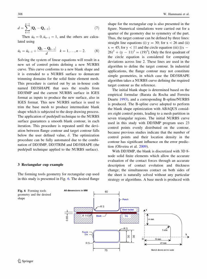
The forming tools geometry for rectangular cup used

in this study is presented in Fig. 6. The desired flange

shape for the rectangular cup is also presented in the

figure. Numerical simulations were carried out for a

quarter of the geometry due to symmetry of the part.

Thus, the target contour can be defined by three lines:

straight line equations (i) y = 30; for x \ 26 and (ii)

x = 45; for y \ 11 and the circle equation (iii) [(x -

26)2 ? (y - 11)2 = (19)2]. Only the first quadrant of

the circle equation is considered for computing

deviations across line 2. These lines are used in the

algorithm to define the target contour. In industrial

applications, the flange contour may not constitute

simple geometries, in which case the DD3SHAPE

algorithm takes a NURBS curve defining the required

target contour as the reference.

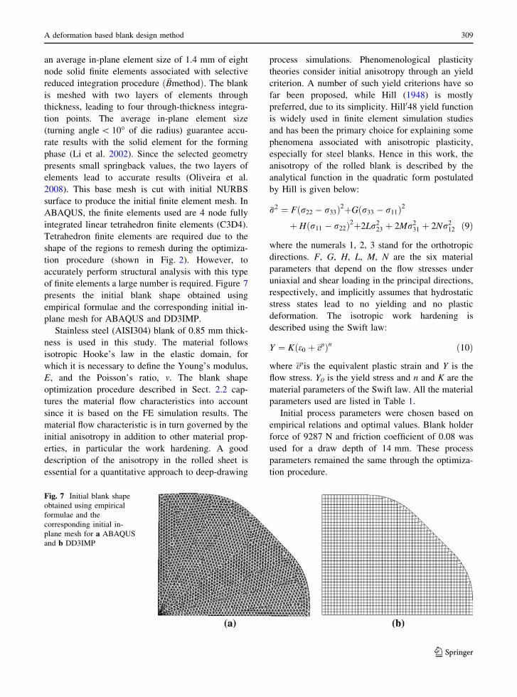
The initial blank shape is determined based on the

empirical formulae (Barata da Rocha and Ferreira

Duarte 1993), and a corresponding B-spline/NURBS

is produced. The B-spline curve adopted to perform

the blank shape optimization with ABAQUS consid-

ers eight control points, leading to a mesh partition in

seven triangular regions. The initial NURBS curve

used in this study with DD3IMP program uses 23

control points evenly distributed on the contour,

because previous studies indicate that the number of

control points and their location density in the

contour has significant influence on the error predic-

tion (Oliveira et al. 2009).

With DD3IMP, the blank is discretized with 3D 8-

node solid finite elements which allow the accurate

evaluation of the contact forces through an accurate

description of contact evolution and thickness

change; the simultaneous contact on both sides of

the sheet is naturally solved without any particular

strategy or algorithms. A base mesh is produced with

Fig. 6 Forming tools

geometry and the desired

shape

308 W. Hammami et al.

123

an average in-plane element size of 1.4 mm of eight

node solid finite elements associated with selective

reduced integration procedure ð �BmethodÞ. The blank

is meshed with two layers of elements through

thickness, leading to four through-thickness integra-

tion points. The average in-plane element size

(turning angle \ 10� of die radius) guarantee accu-

rate results with the solid element for the forming

phase (Li et al. 2002). Since the selected geometry

presents small springback values, the two layers of

elements lead to accurate results (Oliveira et al.

2008). This base mesh is cut with initial NURBS

surface to produce the initial finite element mesh. In

ABAQUS, the finite elements used are 4 node fully

integrated linear tetrahedron finite elements (C3D4).

Tetrahedron finite elements are required due to the

shape of the regions to remesh during the optimiza-

tion procedure (shown in Fig. 2). However, to

accurately perform structural analysis with this type

of finite elements a large number is required. Figure 7

presents the initial blank shape obtained using

empirical formulae and the corresponding initial in-

plane mesh for ABAQUS and DD3IMP.

Stainless steel (AISI304) blank of 0.85 mm thick-

ness is used in this study. The material follows

isotropic Hooke’s law in the elastic domain, for

which it is necessary to define the Young’s modulus,

E, and the Poisson’s ratio, m. The blank shape

optimization procedure described in Sect. 2.2 cap-

tures the material flow characteristics into account

since it is based on the FE simulation results. The

material flow characteristic is in turn governed by the

initial anisotropy in addition to other material prop-

erties, in particular the work hardening. A good

description of the anisotropy in the rolled sheet is

essential for a quantitative approach to deep-drawing

process simulations. Phenomenological plasticity

theories consider initial anisotropy through an yield

criterion. A number of such yield criterions have so

far been proposed, while Hill (1948) is mostly

preferred, due to its simplicity. Hill048 yield function

is widely used in finite element simulation studies

and has been the primary choice for explaining some

phenomena associated with anisotropic plasticity,

especially for steel blanks. Hence in this work, the

anisotropy of the rolled blank is described by the

analytical function in the quadratic form postulated

by Hill is given below:

�r2 ¼ F r22 � r33ð Þ2þG r33 � r11ð Þ2

þ H r11 � r22ð Þ2þ2Lr223 þ 2Mr2

31 þ 2Nr212 ð9Þ

where the numerals 1, 2, 3 stand for the orthotropic

directions. F, G, H, L, M, N are the six material

parameters that depend on the flow stresses under

uniaxial and shear loading in the principal directions,

respectively, and implicitly assumes that hydrostatic

stress states lead to no yielding and no plastic

deformation. The isotropic work hardening is

described using the Swift law:

Y ¼ K e0 þ �epð Þn ð10Þ

where �epis the equivalent plastic strain and Y is the

flow stress. Y0 is the yield stress and n and K are the

material parameters of the Swift law. All the material

parameters used are listed in Table 1.

Initial process parameters were chosen based on

empirical relations and optimal values. Blank holder

force of 9287 N and friction coefficient of 0.08 was

used for a draw depth of 14 mm. These process

parameters remained the same through the optimiza-

tion procedure.

Fig. 7 Initial blank shape

obtained using empirical

formulae and the

corresponding initial in-

plane mesh for a ABAQUS

and b DD3IMP

A deformation based blank design method 309

123

4 Discussion on results

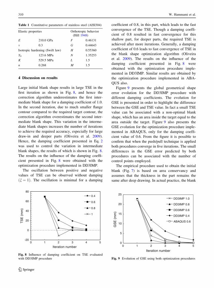
Large initial blank shape results in large TSE in the

first iteration as shown in Fig. 8, and hence the

correction algorithm underestimates the first inter-

mediate blank shape for a damping coefficient of 1.0.

In the second iteration, due to much smaller flange

contour compared to the required target contour, the

correction algorithm overestimates the second inter-

mediate blank shape. This variation in the interme-

diate blank shapes increases the number of iterations

to achieve the required accuracy, especially for large

draw-in and deeper parts (Oliveira et al. 2009).

Hence, the damping coefficient presented in Eq. 2

was used to control the variation in intermediate

blank shapes, the results of which is shown in Fig. 8.

The results on the influence of the damping coeffi-

cient presented in Fig. 8 were obtained with the

optimization procedure implemented in DD3IMP.

The oscillation between positive and negative

values of TSE can be observed without damping

n ¼ 1ð Þ. The oscillation is minimal for a damping

coefficient of 0.8, in this part, which leads to the fast

convergence of the TSE. Though a damping coeffi-

cient of 0.8 resulted in fast convergence for this

shallow part, for deeper parts, the required TSE is

achieved after more iterations. Generally, a damping

coefficient of 0.6 leads to fast convergence of TSE in

the blank shape optimization algorithm (Oliveira

et al. 2009). The results on the influence of the

damping coefficient presented in Fig. 8 were

obtained with the optimization procedure imple-

mented in DD3IMP. Similar results are obtained by

the optimization procedure implemented in ABA-

QUS also.

Figure 9 presents the global geometrical shape

error evolution for the DD3IMP procedure with

different damping coefficients. The evolution for

GSE is presented in order to highlight the difference

between the GSE and TSE value. In fact a small TSE

value can be associated with a non-optimal blank

shape, which has an area inside the target equal to the

area outside the target. Figure 9 also presents the

GSE evolution for the optimization procedure imple-

mented in ABAQUS, only for the damping coeffi-

cient value of 0.6. From the figure it is possible to

confirm that when the push/pull technique is applied

both procedures converge in five iterations. The small

differences in the GSE error predicted by both

procedures can be associated with the number of

control points employed.

The empirical procedure used to obtain the initial

blank (Fig. 7) is based on area conservancy and

assumes that the thickness in the part remains the

same after deep drawing. In actual practice, the blank

Table 1 Constitutive parameters of stainless steel (AISI304)

Elastic properties Orthotropic behavior

(Hill 1948)

E 210.0 GPa F 0.46131

m 0.3 G 0.44643

Isotropic hardening (Swift law) H 0.55360

Y0 123.6 MPa N 1.35253

K 529.5 MPa L 1.5

n 0.268 M 1.5

-20

0

20

40

60

80

0 1 2 3 4 5

Iteration number

TS

E (

mm

)

0.4

0.6

0.8

1

Fig. 8 Influence of damping coefficient on TSE evaluated

with DD3IMP procedure

0

5

10

15

20

25

0 1 2 3 4 5

Iteration number

GS

E (

mm

)

DD3IMP 1.0

DD3IMP 0.8

DD3IMP 0.6

DD3IMP 0.4

ABAQUS 0.6

Fig. 9 Evolution of GSE using both optimization procedures

310 W. Hammami et al.

123

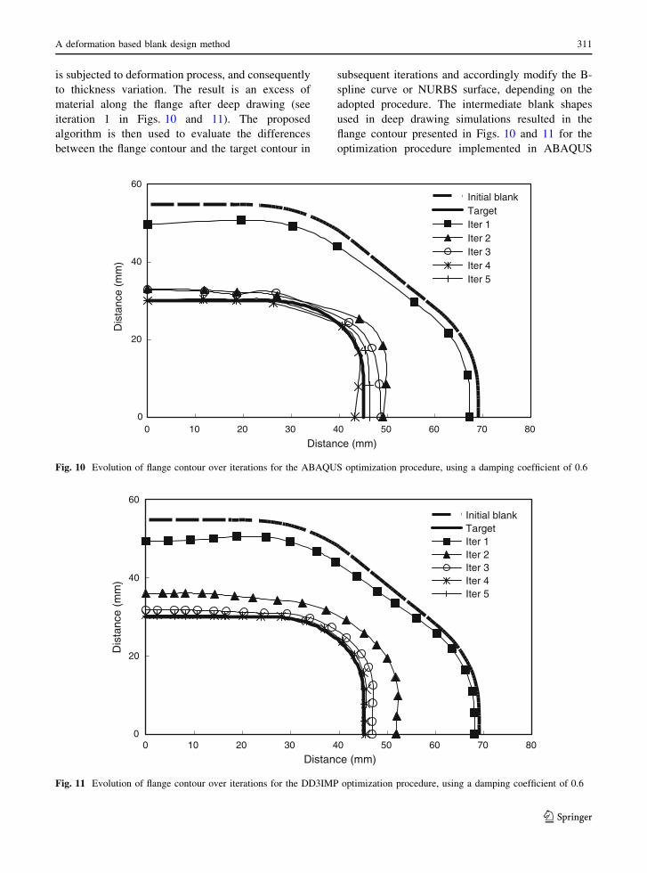
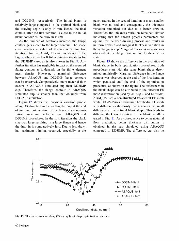
is subjected to deformation process, and consequently

to thickness variation. The result is an excess of

material along the flange after deep drawing (see

iteration 1 in Figs. 10 and 11). The proposed

algorithm is then used to evaluate the differences

between the flange contour and the target contour in

subsequent iterations and accordingly modify the B-

spline curve or NURBS surface, depending on the

adopted procedure. The intermediate blank shapes

used in deep drawing simulations resulted in the

flange contour presented in Figs. 10 and 11 for the

optimization procedure implemented in ABAQUS

0

20

40

60

0 10 20 30 40 50 60 70 80

Distance (mm)

Dis

tanc

e (m

m)

Initial blankTargetIter 1Iter 2Iter 3Iter 4Iter 5

Fig. 10 Evolution of flange contour over iterations for the ABAQUS optimization procedure, using a damping coefficient of 0.6

0

20

40

60

0 10 20 30 40 50 60 70 80

Distance (mm)

Dis

tanc

e (m

m)

Initial blankTargetIter 1Iter 2Iter 3Iter 4Iter 5

Fig. 11 Evolution of flange contour over iterations for the DD3IMP optimization procedure, using a damping coefficient of 0.6

A deformation based blank design method 311

123

and DD3IMP, respectively. The initial blank is

relatively large compared to the optimal blank and

the drawing depth is only 14 mm. Hence, the final

contour after the first iteration is close to the initial

blank contour as the draw-in is small.

As the number of iterations increase, the flange

contour gets closer to the target contour. The shape

error reaches a value of 0.204 mm within five

iterations for the ABAQUS case, as shown in the

Fig. 9, while it reaches 0.164 within five iterations for

the DD3IMP case, as is also shown in Fig. 9. Any

further iteration has negligible impact on the required

flange contour as it depends on the finite element

mesh density. However, a marginal difference

between ABAQUS and DD3IMP flange contours

can be observed. Comparatively, more material flow

occurs in ABAQUS simulated cup than DD3IMP

cup. Therefore, the flange contour in ABAQUS

simulated cup is smaller than that obtained from

DD3IMP simulation.

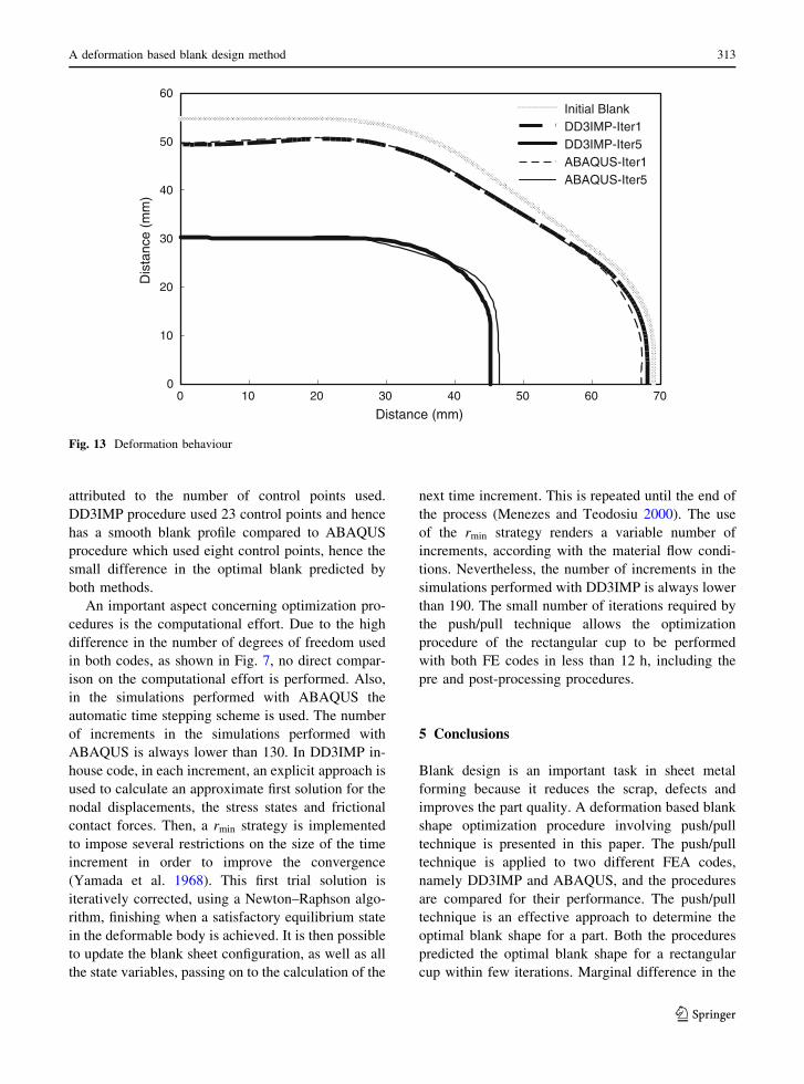
Figure 12 shows the thickness variation profile

along OX direction in the rectangular cup at the end

of first and last iteration of the blank shape optimi-

zation procedure, performed with ABAQUS and

DD3IMP procedures. In the first iteration the blank

size was large resulting in a large flange and hence

the draw-in is comparatively less. Due to less draw-

in, maximum thinning occurred, especially at the

punch radius. In the second iteration, a much smaller

blank was utilised and consequently the thickness

variation smoothed out due to a better draw-in.

Thereafter, the thickness variation remained similar

indicating that the chosen process parameters are

optimal for the deep drawing process and results in

uniform draw-in and marginal thickness variation in

the rectangular cup. Marginal thickness increase was

observed at the flange contour due to shear stress

state.

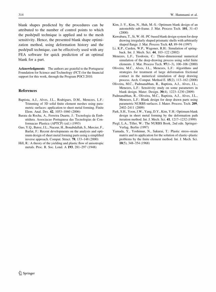
Figure 13 shows the difference in the evolution of

blank shape in both optimization procedures. Both

procedures start with the same blank shape deter-

mined empirically. Marginal difference in the flange

contour was observed at the end of the first iteration

which persisted until the end of the optimization

procedure, as shown in the figure. The differences in

the blank shape can be attributed to the different FE

mesh discretization used by ABAQUS and DD3IMP.

ABAQUS uses a non-structured tetrahedral FE mesh

while DD3IMP uses a structured hexahedral FE mesh

with different mesh density that generates the small

difference in the optimal blank shape. This leads to

different thickness evolution in the blank, as illus-

trated in Fig. 11. As a consequence to better material

flow prediction, better thickness distribution is

obtained in the cup simulated using ABAQUS

compared to DD3IMP. The difference can also be

0.8

0.9

1

1.1

0 20 40 60 80

Curvilinear distance (mm)

Thi

ckne

ss (

mm

)

DD3IMP-Iter1

DD3IMP-Iter5

ABAQUS-Iter1

ABAQUS-Iter5

Fig. 12 Thickness evolution along OX during blank shape optimization procedure

312 W. Hammami et al.

123

attributed to the number of control points used.

DD3IMP procedure used 23 control points and hence

has a smooth blank profile compared to ABAQUS

procedure which used eight control points, hence the

small difference in the optimal blank predicted by

both methods.

An important aspect concerning optimization pro-

cedures is the computational effort. Due to the high

difference in the number of degrees of freedom used

in both codes, as shown in Fig. 7, no direct compar-

ison on the computational effort is performed. Also,

in the simulations performed with ABAQUS the

automatic time stepping scheme is used. The number

of increments in the simulations performed with

ABAQUS is always lower than 130. In DD3IMP in-

house code, in each increment, an explicit approach is

used to calculate an approximate first solution for the

nodal displacements, the stress states and frictional

contact forces. Then, a rmin strategy is implemented

to impose several restrictions on the size of the time

increment in order to improve the convergence

(Yamada et al. 1968). This first trial solution is

iteratively corrected, using a Newton–Raphson algo-

rithm, finishing when a satisfactory equilibrium state

in the deformable body is achieved. It is then possible

to update the blank sheet configuration, as well as all

the state variables, passing on to the calculation of the

next time increment. This is repeated until the end of

the process (Menezes and Teodosiu 2000). The use

of the rmin strategy renders a variable number of

increments, according with the material flow condi-

tions. Nevertheless, the number of increments in the

simulations performed with DD3IMP is always lower

than 190. The small number of iterations required by

the push/pull technique allows the optimization

procedure of the rectangular cup to be performed

with both FE codes in less than 12 h, including the

pre and post-processing procedures.

5 Conclusions

Blank design is an important task in sheet metal

forming because it reduces the scrap, defects and

improves the part quality. A deformation based blank

shape optimization procedure involving push/pull

technique is presented in this paper. The push/pull

technique is applied to two different FEA codes,

namely DD3IMP and ABAQUS, and the procedures

are compared for their performance. The push/pull

technique is an effective approach to determine the

optimal blank shape for a part. Both the procedures

predicted the optimal blank shape for a rectangular

cup within few iterations. Marginal difference in the

0

10

20

30

40

50

60

0 10 20 30 40 50 60 70

Distance (mm)

Dis

tanc

e (m

m)

Initial BlankDD3IMP-Iter1DD3IMP-Iter5ABAQUS-Iter1ABAQUS-Iter5

Fig. 13 Deformation behaviour

A deformation based blank design method 313

123

blank shapes predicted by the procedures can be

attributed to the number of control points to which

the push/pull technique is applied and to the mesh

sensitivity. Hence, the presented blank shape optimi-

zation method, using deformation history and the

push/pull technique, can be effectively used with any

FEA software for quick prediction of an optimal

blank for a part.

Acknowledgments The authors are grateful to the Portuguese

Foundation for Science and Technology (FCT) for the financial

support for this work, through the Program POCI 2010.

References

Baptista, A.J., Alves, J.L., Rodrigues, D.M., Menezes, L.F.:

Trimming of 3D solid finite element meshes using para-

metric surfaces: application to sheet metal forming. Finite

Elem. Anal. Des. 42, 1053–1060 (2006)

Barata da Rocha, A., Ferreira Duarte, J.: Tecnologia da Emb-

utidura. Associacao Portuguesa das Tecnologias de Con-

formacao Plastica (APTCP) (ed.) (1993)

Guo, Y.Q., Batoz, J.L., Naceur, H., Bouabdallah, S., Mercier, F.,

Barlat, F.: Recent developments on the analysis and opti-

mum design of sheet metal forming parts using a simplified

inverse approach. Comput. Struct. 78, 133–148 (2000)

Hill, R.: A theory of the yielding and plastic flow of anisotropic

metals. Proc. R. Soc. Lond. A 193, 281–297 (1948)

Kim, J.-Y., Kim, N., Huh, M.-S.: Optimum blank design of an

automobile sub-frame. J. Mat. Process Tech. 101, 31–43

(2000)

Kuwabara, T., Si, W.-H.: PC-based blank design system for deep

drawing irregularly shaped prismatic shells with arbitrarily

shaped flange. J. Mat. Process Tech. 63, 89–94 (1997)

Li, K.P., Carden, W.P., Wagoner, R.H.: Simulation of spring-

back. Int. J. Mech. Sci. 44, 103–122 (2002)

Menezes, L.F., Teodosiu, C.: Three-dimensional numerical

simulation of the deep-drawing process using solid finite

elements. J. Mat. Process Tech. 97(1–3), 100–106 (2000)

Oliveira, M.C., Alves, J.L., Menezes, L.F.: Algorithms and

strategies for treatment of large deformation frictional

contact in the numerical simulation of deep drawing

process. Arch. Comput. Method E. 15(2), 113–162 (2008)

Oliveira, M.C., Padmanabhan, R., Baptista, A.J., Alves, J.L.,

Menezes, L.F.: Sensitivity study on some parameters in

blank design. Mater. Design. 30(4), 1223–1230 (2009)

Padmanabhan, R., Oliveira, M.C., Baptista, A.J., Alves, J.L.,

Menezes, L.F.: Blank design for deep drawn parts using

parametric NURBS surfaces. J. Mater. Process. Tech. 209,

2402–2411 (2009)

Park, S.H., Yoon, J.W., Yang, D.Y., Kim, Y.H.: Optimum blank

design in sheet metal forming by the deformation path

iteration method. Int. J. Mech. Sci. 41, 1217–1232 (1999)

Piegl, L.A., Tiller, W.: The NURBS Book, 2nd edn. Springer-

Verlag, Berlin (1997)

Yamada, Y., Yoshimur, N., Sakurai, T.: Plastic stress–strain

matrix and its application for the solution of elastic–plastic

problems by the finite element method. Int. J. Mech. Sci.

10(5), 348–354 (1968)

314 W. Hammami et al.

123