A DELAY REACTION-DIFFUSION MODEL OF THESPREAD OF BACTERIOPHAGE INFECTION∗

STEPHEN A. GOURLEY† AND YANG KUANG‡

SIAM J. APPL. MATH. c© 2005 Society for Industrial and Applied MathematicsVol. 65, No. 2, pp. 550–566

Abstract. This paper is a continuation of recent attempts to understand, via mathematicalmodeling, the dynamics of marine bacteriophage infections. Previous authors have proposed systemsof ordinary differential delay equations with delay dependent coefficients. In this paper we continuethese studies in two respects. First, we show that the dynamics is sensitive to the phage mortalityfunction, and in particular to the parameter we use to measure the density dependent phage mortalityrate. Second, we incorporate spatial effects by deriving, in one spatial dimension, a delay reaction-diffusion model in which the delay term is rigorously derived by solving a von Foerster equation.Using this model, we formally compute the speed at which the viral infection spreads through thedomain and investigate how this speed depends on the system parameters. Numerical simulationssuggest that the minimum speed according to linear theory is the asymptotic speed of propagation.

Key words. reaction-diffusion, delay, stage structure, through-stage death rate, traveling wave

AMS subject classifications. 92D25, 35K57, 35R10

DOI. 10.1137/S0036139903436613

1. Introduction. It is known that bacteriophage infection can be a signifi-cant mechanism of mortality in marine prokaryotes (Bergh et al. [6], Proctor andFuhrman [16]). These mortality mechanisms are critical in understanding the marineproduction processes. The constituents released by cell lysis can be an importantpathway of nutrient recycling. This has direct bearing on issues such as global warm-ing and topics of geochemical cycles. Viral infection also has direct implications forgenetic exchange in the sea (Lenski and Levin [14], Bohannan and Lenski [7]).

Although we do not yet have a good understanding of the temporal or spatialscales at which host-virus encounters occur, it is clear that viral mortality must beexplicitly considered in most models of the marine system. A case in point, recentexperimental work suggests that the contamination of algal cells by viruses can serveas a regulatory mechanism in its bloom dynamics. Beltrami and Carroll [1] formulateda simple trophic model including virus-induced mortality. Their model succeeded inmimicking the actual algal bloom patterns of several species.

Our main interest in this paper is to explore how viral mortality affects boththe temporal and spatial dynamics of marine bacteria and cyanobacteria. Recently,Beretta and Kuang [4] formulated and carried out a detailed study of the temporalviral-bacteria model

dSdt

= αS(t)

(1 − S(t) + I(t)

C

)−KS(t)P (t),

dIdt

= −µiI(t) + KS(t)P (t) − e−µiTKS(t− T )P (t− T ),

dPdt

= β − µpP (t) −KS(t)P (t) + be−µiTKS(t− T )P (t− T ).

(1.1)

∗Received by the editors October 24, 2003; accepted for publication (in revised form) May 17,2004; published electronically January 5, 2005.

http://www.siam.org/journals/siap/65-2/43661.html†Corresponding author. Department of Mathematics and Statistics, University of Surrey, Guild-

ford, Surrey GU2 7XH, UK (s.gourley@surrey.ac.uk). Correspondence should be directed to thisauthor.

‡Department of Mathematics and Statistics, Arizona State University, Tempe, AZ 85287 (kuang@asu.edu). The research of this author was partially supported by NSF grant DMS-0077790.

550

SPATIAL SPREAD OF BACTERIOPHAGE INFECTION 551

This system of delay differential equations models a population of marine bacteria inwhich the individuals are subject to infection by viruses, also known as bacteriophages.Prior to that, these authors (Beretta and Kuang [2]) modeled and studied the sameprocess by a set of nonlinear ordinary differential equations, and Carletti [10] hasstudied the stochastic extension of that model. In system (1.1), S is the density(i.e., number of bacteria per liter) of susceptible bacteria, I is the density of infectedbacteria, and P is the density (number of viruses per liter) of viruses (phages). VirusesP attack the susceptible bacteria S, and a bacterium becomes infected I when a virussuccessfully injects itself through the bacterial membrane. The virus then startsreplicating inside the bacterium, and then all the bacterium’s resources are directedto replication of the virus. The infected bacterium does not replicate itself by division;only susceptible bacteria are capable of doing so. After a latency time T , an infectedbacterium will die by lysis; i.e., the bacterium explodes releasing b copies (b > 1) ofthe virus into the solution, which are then free to attack other susceptible bacteria.An infected bacterium may die other than by viral lysis; we allow for this by the term−µiI(t). The differential equation for I(t) is derived from the fact that I(t) is givenby

I(t) =

∫ T

0

e−µiτKS(t− τ)P (t− τ) dτ,(1.2)

which expresses the fact that the number of recruits into the infected class betweentimes t − (τ + dτ) and t − τ is KS(t − τ)P (t − τ) dτ , the number of these still aliveat time t is obtained by multiplying by e−µiτ , and then the integral totals up thecontributions from all relevant previous times, i.e., up to T time units ago.

In the virus equation, the third equation of (1.1), all mortalities of viruses areaccounted for by the term −µpP (t). The β term, where β > 0, models a constantinflow of phages from outside the system. In the absence of viruses the bacteria growlogistically. The rate of infection is given by the law of mass action to be KS(t)P (t).

Beretta and Kuang [4] assumed that infected bacteria still compete with suscep-tible bacteria for common resources. This is represented by the −(S + I)/C term inthe first equation of (1.1). This is clearly a disputed subject. For example, a modelby Campbell [8] consists of the following equations:

dS(t)

dt= αS(t)

(1 − S(t)

C

)−KS(t)P (t),(1.3)

dP (t)

dt= bKS(t− T )P (t− T ) − µpP (t) −KS(t)P (t),

where

I(t) =

∫ t

t−T

KS(θ)P (θ)dθ.(1.4)

Clearly, in (1.3) the competition for common resources and additional mortality rateendured by infected bacteria is neglected. The equations (1.3), (1.4) can be obtainedfrom (1.1) by setting β = 0, µi = 0. Extensions of the above Campbell model canbe found in Beretta, Carletti, and Solimano [3] (taking into account environmentalfluctuations) and Carletti [9] (replacing b by be−µiT ).

In the present paper, like the model of Campbell [8], we assume that once abacterium becomes infected by a virus, it no longer competes with susceptibles for

552 STEPHEN A. GOURLEY AND YANG KUANG

resources. We will allow the possibility of a density dependent mortality term in thephage equation. In Beretta and Kuang [4], and also in the present paper, it is assumedthat T and b are constant and the same for the whole population. Modifications ofthis assumption (e.g., replacing the constant incubation time T by a distribution ofincubation times modeled using a probability density function) are the subject offurther work presently in progress.

In the next section, we will present our delay model of bacteriophage infectionand a simple preliminary result on the positivity of its solutions. This is followed bya short section on the global stability of the disease-free equilibrium. The analysisof endemic equilibrium is highly nontrivial and we provide only generic conditionsfor its stability switch. To complement this analytic work, we present some carefullydesigned and data-based simulation results. We then proceed to formulate and studya delay reaction-diffusion model of the spread of bacteriophage infection. The paperends with a discussion.

2. Preliminaries. Most of our effort will be devoted to understanding the sys-tem

S′(t) = αS(t)(1 − S(t)

γ

)−KS(t)P (t),

P ′(t) = −µpP (t) −mP 2(t) −KS(t)P (t) + bKe−µiTS(t− T )P (t− T ),(2.1)

and with a reaction-diffusion version of (2.1). The initial conditions for (2.1) are

S(s) = S0(s) ≥ 0, s ∈ [−T, 0], with S0(0) > 0,P (s) = P 0(s) ≥ 0, s ∈ [−T, 0], with P 0(0) > 0,

(2.2)

where S0 and P 0 are prescribed continuous functions. Our system (2.1) differs fromthat studied in [4] in three respects: (i) we do not have an inflow of phages fromoutside the system, (ii) we allow the possibility of a density dependent mortality term(the term −mP 2 in (2.1)), and (iii) we assume that an infected bacterium no longercompetes with the susceptibles for resources. The latter assumption means that wedo not need the differential equation for I(t) for the analysis (though I(t) is still givenby (1.2)). An additional difference is that in the present paper we shall consider theeffects of including diffusion to model the motion of the phages and bacteria.

If we had P 0(s) ≡ 0 on [−T, 0], the method of steps would immediately yieldP (t) = 0 for all t > 0. The dynamics of S(t) would then be governed by the logisticequation. Similarly, if S0(s) ≡ 0, then clearly S(t) remains zero for all t > 0 andthus P (t)→0 as t→∞. These trivial cases are removed from consideration by theassumptions in (2.2).

Proposition 1. Solutions of (2.1), (2.2) satisfy S(t) > 0, P (t) > 0 for all t > 0.Proof. The equation for S(t) in (2.1) contains a factor of S(t) and therefore

positivity for S(t) follows by the standard argument. For P (t), note that on t ∈ [0, T ]we have P ′(t) ≥ −µpP (t) − mP 2(t) − KS(t)P (t) so that P (t) ≥ P (t), where P is

the solution of P ′(t) = −µpP (t) −mP 2(t) −KS(t)P (t) satisfying P (0) = P (0) > 0.

Clearly P (t) > 0 for all t > 0, and so we conclude that P (t) > 0 for all t > 0. Theproof is complete.

3. Equilibria and their stability. The equilibria of (2.1) are (S, P ) = (0, 0),the disease-free equilibrium (γ, 0), and possibly an endemic equilibrium

(S∗, P ∗) :=

(mγα + Kγµp

mα + K2γ(be−µiT − 1),αγK(be−µiT − 1) − αµp

mα + K2γ(be−µiT − 1)

).(3.1)

SPATIAL SPREAD OF BACTERIOPHAGE INFECTION 553

The latter is ecologically relevant if and only if

be−µiT > 1 +µp

γK,(3.2)

which, of course, can only possibly hold for T up to a finite value. As long as (3.2)holds, there is an endemic equilibrium. Note that as m→∞ the endemic equilibriumapproaches the disease-free equilibrium (γ, 0).

We shall first prove that, if condition (3.2) does not hold, then any positivesolution approaches the disease-free equilibrium (γ, 0).

Theorem 1. Assume that

be−µiT ≤ 1 +µp

γK.

Then any solution of (2.1), (2.2) satisfies

limt→∞

(S(t), P (t)) = (γ, 0).

Proof. Consider the positive definite functional

V = S − γ − γ lnS

γ+

γK

µpP +

bγK2

µpe−µiT

∫ t

t−T

S(s)P (s) ds.

Differentiating along solutions of (2.1) yields

V ′ = −α

γ(S − γ)2 − γmK

µpP 2 + K

(bγK

µpe−µiT − γK

µp− 1

)SP

≤ −α

γ(S − γ)2.

Thus

V (t) +α

γ

∫ t

0

(S(s) − γ)2 ds ≤ V (0),

and, letting t→∞, we conclude that |S(t) − γ| ∈ L2(0,∞) so that S(t)→γ as t→∞.The differential equations (2.1) then yield P (t)→0. The proof is complete.

3.1. The endemic equilibrium: Linearized analysis. Let us investigate theendemic equilibrium (S∗, P ∗) given by (3.1). In this subsection we shall assume, ofcourse, that (3.2) holds, so that the equilibrium is feasible. The linearized analysisabout the endemic equilibrium is algebraically quite complicated. The main reasonfor this is that the delay T appears not only in the S(t − T )P (t − T ) term in thesecond equation of (2.1), but also in the factor e−µiT in front of that term. Thepaper by Wolkowicz, Xia, and Wu [20] shows how such additional factors involvingtime delay can appear in distributed delay equations. Surprisingly, this representsa significant complication and prevents us from analytically computing the preciseparameter regimes in which the endemic equilibrium can change stability as the delayT is increased, or the actual values of T when stability switches occur. Note furtherthat the equilibrium itself depends on T and exists only for T up to a finite value.This renders many of the existing stability switch methods (see Kuang [12]) powerless.However, a method has recently been developed by Beretta and Kuang [5] to addressthe problem of computing stability switches for delay equations which do not lend

554 STEPHEN A. GOURLEY AND YANG KUANG

themselves to classical methods because of these complications. We shall use thismethod in this section.

To linearize about (S∗, P ∗) we set S = S∗ + S and P = P ∗ + P . Ignoring higherorder terms in S, P gives us the linearized system

S′(t) = −αγ S

∗S(t) −KS∗P (t),

P ′(t) = −KP ∗S(t) − (µp + 2mP ∗ + KS∗)P (t)

+ bKe−µiT (P ∗S(t− T ) + S∗P (t− T )).

(3.3)

We shall find it convenient to introduce the parameter

ρT =γK

µp(be−µiT − 1).(3.4)

Then the endemic equilibrium (S∗, P ∗) exists if and only if

ρT > 1.

In terms of ρT ,

(S∗, P ∗) =

(γ(mα + Kµp)

mα + KµpρT,

αµp(ρT − 1)

mα + KµpρT

).

Nontrivial solutions of the linearized system of the form (S(t), P (t)) = eλt(c1, c2) existif and only if

D(λ;T ) = 0,

where

D(λ;T ) = λ2 + a(T )λ + b(T )λe−λT + c(T ) + d(T )e−λT(3.5)

and

a(T ) =α(mα + Kµp) + mα(Kγ + 2µpρT − µp) + Kµp(Kγ + µpρT )

mα + KµpρT,(3.6)

b(T ) = −bγKe−µiT (mα + Kµp)

mα + KµpρT,(3.7)

c(T ) =α(mα + Kµp) {mα(Kγ + (2ρT − 1)µp) + Kµp(µpρT + (2 − ρT )Kγ)}

(mα + KµpρT )2,(3.8)

d(T ) =bKγαe−µiT (mα + Kµp) {Kµp(ρT − 2) −mα}

(mα + KµpρT )2.(3.9)

Keeping in mind that b > 1, it is straightforward to see that when T = 0 the equilib-rium (S∗, P ∗), if feasible, is linearly stable. This is because when T = 0, (3.5) becomesa quadratic in λ, and it is easy to see that a(0) + b(0) > 0 and c(0) + d(0) > 0. Thequestion is whether the equilibrium can undergo any stability switch as T is increased,remembering that the equilibrium is only feasible up to a finite value of T . To identifya stability switch we seek solutions of the characteristic equation D(λ;T ) = 0 of the

SPATIAL SPREAD OF BACTERIOPHAGE INFECTION 555

form λ = ±iω, with ω a real positive number. We find that it is necessary for ω tosatisfy

ω4 + (a2(T ) − 2c(T ) − b2(T ))ω2 + c2(T ) − d2(T ) = 0.(3.10)

However, the existence for a particular T of a real root ω(T ) of (3.10) does not initself imply that a stability switch occurs at that value of T , since T also has tosatisfy (3.11) and (3.12) below. Nonetheless, certain general analytical conclusionscan be drawn in spite of the algebra. Straightforward but tedious computations showthat, for any parameter values consistent with ρT > 1 (i.e., with existence of theendemic equilibrium (S∗, P ∗)), we have

a2(T ) − 2c(T ) − b2(T ) > 0.

In light of this fact, and assuming that (S∗, P ∗) is feasible when T = 0, certainconclusions follow.

(i) A stability switch cannot occur in an interval of T throughout which c2(T ) >d2(T ).

(ii) If there are values of T with c2(T ) < d2(T ), then a stability switch may occuras T is varied. Pairs of eigenvalues cross the imaginary axis as T passes throughcertain critical values. The critical values of T and the corresponding purely imaginaryeigenvalues ±iω(T ), ω(T ) > 0, are given implicitly by

sin(ω(T )T ) =b(T )ω(T )(ω2(T ) − c(T )) + ω(T )a(T )d(T )

ω2(T )b2(T ) + d2(T ),(3.11)

cos(ω(T )T ) =d(T )(ω2(T ) − c(T )) − ω2(T )a(T )b(T )

ω2(T )b2(T ) + d2(T ),(3.12)

ω2(T ) =1

2

(− a2(T ) + 2c(T ) + b2(T )(3.13)

+√a4(T ) − 4a2(T )c(T ) − 2a2(T )b2(T ) + 4c(T )b2(T ) + b4(T ) + 4d2(T )

),

where a(T ), b(T ), c(T ), and d(T ) are given by (3.6), (3.7), (3.8), and (3.9) above. Itis impossible to solve these equations for T explicitly, so we shall use the proceduredescribed in Beretta and Kuang [5]. According to this procedure, we define θ(T ) ∈[0, 2π) such that sin θ(T ) and cos θ(T ) are given by the right-hand sides of (3.11)and (3.12), respectively, with ω(T ) given by (3.13). This defines θ(T ) in a formsuitable for numerical evaluation using standard software. Then T is given (stillimplicitly) by

T =θ(T ) + 2nπ

ω(T ), n = 0, 1, 2, . . . ,

and the idea is to identify the roots of this equation for various n, i.e., to solvenumerically the equation Sn(T ) = 0 for n = 0, 1, 2, where

Sn(T ) = T −(θ(T ) + 2nπ

ω(T )

), n = 0, 1, 2, . . . .(3.14)

556 STEPHEN A. GOURLEY AND YANG KUANG

Accurate plots of these functions Sn(T ) quickly reveal whether stability switches canoccur or not, but one must remember to keep track of the feasibility of the equilibrium(S∗, P ∗) since it disappears completely (by coalescing with the disease-free equilibrium(γ, 0)) at a finite value of the delay T .

By reference to (i) above, it is possible to obtain sufficient and easily verifiableconditions for the equilibrium (S∗, P ∗) to remain locally stable. Indeed, the conditionc2(T ) > d2(T ) amounts to

(3.15)

m2{α2(Kγ + (2ρT − 1)µp)

2 − α2b2K2γ2e−2µiT}

+ 2αKµpm{(Kγ + (2ρT − 1)µp)(µpρT + (2 − ρT )Kγ) + (ρT − 2)b2K2γ2e−2µiT

}+ K2µ2

p(µpρT + (2 − ρT )Kγ)2 −K2µ2p(ρT − 2)2b2K2γ2e−2µiT > 0.

Thus, if (3.15) holds, then (S∗, P ∗), if feasible, is locally stable. The coefficient of m2

in (3.15) is automatically positive if ρT > 1 (the condition for feasibility of (S∗, P ∗)),and therefore one parameter regime in which (3.15) is satisfied is that the parameterm be large.

For the convenience of comparison and computation, we perform the same di-mensionless analysis as was carried out in Beretta and Kuang [4]. We choose thedimensionless time as τ = Kγt. Note that one unit of the dimensionless time scale,i.e., τ = 1, corresponds to tτ = (1/Kγ) in the original time unit. We also need thedimensionless variables

s =S

γ, p =

P

γ.

Below are the dimensionless parameters:

a =α

Kγ, mp =

µp

Kγ, mi =

µi

Kγ, mq =

m

K.

Equations (2.1) have the dimensionless form⎧⎪⎪⎨⎪⎪⎩ds(τ)

dτ= as(τ) − as2(τ) − s(τ)p(τ),

dp(τ)

dτ= −mpp(τ) −mqp

2(τ) − s(τ)p(τ) + be−miTτ s(τ − Tτ )p(τ − Tτ ).(3.16)

The values for the dimensionless parameters and the dimensionless time scale aretaken from the model of Beretta and Kuang [4] (the original parameter estimates aredue to Okubo). They are

a = 10, mp = 14.925,(3.17)

with tτ = (1/Kγ) = 7.4627 days and an average latency time T � 0.303 days. Wehave no estimates for mi = (µi/Kγ), but it seems reasonable to assume it is smallerthan m (since the main cause of mortality is the lysis of infected cells). We assumemi � 0.1mp. In addition, we do not have an estimate on mq. In the followingcomputational work, we assume that mq � 0.1, a value close to zero. Figure 1 is theresult of an application of the stability switch theory of Beretta and Kuang [5] forthis set of parameters (except that we vary the latency period).

Figure 2 provides simulation results for the above set of parameters with four rep-resentative values of latency periods. Clearly Figure 2 confirms the findings embodiedin Figure 1.

SPATIAL SPREAD OF BACTERIOPHAGE INFECTION 557

Graph of stability switch for S_0(T) and S_1(T), here T=tau

–5

–4

–3

–2

–1

0

1

2

y

0.05 0.1 0.15 0.2 0.25 0.3T

Fig. 1. Plots of the functions S0(τ) (upper curve) and S1(τ) (lower curve). Parameter valuesused are µp = 14.925, b = 75, µi = 1.5, α = 10, and m = 0.1. The equilibrium is feasible for0 ≤ τ < ln(b/(1 + µp))/µi ≡ τe ≈ 1.033.

0 5 10 15 200

5

10

15

20τ=0.01

s, p

sp

0 5 10 15 200

2

4

6

8

10

12

14τ=0.2

s, p

sp

0 10 20 300

2

4

6

8

10

12τ=0.3

time t

s, p

sp

0 10 20 300

0.5

1

1.5τ=1.1

time t

s, p

sp

Fig. 2. A solution of model (3.16) with s(θ) = 0.3, p(θ) = 1, θ ∈ [−τ, 0], where µp = 14.925,b = 75, µi = 1.5, α = 10, m = 0.1, and τ varies from 0.01 to 1.1.

558 STEPHEN A. GOURLEY AND YANG KUANG

4. Diffusive models. In this section we propose some reaction-diffusion exten-sions of system (2.1). The main issues here are (i) what types of diffusion are appro-priate, and (ii) derivation of the time-delay terms for the case when there is diffusion.The latter point is important because infectives can move during the period betweeninfection and lysis, so that when an infective dies by lysis it will release the b copiesof the virus into the water at a different location from where it originally becameinfected. We shall show how this can be accounted for in the modeling by includingtime and age as independent variables and using an age-structured model approach.The approach described here has also been used by many other investigators (see,e.g., Smith [17], So, Wu, and Zou [18], and Gourley and So [11]).

For the simplest case of Fickian diffusion, and working on an infinite one-dimensionaldomain −∞ < x < ∞, system (2.1) becomes

∂S(x, t)∂t

= Ds∂2S(x, t)

∂x2 + αS(x, t)

(1 − S(x, t)

γ

)−KS(x, t)P (x, t),

∂P (x, t)∂t

= Dp∂2P (x, t)

∂x2 − µpP (x, t) −mP 2(x, t) −KS(x, t)P (x, t)

+ b× {rate of death of infectives by lysis},

(4.1)

where Ds and Dp are the diffusivities of the susceptibles and the phages. The lastterm in the P equation reflects the fact that each time an infective dies by lysis, itreleases b copies of the virus, and we must now compute an expression for the termin curly brackets. As a first step in doing so, we shall indicate how to compute thedensity I(x, t) of infectives at (x, t). This will be achieved by using a standard age-structured model approach. Let i(x, t, a) be the density of infectives at (x, t) of agea. We assume that i satisfies the von Foerster-type equation

∂i

∂t+

∂i

∂a= Di

∂2i

∂x2− µii,(4.2)

where Di is the diffusivity of the infectives. The age of an infective will be measuredfrom its time of infection so that, by the law of mass action,

i(x, t, 0) = KS(x, t)P (x, t).(4.3)

We want to solve (4.2) subject to (4.3) to obtain i(x, t, a). The total density ofinfectives at (x, t) will then be obtained by totaling all those of “age” less than T(since older ones will have died by lysis); thus

I(x, t) =

∫ T

0

i(x, t, a) da.(4.4)

Expression (4.4) can then be used to find the rate of death of infectives by lysis whichis required for model (4.1).

Let

ir(x, a) = i(x, a + r, a).

Then

∂ir

∂a=

[∂i

∂t+

∂i

∂a

]t=a+r

=

[Di

∂2i

∂x2− µii

]t=a+r

SPATIAL SPREAD OF BACTERIOPHAGE INFECTION 559

so that

∂ir

∂a= Di

∂2ir

∂x2− µii

r.(4.5)

Applying the Fourier transform

ir(s, a) = F{ir(x, a); x→s} =

∫ ∞

−∞ir(x, a)e−isx dx

to (4.5) gives

∂ir(s, a)

∂a= −(Dis

2 + µi)ir(s, a),

the solution of which is

ir(s, a) = ir(s, 0)e−(Dis2+µi) a

= F {KS(x, r)P (x, r); x→s}e−(Dis2+µi) a

= F {KS(x, r)P (x, r); x→s}F{

e−µia

2√πDia

e−x2/4Dia; x→s

}since

ir(s, 0) = F {i(x, r, 0); x→s} = F {KS(x, r)P (x, r); x→s}

and

e−(Dis2+µi) a = F

{e−µia

2√πDia

e−x2/4Dia; x→s

}.

By the convolution theorem for Fourier transforms,

i(x, a + r, a) = ir(x, a) =

∫ ∞

−∞

e−µia

2√πDia

e−(x−y)2/4DiaKS(y, r)P (y, r) dy.

Hence

i(x, t, a) =

∫ ∞

−∞

e−µia

2√πDia

e−(x−y)2/4DiaKS(y, t− a)P (y, t− a) dy,

and so

I(x, t) =

∫ T

0

∫ ∞

−∞

e−µia

2√πDia

e−(x−y)2/4DiaKS(y, t− a)P (y, t− a) dy da

or, after the substitution a = t− τ ,

I(x, t) =

∫ t

t−T

∫ ∞

−∞

e−µi(t−τ)

2√πDi(t− τ)

e−(x−y)2/4Di(t−τ)KS(y, τ)P (y, τ) dy dτ.

From this, we see that I(x, t) obeys

∂I(x, t)

∂t= Di

∂2I(x, t)

∂x2− µiI(x, t) + KS(x, t)P (x, t)

−Ke−µiT

∫ ∞

−∞

e−(x−y)2/4DiT

2√πDiT

S(y, t− T )P (y, t− T ) dy,

560 STEPHEN A. GOURLEY AND YANG KUANG

and it is clear that the last term of this is the rate of death of infectives by lysis.Thus, system (4.1) becomes

∂S(x, t)∂t

= Ds∂2S(x, t)

∂x2 + αS(x, t)

(1 − S(x, t)

γ

)−KS(x, t)P (x, t),

∂P (x, t)∂t

= Dp∂2P (x, t)

∂x2 − µpP (x, t) −mP 2(x, t) −KS(x, t)P (x, t)

+ bKe−µiT

∫ ∞

−∞

e−(x−y)2/4DiT

2√πDiT

S(y, t− T )P (y, t− T ) dy.

(4.6)

The formulation of a simple reaction-diffusion extension of (2.1) is complete. Like (2.1),system (4.6) does not involve the infectives I(x, t) directly, but it does involve the pa-rameter Di which measures their diffusivity.

System (4.6) is to be solved on the domain −∞ < x < ∞. Reaction-diffusionsystems with delay are quite difficult to study, and in this paper we will not attempt asystematic study of all the dynamics of (4.6). It is of interest to investigate what (4.6)tells us about the spatial spread of a virus infection in a population of bacteria.Mathematically, it is therefore reasonable to look for traveling wave solutions of (4.6)connecting the disease-free equilibrium (γ, 0) with the endemic equilibrium (S∗, P ∗)given by (3.1), assuming (3.2) holds so that an endemic equilibrium exists. A travelingfront solution connecting these equilibria can model an invasion by the virus into thedomain.

A traveling wave solution is one that travels at a constant speed c without chang-ing shape. Mathematically, it is a solution that depends on x and t through the singlevariable z = x+ ct, with c ≥ 0 without loss of generality (this gives a leftward movingwave). In terms of the variable z, system (4.6) becomes

c S′(z) = DsS′′(z) + αS(z)

(1 − S(z)

γ

)−KS(z)P (z),

c P ′(z) = DpP′′(z) − µpP (z) −mP 2(z) −KS(z)P (z)

+ bKe−µiT

∫ ∞

−∞

e−y2/4DiT

2√πDiT

S(z − cT − y)P (z − cT − y) dy,

(4.7)

where prime denotes differentiation with respect to z, and we need to solve (4.7) forS(z) and P (z) subject to

(S, P )(−∞) = (γ, 0) and (S, P )(+∞) = (S∗, P ∗).(4.8)

System (4.7), (4.8) remains a difficult mathematical problem, and we have not beenable to establish the existence of a solution, even with the most recently developedmethods for proving existence of traveling front solutions of delay reaction-diffusionsystems such as those of Wu and Zou [21]. We shall therefore assume that such asolution exists and concentrate on finding out as much as possible about the speedc at which the virus infection spreads through the spatial domain. On the furtherassumption that the infection spreads at the minimum speed consistent with havingan ecologically realistic solution satisfying S(z), P (z) ≥ 0 for all z ∈ (−∞,∞), weshall formally calculate this minimum speed by examining the situation as z→−∞,where P (z)→0, and obtaining conditions on c which are necessary for the convergenceof P (z) to 0 to be nonoscillatory. Linearizing as z→−∞, when P→0 and S→γ, the

SPATIAL SPREAD OF BACTERIOPHAGE INFECTION 561

second equation of (4.7) becomes, approximately,

c P ′(z) = DpP′′(z)− µpP (z)− γKP (z) + bγKe−µiT

∫ ∞

−∞

e−y2/4DiT

2√πDiT

P (z − cT − y) dy

and has solutions of the form P (z) = exp(λz) whenever λ satisfies

cλ−Dpλ2 + µp + γK = bγKe−µiT e−λcT eλ

2DiT .(4.9)

Since this analysis is for z→−∞, it is necessary that (4.9) have at least one real positiveroot if P (z) is to approach 0 in a nonoscillatory manner. Whether (4.9) has realpositive roots or not depends on the value of c, as can be easily seen by plotting the left-and right-hand sides of (4.9) against λ and remembering that bγKe−µiT > µp + γK,since this is the condition for the existence of (S∗, P ∗). If c is very small, then (4.9) hasno real positive roots, but if c is gradually increased, there is a critical value of c whichwe shall call cmin (depending on T ) such that when c = cmin (4.9) has one positiveroot (a double root), and when c > cmin the equation has precisely two real distinctpositive roots. Only traveling fronts for which c ≥ cmin are ecologically realistic, andwe assume that the virus infection travels with speed cmin since it is usually the case inreaction-diffusion equations that the front one actually sees is the one with minimumspeed (those with c > cmin usually have very small basins of attraction that rule outall but special initial conditions having very specific exponential decay rates).

Our aim now is to find out more about cmin and its dependence on the parame-ters. It is not possible to find an explicit expression for cmin, but we can find someinformation about it. Indeed, cmin is the value of c for which (4.9) has a double rootλ∗. Therefore, cmin and the double root λ∗ must satisfy the simultaneous equations

cminλ∗ −Dpλ2∗ + µp + γK = bγK exp(−µiT − λ∗cminT + λ2

∗DiT ),cmin − 2Dpλ∗ = bγK(2λ∗DiT − cminT ) exp(−µiT − λ∗cminT + λ2

∗DiT ).(4.10)

From these equations, we see that λ∗ must satisfy f(λ) = 0, where

f(λ) := 2DiDpTλ3 − (2cminDiT + cminDpT )λ2 − (2DiT (µp + γK) − c2minT + 2Dp)λ

+ cmin + cminT (µp + γK).

Now f is a cubic and is such that f(0) > 0 and

f

(cmin +

√c2min + 4Dp(µp + γK)

2Dp

)= −

√c2min + 4Dp(µp + γK) < 0.

These facts imply that the equation f(λ) = 0 has one real negative root and tworeal distinct positive roots. The larger of the two positive roots cannot satisfy thefirst equation of (4.10). Therefore, λ∗ is the smaller of the two real positive roots off(λ) = 0. Furthermore,

0 < λ∗ <cmin +

√c2min + 4Dp(µp + γK)

2Dp.(4.11)

The roots of a cubic equation are difficult to write down in general terms because thereare numerous cases depending on the signs of various quantities defined in terms ofthe coefficients in the equation. An appendix to the book by Murray [15] gives all the

562 STEPHEN A. GOURLEY AND YANG KUANG

details. Although the coefficients of our particular cubic equation are complicated,we know a priori that our cubic equation has only real roots, and this narrows downthe possibilities considerably. In fact, if we let

a∗ = −cmin (2Di + Dp)

6DiDp,

α∗ =4c2minTD

2i − 2c2minTDiDp + c2minTDp

2 + 12D2iDpTµp + 12D2

iDpTγK + 12DiD2p

36D2iD

2pT

(it is easily shown that α∗ > 0),

N = 8c2minTD2i + 36D2

iDpTµp + 36D2iDpTγ K + 2c2minTDi Dp − 18DiD

2p − c2minTD

2p,

β∗ =cmin (Dp −Di)N

108Di3Dp

3T,

and

φ = (1/3) sin−1

(β∗

2α3/2∗

), φ ∈ [−π/6, π/6],

then the only root of f(λ) = 0 satisfying (4.11) can be shown to be

λ∗ = 2α1/2∗ sinφ− a∗.(4.12)

Substituting λ∗ into either equation of (4.10) then gives a single, but very complicated,equation determining the speed cmin.

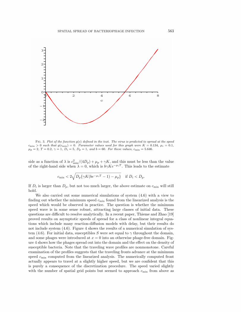
We define the function g(c) to be the left-hand side minus the right-hand side ofthe second equation of (4.10), with λ∗ given by (4.12) and cmin replaced by c. Theresulting function is too complicated to write out explicitly but is easily handled inMAPLE. Of course, cmin solves g(cmin) = 0 and can easily be found either by readingoff the root from an accurate plot of g(c) or by using MAPLE commands for findingroots numerically. Figure 3 shows a plot of g(c) for typical parameter values (seecaption). We investigated how cmin depends on the values of all the parameters, andour main observations were as follows:

• If µi, µp, or T is increased, the result is a decrease in cmin.• If K, γ, b, Di, or Dp is increased, the result is an increase in cmin.• If the delay T is large, then the value of cmin is much more sensitive to Di than

to Dp. Presumably this is because virus particles with a host are transportedat the diffusivity of the infectives. To illustrate this, let T = 7 and otherparameters retain their Figure 3 values. Then cmin = 1.265. Keeping T = 7,if Di is then raised to 100, cmin rises to 5.623. But if instead Di = 5 and Dp

is raised to 100, then cmin rises only to 1.976.Analytical estimates for cmin can be obtained from other arguments, involving con-sideration of the graphs of the left- and right-hand sides of (4.9) as functions of λ.When c = cmin these two graphs just touch, at the value λ∗ just discussed. Considerfirst the case when Di < Dp (so the minimum of the right-hand side is to the right ofthe maximum of the left-hand side). In this situation the maximum of the left-hand

SPATIAL SPREAD OF BACTERIOPHAGE INFECTION 563

2

0

-2

3

1

-1

c

8640 2

Fig. 3. Plot of the function g(c) defined in the text. The virus is predicted to spread at the speedcmin > 0 such that g(cmin) = 0. Parameter values used for this graph were K = 0.134, µi = 0.1,µp = 2, T = 0.2, γ = 1, Di = 5, Dp = 1, and b = 60. For these values, cmin = 5.646.

side as a function of λ is c2min/(4Dp) + µp + γK, and this must be less than the valueof the right-hand side when λ = 0, which is bγKe−µiT . This leads to the estimate

cmin < 2√Dp{γK(be−µiT − 1) − µp} if Di < Dp.

If Di is larger than Dp, but not too much larger, the above estimate on cmin will stillhold.

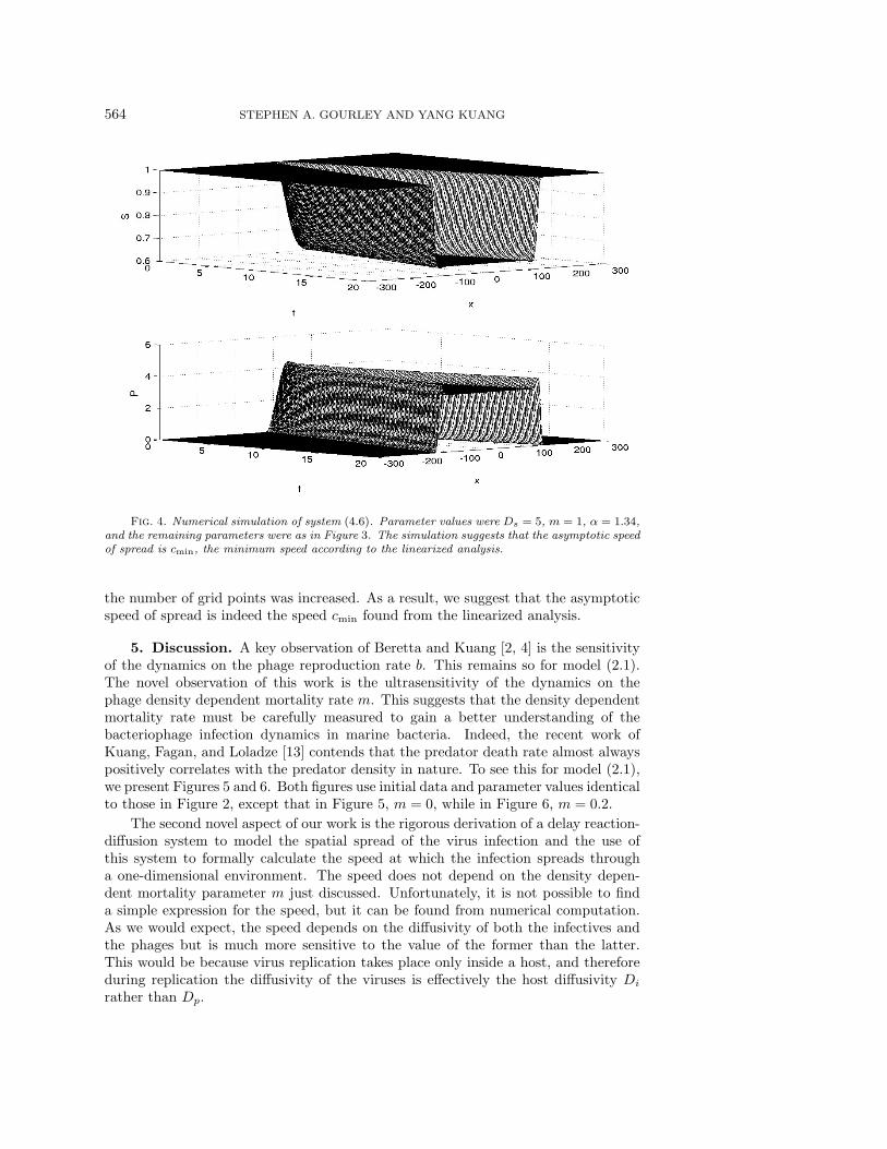
We also carried out some numerical simulations of system (4.6) with a view tofinding out whether the minimum speed cmin found from the linearized analysis is thespeed which would be observed in practice. The question is whether the minimumspeed wave is in some sense robust, attracting large classes of initial data. Thesequestions are difficult to resolve analytically. In a recent paper, Thieme and Zhao [19]proved results on asymptotic speeds of spread for a class of nonlinear integral equa-tions which include many reaction-diffusion models with delay, but their results donot include system (4.6). Figure 4 shows the results of a numerical simulation of sys-tem (4.6). For initial data, susceptibles S were set equal to γ throughout the domain,and some phages were introduced at x = 0 into an otherwise phage-free domain. Fig-ure 4 shows how the phages spread out into the domain and the effect on the density ofsusceptible bacteria. Note that the traveling wave profiles are nonmonotone. Carefulexamination of the profiles suggests that the traveling fronts advance at the minimumspeed cmin computed from the linearized analysis. The numerically computed frontactually appears to travel at a slightly higher speed, but we are confident that thisis purely a consequence of the discretization procedure. The speed varied slightlywith the number of spatial grid points but seemed to approach cmin from above as

564 STEPHEN A. GOURLEY AND YANG KUANG

Fig. 4. Numerical simulation of system (4.6). Parameter values were Ds = 5, m = 1, α = 1.34,and the remaining parameters were as in Figure 3. The simulation suggests that the asymptotic speedof spread is cmin, the minimum speed according to the linearized analysis.

the number of grid points was increased. As a result, we suggest that the asymptoticspeed of spread is indeed the speed cmin found from the linearized analysis.

5. Discussion. A key observation of Beretta and Kuang [2, 4] is the sensitivityof the dynamics on the phage reproduction rate b. This remains so for model (2.1).The novel observation of this work is the ultrasensitivity of the dynamics on thephage density dependent mortality rate m. This suggests that the density dependentmortality rate must be carefully measured to gain a better understanding of thebacteriophage infection dynamics in marine bacteria. Indeed, the recent work ofKuang, Fagan, and Loladze [13] contends that the predator death rate almost alwayspositively correlates with the predator density in nature. To see this for model (2.1),we present Figures 5 and 6. Both figures use initial data and parameter values identicalto those in Figure 2, except that in Figure 5, m = 0, while in Figure 6, m = 0.2.

The second novel aspect of our work is the rigorous derivation of a delay reaction-diffusion system to model the spatial spread of the virus infection and the use ofthis system to formally calculate the speed at which the infection spreads througha one-dimensional environment. The speed does not depend on the density depen-dent mortality parameter m just discussed. Unfortunately, it is not possible to finda simple expression for the speed, but it can be found from numerical computation.As we would expect, the speed depends on the diffusivity of both the infectives andthe phages but is much more sensitive to the value of the former than the latter.This would be because virus replication takes place only inside a host, and thereforeduring replication the diffusivity of the viruses is effectively the host diffusivity Di

rather than Dp.

SPATIAL SPREAD OF BACTERIOPHAGE INFECTION 565

0 5 10 15 200

5

10

15

20τ=0.01

s, p

sp

0 5 10 15 200

2

4

6

8

10

12

14τ=0.2

s, p

sp

0 10 20 300

2

4

6

8

10

12τ=0.3

time t

s, p

sp

0 10 20 300

0.5

1

1.5τ=1.1

time t

s, p

sp

Fig. 5. A solution of model (3.16) with s(θ) = 0.3, p(θ) = 1, θ ∈ [−τ, 0], where µp = 14.925,b = 75, µi = 1.5, α = 10, m = 0, and τ varies from 0.01 to 1.1.

0 5 10 15 200

5

10

15

20τ=0.01

s, p

sp

0 5 10 15 200

2

4

6

8

10

12

14τ=0.2

s, p

sp

0 10 20 300

2

4

6

8

10

12τ=0.3

time t

s, p

sp

0 10 20 300

0.5

1

1.5τ=1.1

time t

s, p

sp

Fig. 6. A solution of model (3.16) with s(θ) = 0.3, p(θ) = 1, θ ∈ [−τ, 0], where µp = 14.925,b = 75, µi = 1.5, α = 10, m = 0.2, and τ varies from 0.01 to 1.1.

566 STEPHEN A. GOURLEY AND YANG KUANG

Acknowledgment. We would like to thank Zdzislaw Jackiewicz of Arizona StateUniversity for help with the numerical simulation of the reaction-diffusion model.

REFERENCES

[1] E. Beltrami and T. O. Carroll, Modeling the role of viral disease in recurrent phytoplanktonblooms, J. Math. Biol., 32 (1994), pp. 857–863.

[2] E. Beretta and Y. Kuang, Modeling and analysis of a marine bacteriophage infection, Math.Biosci., 149 (1998), pp. 57–76.

[3] E. Beretta, M. Carletti, and F. Solimano, On the effects of environmental fluctuations ina simple model of bacteria-bacteriophage infection, Canad. Appl. Math. Quart., 8 (2000),pp. 321–366.

[4] E. Beretta and Y. Kuang, Modeling and analysis of a marine bacteriophage infection withlatency period, Nonlinear Anal. Real World Appl., 2 (2001), pp. 35–74.

[5] E. Beretta and Y. Kuang, Geometric stability switch criteria in delay differential systemswith delay dependent parameters, SIAM. J. Math. Anal., 33 (2002), pp. 1144–1165.

[6] O. Bergh, K.Y. Borsheim, G. Bratbak, and M. Heldal, High abundance of viruses foundin aquatic environments, Nature, 340 (1989), pp. 467–468.

[7] B. J. M. Bohannan and R. E. Lenski, Linking genetic change to community evolution: In-sights from studies of bacteria and bacteriophage, Ecology Letters, 3 (2000), pp. 362–377.

[8] A. Campbell, Conditions for the existence of bacteriophage, Evolution, 15 (1961), pp. 153–165.[9] M. Carletti, Numerical determination of the instability region for a delay model of phage-

bacteria interaction, Numer. Algorithms, 28 (2001), pp. 27–44.[10] M. Carletti, On the stability properties of a stochastic model for phage-bacteria interaction

in open marine environment, Math. Biosci., 175 (2002), pp. 117–131.[11] S. A. Gourley, and J. W.-H. So, Extinction and wavefront propagation in a reaction-diffusion

model of a structured population with distributed maturation delay, Proc. Roy. Soc. Edin-burgh Sect. A, 133 (2003), pp. 527–548.

[12] Y. Kuang, Delay Differential Equations, with Applications in Population Dynamics, AcademicPress, Boston, 1993.

[13] Y. Kuang, W. F. Fagan, and I. Loladze, Biodiversity, habitat area, resource growth rateand interference competition, Bull. Math. Biol., 65 (2003), pp. 497–518.

[14] R. E. Lenski and B. R. Levin, Constraints on the coevolution of bacteria and virulent phage:A model, some experiments, and predictions for natural communities, Amer. Naturalist,125 (1985), pp. 585–602.

[15] J. D. Murray, Mathematical Biology, Springer-Verlag, Berlin, 1993.[16] L. M. Proctor and J. A. Fuhrman, Viral mortality of marine bacteria and cyanobacteria,

Nature, 343 (1990), pp. 60–62.[17] H. L. Smith, A structured population model and a related functional-differential equation:

Global attractors and uniform persistence, J. Dynam. Differential Equations, 6 (1994),pp. 71–99.

[18] J. W.-H. So, J. Wu, and X. Zou, A reaction-diffusion model for a single species with agestructure. I. Travelling wavefronts on unbounded domains, Proc. Roy. Soc. London Ser. A,457 (2001), pp. 1841–1853.

[19] H. R. Thieme and X.-Q. Zhao, Asymptotic speeds of spread and traveling waves for inte-gral equations and delayed reaction-diffusion models, J. Differential Equations, 195 (2003),pp. 430–470.

[20] G. S. K. Wolkowicz, H. Xia, and J. Wu, Global dynamics of a chemostat competition modelwith distributed delay, J. Math. Biol., 38 (1999), pp. 285–316.

[21] J. Wu and X. Zou, Travelling wave fronts of reaction-diffusion systems with delay, J. Dynam.Differential Equations, 13 (2001), pp. 651–687.