A Design Space and its Patterns: Modelling 2phase Asynchronous Pipelines Graham Birtwistle 1 and Kenneth S. Stevens 2 1 Sheffield University, Yorkshire, UK [email protected]2 University of Utah, Salt Lake City, USA [email protected]Abstract We present a systematic way of studying state machine based design spaces and apply it to the study of asynchronous pipelines. Starting with the specification of the most concurrent behaviour as a state machine, all possible valid smaller designs may be generated by systematically removing structured patterns of output states (L cuts) and input states (R cuts). Taking the cartesian product of cuts L×R yields the complete design space which may then be partitioned according to well understood design styles. In this paper we extend previous results by studying mixed asynchronous pipelines of which homogeneous behaviours form a subset. The approach is presented using the much smaller 2phase setting (3×6) but the insights and structures revealed carry over to full 4phase designs (35×140). We present a complete overview of mixed 2phase linear pipeline behaviours; show how their structuring L cuts and R cuts relate; characterise the behaviours of linear pipelines in terms of these cuts for any depth; and show how the much larger R mixed behaviour patterns can be calculated from knowledge of the L behaviour patterns. Applications of the theory cover mixed linear pipeline and ring behaviours and the automatic generation of quality circuits from our specifications. 1 Setting and approach This work arose from our long standing interest in designing, specifying and building asyn- chronous microprocessors [2, 4, 5, 7, 21, 38, 39]. In the first stage of design development, our practice is to concentrate solely upon control signals and the ways in which they can interleave. This enables us to check that each subsystem and its compositions work together harmoniously (are live, deadlock free, preserve essential cyclic properties, ...) before extending the model towards data movements and calculations. The computational core of a microprocessor lies in its pipelined datapath. (At the control signal level, combinational circuits minimise down and can be considered mere delays.) When we experimented with structured pipelines of differing widths and depths, they minimised down to an observationally equivalent linear pipeline structure of the same depth, but usually one not composed from the controller used in its design. This aroused our curiosity. Our notation of choice has been CCS, Milner’s Calculus of Communicating Systems [1, 32]. CCS is a system description language based upon communicating agents (state machines). Mil- ner noticed that concurrent processes have an algebraic structure: given processes P and Q, we can construct new processes combining P and Q sequentially (example in Section 2.2) or in parallel (example in Section 2.3). The resulting composition will be a new process (in our case, system of circuits) whose behaviour depends upon those of P and of Q and of their com- bining operator. Further CCS provides just one inter-process communication mechanism which corresponds directly to the asynchronous circuit handshake. CCS has a number of pertinent at- tributes: it models arbitrary delays and interleaving behaviours which makes it straightforward to capture the signal level behaviour of asynchronous circuits and systems; and it has a simple and well understood formal semantics to support reasoning about designs, their properties, 34 A. Voronkov, M. Korovina (eds.), HOWARD-60, pp. 34–
Transcript
A Design Space and its Patterns:Modelling 2phase Asynchronous Pipelines
We present a systematic way of studying state machine based design spaces and applyit to the study of asynchronous pipelines. Starting with the specification of the mostconcurrent behaviour as a state machine, all possible valid smaller designs may be generatedby systematically removing structured patterns of output states (L cuts) and input states(R cuts). Taking the cartesian product of cuts L×R yields the complete design spacewhich may then be partitioned according to well understood design styles. In this paper weextend previous results by studying mixed asynchronous pipelines of which homogeneousbehaviours form a subset. The approach is presented using the much smaller 2phase setting(3×6) but the insights and structures revealed carry over to full 4phase designs (35×140).We present a complete overview of mixed 2phase linear pipeline behaviours; show howtheir structuring L cuts and R cuts relate; characterise the behaviours of linear pipelinesin terms of these cuts for any depth; and show how the much larger R mixed behaviourpatterns can be calculated from knowledge of the L behaviour patterns. Applications ofthe theory cover mixed linear pipeline and ring behaviours and the automatic generationof quality circuits from our specifications.
1 Setting and approach
This work arose from our long standing interest in designing, specifying and building asyn-chronous microprocessors [2, 4, 5, 7, 21, 38, 39]. In the first stage of design development, ourpractice is to concentrate solely upon control signals and the ways in which they can interleave.This enables us to check that each subsystem and its compositions work together harmoniously(are live, deadlock free, preserve essential cyclic properties, ...) before extending the modeltowards data movements and calculations.
The computational core of a microprocessor lies in its pipelined datapath. (At the controlsignal level, combinational circuits minimise down and can be considered mere delays.) Whenwe experimented with structured pipelines of differing widths and depths, they minimised downto an observationally equivalent linear pipeline structure of the same depth, but usually onenot composed from the controller used in its design. This aroused our curiosity.
Our notation of choice has been CCS, Milner’s Calculus of Communicating Systems [1, 32].CCS is a system description language based upon communicating agents (state machines). Mil-ner noticed that concurrent processes have an algebraic structure: given processes P and Q,we can construct new processes combining P and Q sequentially (example in Section 2.2) orin parallel (example in Section 2.3). The resulting composition will be a new process (in ourcase, system of circuits) whose behaviour depends upon those of P and of Q and of their com-bining operator. Further CCS provides just one inter-process communication mechanism whichcorresponds directly to the asynchronous circuit handshake. CCS has a number of pertinent at-tributes: it models arbitrary delays and interleaving behaviours which makes it straightforwardto capture the signal level behaviour of asynchronous circuits and systems; and it has a simpleand well understood formal semantics to support reasoning about designs, their properties,
34 A. Voronkov, M. Korovina (eds.), HOWARD-60, pp. 34–
A Design Space and its Patterns Birtwistle, Stevens
and their equivalences. Additionally CCS has a reliable public domain tool support, the CWB(Concurrency Workbench [33]), with built-in minimisation to the smallest equivalent state ma-chine and an implementation of the very powerful modal-µ property checking language—seeStirling’s sterling account [41, Chapter 6, pages 141-153].
1.1 Previous Work and its Approach
Our previous work [6, 8, 34] has been concerned with mainly 4phase asynchronous homogeneouslinear and structured parallel pipelines. The asynchronous community has made great effortsto present circuits clearly [9, 14, 16, 18, 19, 22, 23, 24, 25, 26, 27, 35, 36, 42, 44, 46]. This bodyof work enabled us to model real practical designs rather than experiment with a few idealisedones and kept us grounded. Importantly, the corpus was large to guide our research directions.Initial Survey. It is common practice within the community to specify designs graphically(STG [13, 37, 45]) or algebraically (CSP [11, 12, 26, 28, 29, 30, 31]) at the signal level—ourchosen level of abstraction. Some forty published 4phase designs were translated from their orig-inal presentations into CCS. STG specifications include internal state variables which assist thefavoured CAD tool Petrify [15] to target a specific implementation by delaying outgoing signalsuntil an internal state has been reached. We first mapped all these signals into CCS and then,by simply hiding any explicit mention of an STG internal variable name, retained its inherentconstraints as extra arbitrary length internal delays. In this way, our CCS model characterizesthe signal interleaving possibilities relevant to pipelining. To emphasize this distinction, wecall our minimised CCS state machine descriptions shapes. Shapes operate at the same level ofabstraction as STGs and our specifications lead directly to circuits in silicon [34]. Brunvand,Lines and Martin have used CSP equally abstractly to generate silicon [12, 26, 31, 44].Generalisation. The forty 4phase designs surveyed in the published literature gave rise tojust 18 distinct shapes. Since the behaviour of each and every shape is expressed solely in termsof external control signals, shape behaviours could then be compared, contrasted, and ordered.From comparison of these shapes, we noted a mathematically ideal shape, max 1, from whichall published designs could be defined by removing states. We claim that max 1 is the mostconcurrent possible shape. In support of this claim, the union of published shapes is preciselymax 1. This led to generating all possible subshapes by systematically cutting away states frommax 1. This is easiest to carry out in an algebraic notation—hence the aptness of CCS.
1.2 Intuition: MAX and its cutaways.
Consider the FSM MAX shown at the top of Figure 1. MAX has 20 states arranged in 5 rowsand 4 columns. The initial state is marked START and the terminal state DONE. Informally,the protocol is to take us from the start state to the done state by making only forward → ordownward ↓ moves. To save clutter we have omitted arrowheads and labels: horizontal arcs run
MAXSTART
DONECol cut: L321
321
Shape: L321.R2100
Row cut: R2100
2100
Figure 1: MAX and its cutaways
35
A Design Space and its Patterns Birtwistle, Stevens
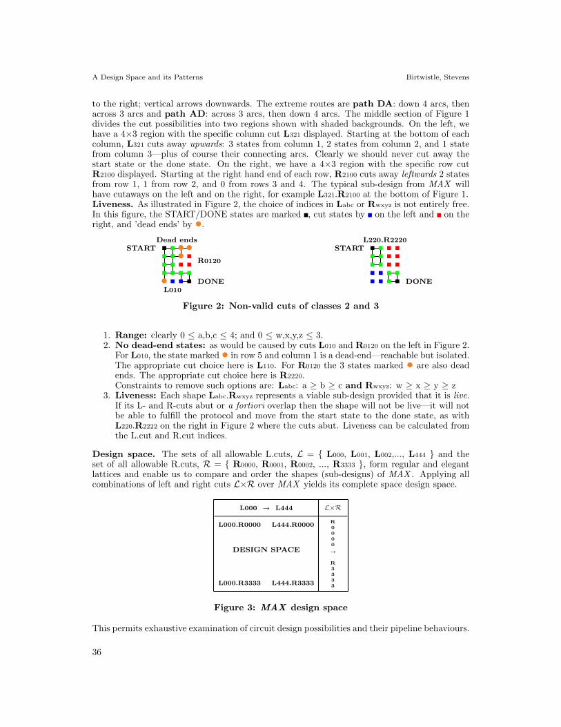
to the right; vertical arrows downwards. The extreme routes are path DA: down 4 arcs, thenacross 3 arcs and path AD: across 3 arcs, then down 4 arcs. The middle section of Figure 1divides the cut possibilities into two regions shown with shaded backgrounds. On the left, wehave a 4×3 region with the specific column cut L321 displayed. Starting at the bottom of eachcolumn, L321 cuts away upwards: 3 states from column 1, 2 states from column 2, and 1 statefrom column 3—plus of course their connecting arcs. Clearly we should never cut away thestart state or the done state. On the right, we have a 4×3 region with the specific row cutR2100 displayed. Starting at the right hand end of each row, R2100 cuts away leftwards 2 statesfrom row 1, 1 from row 2, and 0 from rows 3 and 4. The typical sub-design from MAX willhave cutaways on the left and on the right, for example L321.R2100 at the bottom of Figure 1.Liveness. As illustrated in Figure 2, the choice of indices in Labc or Rwxyz is not entirely free.In this figure, the START/DONE states are marked , cut states by on the left and on theright, and ’dead ends’ by •.
L010
Dead endsSTART
DONE•R0120
••• START
DONE
L220.R2220
Figure 2: Non-valid cuts of classes 2 and 3
1. Range: clearly 0 ≤ a,b,c ≤ 4; and 0 ≤ w,x,y,z ≤ 3.2. No dead-end states: as would be caused by cuts L010 and R0120 on the left in Figure 2.
For L010, the state marked • in row 5 and column 1 is a dead-end—reachable but isolated.The appropriate cut choice here is L110. For R0120 the 3 states marked • are also deadends. The appropriate cut choice here is R2220.Constraints to remove such options are: Labc: a ≥ b ≥ c and Rwxyz: w ≥ x ≥ y ≥ z
3. Liveness: Each shape Labc.Rwxyz represents a viable sub-design provided that it is live.If its L- and R-cuts abut or a fortiori overlap then the shape will not be live—it will notbe able to fulfill the protocol and move from the start state to the done state, as withL220.R2222 on the right in Figure 2 where the cuts abut. Liveness can be calculated fromthe L.cut and R.cut indices.
Design space. The sets of all allowable L.cuts, L = { L000, L001, L002,..., L444 } and theset of all allowable R.cuts, R = { R0000, R0001, R0002, ..., R3333 }, form regular and elegantlattices and enable us to compare and order the shapes (sub-designs) of MAX . Applying allcombinations of left and right cuts L×R over MAX yields its complete space design space.
L×RL000 → L444
DESIGN SPACE
R0000
→
R3333
L000.R0000
L000.R3333
L444.R0000
L444.R3333
Figure 3: MAX design space
This permits exhaustive examination of circuit design possibilities and their pipeline behaviours.
36
A Design Space and its Patterns Birtwistle, Stevens
1.3 Contributions
In this paper we apply these ideas to studying and predicting the behaviours of mixed pipelines.Homogeneous results drop out as a subset in this study. Mixed pipelines enjoy a huge increasein variety over homogeneous pipelines, but this very generality has uncovered unifying resultswith practical applications. In particular, our previous R.cut sets [8, 34] are closed undercomposition for homogeneous pipelines, but not for mixed. A simple modification has led totwo key discoveries:
1. A unique notation for pipelines of any depth in terms of the closed set of shape cutaways.
2. The relation between the L.cut set and the R.cut set. We already had a neat lattice forL.cuts as a planar wedge. We can now restructure the closed R.cuts into (2 for 2phase, 4for 4phase) related planar wedges each of which is isomorphic to the L wedge. This hasa practical application when we come to predict pipeline behaviours, since experimentsshow that if we know how a L.cut behaves we can calculate how a related R.cut behaves.
The full 4phase design space has 35 L.cuts and 140 R.cuts; its untimed sub-space (delay in-sensitive and speed independent shapes only) has 10 L.cuts and 20 R.cuts. Evaluating theirdesign spaces for just pipelines of depth 2 would entail 24.01 million and 160 thousand experi-ments respectively as against just 324 for 2phase. Accordingly we present exhaustive practicalresults for the 3×6 2phase design style. Work in progress confirms that our 2phase insights andstructures carry over into the above 4phase design spaces (see example in Section 5.4).
1.4 Structure of the paper
In the remaining sections in this paper: Section 2 introduce the CCS notation via examplesleading to the model of data transmission which underlies pipeline behaviours. Section 3 ex-plains the design and implementation of Furber’s classic 2phase pipeline stage (which we callmax 1) using simple building blocks expressed in CCS. It also covers pipeline models constructedfrom max 1 and discusses their specification. Section 4 covers the structure of cuts, their lat-tices, how they are related, and how they define the family of subdesigns from max 1. Section 5presents new results on mixed pipelines, uses lattices to uncover their pipeline structures andpipelined behaviours; and predicts the behaviours of mixed pipelines and rings. Section 6 givesapplications to circuit design. Section 7 is an overview and summary.
2 CCS as a System Description Language
CCS describes objects (agents, circuits, processes) by defining the states they can occupy andthe actions that cause them to move from state and to another state or back to the same state.In this section we give an introduction to defining individual objects in CCS, how objectscommunicate via handshakes, and give a simple model of 2phase bundled data transmissionprotocol as a lead in to asynchronous modelling.
2.1 Individual objects
0: The simplest object in CCS is 0 which can do nothing; it cannot receive or send signals, norhas it any local actions. It is said to be deadlocked.Prefixing: Sequential objects can be built from 0 by prefixing actions which are executed inorder. For example, Match1 = strike.burn.0 describes an object that be struck, then burns,whereupon it deadlocks (is spent). The separating dot . indicates an arbitrary delay and maybe read as then some time later. Except for the deadlocked state, 0, states always start with
37
A Design Space and its Patterns Birtwistle, Stevens
upper case letters, e.g. Match1 . Actions always start with lower case letters. We distinguishbetween input actions (e.g. strike) and output actions (e.g. burn) which are over-barred.Choice: Not all objects are sequential. Many have choices of action stream. For example,Match2 = strike.(burn.0 + fail.Match2 + dead.0) describes a match that after being struck has3 distinct behavioural options: it may burn and become spent or it may fail to light whereuponit may choose to repeat the action repertoire from the beginning, or (perhaps the match headhas dropped off) is thrown away.
Match1
0
?
?
strike
burn
Match2
0
? 6
? ?
strike fail
burn dead
Figure 4: State machines for Match1 and Match2
Figure 4 shows state machine descriptions of the linear Match1 and the cyclic Match2 . Noticethe tight correspondences with their CCS specifications. We have made fail and dead local traceactions. Trace variables are useful documentation aids at key points and can be invaluablewhen property checking. We always show them in serif font.
2.2 Sequential Composition
Suppose we are given two objects, FST and SND , each of which upon receiving a request,carries out a local task, emits an acknowledgement and is then ready to repeat its cycle. Wewish to allow FST and SND to cooperate in series: having completed a task1, FST hands overfor SND to finish off by carrying out a task2. This communication is arranged by connectingthe output acknowledgement of FST to the input request of SND as in Figure 5.
FST = rF .task1.aF .FST SND = rS .task2.aS .SND
FST SNDhs
rF hs hs aS
Figure 5: FS : handshake communication
For two objects to communicate via a direct handshake they must:
1. Agree on a common name for their communication line, here hs
2. Rename the sender’s action to match the line name, that is in FST aF → hs
3. Rename the receiver’s action to match the line name, that is in SND rS → hs
Table 1 defines FS as the parallel composition of FST and SND . It first lists the constituentobjects, parenthesised and with separator |, here (FST | SND); followed by its curly bracketedhandshake lines (in general they are separated by commas, but here) \ { hs }. This specificationhas been embellished by m arrows. They are not part of formal CCS—here they highlight thehandshake.
38
A Design Space and its Patterns Birtwistle, Stevens
FST = rF . task1 . hs . FSTm
SND = hs . task2 . aS . SND
FS = ( FST | SND ) \ { hs }
Table 1: Specification of FS
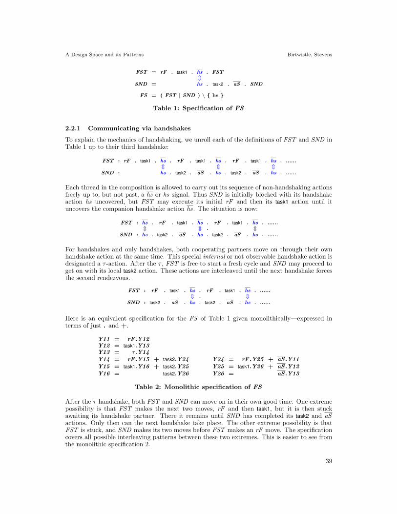
2.2.1 Communicating via handshakes
To explain the mechanics of handshaking, we unroll each of the definitions of FST and SND inTable 1 up to their third handshake:
SND : hs . task2 . aS . hs . task2 . aS . hs . ......
Each thread in the composition is allowed to carry out its sequence of non-handshaking actionsfreely up to, but not past, a hs or hs signal. Thus SND is initially blocked with its handshakeaction hs uncovered, but FST may execute its initial rF and then its task1 action until ituncovers the companion handshake action hs. The situation is now:
FST : hs . rF . task1 . hs . rF . task1 . hs . ......m m . m
SND : hs . task2 . aS . hs . task2 . aS . hs . ......
For handshakes and only handshakes, both cooperating partners move on through their ownhandshake action at the same time. This special internal or not-observable handshake action isdesignated a τ -action. After the τ , FST is free to start a fresh cycle and SND may proceed toget on with its local task2 action. These actions are interleaved until the next handshake forcesthe second rendezvous.
After the τ handshake, both FST and SND can move on in their own good time. One extremepossibility is that FST makes the next two moves, rF and then task1, but it is then stuckawaiting its handshake partner. There it remains until SND has completed its task2 and aSactions. Only then can the next handshake take place. The other extreme possibility is thatFST is stuck, and SND makes its two moves before FST makes an rF move. The specificationcovers all possible interleaving patterns between these two extremes. This is easier to see fromthe monolithic specification 2.
39
A Design Space and its Patterns Birtwistle, Stevens
2.2.2 Minimisation
The state diagram for a minimised specification of FS is:
�� �� �� �� �� �� �� �� �� ���� �� �� �� �� ��
task2 task2 task2
? ? ?
��
� �?
��
� �?
��
� �?
aS
- - - -rF rFtask1 task1
- -rF task1
Figure 6: State graph of minimised FS
This is the smallest (in state size) definition of FS which is observably equivalent to the specifica-tion given in Table 1. Compared with the monolithic specification in Table 2, the non-observableτ action is deleted. The definition of state Y13 is deleted and remaining references to it areupdated to Y14 .
Coda. For all but the simplest machines, it usually pays to define an object in terms ofits interfaces (as we did here with FST and SND) and then constrain them. This composedspecification will be the easiest to reason about, and once satisfied, the CWB will produce itsminimised form automatically.
We have now given all the syntax and (informal) semantics for CCS that we need: theoperators . + |, hiding, and handshaking. This enables us to deal with asynchronous hardwarecommunication signals in appropriate detail. As with all state machine based descriptions,incorporating data would, of course, entail an exponential growth in state size.
2.3 2phase Bundled Data Transmission
We now present a simple model consisting of an output O and an input I cooperating via the2phase protocol. It forms the core of how data gets transmitted down an asynchronous pipeline(see next section) and is an important first step in understanding the much used 2phase bundleddata protocol.
O I
r
a
-
�
r
a
r
a
Figure 7: Transmitting bundled data between processes
Suppose that O and I are connected by a bus down which data values are transmitted insequence from O to I . r/a are request/acknowledge communication wires respectively whichensure the safety of each transmission. Once O has loaded the next data value onto the bus, itsends a signal on line r . On receipt of which, I understands that a fresh data value is availableand copies it locally from the bus. Once this data capture is complete, I signals on a to informO that it can start the next transaction and safely overwrite the bus with the next data value.Using pD and gD as trace variables, the CCS description of this system is:
40
A Design Space and its Patterns Birtwistle, Stevens
O = pD . r . a . OI = r . gD . a . I
OI = ( O | I ) \ { r , a }
Table 3: Specification of OI
Commentary on Table 3
pD: O puts fresh data on the bus linking O to I .r⇔r : When the data is stable, O sends a request signal on communication line r to I . O now
passively awaits an acknowledgement from I .gD: On receipt of the request signal on r , I reads the data from the bus.a⇔a: Once the data is captured, I sends an acknowledgement signal on line a back to O and
passively awaits the next request
On receipt of a, O knows that the current data value has been safely passed to I . O maynow actively prepare the next data value and place it on the bus. In Table 4 we unroll thespecification of SR through the specific transaction.
Transaction 1 • Transaction 2 •
O = pD . r↑ . a↑ • pD . r↓ . a↓ • ....m m m m
I = r↑ . gD . a↑ • r↓ . gD . a↓ • ....
Table 4: Unrolling the specification of OI through 2 iterations
It is easy to show formally that OI is observationally equivalent to both specifications below:
OI2 = pD . τ . gD . τ . OI2
OI3 = pD . gD . OI3
which confirm that pD and gD alternate. Reading ≺ as precedes, pDk ≺ gDk means that I alwaysreads fresh data; gDk ≺ pDk+1 means that O cannot overwrite unread data. So the protocol isdata independent and safe. As a final remark, transaction phases are identical in the 2phaseprotocol, so there is no need to indicate parity by ↑ and ↓.
2.3.1 4phase Protocol
In the equivalent 4phase version of this protocol, each signal goes up and down once per trans-action. Hence its alternative name: Return To Zero, or RTZ.
Transaction 1 •
O = pD1 . r↑ . a↑ . r↓ . a↓ • ....m m m m
I = r↑ . gD1 . a↑ . r↓ . a↓ • ....
At first sight this seems a waste of energy and time compared to 2phase. But 4phase hardwarecircuits may be simpler than 2phase and the down phase of one transaction may overlap withthe up phase of its successor. The increased variety presents greater opportunities and greaterchallenges for engineers. It also gives rise to surprisingly larger design spaces.
41
A Design Space and its Patterns Birtwistle, Stevens
2.4 Aptness of CCS for Circuits at the Control Signal Level
In later sections we will apply our algebraic approach to specifying the compositional propertiesof both homogeneous and mixed linear asynchronous pipeline and ring structures. We willexplain how to describe basic asynchronous circuits as objects (state machines), the standardhandshake method of synchronising circuits, how to compose cooperating circuits into systems,all the while using the 2phase design communication protocol and modelling in CCS. Whichbegs the question ‘How well does CCS capture asynchronous hardware?’.
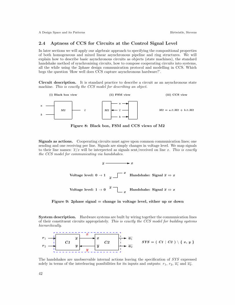
Circuit description. It is standard practice to describe a circuit as an asynchronous statemachine. This is exactly the CCS model for describing an object.
(i) Black box view (ii) FSM view (iii) CCS view
M2
a
b
c M2
-
-
�
a
b
c M2 = a.c.M2 + b.c.M2
Figure 8: Black box, FSM and CCS views of M2
Signals as actions. Cooperating circuits must agree upon common communication lines; onesending and one receiving per line. Signals are simply changes in voltage level. We map signalsto their line names: x/x will be interpreted as signals sent/received on line x . This is exactlythe CCS model for communicating via handshakes.
x - x
x
x
x
x
Voltage level: 0 → 1
Voltage level: 1 → 0
Handshake: Signal x ⇔ x
Handshake: Signal x ⇔ x
Figure 9: 2phase signal = change in voltage level, either up or down
System description. Hardware systems are built by wiring together the communication linesof their constituent circuits appropriately. This is exactly the CCS model for building systemshierarchically.
C1 C2
x
y
-
-
-
-
r1
r2
a1
a2
-
�
x
y
x
ySYS = ( C1 | C2 ) \ { x , y }
The handshakes are unobservable internal actions leaving the specification of SYS expressedsolely in terms of the interleaving possibilities for its inputs and outputs: r1, r2, a1 and a2.
42
A Design Space and its Patterns Birtwistle, Stevens
2phase protocol. In asynchronous systems, there are no coordinating clocks. In 2phasedesign, each circuit is passive until awoken by a request signal (or possibly several). When ithas finished its current task, it will send a completion signal (or possibly several) and then fallpassive again awaiting its next request. This is modelled in CCS using the req/ack protocol asin the 2phase data transmission example of Section 2.3.
3 Modelling asynchronous pipelines in CCS
In this section we describe Furber’s classic implementation of a 2phase pipeline stage [20] anduse this description to specify a suitable abstraction in CCS. Under common assumptions, weargue that this is the most concurrent behaviour achievable. We then recount experiments withthis stage when pipelined and report their resulting structures and patterns. These patternsform the basis for specifying pipelines in the next sections.
STAGE
LATCH
CONTROLLER
dIN dOUT
6?
rL aL
-
�
-
�
ir
ia
or
oa
Figure 10: Latch and Controller interplay
The basic pipeline building block is the stage which is the composition of a latch and itscontroller as shown in Figure 10. The latch has two safe states: open in which it will admit thefresh data value pending on dIN and closed when it holds its current value steady both internallyand on dOUT . The controller is responsible for the safety of the open and close operations.Signal lines ir/ia enable Input request/acknowledge communication with a source on the left;signal lines or/oa enable Output request/acknowledge communication with a successor on theright. Linear pipelines are built by abutment with ork wired to irk+1, dOUT k to dIN k+1, andiak+1 to oak (see Figure 11).
ST1 ST2 ..... STk STk′
LPk ST
x
y
or
oa
ir
ia
or
oa
ir
ia
Figure 11: Building linear pipelines by abutment
43
A Design Space and its Patterns Birtwistle, Stevens
The construction of such linear pipelines has the straightforward recursive definition:
LP1(ir,ia,or,oa) = ST(ir,ia,or,oa)LPk+1(ir,ia,or,oa) = (LPk(ir,ia,x,y) | ST(x,y,or,oa)) \ { x , y }
with the request and acknowledge lines between LPk and LPk+1 being renamed x and yrespectively and hidden (syntactically \ { x , y }) in the definition of LPk+1 so that no othercircuit can access them.
3.1 Components for Building a Furber Stage
In this subsection we give signal level specifications of a latch and the basic circuits required tobuild a specific 2phase pipeline stage presented in Furber [20].
3.1.1 The Latch Model
The latch model in Figure 12 has an input bus dIN and output dOUT and two control linesrL and aL which allow it to be opened and closed.
rL = F
aL = F
CLOSEDdIN dOUT
rL = T
aL = T
OPENdIN dOUT
Figure 12: Open and closed latch states
There are two major latch disciplines: NC normally closed and NO normally open. In thisaccount, we follow the NC discipline only. Furber [20, section 3, page 221 et. seq.] providesclear descriptions of both protocols, their uses and their pitfalls.
When an NC latch is in its quiescent closed state, both rL and aL are low and bus dIN isdisconnected from the latch. We assume that the next data value to be captured, say Dk , hasbeen placed on the input bus dIN .
open: when rL is raised, dIN is connected to the latch. The data value on dIN , Dk , entersthe latch and is also copied onto dOUT . When these are both stable, the latch sends anacknowledgement to the controller by raising aL.
When the latch is open, rL = aL = T and dIN = latch = dOUT . Whilst open anyvariation in dIN will be passed through changing the value in the latch and on dOUT .
closed: when rL is lowered, dIN is disconnected from the latch. The data value is now saidto be captured. The latch then sends an acknowledgement signal informing the controllerthat the latch is closed by lowering aL.
When the latch is closed, rL = aL = F, latch = dOUT and will not be affected by anychange on dIN .
Note that data is guaranteed stable in the latch and on dOUT only when the latch is closed.Since we map signals to wires, the specification of NC (with trace variables) is simply:
NC = rL.open.aL.rL.closed.aL.NC
State machines are quite smart at figuring out whether a signal is to go up or down.
44
A Design Space and its Patterns Birtwistle, Stevens
3.1.2 Common 2phase Building Blocks
a T2r b
c
T2 = a .b.a .c.T2
a
bM2 c
M2 = a .c.M + b.c.M2
a F2
b
c
F2 = a .(b.c.F2 + c.b.F2 )
a
bC2 c
C2 = a .b.c.C2 + b.a .c.C2
Figure 13: T2/M2 and F2/C2 circuit descriptions
Toggle: T2 = a.b.a.c.T2 The Toggle inputs a signal on a and routes it out on b. Onreceiving a second signal on a, it routes it out on c. Then this 4-cycle repeats. Thus oddnumbered input signals are routed out via b and even numbered input signals via c. It iscustomary to mark the first output line b of Toggle with a blob • in a circuit diagram.
Merge: M2 = a.c.M2 + b.c.M2 If a Merge receives its next input on a it will acknowledgeby emitting a signal on c. If it receives its next input on b it will also acknowledge byemitting a signal on c. The designer must see to it that the a.c and b.c transactions neveroverlap.
Fork: F2 = a.(b.c.F2 + c.b.F2) The F2 has one input a and two outputs b and c. Asignal arriving on a is routed to both b and c in turn but in either order. The F2 is usedto instigate 2 components running in parallel by firing up both.
Collector: C2 = a.b.c.C2 + b.a.c.C2 The C2 , commonly referred to as a C-element, hastwo inputs a and b and one output c. When signals have arrived on both its inputs, againin either order, it forwards an acknowledgement on c. The C2 element is used as acollector to ensure that the components in a 2-parallel system rendezvous. In general,input signals may be retracted, but as this will not occur in the implementation described,we use a simpler (sufficient) description of C2 .
3.1.3 FNC: Furber’s Normally Closed stage
FNC is constructed by wiring together a C2, an M2, a normally closed latch, a T2, and an F2fork as shown in Figure 14. For space reasons, the design is presented with the Input lines atthe top and the Output lines on the bottom. The C2 ensures that the previous data value has
C2
�� M2 Latch T2c s
ir
oa
ia
or
rL aL
dIN
dOUT
Figure 14: FNC: Furber’s normally closed latch
45
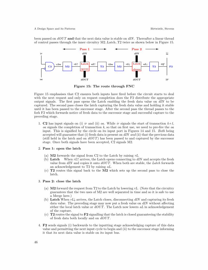
A Design Space and its Patterns Birtwistle, Stevens
been passed on dOUT and that the next data value is stable on dIN . Thereafter a linear threadof control passes through the inner circuitry M2..Latch..T2 twice as shown below in Figure 15.
c C2
��
Pass 1� - Pass 2� -
M2Latch
opensT2 M2
Latch
closesT2
ir
oa
ia
or
F2c2m rL↑ aL↑ t2m rL↓ aL↓ t2f
dIN
dOUT
dIN
dOUT
Figure 15: The route through FNC
Figure 15 emphasises that C2 ensures both inputs have fired before the circuit starts to dealwith the next request and only on request completion does the F2 distribute the appropriateoutput signals. The first pass opens the Latch enabling the fresh data value on dIN to becaptured. The second pass closes the latch capturing the fresh data value and holding it stableuntil it has been passed to the successor stage. After the second pass the thread passes to thefork F2 which forwards notice of fresh data to the successor stage and successful capture to thepreceding stage.
1. C2 has input signals on (i) ir and (ii) oa. While ir signals the start of transaction k+1,oa signals the completion of transaction k, so that on first use, we need to pre-fire the oainput. This is signified by the circle on its input port in Figures 14 and 15. Both beingaccepted will guarantee that (i) fresh data is present on dIN and (ii) that the previous data(still held in the latch and on dOUT ) has been passed to and captured by the successorstage. Once both signals have been accepted, C2 signals M2.
2. Pass 1: open the latch
(a) M2 forwards the signal from C2 to the Latch by raising rL.(b) Latch When rL↑ arrives, the Latch opens connecting to dIN and accepts the fresh
value from dIN and copies it onto dOUT . When both are stable, the Latch forwardsan acknowledgement to T2 by raising aL.
(c) T2 routes this signal back to the M2 which sets up the second pass to close thelatch.
3. Pass 2: close the latch
(a) M2 forward the request from T2 to the Latch by lowering rL. (Note that the circuitryguarantees that the two uses of M2 are well separated in time and so it is safe to usea Merge here.)
(b) Latch When rL↓ arrives, the Latch closes, disconnecting dIN and capturing its freshdata value. The preceding stage may now put a fresh value on dIN without affectingeither the local latch value or dOUT . The Latch now lowers aL in acknowledgementof the capture.
(c) T2 routes the signal to F2 signalling that the latch is closed guaranteeing the stabilityof fresh data both locally and on dOUT .
4. F2 sends signals (i) backwards to the inputting stage acknowledging capture of this datavalue and permitting the next input cycle to begin and (ii) to the successor stage informingit that its next data value is stable on its input bus.
46
A Design Space and its Patterns Birtwistle, Stevens
3.2 Specifying max 1
Figure 16 shows the two constituents of Furber’s pipeline stage: a normally closed latch and itsassociated controller.
NC
I | O
dIN dOUT
6
?rL aL
-
�
-
�ir
ia
or
oa
Figure 16: Latch and Controller interplay
Controller Initially we ignore trace variables and any interactions with the Latch. I definesthe cyclic sequence of actions on the incoming side and O describes the cyclic sequence ofactions on the outgoing side. Their separate descriptions follow the patterns established in OIin Section 2.3 but they cooperate ‘in reverse order’. The specification I = ir . ia . I is to beinterpreted as:
ir : when ready, the source places fresh data Dk on dIN and then signals its presence bysignalling on line ir . I is then blocked until certain that the previous datum Dk-1 hasbeen passed to the next stage.
ia: only when Dk has been captured may I return an acknowledgement to the source bysignalling on line ia.
I : whereupon the next input cycle begins
O , which acts as source for the next stage, gives the cycle of actions on the outgoing side: O =or . oa . O . To be safe, we will have to guarantee that O is blocked from emitting or until afresh data value has been captured by I . Our initial specification of a stage (without blocking)is just the composition of its input interface with its output interface:
I = ir . ia . IO = or . oa . OST = ( I | O )
Reading . as and some time later, we interpret their occurrences in ir .ia and oa.or as arbitraryinternal delays; and in ia.ir and or .oa as arbitrary external delays.
The blocking constraints between I and O are handled by two tokens which one may putor get . We use tokens NEXT with gN /pN and PASS with gP/pP operations1. The putter isnot delayed; the getter may be. The essential safety blockings are:
NEXT = gN .pN .NEXTPASS = pP.gP.PASS
I = ir . gP . ia . IO = gN . or . oa . O
ST = ( I | NEXT | PASS | O )
where gP will block I from capturing the next value until the current value has been passedthus preventing premature overwriting, and gN will block O from forwarding its or until a fresh
1I and O do not handshake directly but indirectly via NEXT and PASS . It saves on clutter if we put allthe over-barred handshake signals within the two tokens.
47
A Design Space and its Patterns Birtwistle, Stevens
value has been captured. All that remains is to free I by a judiciously placed pP and to free Oby a judiciously placed pN. The key to these synchronisations is:
I = ir . gP . capt . pN . ia . ir . gP . capt . pN . ia . ir . gP . .... I⇓ ⇑ ⇓ ⇑
O = gN . or . oa . pass . pP . gN . or . oa . pass . pP . .... O
in which we have temporarily included trace variables capt and pass for extra clarity. If we omitthe handshaking signals and retain only the traces and the get/put operations, we see thatthese synchronisations faithfully uphold safety by maintaining the cyclic ordering:
cycle ( gP ≺ capt ≺ pN ≺ gN ≺ pass ≺ pP )
( Controller | Latch interplay ) Our final step is to include the interactions with the latch.Taking a cue from the thread in Section 3.1.3, we choose to associate the latch open and closerequests with our thread I .
NC = rL . open . aL . rL . closed . aL . NCm m m m
I = ir . gP . rL . . aL . rL . . aL . pN . ia . I
O = gN . or . oa . pP . O
FNC = ( NC | I | NEXT | PASS | O ) \ { rL, aL, gN, pN, gP, pP }
Table 5: First specification of FNC
This is observationally equivalent to:
I = ir . gP . open . closed . pN . ia . I
O = gN . or . oa . pP . O
FNC = ( I | NEXT | PASS | O ) \ { gN, pN, gP, pP }
Dropping the trace variables which have served their purpose, we arrive at our final form of thespecification of an FNC stage:
I = ir . gP . pN . ia . I
O = gN . or . oa . pP . O
FNC = ( I | NEXT | PASS | O ) \ { gN, pN, gP, pP }
Table 6: Final specification of FNC
We claim that this specification is the least constrained since I is freed up (by pP/gP) as soonas O has received the acknowledgement oa confirming the current value has been successfullypassed downstream, and O is freed up (by pN/gN ) as soon as I has captured the next freshdata value. From now on, we will name it max 1.
Rider. Because open/close signals are entirely internal handshakes, the controller and thestage are observationally equivalent. For the same reason, normally open and normally closedvariations on the same controller have the same shape. See for example the 4 variations givenby Efthymiou and Garside in [19].
48
A Design Space and its Patterns Birtwistle, Stevens
�� �� �� �� �� �� �� �� �� ���� �� �� �� �� ��or or or
? ? ?
• ••
•
• •
•��
� �?
��
� �?
��
� �?
oa
- - - -ir iria ia
- -iria
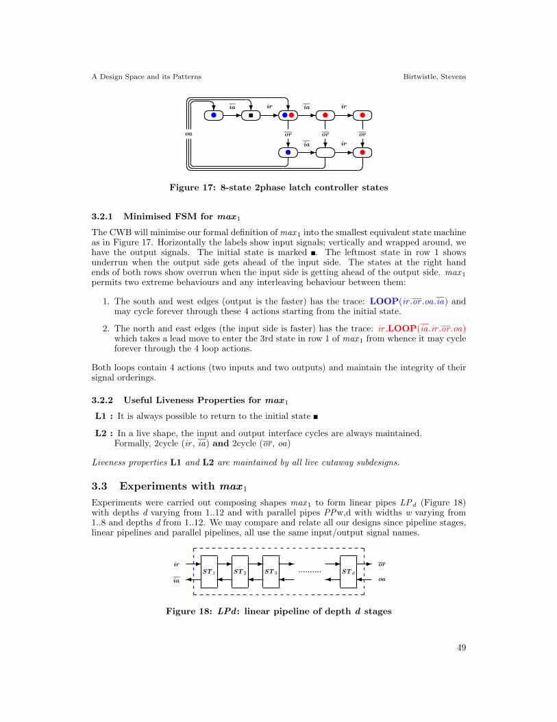
Figure 17: 8-state 2phase latch controller states
3.2.1 Minimised FSM for max 1
The CWB will minimise our formal definition of max 1 into the smallest equivalent state machineas in Figure 17. Horizontally the labels show input signals; vertically and wrapped around, wehave the output signals. The initial state is marked . The leftmost state in row 1 showsunderrun when the output side gets ahead of the input side. The states at the right handends of both rows show overrun when the input side is getting ahead of the output side. max 1
permits two extreme behaviours and any interleaving behaviour between them:
1. The south and west edges (output is the faster) has the trace: LOOP(ir .or .oa.ia) andmay cycle forever through these 4 actions starting from the initial state.
2. The north and east edges (the input side is faster) has the trace: ir .LOOP(ia.ir .or .oa)which takes a lead move to enter the 3rd state in row 1 of max 1 from whence it may cycleforever through the 4 loop actions.
Both loops contain 4 actions (two inputs and two outputs) and maintain the integrity of theirsignal orderings.
3.2.2 Useful Liveness Properties for max 1
L1 : It is always possible to return to the initial state
L2 : In a live shape, the input and output interface cycles are always maintained.Formally, 2cycle (ir , ia) and 2cycle (or , oa)
Liveness properties L1 and L2 are maintained by all live cutaway subdesigns.
3.3 Experiments with max 1
Experiments were carried out composing shapes max 1 to form linear pipes LPd (Figure 18)with depths d varying from 1..12 and with parallel pipes PPw,d with widths w varying from1..8 and depths d from 1..12. We may compare and relate all our designs since pipeline stages,linear pipelines and parallel pipelines, all use the same input/output signal names.
- - - - - -
������ST1 ST2 ST3 .......... STd
ir
ia
or
oa
Figure 18: LPd : linear pipeline of depth d stages
49
A Design Space and its Patterns Birtwistle, Stevens
3.3.1 MAX d: linear pipelines composed from max 1.
2phase pipelines constructed from max 1 stages grow in regular fashion with state sizes 8, 12,16, ... for pipes of length 1, 2, 3, ...
Figure 19: MAX 2: Linear pipeline built from two max 1 stages
Figure 19 shows the minimised state machine for depth 2 with the 4 extra states over max 1
inside a dashed box. As d increases, the shape (profile) of LPd remains the same: it increaseseach time by 2×2 states. This indicates full capacity: each stage added permits an extra datavalue to be stored.
Once the pattern of arrows in Figure 19 has been absorbed, a less cluttered picture of max 1
suffices which represents the initial state by and the other live states by •. This clutter freenotation is easy to extend to arbitrary pipelines:
With a little artistic license, we may indicate the shape of the pipeline MAX d built from dcopies of shape max 1 by
MAX 1 = max 1
MAX d+1 = MAX d ++••••
Table 8: Pipelines composed with max 1
3.3.2 PPw,d: parallel pipelines composed from MAX d
SPLIT2
LPd
LPd
JOIN2
- - - -
� �
- -
� � � �
ir
ia
or
oa
Figure 20: PP2,d: parallel pipeline of width 2 and depth d
The parallel pipeline shown in Figure 20 is composed from two inner linear pipes of thesame depth d . Entry and exit from the linear pipes is controlled by a SPLIT2 and a JOIN2
50
A Design Space and its Patterns Birtwistle, Stevens
respectively. The SPLIT2 ensures that on receiving a request on ir , appropriate data is fedto both inner pipes each of which will acknowledge when their own individual datum hasbeen captured. When both inner acknowledgements have been received, the SPLIT2 willacknowledge on ia. The JOIN2 works in analogous fashion. Thus each inner pipe will holdthe same number of data values but they progress independently. SPLIT2 and JOIN2 areimplemented as combinations of the F2 and C2 circuits defined in Section 3.1.2. Note that ifwe run parallel pipeline experiments with inner linear pipelines of different depths, then theshortest depth dominates.
We ran our experiments using inner linear pipelines composed from max 1, that is when LPd
= MAX d. For w = 1..8 and d = 1..12, PPw,d is observationally equivalent to PP1,d which againis observationally equivalent to MAX d itself. This result has immediate practical applicationin designing microprocessors where we may replace a complicated data path composed frommax 1 stages by a much simpler equivalent model when reasoning about and verifying the restof the design.
4 Cuts and the Design Space
Taking our cue from the first liveness property L1 (the initial state must be retained), cutawayscan be partitioned into two sets: R for the input cuts and L for the output cuts. In this sectionwe show how a complete family of sub-shapes can be generated from max 1 by systematicallycutting away input and output states and display both cut lattices. Shapes may be characterisedby their cuts from MAX 1 and homogeneous pipelines by their cuts from MAX d. Experimentsshow that pipeline patterns are regular and predictable.
4.1 L: Output cuts
In Figure 21 we have replicated the top row of 5 states at the bottom as an extra third rowaligned two states to the right. The potential candidates for a left cut now lie in the two statesmarked •. If we try to take away more states on the left, then we lose the ability to return tothe initial state.
• • • •• • •• • • •La
x • • •• • •x • • •L1
Figure 21: Region of L cuts from max 1 together with specific cut L1
Cut La denotes the removal from max 1 of a states from column a working vertically from thebottom (as shown). The specific cut L1 is depicted on the right.
La constraints: a ∈ {0..2}; L0..L2
The three L.cuts are displayed below shape by shape. In this figure, represents the initialstate, cut states by x and uncut states in the L.cut region by •.
L0 L1 L2
• ••••••x ••••••
x •••x ••
Figure 22: Set of L.cuts
51
A Design Space and its Patterns Birtwistle, Stevens
Each L.cut has an distinct identifying signature whose flavour is indicated below. It is straight-forward to map our informal signatures into formal modal-µ, the property checking languagesupported on the CWB.
L0 = LOOP ( ir . or . oa . ia )L1 = LOOP ( ir . or . ONLY ia . oa )L2 = LOOP ( ir . ONLY ia . or . oa )
Table 9: Characteristic L.cut patterns
Starting from the initial state, we track the 4 actions which enable us to loop back (and repeatforever). ONLY is used when we deviate from the pattern for L0. An output move has beencutaway and our only move is sideways along an input arc. Notice that each loop body contains2 input actions and 2 output actions and they preserve the mandatory liveness ordering.
4.2 R: Input cuts
Cut Ryz denotes the removal from max 1 of y states from row 1 and z states from row 2 workinghorizontally from right to left. The maximal right cutaway per row is 2: if we cutaway morewe will generate a deadlocked shape. Cut R21 is depicted in Figure 23.
• • • •• • •• • • •
y
zRyz
• • x x
• • x
• • x x
2
1R21
Figure 23: Region of R cuts from max 1 together with specific cut R21
Ryz cannot choose y and z independently. For example, R01 would render the rightmost statein row y unreachable. The family of all valid R cuts from max 1 is generated by:
Ryz constraints: y ,z ∈ {0..2}; y ≥ z R00..R22
The six R.cuts are displayed below shape by shape. In this figure, represents the initial state,cut states by x and uncut states in the L.cut region by •.
R00 R10 R20
R11 R21 R22
• • • •• • •
• • • x• • •
• • x x• • •
• • • x• • x
• • x x• • x
• • x x• x x
Figure 24: Set of R.cuts
52
A Design Space and its Patterns Birtwistle, Stevens
Each R.cut has a distinct signature:
R00 = ir . LOOP ( ia . ir . ONLY or . ONLY oa )R10 = ir . LOOP ( ia . ONLY or . ir . ONLY oa )R20 = ir . LOOP ( ONLY or . ia . ir . ONLY oa )R11 = LOOP ( ir . ia . ONLY rr . ONLY oa )R21 = LOOP ( ir . ONLY or . ia . ONLY oa )R22 = LOOP ( ir . ONLY or . ONLY oa . ia )
Table 10: Characteristic R.cut patterns
Starting from the initial state, we track the actions which enable us to loop forever. This timeONLY is used when an input move has been cutaway and our only move is along an outputarc. Notice that R.cuts Ry0 do not loop around the initial state but, after a lead-in ir move,from its right neighbour. Again each loop body contains 2 input actions and 2 output actions.Together with the lead in move, if any, they preserve the mandatory liveness ordering.
4.3 Cut lattices
The cuts can be arranged as regular lattices as shown below.
L : chain R : lattice
L0 L1 L2
R00
R10
R20
R11
R21
R22
Figure 25: Lattice structures
4.4 Representing a shape
We denote the shape arising from the combination of cuts La and Ryz over max 1 by La[1]Ryz.Clearly max 1 = L0[1]R00. The core shapes in this design space are shown in Table 11, of which14 are live and 4 are dead.
Table 11: Complete L×R Cut Table
Full Half Const
La[1]Ryz R00 R10 R11 R20 R21 R22
L0 live live live live live liveL1 live live live live live deadL2 live live live dead dead dead
53
A Design Space and its Patterns Birtwistle, Stevens
4.5 Homogeneous Pipeline Experiments
In this subsection we show how homogeneous pipelines grow across the whole L×R (3×6) designspace. We carried out the same linear and parallel homogeneous pipeline experiments for all18 core shapes as we did for max 1 in Section 3.3. The experimental results over this range aresummarised below:
1. Live shapes compose into live pipelines; dead shapes always compose to dead pipelines.
2. The design space is well behaved. Its 14 live shapes have occupancy full, half, or constantonly. Full occupancy means that the pipeline can hold an extra data item for each stageadded; half occupancy per 2 stages added; and constant that however long the pipeline,it will only hold one data item. Occupancy is determined solely by the right cut: R00,R10, R11, R20 always give full occupancy; R21 half; and R22 constant.
3. The homogeneous cut set is closed. If we generate pipes from core shapes then the resultingpipeline is cut from MAX d. We may thus extend our shape notation to pipelines of anydepth such that
SHAPE uniquely as La[1]Ryz PIPE as La[d]Ryz
where La ∈ L and Ryz ∈ R and d = 1,2,3,. . . . The uniqueness snag for pipes lies withcuts R00 and R22 since La[d+1]R22 is observationally equivalent to La[d]R00. Here wecontent ourselves just with the observation. The cure is found in the next section whenwe generalise to mixed pipelines.
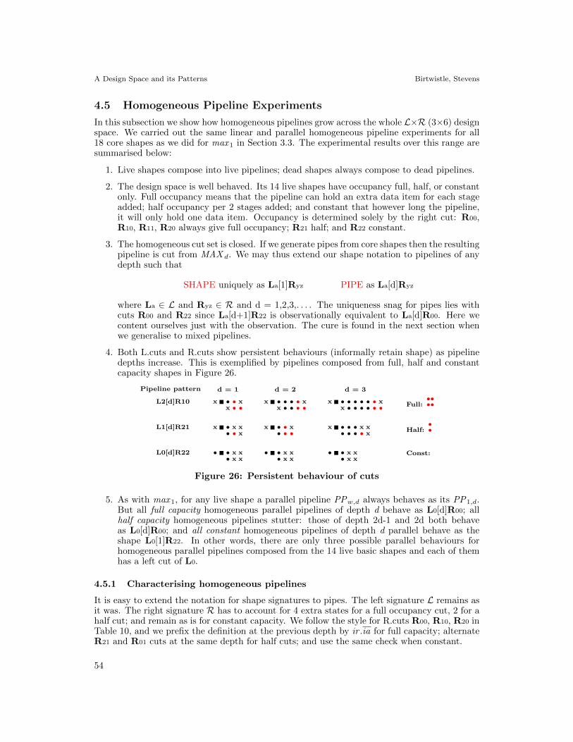
4. Both L.cuts and R.cuts show persistent behaviours (informally retain shape) as pipelinedepths increase. This is exemplified by pipelines composed from full, half and constantcapacity shapes in Figure 26.
Pipeline pattern d = 1 d = 2 d = 3
L2[d]R10
L1[d]R21
L0[d]R22
Full:••••
Half:••
Const:
x • • xx • •
x • • • • xx • • • •
x • • • • • • xx • • • • • •
x • x x• • x
x • • x• • •
x • • • x x• • • • x
• • x x• x x
• • x x• x x
• • x x• x x
Figure 26: Persistent behaviour of cuts
5. As with max 1, for any live shape a parallel pipeline PPw,d always behaves as its PP1,d.But all full capacity homogeneous parallel pipelines of depth d behave as L0[d]R00; allhalf capacity homogeneous pipelines stutter: those of depth 2d-1 and 2d both behaveas L0[d]R00; and all constant homogeneous pipelines of depth d parallel behave as theshape L0[1]R22. In other words, there are only three possible parallel behaviours forhomogeneous parallel pipelines composed from the 14 live basic shapes and each of themhas a left cut of L0.
4.5.1 Characterising homogeneous pipelines
It is easy to extend the notation for shape signatures to pipes. The left signature L remains asit was. The right signature R has to account for 4 extra states for a full occupancy cut, 2 for ahalf cut; and remain as is for constant capacity. We follow the style for R.cuts R00, R10, R20 inTable 10, and we prefix the definition at the previous depth by ir .ia for full capacity; alternateR21 and R01 cuts at the same depth for half cuts; and use the same check when constant.
54
A Design Space and its Patterns Birtwistle, Stevens
LPkLa = La
LP1R10 = R10 LP1R21 = R21 LP1R22 = R22LP2R10 = ir .ia.LP1R10 LP2R21 = R10 LP2R22 = R22LP3R10 = ir .ia.LP2R10 LP3R21 = ir .ia.LP1R21 LP3R22 = R22LP4R10 = ir .ia.LP3R10 LP4R21 = ir .ia.LP2R10 LP4R22 = R22
............... ............... ...............
Table 12: Sample linear pipeline characterisations
5 Mixed Pipeline Structures and Patterns
In this section we relate experiments carried out with linear mixed pipelines. The increase ingenerality yielded one surprise: some R.cut combinations, for example R11.R20, gave rise to aright cut of R31 (valid from depth 2). With R31 included however, the R.cuts become closed.This slight addition has important ramifications. By dispensing with cut R22, the uniquenessof pipeline representation snag noted in the previous section disappears. Further the lattice ofR.cuts may be cast as two related chains each of which has a simple mapping from the chainof L.cuts; a structure that we exploit in this section.
Notation. In this section, we use Sa.Sb as a compact notation for the linear pipeline formedby Sa and Sb. In the same way, if Sa has cuts La and Ra and Sb has cuts Lb and Rb, then wedenote the cuts of Sa.Sb by La.Lb and Ra.Rb.
5.1 Initial mixed experimentsFor linear pipeline S2 constructed from shapes Sa and Sb (Figure 27), signal or from Sahandshakes with ir of Sb and signal ia from Sb handshakes with oa of Sa. The livenessconditions thus assure the liveness of the pipeline provided that Sa and Sb are both live, bethey of full, half or constant capacity.
Sa Sb
ir
ia
or
oa
or
oa
ir
ia
Figure 27: Mixed pipeline S2 = Sa.Sb
Revised R.cuts. Initially we experimented with all 18 combinational possibilities for L.cutsand R.cuts in pipelines of depth 2. They confirmed the liveness proposition and the indepen-dence of L.cuts and R.cuts, but yielded one unexpected result: that the R.cuts were not closed.The R.cut combinations R11.R20, R21.R20, R11.R21 all combine to form a depth 2 R.cut ofR31. If we augment the set of right cuts by R31, then R.cuts becomes closed. We have alreadynoted that R22 is redundant. If we omit it, we have an R.cut set that is closed.
L : chain R : 2 chains
L0 L1 L2
R00
R11
R10
R21
R20
R31
Figure 28: Lattice structures revised
55
A Design Space and its Patterns Birtwistle, Stevens
Since the L.cuts form a chain, it is fruitful to think of the R.cuts as a lattice structure formedby two related chains R0 and R1 shown horizontally on the right of Figure 28. It is then easyto map amongst them and take advantage of the structural relationships between the outputand input cuts.
Revised pipeline notation. If we extend our definition of maximal pipelines to include thethe 4 state max 0 (= L0[1]R22)
max 0 = ir .or .oa.ia.max 0
MAX 0 = max 0
MAX d+1 = MAX d ++••••
Table 13: MAX pipelines revised
then we can express any live pipeline constructed from core shapes uniquely by cutaways fromsome MAX d. Clearly, there is just one live pipeline at depth 0, max 0 itself, which cannottolerate any cuts. There are 13 live pipelines at depth 1 (where no R31 cut will be live).Pipelines at depths 2 or more accept all 18 cut possibilities.
5.2 Experimental Results for Mixed Linear Pipelines
Our experiments paired up all shape possibilities L×R, including the non-live which served toconfirm our liveness properties. By enumeration over all cases S2 = Sa.Sb:
1. Liveness: S2 is live if and only if Sa and Sb are live.
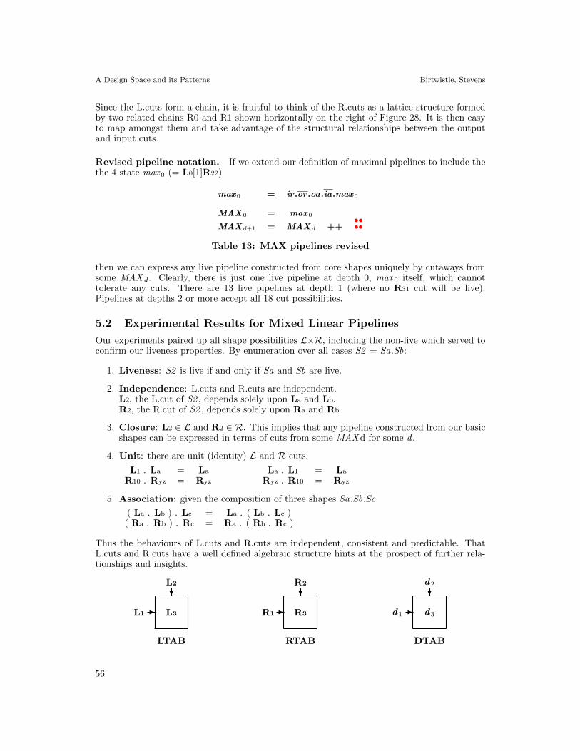
2. Independence: L.cuts and R.cuts are independent.L2, the L.cut of S2 , depends solely upon La and Lb.R2, the R.cut of S2 , depends solely upon Ra and Rb
3. Closure: L2 ∈ L and R2 ∈ R. This implies that any pipeline constructed from our basicshapes can be expressed in terms of cuts from some MAX d for some d .
4. Unit: there are unit (identity) L and R cuts.
L1 . La = La La . L1 = La
R10 . Ryz = Ryz Ryz . R10 = Ryz
5. Association: given the composition of three shapes Sa.Sb.Sc
( La . Lb ) . Lc = La . ( Lb . Lc )( Ra . Rb ) . Rc = Ra . ( Rb . Rc )
Thus the behaviours of L.cuts and R.cuts are independent, consistent and predictable. ThatL.cuts and R.cuts have a well defined algebraic structure hints at the prospect of further rela-tionships and insights.
L3 R3 d3-
?
L1
L2
LTAB
-
?
R1
R2
RTAB
-
?
d1
d2
DTAB
56
A Design Space and its Patterns Birtwistle, Stevens
5.2.1 Tabulation of LTAB, RTAB and DTAB
Because L.cuts and R.cuts work independently, we can condense their experimental propertiesin simple lookup tables. The pipeline depth of the resulting shape depends upon the constituentdepths and also upon its two R.cuts.
LTAB. Cut L1 is the unit (or identity) cut.
Table 14: LTAB
La.Lb L0 L1 L2
L0 L0 L0 L0L1 L0 L1 L2L2 L2 L2 L2
RTAB. Cut R10 is the unit cut. Notice that the row entries for R21 are related to those ofR10 and span the spectrum of R.cuts but shifted by 3.
DTAB. The data for DTAB is presented graphically. Since it partly depends upon theconstituent R.cuts, R1.R2, the results are entered in patterns of the form R1.R2 → R3.
Table 16: DTAB
Ra.Rb R00 R10 R20 R11 R21 R31
R00•••• .••••→
••••••••
•••• .••••→
••••••••
•••• .••••→
••••••••
•••• .••••→
••••••••
•••• .••••→
••••••••
•••• .••••••••→
••••••••••••
R10•••• .••••→
••••••••
•••• .••••→
••••••••
•••• .••••→
••••••••
•••• .••••→
••••••••
•••• .••••→
••••••••
•••• .••••••••→
••••••••••••
R11•••• .••••→
••••••••
•••• .••••→
••••••••
•••• .••••→
••••••••
•••• .••••→
••••••••
•••• .••••→
••••••••
•••• .••••••••→
••••••••••••
R20•••• .••••→
••••••••
•••• .••••→
••••••••
•••• .••••→
••••••••
•••• .••••→
••••
•••• .••••→
••••
•••• .••••••••→
••••
R21•••• .••••→
••••••••
•••• .••••→
••••••••
•••• .••••→
••••••••
•••• .••••→
••••
•••• .••••→
••••
•••• .••••••••→
••••
R31•••••••• .
••••→
•••••••••••••••••••• .
••••→
••••••••••••
•••••••• .
••••→
••••••••••••
•••••••• .
••••→
•••••••••••••••• .
••••→
•••••••••••••••• .
••••••••→
••••••••••••
57
A Design Space and its Patterns Birtwistle, Stevens
The NW, NE, SW quadrants contain those combinations that give rise to full occupancy. Inthese quadrants, if R1 is of depth d1 and R2 is of depth d2 then R1.R2 gives rise to a pipe oflength d1+d2. The SE quadrant contains those combinations that give rise to pipes of lengthd1+d2-1. So DTAB reveals that the calculation of pipeline depth is simple.
5.3 Calculation of Pipeline Behaviours
Space precludes any account of mixed parallel pipeline behaviours, but they too are calculable.
5.3.1 Application I: mixed linear pipe of depth 4
Once we have these tables it is straightforward to calculate the shape of any 2 stage pipeline.Because the cuts are closed, we can calculate the behaviours and properties of pipelines of anydepth. Longer pipelines may be calculated by iteration as in the following application:
and R4 = (R20.R00).R31.R11 → (R00.R31).R11 → R20.R11 → R00
and d4 = (1.0).2.1 → (1.2).1 → 3.1 → 3Thus PIPE2 = L0[1]R00 since R20.R00 lies in the SW quadrant
PIPE3 = L0[3]R20 since R00.R31 lies in the NE quadrantPIPE4 = L0[3]R00 since R20.R11 lies in the SE quadrant
Note that associativity allows us to compose these 4 shapes any way we choose as long as theirordering is respected. These predictions have all been confirmed by experiment.
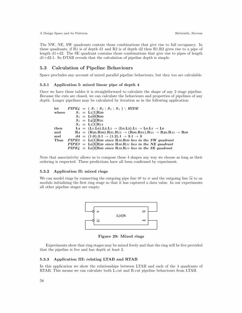
5.3.2 Application II: mixed rings
We can model rings by connecting the outgoing pipe line or to ir and the outgoing line ia to oamodulo initialising the first ring stage so that it has captured a data value. In our experimentsall other pipeline stages are empty.
L[d]R
dd iria
or
oa
Figure 29: Mixed rings
Experiments show that ring stages may be mixed freely and that the ring will be live providedthat the pipeline is live and has depth at least 2.
5.3.3 Application III: relating LTAB and RTAB
In this application we show the relationships between LTAB and each of the 4 quadrants ofRTAB. This means we can calculate both L.cut and R.cut pipeline behaviours from LTAB.
58
A Design Space and its Patterns Birtwistle, Stevens
The two cut families are related by a number of maps. As we will be operating on cuts, rowsof cuts, and (sub-)tables of cuts, we introduce two extra operators. If f is a function operatingon a cut, then ROW.f applies f to each cut in a row of cuts and TAB.f applies f each cutelement in a table of cuts. The design space is so small that we define the basic cut functionsby enumeration of cases.
L0 L1 L2
R00 R10 R20 R11 R21 R31
?
6LtoR0 R0toL
?
6LtoR1 R1toL
-
�
II
II
Figure 30: Maps between L.cut and R.cut chains
Maps between R.chain0 and R.chain1: II Rxy = R(x+1)(y+1) mod 22
Notice that the bottom half of RTAB may be obtained from the top half by applying TAB.IIand vice versa. Going laterally is more interesting.
5.4 Extension to 4phase untimed
The approach to mixed pipelines outlined in this section has been applied equally successfullyto the 10×20 untimed subset of 4phase designs; the 19×38 untimed ++ locally timed subset;and to the complete 35×140 4phase design space.
L000
L200
L400
L220
L420
L440
L222
L422
L442 L444
R0000
R0020
R0400
R0022
R0042
R0044
R2022
R2042
R2044 R4044
R2222
R2242
R2262
R2244
R2264
R2266
R4244
R4264
R4266 R6266
Figure 32: L.wedge R0.wedge and R2.wedge
Just as with 2phase, the R.cuts previously published [8, 34] were closed for homogeneouspipelines but not for mixed. Following through the techniques presented here resulted in a
60
A Design Space and its Patterns Birtwistle, Stevens
reduction of in the size of R.cuts from 25 to 20 which revealed for the first time a splittingof R.cuts into two subsets each of which is isomorphic to L.cuts as shown in Figure 32. It isdoubtful we would have made these connections without venturing into mixed pipelines andinsights gleaned from this work in the 2phase domain.
In 4phase, the L.cuts have 3 indices, Labc and R.cuts 4, Rwxyz. Each R.cut in wedge R0 hasx=0, and each R.cut in wedge R2 has x=2. Similar to the II operation for 2phase, cut Rw0yz
in wedge R0 is vertically aligned with cut R(w+2)2(y+2)(z+2) in wedge R2.It is simple to draw up the 4phase equivalents of the 2phase mapping functions of Sec-
tion 5.3.3. The structure of the 2phase transformations given in Figure 31 still holds subjectto a (simply) modified versions of the FLIP operation and II operations.
6 From Shape to Silicon
An implementation study was performed similar to that in [34]. Systematic concurrency re-duction produced by applying cuts to the most concurrent shape results in the complete designspace. This allows all possible specifications to be investigated in order to obtain the bestcircuit for any specific design goal, be it high performance, low power, small area, latency, etc.
When realizing designs, shapes are partitioned into design styles. Shapes can be catego-rized into two protocol classes, untimed and timed. Untimed shapes come in two classes: delayinsensitive (DI) and speed independent (SI). Likewise timed shapes have two classes: locallytimed (LT) and externally timed (ET). Locally timed shapes can be designed to work in nearlyall homogeneous or mixed pipelines based on the local delays present inside the circuit imple-mentation of any given shape. However, externally timed shapes are only correct when specificrelative delay requirements are enforced on the response time of other controllers. For example,the consumer (downstream controller) connected to an ET shape may be required to respondmuch faster than the producer (the upstream controller).
This paper extends previous work to include all locally timed shapes. LT shapes for the2phase family are formed by the L1 and R10 cuts. Externally timed cuts include all Ry1 cuts.Thus to investigate all DI, SI, and LT shapes, the L and top R chains from Figure 28 areemployed; the lower R chain is discarded. The 3×3 cuts result in 9 shapes categorized as oneDI, two SI, five LT and one deadlocked shape.
An automated flow was developed to generate and optimize asynchronous pipeline con-trollers from the shape state machines. The designs were synthesized and technology mappedto Artisan’s static library for IBM’s 65nm 10sf process node using Petrify [15]. The circuits
Frequency in GHz
L0 L1 L2 La[1]Ryz
4.22 4.40 4.00 R00
4.50 5.05 4.27 R10
4.20 3.78 – R20
Energy per Token in pJ
L0 L1 L2 La[1]Ryz
8.73 11.20 7.15 R00
8.90 7.95 7.75 R10
7.48 5.18 – R20
Area in µm2
L0 L1 L2 La[1]Ryz
217 243 204 R00
221 220 206 R10
207 211 – R20
Figure 33: Performance, power, and area of the circuits
61
A Design Space and its Patterns Birtwistle, Stevens
are verified for conformance to the shape, and automatic relative timing (RT) constraints arecreated [43]. The RT constraints are applied using a custom flow to synthesize and optimize thecircuits for power and performance using commercial clocked CAD tools such as Design Com-piler and SOC Encounter [40]. The results report parasitic extracted values for the physicallyplaced and routed designs.
The results for performance, power and area are shown in Figure 33. The better designsare highlighted in green, the worse designs in red. The timed L.cut and R.cut are highlightedin yellow. All rows and columns employing timed cuts result in timed shapes (5 of the 8).
The NW corner of the tables contains shapes with the most concurrency and the SE cornerthe most sequential. In general, the more concurrent shapes should admit a higher perfor-mance; the most sequential lower power and smaller area. This general trend applies with somenotable exceptions. For example, the larger and more complicated circuits required for higherconcurrency may hamper performance. But most significantly, the locally timed cuts producethe fastest circuits. The four highest frequency designs all employ timed cuts. The best timedshape produces a circuit that is 20% faster than the circuit from the best untimed shape. Onlya handful of timed circuits have been investigated and published in the literature. This studythereby opens up the possibility of uncovering new design sets with substantial performanceimprovements over current state of the art.
7 Overview and summary
We have investigated an abstract model of latch controllers and presented new experimentalresults on its outer and inner structure in terms of L and R lattices of cuts from the maximalshape. L×R reveals the whole design space and has been used to guide experiments rangingfrom investigating linear and parallel pipeline patterns through to investigating the behaviour offamilies of circuits. The patterns have suggested algorithmic rules for predicting the behavioursof homogeneous and mixed pipelines. Such predictions make it possible to replace complicatedirregular parallel datapaths by smooth linear pipeline behaviours—a very useful mental modelwhen designing systems.
Novel design space patterns herein described include: complete lattices for L and R cuts;complete design space as L×R; notation for each shape and each pipeline as La[k]Ryz; theconsistent and independent growth patterns L and R cuts; and not least in the treatmentof mixed pipelines. Demonstrations of their practical use were given for predicting pipelinebehaviours and generating novel circuits.
1. Survey of published designs (4phase). This kept our work grounded. Our common alge-braic (FSM) notation for their shapes (design abstractions) enables them to be orderedand compared. In shape format, all published designs had at least input signal orderingconstraints or output signal ordering constraints; and usually both. Taking the intersec-tion of constraints over all surveyed shapes revealed max 1, a maximal shape (most con-current possible signal orderings), from which all published shapes could be constructedby cutting away states on the Left or on the Right.
2. Taking our cue from the way input and output cuts characterised published designs, wefully generalised the cut possibilities from max 1. The product L×R reveals the completedesign space for max 1 and its sub-designs. The cut classes form elegant lattices and enabletight mathematical definitions of design style domains over max 1: e.g. delay insensitive,speed independent, burst mode, relative timing. The definitions are defined simply interms of sublattices of L and R. A software suite has been developed which will takeshape specifications and generate characterized circuits. Since we have the design space,and know how to categorize design styles, we can (and have) examined the 3×6 2phasedesign space and the 10×25 DI subset of 4phase. Work is in progress studying suchcharacteristics as: area, power consumption, speed, ...
62
A Design Space and its Patterns Birtwistle, Stevens
3. We have conducted experiments on the behaviours of homogeneous linear pipelines ofdepths 1..12 and over homogeneous parallel pipelines of depths 1..12 and widths 1..8 overthe Untimed sub-design space. These experiments revealed much persistent structuredbehaviour: examples (i) if a shape is live, then so will be its pipelines; (ii) L.cuts andR.cuts work independently of each other; (iii) all parallel compositions are observationallyequivalent to some DI single pipeline; (iv) shapes exhibit full, half, or unit occupancy;(v) occupancy is determined solely by a shape’s R.cut. For homogeneous pipelines, theL and R sets are closed, so that we can adapt the specification of a shape to define ahomogeneous pipeline of any depth
4. We have also experimented with mixed pipelines: by which we permit a linear pipeline tohave different shapes throughout its length; and with mixed parallel pipelines where wemay run distinct homogeneous (or mixed) linear pipelines in parallel. For tractable designsubsets, the results are again structured. In particular liveness, cut independence, the DIbehaviour of parallel pipes still hold. But for mixed pipelines, the R sets are not closed.However it is a simple matter to include extra R.cuts (valid only from pipeline depth 2) toensure closure. Experiments have been completed over 2phase and 4phase shapes. Theseshow that shapes associate under pipelining and that the behaviour of linear pipelines ofany depth can not only be specified in terms of the L and extended R.cuts but can alsobe calculated from their constituents. By extension, we can also calculate the behaviourof mixed parallel pipelines from their constituents.
5. The understanding and formalisation of this increase generality resulted in some dramatic(and practical) simplifications. We can now relate the L and R cut lattices and once wehave calculated the LTAB, the mixed L.cut behaviour table, we can construct RTAB themixed R.cut table by simple and standard transformations.
Acknowledgements
This work has been supported in part by a grant from Sun Microsystems.Thanks are due to the asynchronous community who have made great efforts to document
and explain their circuits so they are clear to the community at large. This body of workenabled us to model real practical designs rather than experiment with a few idealised onesand kept us grounded. Importantly, the corpus was sufficiently large to guide our researchdirections.
For their individual help and guidance over the years, we thank Erik Brunvand, Bill Coates,Jordi Cortadella, Al Davis, Jo Ebergen, Steve Furber, Jim Garside, Luciano Lavagno, AndrewLines, Ying Liu, Faron Moller, Mike Stannett, Georg Struth, Chris Tofts, and AlexanderYakovlev. They are of course in no way to blame for any lack of clarity or errors we mayhave made.
References
[1] L. Aceto, K.G. Larsen, and A. Ingolfsdottir. An Introduction to Milner’s CCS. Course Notes forSemantics and Verification. Constantly under revision. The most recent version is available at theURL http://www.cs.auc.dk/∼luca/SV/Intro21ccs.pdf, BRICS, Department of Computer Science,Aalborg, Denmark, 2005.
[2] J. M. Anderson, W. S. Coates, A. L. Davis, R. W. Hon, I. N. Robinson, S. V Robison, and K. S.Stevens. The Architecture of FAIM-1. Computer, 20(1):55–65, January 1987.
[3] E. R. Berlekamp, J. H. Conway, and R. K. Guy. Winning Ways for your Mathematical Plays.pages 598–601, London, 1982. Academic Press.
[4] G. Birtwistle and Y. Liu. Modelling AMULET1 in CCS. IEE Colloquium on Design and Test ofAsynchronous Systems, pages 9/1–9/6, 1996.
[5] G. Birtwistle and Y. Liu. Specification and Property Checking of the AMULET1 Address Interface.Designing Correct Circuits 96, 1996.
63
A Design Space and its Patterns Birtwistle, Stevens
[6] Graham Birtwistle. Control states in asynchronous pipelines. In Alex Yakovlev and ReinderNouta, editors, Asynchronous Interfaces: Tools, Techniques, and Implementations, pages 45–55,July 2000.
[7] Graham Birtwistle and Matthew Morley. Case study: specifying and property checking TK, anasynchronous AMULET-like microprocessor. In A. Yakovlev and R. Nouta, editors, AsynchronousInterfaces: Tools, Techniques, and Implementations (AINT’2000), pages 13–22, TU Delft, July,2000.
[8] Graham Birtwistle and Kenneth Stevens. The Family of 4-phase Latch Controllers. In ASYNC2008, 14th International Symposium on Asynchronous Circuits and Systems, pages 71–82, New-castle upon Tyne, UK, 7-11 April, 2008.
[9] I. Blunno, J. Cortadella, A. Kondratyev, L.Lavagno, K. Lwin, and C. Sotiriou. Handshake proto-cols for de-synchronisation. In Proceedings of the International Symposium on Advanced Researchin Asynchronous Circuits, pages 149–158. IEEE/ACM, April 2004.
[10] A. E. Brouwer, G. Horvath, I. Molnar-Saska, and C. Czabo. On three-rowed Chomp. In INTEGER:Electronic Journal of Combinatorial Number Theory, volume 5, pages 1–11, 2005.
[11] E. Brunvand. Translating Concurrent Communicating Programs into Asynchronous Circuits. PhDthesis, School of Computer Science, Carnegie Mellon University, Pittsburgh, PA, 1991.
[12] E. L. Brunvand and R. F. Sproull. Translating Concurrent Programs into Delay-insensitive Cir-cuits. In IEEE International Conference on Computer-Aided Design, pages 262–265, Los Alamitos,CA, 1989. IEEE Comput. Soc. Press.
[13] Tam-Anh Chu. Synthesis of Self-Timed VLSI Circuits From Graph-Theoretic Specifications. PhDthesis, Massachusetts Institute of Technology, September 1987.
[14] J. Cortadella, M. Kishinevsky, S. M. Burns, A. Kondratyev, L. Lavagno, K. S. Stevens, A. Taubin,and A. Yakovlev. Lazy transition systems and asynchronous circuit synthesis with relative timingassumptions. IEEE Transactions on Computer-Aided Design, 21(2):109–130, Feb 2002.
[15] J. Cortadella, M. Kishinevsky, A. Kondratyev, L. Lavagno, and A. Yakovlev. Petrify: a tool formanipulating concurrent specifications and synthesis of asynchronous controllers. IEICE Trans-actions on Information and Systems, E80-D(3):315–325, March 1997.
[16] Paul Day and J. Viv Woods. Investigation into micropipeline latch design styles. IEEE Transac-tions on VLSI Systems, 3(2):264–272, June 1995.
[17] J. Ebergen. Parallel Computations and Delay-Insensitive Circuits. In G. Birtwistle, editor, IVHigher Order Workshop, Banff 1990, pages 85–104, Berlin, 1991. Workshops in Computing Series,Springer Verlag.
[18] J. C. Ebergen, J. Segers, and I. Benko. Parallel Program and Asynchronous Circuit Design. In A.Davis and G. Birtwistle, editor, Proceedings VII Banff Workshop: Asynchronous Digital CircuitDesign, pages 50–103. Springer Verlag, Workshops in Computing Series, 1995.
[19] Aristides Efthymiou and Jim D. Garside. Adaptive pipeline structures for speculation control. InNinth International Symposium on Asynchronous Circuits and Systems, pages 46–55. IEEE, May2003.
[20] S. Furber. Computing without Clocks: Micropipelining the ARM Processor. In A. Davis and G.Birtwistle, editor, Proceedings VII Banff Workshop: Asynchronous Digital Circuit Design, pages211–262. Springer Verlag, Workshops in Computing Series, 1995.
[21] S. B. Furber, J. D. Garside, P. Riocreux, S. Temple, P. Day, J. Liu, and N. C. Paver. AMULET2e:An Asynchronous Embeded Controller. Proceedings of IEEE, 87(2):243–256, February 1999.
[22] S. B. Furber and J. Liu. Dynamic logic in four-phase micropipelines. In Second InternationalSymposium on Advanced Research in Asynchronous Circuits and Systems, pages 11–16. IEEEComputer Society Press, March 1996.
[23] Stephen B. Furber. A small compendium of 4-phase macropipeline latch control circuits. TechnicalReport v0.3, 17/01/99, University of Manchester, Dept. of Computer Science, 1999.
[24] Stephen B. Furber and Paul Day. Four-phase micropipeline latch control circuits. IEEE Transac-tions on VLSI Systems, 4(2):247–253, June 1996.
[25] Rakefet Kol and Ran Ginosar. A doubly-latched asynchronous pipeline. In Proceedings of theInternational Conference on Computer Design (ICCD), pages 706–711, Oct 1996.
[26] Andrew M. Lines. Pipelined asynchronous circuits. Master’s thesis, California Institute of Tech-nology, Pasadena, CA, 1998.
[27] JianWei Liu. Arithmetic and Control Componenets for an Asynchronous System. PhD Thesis,Department of Computer Science, University of Manchester, 1997.
64
A Design Space and its Patterns Birtwistle, Stevens
[28] A. J. Martin. Compiling Communicating Processes into Delay-Insensitive VLSI Circuits. Dis-tributed Computing, 1:226–234, 1986.
[29] A. J. Martin. Programming in VLSI: From Communicating Processes to Delay-Insensitive Circuits.In C. A. R. Hoare, editor, Developments in Concurrency and Communication, New York, 1990.Addison-Wesley.
[30] A. J. Martin. Synthesis of Asynchronous VLSI Circuits. In J. Staunstrup, editor, Formal Methodsfor VLSI Design, North Holland, 1990.
[31] Alain J. Martin. The Design of a Delay-Insensitive Microprocessor: An Example of Circuit Syn-thesis by Program Transformation. In M. Leeser and G. Brown, editors, Hardware Specification,Verification, and Synthesis: Mathematical Aspects, Proceedings of the Mathematical Sciences In-stitute Workshop, Cornell University, Ithaca, N.Y., July, 1989, pages 244–259, New York, 1989.Springer-Verlag.
[32] R. Milner. Communication and Concurrency. Prentice-Hall, London, 1989.[33] Faron G. Moller and Perdita Stevens. The Edinburgh Concurrency Workbench (Version 7). Uni-
versity of Edinburgh, October 1992.[34] Santosh Nagasai, Kenneth Stevens, and Graham Birtwistle. Concurrency Reduction of Untimed
Latch Protocols – Theory and Practice. In International Symposium on Asynchronous Circuitsand Systems (ASYNC), pages 26–37, Grenoble, France, May 2010.
[35] Montek Singh and Steven M. Nowick. High-throughput asynchronous pipelines for fine-graindynamic datapaths. In 6th International Symposium on Advanced Research in AsynchronousCircuits and Systems, pages 198–209. IEEE, Apr 2000.
[36] Montek Singh and Steven M. Nowick. MOUSETRAP: Ultra-High-Speed Transition-SignalingAsynchronous Pipelines. In Proceedings of the International Conference on Computer Design(ICCD), pages 9–17, Nov 2001.
[37] Kenneth S. Stevens, Ran Ginosar, and Shai Rotem. Relative Timing. IEEE Transactions on VeryLarge Scale Integration (VLSI) Systems, 1(11):129–140, February 2003.
[38] Kenneth S. Stevens, Shane V Robison, and A.L. Davis. The Post Office – Communication Sup-port for Distributed Ensemble Architectures. In Proceedings of 6th International Conference onDistributed Computing Systems, pages 160 – 166, May 1986.
[39] Kenneth S. Stevens, Shai Rotem, Ran Ginosar, Peter Beerel, Chris J. Myers, Kenneth Y. Yun,Rakefet Kol, Charles Dike, and Marly Roncken. An Asynchronous Instruction Length Decoder.IEEE Journal of Solid State Circuits, 36(2):217–228, February 2001.
[40] Kenneth S. Stevens, Yang Xu, and Vikas Vij. Characterization of Asynchronous Templates forIntegration into Clocked CAD Flows. In 15th International Symposium on Asynchronous Circuitsand Systems, pages 151–161. IEEE, May 2009.
[41] C. Stirling. Modal and Temporal Properties of Processes. Springer Verlag, New York, Berlin,Heidelberg, 2001.
[42] Ivan E. Sutherland. Micropipelines. Communications of the ACM, 32(6):720–738, June 1989.Turing Award Paper.
[43] Yang Xu and Kenneth S. Stevens. Automatic Synthesis of Computation Interference Constraintsfor Relative Timing. In 26th International Conference on Computer Design, pages 16–22. IEEE,Oct. 2009.
[44] Eslam Yahya and Marc Renaudin. QDI Latches Characteristics and Asynchronous Linear-PipelinePerformance Analysis. In Integrated Circuit and System Design, Power and Timing Modeling,Optimization and Simulation, Lecture Notes in Computer Science, pages 583–592. Springer, 2006.
[45] A. Yakovlev, L. Lavagno, and A. Sangiovanni-Vincentelli. A unified signal transition graph modelfor asynchronous control circuit synthesis. Formal Methods in System Design, 9:139–188, 1996.
[46] Kenneth Y. Yun, Peter A. Beerel, and Julio Arceo. High-performance asynchronous pipelinecircuits. In Second International Symposium on Advanced Research in Asynchronous Circuits andSystems, pages 17–28. IEEE Computer Society Press, March 1996.