NASA-CR-199755 lf1 if Research Institute for Advanced Computer Science NASA Ames Research Center A Deterministic Particle Method for One-Dimensional Reaction-Diffusion Equations Michael Mascagni r (NASA-CR-199755) A DETERMINISTIC PARTICLE METHOD FOR ONE-DIMENSIONAL REACTION-DIFFUSION EQUATIONS (Research Inst. for Advanced Computer Science) 17 p N96-15853 Unclas G3/64 0083947 RIACS Technical Report 95.23 November, 1995 https://ntrs.nasa.gov/search.jsp?R=19960008687 2018-05-22T05:11:21+00:00Z
Transcript
NASA-CR-199755
lf1if
Research Institute for Advanced Computer ScienceNASA Ames Research Center
A Deterministic Particle Method forOne-Dimensional Reaction-Diffusion
Equations
Michael Mascagni
r(NASA-CR-199755) A DETERMINISTICPARTICLE METHOD FOR ONE-DIMENSIONALREACTION-DIFFUSION EQUATIONS(Research Inst. for AdvancedComputer Science) 17 p
The Research Institute of Advanced Computer Science is operated by Universities Space ResearchAssociation, The American City Building, Suite 212, Columbia, MD 21044, (410) 730-2656
Work reported herein was supported by NASA via Contract NAS 2-13721 between NASA and the UniversitiesSpace Research Association (USRA). Work was performed at the Research Institute for Advanced ComputerScience (RIACS), NASA Ames Research Center, Moffett Field, CA 94035-1000.
A DETERMINISTIC PARTICLE METHOD FORONE-DIMENSIONAL REACTION-DIFFUSION EQUATIONS
MICHAEL MASCAGNI
RIACS, NASA Ames Research Centerand
Center for Computing Sciences, I.D.A.
ABSTRACT. We derive a deterministic particle method for the solution of nonlinear reaction-diffusion equations in one spatial dimension. This deterministic method is an analog of aMonte Carlo method for the solution of these problems that has been previously investigatedby the author. The deterministic method leads to the consideration of a system of ordinarydifferential equations for the positions of suitably defined particles. We then consider thetime explicit and implicit methods for this system of ordinary differential equations and westudy a Picard and Newton iteration for the solution of the implicit system. Next we solvenumerically this system and study the discretization error both analytically and numerically.Numerical computation shows that this deterministic method is automatically adaptive tolarge gradients in the solution.
1. Introduction.We are interested in numerical methods for the solution of nonlinear reaction-diffusion
equations in one species and in one spatial dimension. These equations can be studied asinitial-value problems and have the form:
(1) ut = vuxx + /(u), i > 0, ,it(a;,0) = tt0(a;), v > 0.
Partial differential equations (PDEs) of this form are often found in multi-species systemsthat model phenomena from chemical combustion to excitability in neurons [10, 7, 11].
A qualitative feature of solutions to (1) is that they often have sharp gradients andtraveling fronts. Because of this, standard finite-difference methods often require very finegrids to resolve the sharp gradients. With a traveling front solution the gradient is steepestin a small region that moves with the front. An optimal finite-difference method wouldincorporate moving refined grids into a numerical solution algorithm.
An alternative is to consider a Monte Carlo method for the solution of (1). Such anapproach yields a particle-based method that is automatically adapting to sharp gradients,[18, 19, 20]. The major drawback with a Monte Carlo approach is that convergence is
1991 Mathematics Subject Classification. 65CM99, 92C20.Key words and phrases, reaction-diffusion equations, particle methods, numerical analysis, automatic
adaptivity.
Typeset by
2 A DETERMINISTIC PARTICLE METHOD
stochastic and can be shown to behave as O(Ar~1 '2), where N is the number of particles,[21]. An advantage of the Monte Carlo approach is that its particle-based formulation canserve as a starting point for the construction of a deterministic analog. This paper exploressuch a deterministic particle method for monotonic solutions to equation (1).
The plan of the paper is as follows. In §2 we briefly review a one-dimensional MonteCarlo method, called the gradient random walk (GRW) method, for (1) and recall it's
. major qualitative and quantitative properties. In §3 we derive the deterministic analogfor monotonic solutions to equation (1). This leads to an interesting system of ordinarydifferential equations (ODEs) that has nonlinearities corresponding to the linear diffusionterm in (1) and is linear where (1) is nonlinear! In §4 we discuss some common boundaryconditions for reaction-diffusion equations and techniques for incorporating them into thisnumerical method. In §5 we consider the forward and backward Euler methods for thesolution of the resulting ODEs. The backward Euler method leads to consideration ofa nonlinear tridiagonal system. A Picard iteration is shown to solve this system; and aNewton's method solution is also analyzed. In §6 we present some numerical results forthe Nagumo equation, a scalar reaction-diffusion equation with monotonic solutions thatmodels nerve conduction. These numerical results motivate an analysis of the discretizationerror. This error can be further broken down into an error in the wave speed, that canbe analyzed analytically, and a static discretization error, that can be studied numerically.Finally, in §7 we conclude by summarizing our results and discussing the extension of thismethod to multi-species reaction-diffusion systems and to higher dimensions.
2. Monte Carlo Algorithms.We first review the gradient random walk (GRW) method [1, 5, 19] for equation (1). We
assume that u(- , t ) is monotonic, i.e., u(x,t) < u(y,i) when x < y, and that u(— oo,i) =0,u(+oo,<) = 1. The strategy is to represent v = ux by diffusing particles. We choose touse a particle representation for the gradient since integration of the gradient to recoverthe solution is a variance reduction technique. Differentiating (1) with respect to x,
(2) vt = vvxx + /'(u)u, u(x,0) = «{,(x),
and discretizing v as a sum of ^-functions with strength rrij , we have
N
(3) v(x,t)
where Xj(t),j = 1, . . . , Ar represent the location of the N particles. We use capital X toindicate that the positions are random variables. The density of the particles determinesthe value of v, and heuristically one thinks of mj as the "mass" of the jth particle.
We recover u from v by u(x,t) = Jj^ v(x' ,i): dx' :
N
(4) u(x,t)
M. MASCAGNI 3
Thus u is represented as a step function with jumps of size irij at Xj. If all the particleshave the same mass, 77^, the value of u at x is m times the number of particles that lie tothe left of x. The boundary condition at — oo is automatically satisfied, and the conditionat +00 is satisfied on average, with fluctuations [19]. This corresponds to conservation ofmass.
As described in [5], there is much less noise in the computed value of u than of v becauseall the particles contribute to the value at any point, x. Moreover, if the particles haveequal mass, their density is large precisely where u has large gradients.
Once the initial data is discretized, the GRW method evolves the particle positions andmasses such that u satisfies equation (1). This is done by a fractional step iteration inwhich the diffusion term is modeled by a random walk and the reaction term is modeledas exponential growth-or decay of the particle masses. For each time step the sequence is:
A. Gaussian Random Walk Step:
where the <Jj are independent JV(0, 2i/Atf) random variablesB. Evaluate uj = u(Xj(t + Arf)) , j = 1, . . . ,N using (4)C. Kill or Replicate Particles: with probability |/'(wj)|Atf
i. Kill particle if /' < 0ii. Create a new particle at Xj if /' > 0
Note that the only way the particles interact with each other, and hence the only way thatthe nonlinearity of the equations is manifest in the algorithm, is that the local value of udepends on the positions of all the particles. Not surprisingly, this is the step that is mostdifficult computationally. Naively, computing equation (4) for all the Xj's requires O(N2)work, but if the particles are sorted, it requires only O(N) work plus O(N log N} for thesorting.
The variant of this method due to Chorin and Ghoniem [1, 12, 5] is essentially thesame, except that instead of killing and replicating particles, the masses are increased ordecreased according to the ordinary differential equation
= '<•>>•In the mean and to O(At) the two procedures are equivalent.
Both methods have been used to solve traveling-wave problems in one-dimension. Themechanism of wave propagation is transfer of mass from behind the front to ahead of it.With randomized particle death and replication, particles are killed off behind the wavefront, where /'(•) is mostly negative, and replicated ahead of the front, where /'(•) is mostlypositive. With deterministic particle growth and decay, there is a graded transmission ofmass from neighbor to neighbor.
3. The Deterministic Algorithm.Among both the different Monte Carlo algorithms we discussed in the previous section,
the Chorin- Ghoniem variant already contains deterministic elements. However, it requires
4 A DETERMINISTIC PARTICLE METHOD
using time dependent masses for the particles. What we seek is a totally deterministicalgorithm where the masses of the particles remain constant and equal throughout thecomputation. This kind of algorithm has been applied to convection-diffusion equationsbefore [3, 6, 13, 15, 16, 17], and we wish to extend these methods to reaction-diffusionproblems.
To begin our derivation, let us assume that we have a monotonic solution to (1), u(x,t)with 0 < u(x,t) < 1 for alH > 0 and u(—oo,i) = 0, u(-foo,i) = 1. Then we may define thefunctions Xi(t) implicitly by saying they mark the locations of where the solution attainscertain values as:
(5) u(Xi(t),t) = ^, i = l , 2 , . . . ,N-2 ,N- l , t > 0 .
Obviously we have that xo(t) = —oo and £/v(t) = +00. We now seek equations of motionfor the Zi(-)'s given, that they satisfy (1). Let us take the total derivative with respect totime of (5):
(6) d fcteW'*)! = o = «,(*,-(*), *)*(*) + u,(*,-(0, *).
A rearrangement of (6) gives:
Equation (7) gives an expression for the velocity of the zth marker point, ii(tf), in termsof certain derivatives of u and values of /(u(-)). We have defined the values of u at thepoints £j(t), so let us use those values to evaluate the terms above. Let us denote u(xi(t), t)as «,-. Using formally second order finite-difference approximations we first approximate:
-1 Xi+iM-Xi- i t t ) NUx(X i(t) , t) Ui+i-tt;-! 2
Next we approximate:
u;+ i— u,- U j — U j - i
(9)
Finally it is obvious that
(10)
M. MASCAGNI
so that the resulting equation becomes:
(11) Xt = V —"o"
This equation is very odd in the sense that its linear terms correspond to the nonlinearterms of the PDE (1) and visa versa. The first term on the right-hand side of (11) is highlynonlinear and corresponds to the linear diffusion term of (1), while the nonlinear j(u] termof the PDE results in the second (linear) term of (11). This is not, however, the completesystem to consider. Usually equation (1) is part of an initial- value or initial boundary-valueproblem. Thus we must consider ways of incorporating the various boundary conditionsassociated with these problems into this curious formulation.
4. Boundary Conditions.
The system of ODEs in (11) is quite contrary with regard to linear and nonlinear terms.It is also a contrarian with regard to boundary conditions since the most natural problemto discretize is the pure initial-value problem with a monotonic solution. The pure initial-value problem on the entire line presents difficulties for finite- difference and finite-elementmethods. In these cases either explicit methods are used and only that subset of the linecontaining the dynamic parts of the solution is included in the computation, or an artificialboundary is used. With this deterministic particle method no such ad hoc approach isrequired.
Another way that this discretization is contrary to finite-difference and finite-elementmethods is that here we perform a uniform discretization of the dependent variable, u. Infinite-difference and finite-element methods it is space, an independent variable, that isdiscretized to give a system of ODEs. While this traditional approach makes certain typesof error analysis more convenient, discretization of the solution permits computationalelement, the particles, to concentrate automatically in areas where the solution is changingmost rapidly.
For the monotonic pure initial- value problem we have that xo(t) — — oo and xiv(t) = +00at all times, and so x0(t) = i;v(i) = 0. For i = 2, . . . , N — 2 we can just apply equation (11).The difficulty arises for i = I and i = N — I since equation (11) involves the points XQ andXN in the terms involving /. These difficulties can be avoided if we go back to the derivationfor these two equations and rederive them, being mindful to avoid the singularities. Wemay think of the ODEs in (11) as a result of combining the ODEs derived from the particlemethod discretization of the two equations (a) ut = vuxx and (b) ut = f(u) under the
assumption of a monotonic solution. Discretization of (a) yields x, \ = v\ - - --- - - ,-1 \ / - X{— X i — i x;_|-i— Xi '
which is valid at i = 1 and i = N — 1, as the terms involving the infinite quantities are zero.To rederive (b) let us use the relevant part of equation (7). This means consideration of
* « • * = " 0 - A t ? ; = i w eat n — N — 1 we have ux(xpj-i(t) , t) K j^- - ^ - y. These along with the contributions
6 A DETERMINISTIC PARTICLE METHOD
from (a) give the following system for the pure initial-value problem:
XQ = 0,
, i = 2, . . . ,JV-2,X{ Xi — i ^i+l
Similarly, Dirichlet boundary conditions are. easy to impose with this particle method.Consider first a time independent Dirichlet boundary condition:
(13) u(Q,t) = U0, u(l,*) = Z7i, U 0 < U i . '
Here the solution is to rescale the problem so that UQ = 0 and Ui = 1 and use the conditionsXQ = 0 and a;TV = !• The situation is a bit more complicated when the Dirichlet boundaryconditions are time-dependent:
Since we have discretized u in our particle method, time-dependent boundary conditionsrequire the creation and destruction of particles along the boundary. For example, if Uo(t)is increasing and in some time interval gains N~l in value, the left-most particle's positionmust be set to zero. This has the effect of increasing the value of the solution at zero byTV"1. Conversely, if Uo(t) is decreasing and diminishes by TV"1 in value, a new particle isintroduced at zero. At x = 1 we use a similar strategy, except that we remove a particlewhen Uo(t) decreases and insert a particle when Uo(t) increases.
In many cases Neumann boundary conditions are appropriate. The time-independentversion of these conditions
Since we are restricting our method to monotonic solutions, we must have ux(0,t) > 0and « r( l ,<) > 0. Let us first consider the leftmost boundary condition. Suppose that theleft-most particle is at the location x\ > 0. An estimate of the derivative is thus
(16) ti,(0,0 w ̂ ^ = ̂ - = U0 -» Xl = l
Xi 1\ Xi
Similarly, at the right-hand side assume that rryv-i is the right-most particle in the unitinterval, then the right-hand Neumann condition becomes xjv-i = 1 — jjjj--
It should be clear that time-dependent Neumann boundary conditions are really nomore trouble. Indeed, if we have the conditions:
(17) 'u*(0,t) = U0(t), ««(!,*) = CM<), tfo(*)>0, t/,(*)>0.They are enforced via: x\(t) = NJ ,t) and XA'-I(^) = 1 — Nl} ,ty One important pointis that we are constrained to keep these particles in the unit interval so that 1 > xi(t) =
Nv i t
time.and 0 < .r/v-i(i) = 1 — j v t / o ? which means that A^ > ^ and N > -y for all
M. MASCAGNI 7
5. Time Discretizations.Let us now consider some simple time discretizations of (11). We will consider only
the forward- and backward- Euler methods here, which are first order methods. However,the analysis of the backward-Euler method will indicate the magnitude of the stiffnessexpected in these ODEs when solved by other implicit methods, [4].
Let us consider the pure initial-values problem that results in the system of ODEs in(12). Let us first give this equation the vector notation: x(t) = F(x(i)), where x(i) =(xQ(t) ,xi( t ) , . . . ,XN-i ( t ) ,XN(t ) ) T and jF(x(i)) is the right-hand side of (12). We nowintroduce a time discretization with time step Atf and Xj = x(_? Ai) so that the forwardEuler method is merely:
(18)
With our particular F(-), this equation is known to converge to the exact solution asAt ^ 0 as 0(A<), [2]. In fact, it can be shown that if m-m i [ ( x i + l_^ ) ( x i_X i_ l ) } < ± thisdifference equation is numerically stable. This fact is very much analogous to the stabilityof the forward- Euler method for a finite- difference solution to these same equations, [8, 14].
Because of the serious time-step restriction, we should consider the fully implicit backward-Euler method:
xn+1 - xn+1 = xn.
This equation forms a nonlinear tridiagonal system. To see this let us consider the ?'thequation of equation (19):
1 1 1 TV / ? \± -1 _|_ A4_ fj-n+1 _ rn+M f I — I — rn
,-n+l _ n-+l Tn+l _ n+l M~ 9 ^ '+1 l'~1 ' \ N I ~~ i '"i ^i-l ^i+l xz J \-L /
(20) <+1 -
The second term corresponds to the linear diffusion term in (1), and it can be simplifiedby reduction to a common denominator. Let us define A'""1"1 = ,,+i — n+i^/ n+i — ̂ RT so
(xi ~x i- i )(xi+i ~xi >that equation (20) becomes:
jn+l n+l , Jn+l n+l , n+l n+l _ n'i Xi-i ~r "t Xi "T Ui Xi+l — Xi '
(21)
Solving (21) requires dealing with a very odd nonlinear system. Even if the nonlinearterms from diffusion are held constant (the A'"+1's), the linear system in (21) is not
A DETERMINISTIC PARTICLE METHOD
guaranteed to be diagonally dominant.1 However, a simple Picard iteration that willconverge is possible if we rearrange (21) to allow us to work with a diagonally dominantsystem. Let us put the terms involving /(•) on the right-hand side as follows:
(22)
U+ 1 = -A2A+ 1 .
This nonlinear system is 'diagonally dominant, and so the Picard iteration defined as followswill converge, [9]:
A. Initialization: x°/d = xn
B. Iterate until converged:i. Solve the following for xneu):
roldLi —
Dold =
(23) U°ld = -Lrold new i r\old newLJ £.-_i ~r u .t^ ~T- ly •*/t+]
— 1 ^T?'rf — ?'rfTVJ^Hi *,-!
ii. Set X°W = x"ew
C. Form the solution to (22) as xn+1 = xnew.
Notice that the linear system in (23) is of the same form as one encounters in a finite-difference solution to (12). In fact, instead of the term L°ld = —AiA"°'rf we would have
in the finite-difference case. These terms are very much analogous. Note that thedenominator of — AiA"f'rf = 7—^73 — 0i7T^liJ - OTT IS ̂ e product of two neighboring variable
Vxi xi-i)(.xi + i xi )
spatial grid spacings, just like in the finite- difference case.Now let us consider solving (21) with a Newton iteration. Recall that the Newton
method iteration for the solution to the nonlinear system G(x) = 0 is defined implicitlyby the equation J(x0jrf)(xneiu — x0/d) = — G(x0/<i). Here the Jacobian matrix, J, haselements defined by [J]^- = |jf . For equation (21) we have
(24) C,.(x) = *,-
1 Diagonal dominance guarantees both nonsingularity and the numerical stability of Gaussian elimina-tion without pivoting, the Thomas algorithm. Without diagonal dominance we must pivot, which slowsdown the computation.
M. MASCAGN1
where the final, converged, solution gives xn+i. Thus J has the form:
-i/A* i NA1'A1 i NAl r I _ t_ \-i,-)2 "*" 2 •' V A'/ ' = 7
— I
i/At(z,- + i— i-,-)J (
'A/ A'Af /(ii-i,-_i)2 " 2 ^
o,
*A/
( « \ iV N) ' ^ ' L
otherwise.
(25)
The matrix J is tridiagonal with a very curious form: it is the sum of a strictly di-agonally dominant symmetric matrix and a real antisymmetric matrix. The result is atridiagonal matrix that, in general, cannot be thought of as diagonally dominant. How-ever, for most cases of interest this system will be diagonally dominant but not symmetric.Since we are adding and subtracting the same number from the off diagonals, the ma-trix will remain diagonally dominant if [Jjn+i < 0. This requirement is equivalent to
vAt ^ NAt f f j-^ Replace the term involving / with its maximum on the unit/ \ 2 s^ ry
interval, fm ax = rnaxre[0)i] /(a;), and divide by AtN2 to give r^, . "l-x.)u > 2lv
Now the term t N r x . 1 _ x . s i2 is an approximation to the square of the first derivative. Sincethe solution we seek is monotonic, this is always bounded away from zero by a constant,H~1 > 0, thus we rewrite this equation as N > 3™°* . Since the right-hand side is con-stant, choosing N larger makes the inequality true; thus by choosing N sufficiently large,the system can be made diagonally dominant.
6. Numerical Results.In this section we consider the numerical solution of Nagumo's equation, [11], as part
of a pure initial value problem:
(26) ut = uxx + u(l — u)(u — a), t > 0, u(x,0) = UQ(X), 1 > a > 0.
In this pure initial-value problem setting, Naugmo's equation has a stable traveling wavesolution given by u(x,t) — *_ ^, where the wave speed is 9 = ^/2,(a — |). When
a = | we have 0 = 0, and the solution is a stable standing wave. These properties areeasy to check numerically and make Nagumo's equation a good candidate to explore theproperties of a new numerical method for this class of problems.
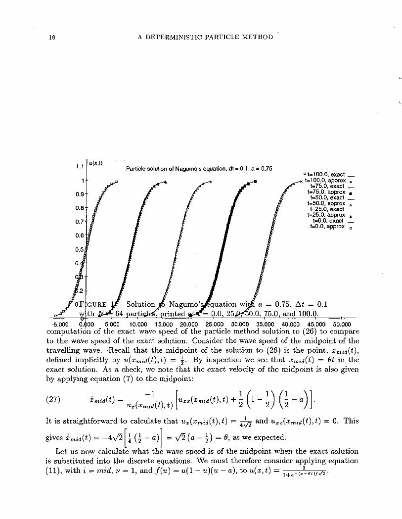
We begin by computing numerically the solution to Nagumo's equation with our particlemethod using UQ(X) = IxiJ?- This implies that u(x,i) — -ix-et^iJs- m figure 1>i "r c * IT~C \-below, we plot the computed solution at uniformly spaced times for the case where a = 0.75,with N = 64 and A< = 0.1. Notice that the particles move with the solution tracking thesteep gradient. In addition, by the end of the computations every single particle has movedpast the position of the rightmost particle in the initial configuration. This shows how thismethod is naturally adapting to the solution and is equitable in its distribution of particles.
A qualitative observation that can be noticed by scrutinizing figure 1 is that the particlesseem to be moving slightly away from the exact solution. This observation seems to indicatethat actual wave speed of the particles may be slightly greater than 0, the wave speed ofthe exact solution. Fortunately, one calculation that we can carry out explicitly is the
10 A DETERMINISTIC PARTICLE METHOD
u(x,t)Particle solution of Nagumo's equation, dt = 0.1, a = 0.75
Solution Jo Nagumo'sjquationpartigle^f rinted f= 0.0, 25J
°t=100.0, exactt=100.0, approx x
t=75.0, exactt=75.0, approx ,t=50.0, exact
t=50.0, approx 4t=25.0, exact
t=25.0, approx At=0.0, exact
t=0.0, approx D
a = 0.75, Atf = 0.1.Q, 75.0, and 100.0.
-5.000 O.ljlOO 5.000 10.000 15.000 20.000 25.000 30.000 35.000 40.000 45.000 50.000computation of the exact wave speed of the particle method solution to (26) to compareto the wave speed of the exact solution. Consider the wave speed of the midpoint of thetravelling wave. -Recall that the midpoint of the solution to (26) is the point, xmid(t),defined implicitly by u(xm id(t)>t) — |. By inspection we see that xmid(t) = 9t in theexact solution. As a check, we note that the exact velocity of the midpoint is also givenby applying equation (7) to the midpoint:
(27) ). 0 + l ~2
It is straightforward to calculate that ux(xmid(t},i) = T^= and uxx(xmid(t),t) = 0. This
gives xmid(t) = -4\/2 | (| — a) = \/2 (a — |) = 6, as we expected.
Let us now calculate what the wave speed is of the midpoint when the exact solutionis substituted into the discrete equations. We must therefore consider applying equation(11), with t = mid, v = 1, and /(u) = u(l - u}(u - a), to w(x,<) =
M. MASCAGNI 11
First we show that the diffusion term in (11) zero for Nagumo's equation. Assume weha.ve N points in our discretization, where N is even. Hence mid = y. We also have that
t0 §ive X»"d+lt = 0t-
1). Similarly, xmid-i(t) = 9t — V2li~i( mt^_1 — 1), so that the differences in the diffusionterm are given by:
l f NIn
mid + 1 I \ mid
N
(28)
Zmid-l = - >/2( N \ ( N
„! —— — 1 I — In I ——\tmd J \rrnd — 1
->/21nmid—1
Now we compute:
K N — l\ / N — 1\ 1mid+1 \ / mid—1 \
N 1 I N ' 1 •
The numerator of the term inside the logarithm can be rewritten as:(30)
N A / JV _ \ _ N2 N N-I J \rnid — I J (mid + l)(mid — 1) mid — I mid + I
And thus (xmid+\ — xmid) = (xmid — ̂ mtd-i), thus making the diffusion term in (11)vanish. For convenience, in the sequel we will refer to the common value of this differenceas h.
Thus we are left to consider the equation
(31) xmid(t) = -
The term ^-2,h is the reciprocal of the centered difference approximation to the first deriv-ative. Indeed it is the case that(32)
h* ux x x(xm i d , t)_ux(xm i d , t )+ !£uxxx(xmid,t) + 0(h*) u x (xm i d , t ) [ 6 u
12 A DETERMINISTIC PARTICLE METHOD
For the exact solution one can show that u
stated that ux(xm id(t) , t ) — -7^75= so thatgives:
id i
= ^-T=. Recall that above we
— |. Substituting this into (31)
-/(I)(33)
Equation (33) implies that the computed solution should have (1) a velocity that isslightly greater than the actual solution, and (2) this difference in velocity goes to zerowith h2. Intuition suggests that h oc -^, so one can think of the error in the velocity asgoing to zero with the square of the number of particles. We notice both these phenomenain our computations.
TABLE 1. The error in the wave speed (9) in the particle methodsolution to Nagumo's equation. Errors for various values of a and N arepresented.
To confirm this calculation we have computed the velocity of xmid(t] for various valuesof a, and hence various values of #, and with various (power-of-two) numbers of points.We have tabulated our results in table 1. A logarithmic regression actually gives the errorin the wave speed as O(N~ 2) instead of the expected O(N~2).
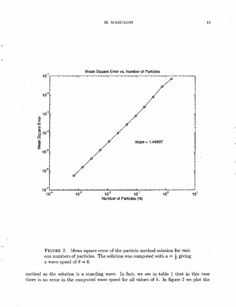
We have now computed the systematic error in the wave speed of our numerical method.The overall error in our numerical method is the sum of this error, which should be O(i),and the error in the solution is due only to the spatial discretization. Nagumo's equationallows us to study this second type of error directly by examining the numerical solutionwhen a=| and 6 = 0. In this case we expect that the numerical solution will deviate fromthe exact solution only, due to what is "discretization" error for this peculiar numerical
M. MASCAGNI 13
10"Mean Square Error vs. Number of Particles
10
10"
-2
LU<D
COccaa>
-510
10"
10-7
slope = 1.49897
10" 10"Number of Particles (N)
10U 10'
FIGURE 2. Mean square error of the particle method solution for vari-ous numbers of particles. The solution was computed with a = | givinga wave speed of 9 = 0.
method as the solution is a standing wave. In fact, we see in table 1 that in this casethere is no error in the computed wave speed for all values of h. In figure 2 we plot the
14 A DETERMINISTIC PARTICLE METHOD
asymptotic mean square error in the particle method solution versus the number of pointsused. Notice that the slope of the curve in figure 2, a log-log plot, is w —1.5, meaning thatthe the error behaves as O(N~?}. Thus the overall error of our method is O(N~?) .
7. Conclusions.We have derived an adaptive particle method for the solution of one-dimensional reaction-
diffusion equations with monotonic solutions. This method is the deterministic analog ofa Monte Carlo method for these same problems. Like the Monte Carlo method, this de-terministic method uses a discretization of the solution to obtain a method that naturallytracks the solution by resolving the gradient. Thus this method is particularly suited toequations which have very steep gradients in the solution. We have also analyzed thedifference equations associated with this discretization and have proposed a Picard andNewton iteration for the solution of the nonlinear system of equations arising from thefully implicit backward Euler time discretization. We have also decomposed the error inthe method into the error in computing the wave speed and the spatial discretization er-ror. This former error can be asymptotically computed, while the later has been studied
»
numerically. The overall error in the method appears to be O(N~ 2). This is much betterthan the O(N~?) error in the Monte Carlo method.
Many questions remain. The most important question being why is the accuracyO(N~?) when we have chosen a spatial discretization based on second order accuracy?Perhaps the difference equations themselves can be refined to give a more accurate formu-lation. Or, the method of imposing the boundary conditions was only first order. Thismay have contaminated the overall accuracy of the solution. Is there a better formulationfor the boundary conditions? It is also important to consider how to extend this method.Three ways that one would like to extend this method is to include (i) nonmonotonic butpositive solutions, (ii) multi-species systems, and (iii) several spatial dimensions.
REFERENCES1. A. J. Chorin, Numerical methods for use in combustion modeling, Computing Methods in Applied
Sciences and Engineering (R. Glowinski and J. L. Lions, eds.), North Holland, Amsterdam, 1980,pp. 229-235.
2. E. A. Coddington and N. I. Levinson, Theory of Ordinary Differential Equations, McGraw-Hill, NewYork, 1955.
3. P. Degond and F.-J. Mustieles, A deterministic approximation of diffusion equations using particles,SIAM. J. Sci. Stat. Comput. 11 (1990), 293-310.
4. C. W. Gear, Numerical Initial Value Problems in Ordinary Differential Equations, Prentice-Hall,Engelwood Cliffs, New Jersey, 1971.
5. A. F. Ghoniem and F. Sherman, Grid-free simulation of diffusion using random walk methods, J.Comput. Phys. 61 (1985), 1-37.
6. F. Hermeline, A deterministic particle method for transport diffusion equations: Application to theFokker-Planck equation, J. Comput. Phys. 82 (1989), 122-146.
7. A. L. Hodgkin and A. F. Huxley, A quantitative description of membrane current and its applicationto conduction in the giant axon of Loligo, J. Physiol. 117 (1952), 500-544.
8. E. Isaacson and H. B. Keller, Analysis of Numerical Methods, John Wiley and Sons, New York, 1966.9. M. Mascagni, The backward Euler method for the numerical solution of the Hodgkin-Huxley equations
of nerve conduction, SIAM J. Num. Anal. 27 (1990), 941-962.10. H. P. McKean, Jr., Application of Brownian motion to the equation of Kolmogorov-Petrovskii-
Piskunov, Communications on Pure and Applied Mathematics XXVIII (1975), 323-331.11. J. Nagumo and S. Arimoto and S. Yoshizawa, An active pulse transmission line simulating nerve
axon, Proc. IRE 50 (1962), 2061-2070.
M. MASCAGNI 15
12. A. K. Oppenheim and A. Ghoniem, Application of the random element method to one-dimensionalflame propagation problems, AIAA-83-0600, AIAA 21st Aerospace Sciences Meeting, Reno, NV, 1983.
13. P. A. Ravi art, An analysis of particle methods, Numerical methods in fluid dynamics (F. Brezzi, ed.),Lecture Notes in Mathematics, 1127, Springer-Verlag, New York, 1985.
14. R. D. Richtmeyer and K. W. Morton, Difference Methods for Initial Value Problems, Second Edition,Interscience Publishers, division of John Wiley and Sons, New York, London, Sydney, 1967.
15. G. Russo, A particle method for collisional kinetic equations. I Basic theory and one-dimensionalresults, J. Comput. Phys. 87 (1990), 270-300.
16. G. Russo, Deterministic diffusion of particles, Communications on Pure and Applied MathematicsXLIII (1990), 697-733.
17. G. Russo, A Lagrangian method for collisional kinetic equations, Proceedings of the 1988 AMS SIAMSummer Seminar, Colorado State University, Fort Collins, Colorado, July 18-29, 1988 (E. L. All-gower and K. Georg, eds.), Lectures in Applied Mathematics, 26, American Mathematical Society,Providence, Rhode Island, 1990, pp. 519-539.
18. A. S. Sherman and M. Mascagni, A gradient random walk method for two-dimensional reaction-diffusion equations, SIAM Journal on Scientific Computing 15 (1994), 1280-1293.
19. A. S. Sherman and C. S. Peskin, A Monte-Carlo method for scalar reaction diffusion equations, SIAMJ. Sci. Stat. Comput. 7 (1986), 1360-1372.
20. A. S. Sherman and C. S. Peskin, Solving the Hodgkin-Huxley equations by a random walk method,SIAM J. Sci. Stat. Comput. 9 (1988), 170-190.
21. D. Talay, Simulation and numerical analysis of stochastic differential systems: A review inbookEffective Stochastic Analysis (1990), Inria (Report #1313), Valbonne, France, 1-51.
RIACS; NASA AMES RESEARCH CENTER; M/S T20G-5; MOFFETT FIELD, CAL-IFORNIA 94035-1000; CENTER FOR COMPUTING SCIENCES, I.D.A.; 17100 SCIENCEDRIVE; BOWIE, MARYLAND 20715-4300


![Blended Particle Filters for Large Dimensional Chaotic ...qidi/publications/Blended... · Particle filtering of low-dimensional dynamical systems is an es-tablished discipline [9].](https://static.documents.pub/doc/80x56/5fa3ddbe2c17b6242816e21a/blended-particle-filters-for-large-dimensional-chaotic-qidipublicationsblended.jpg)
