A Diabetes minimal model for Oral GlucoseTolerance Tests

J. Andres Christena∗, Marcos Capistrana,Adriana Monroyb, Silvestre Alavezc, Silvia Quintana Vargasd

Hugo A Flores-Arguedasa and Nicolas KuschinskiaaCIMAT, Guanajuato, Mexico

bHospital General, Mexico City, MexicocUAM, Lerma, Mexico

dDIF/Hospital Alta Especialidad, Guanajuato, Mexico

January 2016

Abstract

We present a minimal model for analyzing Oral Glucose ToleranceTest (OGTT) data base on system of 5 ODEs. The model has 4unknown parameters which are inferred using a Bayesian approach.Preliminarily results are shown with three real patient data.

1 Introduction

For diagnosis of diabetes, metabolic syndrome and other conditions an OralGlucose Tolerance Test (OGTT) is performed. After a night’s sleep, fastingpatients have their blood glucose measured and are asked to drink a 75 gsugar concentrate. Blood glucose is then measured at the hour, two hoursand sometimes at three hours, depending on local practices.

A diagnosis tool is needed since there are many scenarios in which bloodglucose ranges from low to high to intermediate levels in different patternsand MD’s resort only to simple guidelines for diagnosis.

∗(corresponding author) Email: jac@cimat.mx .

1

arX

iv:1

601.

0475

3v1

[st

at.A

P] 1

8 Ja

n 20

16

Table 1: Minimal model for analysis of OGTT state variables, parame-ter definition and units. Time is measured in hours (hr) and therefore allderivatives have corresponding units per hr.

Units Interpretation Value

G mgdL Blood glucose. State variable

I mgdL (see text) Blood Insulin. State variable

L mgdL (see text) Blood Glucagon. State variable

D mgdL Glucose in digestive system. State variable

V mgdL Glucose in the drinkable solution, State variable

to be transferred to the digestive system.

θ0 hr−1 Insulin tissue sensitivity. Unknown par.

θ1 hr−1 Glucagon liver sensitivity. Unknown par.

θ2 hr Glucose digestive system mean life. Unknown par.

a, b hr Insulin and Glucagon clearance mean life. 31 min.

c hr Time that the subject took to drink most of the 5 min max.glucose solution (transfer time to D).

We develop a minimal model for blood glucose-insulin interaction basedon a two compartment model. A a simple transfer compartment of glucoseinto the diagestive system and a more complex compartment for blood glu-cose and interactions with Insulin and other glucose substitution mechanisms.

Once OGTT data is available, we perform a formal statistical analysisusing Bayesian inference for the unknown parameters of each patient andpredict their glucose level at 3h after the test.

2

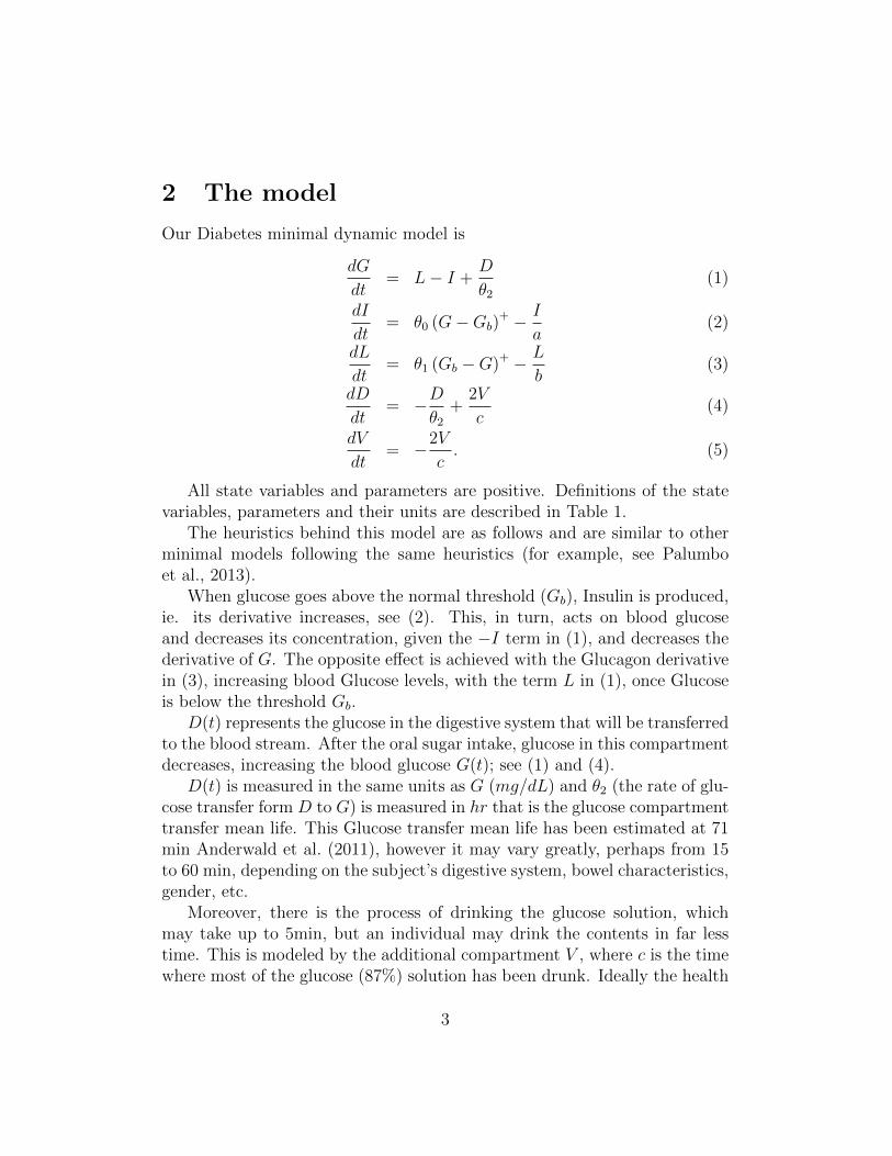
2 The model

Our Diabetes minimal dynamic model is

dG

dt= L− I +

D

θ2(1)

dI

dt= θ0 (G−Gb)

+ − I

a(2)

dL

dt= θ1 (Gb −G)+ − L

b(3)

dD

dt= −D

θ2+

2V

c(4)

dV

dt= −2V

c. (5)

All state variables and parameters are positive. Definitions of the statevariables, parameters and their units are described in Table 1.

The heuristics behind this model are as follows and are similar to otherminimal models following the same heuristics (for example, see Palumboet al., 2013).

When glucose goes above the normal threshold (Gb), Insulin is produced,ie. its derivative increases, see (2). This, in turn, acts on blood glucoseand decreases its concentration, given the −I term in (1), and decreases thederivative of G. The opposite effect is achieved with the Glucagon derivativein (3), increasing blood Glucose levels, with the term L in (1), once Glucoseis below the threshold Gb.

D(t) represents the glucose in the digestive system that will be transferredto the blood stream. After the oral sugar intake, glucose in this compartmentdecreases, increasing the blood glucose G(t); see (1) and (4).

D(t) is measured in the same units as G (mg/dL) and θ2 (the rate of glu-cose transfer form D to G) is measured in hr that is the glucose compartmenttransfer mean life. This Glucose transfer mean life has been estimated at 71min Anderwald et al. (2011), however it may vary greatly, perhaps from 15to 60 min, depending on the subject’s digestive system, bowel characteristics,gender, etc.

Moreover, there is the process of drinking the glucose solution, whichmay take up to 5min, but an individual may drink the contents in far lesstime. This is modeled by the additional compartment V , where c is the timewhere most of the glucose (87%) solution has been drunk. Ideally the health

3

practictioner would record the total time the patient took to drink the glucosesolution. Unfortunately this information is not available and therefore we fixc = 5/60hr.

The Insulin and Glucagon clearance rates are not estimated. It is knownthat the total Insulin clearance time is approximately 71 min (Duckworthet al., 1998); we therefore set the Insulin half life to 36min, that is a = 0.6hr.There is less knowledge regarding clearance rates for Glucagon. We set itequal to the clearance rate of Insulin, that is b = 0.6hr.

3 Uncertainty Quantification Using Bayesian

Inference

Once the OGTT data is observed we perform the Inverse Analysis by infer-ring the patient’s corresponding model parameters using Bayesian statistics(Fox et al., 2013). We have observations d0, d1, . . . , dn−1 for the measuredGlucose during the OGTT test at times t0, t1, . . . , tn−1. Plasma glucose ismeasured with relative precision, however high frequency fluctuations exist(given the pancreatic beta cells’ Insulin delivery mechanisms, idf.org (2015))and, along with model error itself, we expect Glucose readings di to fluctuatearound a mean value, modeled here as G(ti). We impute an independentGaussian error for these readings, namely

di = G(ti) + ei where ei ∼ N(0, σ); i = 0, 1, . . . , n− 1.

To account for observation errors and, at least informally, model uncertaintywe use a σ = 5. From this a likelihood is constructed.

As mentioned in the previous section the only parameters being inferredare θ0, θ1 and θ2. Moreover, the initial value G(0) is also a parameter tobe inferred. These are all positive and as a first choice we select Gammapriors for the parameters θ0 and θ1. Since we would like to learn about thesetwo parameters for each patient, we use vague Gamma distributions withshape=2 and rate=1

4.

The rest of the initial values are set to I(0) = 0 and L(0) = 0 since thepatient is expected to be in homeostasis (equilibrium) and D(0) = 0 fasting.V (0) = V0 is the initial Glucose intake, at the onset of the test.

On the other hand, we do have information regarding θ2, the glucosetransfer mean life. This transfer cannot be arbitrarily fast or slow, given the

4

transit through the digestive tract and the fact that the drinkable Glucosesolution is basically directly taken into the blood requiring no digestive pro-cess. The Glucose half life in the digestive tract has been estimated to bebetween 40 and 90 min Anderwald et al. (2011).

We use a gamma distribution with mean at 1/2hr (shape= 10 and rate=20) and truncated at the extreme (but bounded) values 0.16 < θ2 < 2.That is, most sugar will be transferred (2θ2) to the blood stream withinin a minimum of 20 min and a maximum of 4hr. In fact, since (4) and(5) may be regarded as a separate system of ODEs (forcing the system of(1), (2) and (3) with the term D

θ2), which in turn may be regarded as a

linear nonhomegeneous ODE, it may be solved analytically for D to obtain

D(t) = V0c

2θ2−1

(e−

2tc − e−

tθ2

). Since D cannot be negative, at t = 0 it may

only increase, therefore D′(0) > 0. From this it is straightforward to see thatwe most have θ2 > c/2. The support of θ2 most start above zero.

The basis of Bayesian analysis is the posterior distribution for all param-eters. This results in

f(θ|D) ∝ exp

{1

2σ2

n−1∑i=0

(di −Gθ(ti))2

}2∏j=0

θaj−1i exp(−bjθj)ISj(θj),

where aj and bj are the Gamma hyper parameters for the prior of θj, S1 =S2 = (0,∞) and S3 = [1/6, 2]. To obtain Monte Carlo samples from this(unnormalized) posterior distribution, an MCMC is performed using the t-walk (Christen and Fox, 2010). This is a self-adjusting MCMC algorithmand the resulting sampler is efficient in most cases for this low dimensional(3) problem. In the next Section we present some examples of how our modeland inference works on some real OGTT data.

4 Examples and Results

Figures 1, 3 and 5 show how real OGTT data is adjusted by our model. Thered dots are the measured data points, and the grey lines are elements of aposterior sample of glucose curves.

Figure 1 is a healthy patient, figure 2 shows the marginal priors of θ0,θ1 and θ2 corresponding to this patient, overlaid with a histogram of themarginal posteriors. Figure 3 is a patient with strange oscillating blood glu-cose measurements (previous diagnosis technique would classify this patient

5

Figure 1: A nice decaying OGTT, belonging to a healthy patient

as “normal”), and figure 4 shows the corresponding priors and posteriors.Figure 5 is a considered and Impaired Glucose Tolerant patient (IGT, cur-rently considered an pre diabetic condition) and figure 6 shows the corre-sponding posteriors for this patient.

As can be seen in all three cases, the model has strong descriptive powerfor the times contained in the measurement interval. It also has reasonablepredictive power for times beyond the interval before the patient returns toa fasting glucose level. After that the predictive power tapers off because theuncertainty in θ1 is typically very high – usually matching the uncertainty inthe prior for this parameter, except in the case of the oscillating data.

5 Conclusions

In general, the main indicator of the status of a patient is θ0. For normalpatients, θ0 is around 2. Significantly lower values indicate that a patientmay have diabetes and higher values may indicate that a patient has someother complication. The data is almost always very informative for θ0. Moreover, the bayesian inference allows for prediction, and we are able to predict

6

(a) (b) (c)

Figure 2: Priors and posteriors for the normal patient (used to generate figure1). In green are the priors of θ0(a), θ1(b), and θ2(c). In blue are histogramsof the corresponding posterior samples.

Figure 3: Data with an oscillating fit. Older diagnostic techniques wouldhave called this patient “normal”.

7

(a) (b) (c)

Figure 4: Priors and posteriors for the patient with oscillating data (used togenerate figure 3). In green are the priors of θ0(a), θ1(b), and θ2(c). In blueare histograms of the corresponding posterior samples.

Figure 5: A diabetic patient with normal fasting OGTT and an Insulinresistance profile.

8

(a) (b) (c)

Figure 6: Priors and posteriors for the insulin resistant patient (used togenerate figure 5). In green are the priors of θ0(a), θ1(b), and θ2(c). In blueare histograms of the corresponding posterior samples.

Glucose levels beyond the length of the test (shown in figure 1, 3 and 5 upto 3 h). In particular, for figure 5 the prediction is that the patient will stillhave a high glucose level (above 120 mg

dL) and yet current diagnosis standards

classify her/him as IGT (a pre diabetic condition).θ1, on the other hand, depends on measurements found below fasting

glucose levels. For healthy patients and also for diabetics, it is uncommonfor such data to become available for the duration of the test.

θ2 is an important element of inference, and often data provide informa-tion for it however, as yet, there is no clear relationship between the value ofθ2 and a patient diagnosis.

We intend to provide a tool for proper diagnosis using OGTT. For thisvery important public health issue, there is a need for a more sophisticatedtool than the direct recording of values read during the test.

Covariates (weight, age, etc.) will be used to help in the analysis, creatinga hierarchical model embedded into the ODE model, in more populationbased studies, using ideally a large sample of patients with a range of healthconditions to tune the model parameter value ranges to establish a morecomprehensive diagnosis tool than what is currently available.

A more extensive validation of the model, and model parameters, isneeded in order to have an effective diagnosis tool. This will necessarilyinvolve the OGTT tests, and their further analysis using our model, in awide range of healthy individuals and individuals with a various prediabeticand diabetic conditions to establish a more comprehensive diagnosis toolthan what is currently available.

9

We are in the course of such research and our results will be publishedelsewhere.

References

Anderwald, C., A. Gastaldelli, A. Tura, M. Krebs, M. Promintzer-Schifferl,A. Kautzky-Willer, M. Stadler, R. A. DeFronzo, G. Pacini, and M. G.Bischof (2011, Feb). Mechanism and effects of glucose absorption during anoral glucose tolerance test among females and males. J. Clin. Endocrinol.Metab. 96 (2), 515–524.

Christen, J. and C. Fox (2010). A general purpose sampling algorithm forcontinuous distributions (the t-walk). Bayesian Analysis 5 (2), 263–282.

Duckworth, W. C., R. G. Bennett, and F. G. Hamel (1998). Insulin degrada-tion: Progress and potential. Endocrine Reviews 19 (5), 608–624. PMID:9793760.

Fox, C., H. Haario, and J. Christen (2013). Inverse problems. In P. Damien,P. Dellaportas, N. Polson, and D. Stephens (Eds.), Bayesian Theory andApplications, Chapter 31, pp. 619–643. Oxford University Press.

idf.org (2015). France. http://www.idf.org/membership/eur/france. Ac-cessed: 2015-05-04.

Palumbo, P., S. Ditlevsen, A. Bertuzzi, and A. D. Gaetano (2013). Math-ematical modeling of the glucoseinsulin system: A review. MathematicalBiosciences 244 (2), 69 – 81.

10