Page 1
Opleiding Master of Science in de geologie
Academiejaar 2014–2015
Scriptie voorgelegd tot het behalen van de graad
Van Master of Science in de geologie
Promotor: Prof. Dr. E. Verleyen
Co-promotor: Dr. M. Van Daele
Leescommissie: Prof. Dr. S. Bertrand, Prof. Dr. W. Vyverman
A diatom-based reconstruction of late Quaternary
climate changes in a sediment core of Lago
Castor, North Patagonian Chilean Andes.
Delphine Van Goethem
Page 3
I
ABSTRACT IN DUTCH
De laatste decennia is een duidelijke antropogene invloed op het klimaat op te merken met
verschillende veranderingen als gevolg. Hierdoor is veel kennis over deze
klimaatsveranderingen vervaardigd. Dankzij het doorgronden van het huidige klimaatsysteem
trachten mensen accurate voorspellingen te maken over de klimaatsfluctuaties in de toekomst.
Om de hedendaagse klimaatsverschijnselen volledig te begrijpen, dient men eerst het vroegere
klimaat grondig te bestuderen samen met zijn wijzingen tot aan het huidig klimaat. Met
grondig bestuderen worden niet enkel de klimaatsmechanismen bedoeld, maar ook de
invloeden op de omgeving met al zijn biologische, fysische en chemische facetten en de
bijhorende reacties onderling. De paleoklimaten kunnen niet rechtsreeks onderzocht worden,
hiervoor wordt beroep gedaan op klimaatsarchieven die onrechtstreeks informatie bevatten
over een paleoklimaat. Voorbeelden van zulke gebruikte klimaatsarchieven zijn ijskernen,
koraalriffen, boomringen of bijvoorbeeld mariene en meersedimenten.
De studie op het proglaciale Lago Castor (45,6°S en 71,8°W, noordelijk Chileens
Patagonië) bevat meersedimenten waarop geofysische, sedimentologische en diatomeeën
analyses werden toegepast om zo een gefundeerde klimaatsreconstructie te maken doorheen
het Late Quartair. Wanneer een klimaatsverandering optreedt, zal de samenstelling in
diatomeeën, evenals de absolute diatomeeën abundanties, de sedimentologische kenmerken en
geofysische eigenschappen fluctueren. De reden voor deze veranderingen in de
diatomeeënsamenstelling is dat iedere diatomeeënsoort een specifiek habitat verkiest. Door
het samenvoegen van de resultaten van de diatomeeënanalyse, het sedimentologische en
geofysische onderzoek werd getracht een zo accuraat mogelijk paleoklimaat en de bijhorende
omgeving te reconstrueren.
Lago Castor, gelegen in het noordelijke deel van Chileens Patagonië, aan de westelijke
kant van het Andesgebergte bestaat uit twee deelbekkens, waarbij de boring van de kern
plaatsvond in het oostelijke deelbekken van het meer. De provincie Coyhaique, waarin Lago
Castor gelegen is, behoort tot de Long Liquine Ofqui fault-zone een ‘stike-slip’ breuksysteem,
dat een onderdeel is van de Southern Volcanic zone. Deze specifieke ligging van Lago Castor
heeft als gevolg dat het gebied meermaals getroffen is geweest door vulkanische activiteit,
wat zichtbaar aan de hand van de verschillende tefra lagen in de meerafzettingen. Het huidige
klimaat in de omgeving is een warm matig nat klimaat doorheen een volledig jaarverloop
waardoor de vochtigheidsgraad hoog is. De aanwezige Westerlies winden, de El Nino
Page 4
II
Southern Oscillation (ENSO), de Antarctic Oscillation (AO) en de Pacific Decal Oscillation
(PDO) beïnvloeden het huidige klimaat, maar waren ook aanwezige factoren tijdens het
Holoceen.
De diatomeeën (Phylum Bacillariophyceae) zijn eencellige eukaryotische
fotosynthetische algen, die voornamelijk voorkomen in waterige omgevingen. Deze algen
vormen de basis van de marine voedselketen en leveren 30% van de zuurstofproductie in de
wereld, hierdoor is het uitermate belangrijk om deze organismen te bestuderen nu en
doorheen de tijd. Sinds 200 miljoen jaar komen deze algen voor, waardoor de huidige
diversiteit en abundantie zeer hoog zijn. De hoeveelheid, de groei en het type van de
diatomeeën in een omgeving zijn afhankelijk van de temperatuur, nutriënten status, licht
absorptie, turbulentie, sedimenten pollutie, ijsbedekking en de biotische interacties tussen de
omgeving en de aanwezige organismen. Al deze factoren worden beïnvloed door het
aanwezige klimaat, waardoor ze wederzijds iets zeggen over het vroegere klimaat, wanneer
deze onderzocht worden. De diatomeeën worden opgesplitst in twee afzonderlijke groepen, de
Centrales en de Pennales, waarbij de soorten classificatie gebaseerd is op de vorm,
aanwezigheid of afwezigheid van bepaalde structuren, grootte, ligging en de combinatie van
verschillende structuren in de diatomeeëncel. De gebruikte karakteristieken bij de
determinatie van de aanwezige diatomeeën in de boorkern van Lago Castor zijn: de raphe, de
portulae, de copulae en de al dan niet aanwezige interne valven.
De boorlocatie van Lago Castor was gebaseerd op de reflectie seismische data, die
verkregen waren in een eerder onderzoek. Na het verkrijgen van de boorkern werd deze
geopend, beschreven, gefotografeerd en geanalyseerd door middel van een MSCL systeem.
Een eerste zonering werd gemaakt via een macroscopische beschrijving met aandacht op de
sedimentkleur, textuur, structuur en de korrelgrootte, waarna de magnetische susceptibiliteit
(MS) en de spectrofotometrische parameters (L, a*, b*) werden geanalyseerd. Uit deze
resultaten was het mogelijk om een indicatie van het chlorofyl en de carotenoïden te
verkrijgen door middel van een relatieve absorptie band diepte (RABD) van de 610 en het
minimum van de 660 en de 670 golflengten.
Uit het ouderdomsmodel bleek dat de sedimentatiesnelheid tussen 670 en 17420 cal
jaar BP een lineaire trend kent, waarna deze verhoogd tot 19655 cal jaar BP gevolgd wordt
door een hiaat tot op 41380 cal jaar BP. De voornaamste lithologie van Lago Castor bestaat
uit grove donker gekleurde silt sedimenten met alternaties van zand en hoe dieper gelegen,
Page 5
III
hoe minder zand aanwezig is. Daarnaast zijn er meerdere donkere grove tefra lagen afgezet in
de kern. De MS waarden fluctueren doorheen de volledige kern, waarbij de hoogste waarden
overeenkomen met de tefra lagen en de lagere met de diatomeeënrijke lagen.
Hierna werd de diatomeeënanalyse toegepast op de meersedimenten waarbij de stalen
eerst geoxideerd en gereinigd werden volgens de Holant-procedure, waarna de preparaten
vervaardigd werden. Nu kon de determinatie van de verschillende aanwezige diatomeeën
beginnen met het daaropvolgende tellen van de individuen. Uit de tellingresultaten werden de
absolute diatomeeën abundanties berekend en een Broken-stick analyse uitgevoerd, waaruit
bleek dat de kern opgesplitst kon worden in vijf afzonderlijke zones. De diatomeeënanalyse
werd gedaan tot 850 cm diepte, maar de kern liep tot 1000 cm waardoor er een zesde zone
aanwezig is zonder een analyse van diatomeeën. In totaal werden er 39 verschillende taxa
gevonden, waarvan zes planktonische Centricate, 13 tychoplanktonische Araphide en 20
benthische diatomeeën. De dominante taxa in Lago Castor zijn Aulacoseira granulata,
Discostella stelligera en Staurosirella.
‘Zone 6’ (1000 - 850 cm; 18620 - 17420 cal jaar BP) was gekenmerkt door hoge MS
waarden voor silt rijke sedimenten met een matige hoeveelheid aan magnetische mineralen.
De lage chlorofyl waarden gecombineerd met de MS resultaten wijzen op een extreem lage
hoeveelheid diatomeeën die verklaard kon worden door een onstabiele omgeving met een
mogelijkheid van lichtabsorptie. De lichte kleur van de sedimenten en het extreem weinige
organische materiaal in deze siltsedimenten suggereerden de aanwezigheid van een koud
droog klimaat, waarin het proglaciaal meer volledig uitgedroogd was. Dit klimaat werd
bevestigd door de extreem lage percentages van de Nothofagus en Misodendrum pollen van
Markgraf et al. (2007). In 17500 cal jaar BP vond een snelle sterke opwarming plaats,
waardoor er een versterking in het smelten van de ijskappen optrad.
In ‘zone 5’ (850 – 771 cm; 17420 – 16270 cal jaar BP) was er een stijging in chlorofyl
en totale diatomeeën abundantie, wat indicaties zijn voor een verhoging in lichtabsorptie in
een stabielere levensomgeving. De taxa die frequent voorkomen in deze zone waren de
benthische Navicula, Rhopalodia, Pinnularia, Gyrosigma, Gomphonema, Diploneis, de
tychoplanktonische Staurosirella, Pseudostaurosira en de planktonische Discostella
mascarenica. Al deze taxa kwamen veelvuldig voor in oligotrofische ondiepe meren met een
hoog alkalisch karakter, verhoogde saliniteit en hoge concentraties voor stikstof en silicium.
De stijging in organisch materiaal en de aanwezigheid van donkerdere sedimenten
Page 6
IV
suggereerden een kleine toename in vegetatie in deze periode en dit was ook bevestigd door
een lage toename in pollen abundanties. De lage pollen percentages en de diatomeeën
indicaties suggereerden een droog klimaat wat ook bleekt uit de verhoogde vuur frequenties
en magnitudes, gebaseerd op de koolafzettingen in Mallin Pollux door Markgraf et al. (2007).
Het klimaat van 17420 tot 16270 cal jaar BP was koud en droog, waarbij het meer een
oligotrofisch karakter had met een hoge alkaliniteit en grote hoeveelheden van silicium. De
temperaturen in deze periode waren hoger dan die van de LGM, maar bereikten niet de
waarden van de opwarmingspuls van 17500 cal jaar BP.
‘Zone 4’ (771 – 625,25 cm; 16270 – 13460 cal years BP) bevatte lage relatieve
percentages voor de planktonische Centricate diatomeeën en hoge abundanties voor
Staurosirella, Pseudostaurosira en Staurosira, terwijl de benthische taxa en Fragilaria
soorten gekenmerkt werden door lagere waarden dan in ‘zone 5’. Deze bemerkingen indiceren
een eerder koud klimaat waarbij een stijging in het water niveau van het meer plaatsvond. De
daling in chlorofyl, toename in carotenoïden, aanwezigheid van donkerdere sedimenten, de
lage vuur frequenties en magnitudes en de stijging in organisch materiaal impliceerden een
daling in de absorptie van licht door de versterkte wind activiteit van de Westerlies met de
bijhorende toename in precipitatie in het gebied. Het klimaat van 16270 tot 13460 cal years
BP was een koud vochtig klimaat, waar het meer een hoge alkaliniteit, turbulentie en nitraat
concentraties had boven een zandige bodem.
De dominante taxa in ‘zone 3’ (625,25 – 542 cm; 13460 – 11110 cal jaar BP) waren
Aulacoseira granulata, Discostella stelligera en Staurosirella, terwijl het meest opvallende de
aanwezigheid was van Aulacoseira humulis. De dominante Staurosirella kende echter een
daling in deze zone, wat ook het geval was voor Staurosira var venter en Staurosira
contruens en de benthische taxa. Cyclostephanos patagonicus en Discostella stelligera
fluctueerden doorheen heel deze zone, wat impliceerde dat het aanwezige klimaat ook
alterneerde van 13460 tot 11110 cal jaar BP. De toename in chlorofyl, de aanwezigheid van
donkere sedimenten en de stijging in organisch materiaal suggereerden op de aanwezigheid
van warme klimaatscondities, waarbij de vegetatie uitbreidde. De variërende vuur frequenties
waren tevens indicaties voor het alterneren van het klimaat doorheen deze periode, waarbij de
vuur events stegen tussen 13460 en 12000 cal jaar BP door waarschijnlijk de aanwezigheid
van een droge omgeving. Uit al deze proxies bleek dat het klimaat van 13460 tot 12300 cal
jaar BP warm en vochtig was, gevolgd door het Huelmo-Mascardi Cold Reversal met koude
Page 7
V
droge klimaatscondities en een hoge wind activiteit. De daaropvolgende 500 jaar was het
klimaat warmer en vochtiger, waarna de temperaturen weer daalden tot aan 11110 cal jaar BP.
De belangrijkste diatomeeën in ‘zone 2’(542 – 397 cm; 11110 – 7790 cal jaar BP)
waren Aulacoseira granulata, Discostella stelligera, Aulacoseira ambigua, Cyclostephanos
patagonicus and Staurosirella. De combinatie van deze diatomeeën suggereerde een koud
klimaat, waarbij het meer een sterke verticale menging en turbulentie kende met de
aanwezigheid van een hoge saliniteit en rijk aan nitraat en silicium. De turbulentie was
hoogstwaarschijnlijk veroorzaakt door een verhoogde windactiviteit van de Westerlies en dit
werd ook geïnsinueerd door de verhoogde vuur frequenties en magnitudes tijdens het begin
van het Holoceen. De donkere kleur van de sedimenten in combinatie met het verhoogde
organische hoeveelheid en de stijging in de Nothofagus pollen suggereerden een
aanwezigheid van een vochtig klimaat. Dit alles duidde op een warm vochtig klimaat met een
verhoogde seizoenaliteit, waarbij de zomers droog en warm zijn, terwijl de winter natte koude
condities kende. Deze periode was gekend als het ‘Early Holocene Climatic Optimum
(EHCO).
Aulacoseira granulata, Aulacoseira humulis, Discostella stelligera, Staurosirella,
Staurosira var venter, Staurosira contruens en Discostella mascarenica waren de
kenmerkende diatomeeën uit ‘zone 1’ van 7610 tot 6765 cal jaar BP. Een gematigd vochtig
klimaat was aanwezig met een gemiddelde wind activiteit van de Westerlies, waarin Lago
Castor een diep alkalirijk, silicium rijk verswater meer was. De stijgende trend in chlorofyl,
diatomeeënabundanties, pollenpercentages, donker organisch materiaal en het weinige
voorkomen van vuur events suggereerden eveneens vochtige omstandigheden. Het klimaat
van 7610 tot 6765 cal jaar BP was gematigd en vochtig en werd beïnvloed door de aanwezige
Westerlies met zijn neerslag. Van 6765 - 4100 cal jaar BP waren er hoge abundanties van
Aulacoseira granulata, humulis en Discostella stelligera, terwijl de tychoplanktonic
Staurosirella lage relatieve percentages had. Deze samenstelling in diatomeeën was
kenmerkend voor een warm klimaat met grote hoeveelheden neerslag, dat aangevoerd werd
door een versterkte Westerlies windactiviteit. Een diep alkalirijk meer met verhoogde
fosforconcentraties en de aanwezigheid van verticale menging met bijhorende turbulentie, wat
bleek uit deze diatomeeënsamenstelling. Het lage chlorofyl, de hoge hoeveelheid organische
materialen en het weinig voorkomen van vuur duidden ook op de aanwezigheid van vochtige
omstandigheden. Het klimaat van het Midden Holoceen was een gematigd vochtig klimaat
met veel precipitatie aangevoerd door de Westerlies. Van 4100 tot 2000 cal jaar BP waren
Page 8
VI
Discostella stelligera, mascarenica, Aulacoseira humulis en Aulacoseira granulata de meest
dominante diatomeeën en deze beschreven een warm klimaat met drogere condities in
vergelijking met de twee omgevende zones. De lagere hoeveelheid in Nothofagus pollen,
organisch materiaal en de stijging in vuur activiteit wezen eveneens op een daling in
vochtigheid. Een gematigd warm droog klimaat was aanwezig van 4100 tot 2000 cal jaar BP,
waarin Lago Castor verhoogde nutrienten status had met voornamelijk verhoogde
concentraties silicium. Uit de stijgende chlorofyl waarden, de dalende vuur frequenties, de
verhoogde diatomeeënabundanties en het toegenomen organische materiaal in de laatste 2000
jaar, kon gesuggereerd worden dat een gematigd zeer vochtig klimaat aanwezig was door een
versterkte activiteit van het ENSO fenomeen, waardoor er een verhoogde hoeveelheid
neerslag viel en een stijging in de effectieve vochtigheidsgraad teweegbracht.
Naast de resultaten van de diatomeeënanalyse op de meersedimenten van Lago Castor
waren er echter weinig andere studies uitgevoerd op diatomeeën in Noord Chileense
Patagonië in het Andes gebied. Hierdoor is er een noodzaak aan extra onderzoek in deze regio
zodat er een gedetailleerde klimaatsreconstructie gegenereerd kan worden van Chileense
Patagonië met meer oog voor detail. Tevens kunnen er extra analysen worden toegepast op de
meersedimenten van Lago Castor, bijvoorbeeld de diatomeeënonderzoeken onder een grotere
vergroting door middel van SEM evenals de bovenste 38 cm verzamelen van de bodem in
Lago Castor zodat informatie verworven kan worden over LIA, die in deze laatste 670 jaar
voorkwam.
Page 9
VII
ACKNOWLEGDEMENTS
This paper would have never been finished without the support, the dedication and the
patience of some wonderful people, therefore I would love to say the following words to
them.
First of all, I would like to thank Professor Dr. E. Verleyen and Dr. M. Van Daele for
the opportunity to work on this interesting research as my thesis subject and their enthusiasm
in teaching and guiding me through the entire year. I am also extremely grateful for their
patience, guidelines and comments, because of this I was able to grow in the world of
scientific research. Besides Professor Verleyen and Van Daele, I would like to thank the
laboratory assistant T. Verstraete, who explained and showed me many procedures in the
laboratory. A sincere thank you to W. Van Nieuwenhuyze and E. Van De Vijver for the
introduction in programming of Tilia, R and the determination in the world of Chilean
diatoms. A thanks to P. Kempf to help me with the Geotek core logger problems and N. Praet
for the guidance in Grapher and CorelDraw. Next many thanks to E. Boes and S. Eeckhout for
the ideal breaks.
Last but not least, I would like to thank my family, especially my sister Laurence, who
always believed in me even when I did not! You were the driving force behind my patience
and my persistence through this year.
Thank you all!!!
Page 10
VIII
TABLE OF CONTENTS
ABSTRACT IN DUTCH ............................................................................................................ I
ACKNOWLEGDEMENTS .................................................................................................... VII
TABLE OF CONTENTS ...................................................................................................... VIII
LIST OF FIGURES .................................................................................................................. XI
1. INTRODUCTION .................................................................................................................. 1
1.1. Research objectives ......................................................................................................... 1
1.2. Thesis structure ............................................................................................................... 2
2. THE LAGO CASTOR AREA ............................................................................................... 4
2.1. The lake basin of Lago Castor ......................................................................................... 4
2.2. The hydrology and the lake classification ....................................................................... 4
2.3. The geological setting of the North Patagonian Chilean Andes ..................................... 5
2.4. The glacial history of the North Patagonian Chilean Andes ........................................... 8
2.5. The paleoclimate from the Last Glacial Maximum ........................................................ 9
2.6. The present day climate at Lago Castor ........................................................................ 11
2.6.1. Basics of climate today of North Patagonian Chilean Andes ................................ 11
2.6.2. EL Niño Southern Oscillation (ENSO) .................................................................. 14
2.6.3. Antarctic Oscillation (AO) ..................................................................................... 16
2.6.4. Pacific Decadal Oscillation (PDO)......................................................................... 17
3. DIATOMS ............................................................................................................................ 18
3.1. What are diatoms? ......................................................................................................... 18
3.2. The classification of diatoms ......................................................................................... 19
3.3. The general characteristics of diatoms .......................................................................... 20
3.3.1. Diatom habitats ...................................................................................................... 20
3.3.2. The diatom structure ............................................................................................... 20
3.3.3. The reproduction of diatoms .................................................................................. 22
4. MATERIALS AND METHODS ......................................................................................... 23
Page 11
IX
4.1. The core acquisition ...................................................................................................... 23
4.2. The sedimentological and geophysical analysis ............................................................ 24
4.2.1. Core opening and macroscopic core description .................................................... 24
4.2.2. Core photography and color analysis ..................................................................... 25
4.2.3. Multi-sensor core logging ...................................................................................... 26
4.3. The diatom analysis ....................................................................................................... 26
4.3.1. Sampling and sample preparation .......................................................................... 26
4.3.2. Slide preparation .................................................................................................... 27
4.3.3. Determination of the different diatoms .................................................................. 28
4.3.4. Quantitative examination of the diatom taxa ......................................................... 28
4.3.5. Statistical analysis .................................................................................................. 29
5. RESULTS ............................................................................................................................. 30
5.1. Age model Lago Castor ................................................................................................. 30
5.2. Macroscopic core description ........................................................................................ 31
5.3. Magnetic susceptibility ................................................................................................. 33
5.4. Color analysis ................................................................................................................ 35
5.4.1. CIE Lab .................................................................................................................. 35
5.4.2. RABD 610 .............................................................................................................. 37
5.4.3. RABD 660/670 ....................................................................................................... 37
5.5. The Diatom analysis ...................................................................................................... 38
5.5.1. Present diatom taxa with characteristic properties ................................................. 38
5.5.2. Cluster analysis ...................................................................................................... 40
5.5.3. Characteristics and ecology of the present taxa ..................................................... 45
6. DISCUSSION ...................................................................................................................... 60
6.1. Zone 6: 18700 - 17420 Cal yr BP (1000 cm – 850 cm) ................................................ 60
6.2. Zone 5: 17420 - 16270 cal yr BP (850 cm – 771 cm) ................................................... 62
6.3. Zone 4: 16270 - 13460 cal yr BP (771 cm – 625.25 cm) .............................................. 64
Page 12
X
6.4. Zone 3: 13460 - 11110 cal yr BP (625.25 cm – 542 cm) .............................................. 65
6.5. Zone 2: 11110 – 7790 cal yr BP (542 cm – 397 cm) .................................................... 67
6.6. Zone 1: 7790 – 680 cal yr BP (397 cm – 38 cm) .......................................................... 69
7. CONCLUSION .................................................................................................................... 75
8. REFERENCES ..................................................................................................................... 77
9. APPENDICES ......................................................................................................................... i
9.1. The quantitative examination of the diatom taxons (Relative abundances) .................... i
9.2. The diatom analysis preparation.................................................................................... vii
9.3. The age model calculations for diatom samples ............................................................ xi
Page 13
XI
LIST OF FIGURES
Figure 1: A satellite view of the geomorphologic setting of Lago Castor ................................. 4
Figure 2: Geological map of the Lago Castor, Chile ................................................................ 6
Figure 3: Seismic profile with the indication of the seismic stratigraphy. ................................. 7
Figure 4: Maximal ice extent of the Patagonian icesheet in the beginning of the Last Glacial
Maximum on the South American continent. ............................................................................ 9
Figure 5: Köppen-Geiger climate classification of South America ......................................... 12
Figure 6: Mean annual temperature and precipitation of Patagonia ....................................... 13
Figure 7: Correlation between the east-west component of the wind (u-wind 700 mb) and
Coyhaique amount of precipitation. ......................................................................................... 14
Figure 8: ENSO like phenomenon A) A non El Niño year. B) An El Niño year ................... 15
Figure 9: Multivariate ENSO index of the last 65 years .......................................................... 15
Figure 10: The Antarctic oscillation principle. ........................................................................ 16
Figure 11: The Pacific Decadal Oscillation. ............................................................................ 17
Figure 12: A Diploneis diatom ................................................................................................. 18
Figure 13: A-C) Centric diatoms and D-F Pennate diatoms A) Granulata, B) Discostella
Stelligera, C) Discostella Mascarenica, D) Araphid Staurosirella, E) Araphid Asterionella
Formosa and F) Raphid Encyonema ........................................................................................ 19
Figure 14: The diatom structure with a clear view of the theca, raphe and the girdle bands ... 20
Figure 15: A Stephanodiscus diatom with a clear view of fultoportulae ................................. 21
Figure 16: The Uwitec coring platform on Lago Castor with the Uwitec anchors. ................. 23
Figure 17: The Munsell Color Scale (MCS) ............................................................................ 25
Figure 18: The making of the diatom slides. ............................................................................ 27
Figure 19: The determination of the different diatoms by examining and photographing the
diatom samples under a magnification of 100x with a Zeiss microscope and Axiovision
software .................................................................................................................................... 28
Figure 20: Age-depth model of Lago Castor. .......................................................................... 30
Figure 21: Litholog of Lago Castor with specific sediment deposits added and the grey
outliners are tephra layers in the sediment profile. .................................................................. 32
Figure 22: Figure of the composite of Lago Castor with pictures and the magnetic
susceptibility curve. .................................................................................................................. 34
Page 14
XII
Figure 23: The CIE lab results of Lago Castor with the curves a*, b*, lightness, RABD 610
and RABD 670 given towards depth (cm) and age (cal years BP). ......................................... 36
Figure 24: The RABD 610 of Lago Castor in function of depth (cm) ..................................... 37
Figure 25: The RABD 660/670 of Lago Castor in function of depth (cm) .............................. 38
Figure 26: Diatom taxa in the Lago Castor core with on the left the group of planktonic
centric diatoms, in the middle the Pennate Araphide tychoplanktonic diatoms and on the right
the benthic diatoms.. ................................................................................................................. 39
Figure 27: The total diatom abundance, total planktonic diatoms, total tychoplanktonic
diatoms, total benthic diatoms, the ratio planktonic with tychoplanktonic over benthic diatoms
and the ratio planktonic over tychoplanktonic with benthic diatoms. ...................................... 40
Figure 28: The results of a ‘Broken-stick’ analysis in the Rioja in ‘R’ ................................... 40
Figure 29: Pictures of A) A. granulata B) A. humulis C) A. ambigua .................................. 46
Figure 30: Picture of Discostella with A) convex valve of Discostella Stelligera, B) concave
valve of Discostella Stelligera, valve of Discostella mascarenica, concave valve of
Discostella Stelligera ............................................................................................................. 47
Figure 31: Picture of Cyclostephanos patagonicus .................................................................. 48
Figure 32: Picture of A) Fragilaria tenera, B) Fragilaria ulnaria acus, C) Fragilaria
capucina, D) Fragilaria germainni f. Acostata ........................................................................ 49
Figure 33: Picture of Staurosira with A) S. construens, B) S. var venter . .............................. 50
Figure 34: Picture of a Staurosirella diatom ........................................................................... 50
Figure 35: Picture of A) Kolbeysia clevei, B) Diploneis, C) Neidium, D) Pellaifa, E) Eolimna,
F) Achanthidium exigua, G) Naviculla and H) Cocconeis ....................................................... 54
Figure 36: Picture of A) Cymbella, B) Encyonema, C) Rhopalodia and D) Pinnularia ........ 55
Figure 37: Pictures of A) Sellaphora, B) Gyrosigma, C) Gomphonema and D) Stenopterobia
.................................................................................................................................................. 56
Figure 38: Map of the locations in Southern South America of used studies in discussion .... 60
Figure 39:Below: Several climate proxies for the late Pleistocene (grey zone) and the entire
Holocene (white zone) with the cold phases marked in blue and the warm conditions in pink
.................................................................................................................................................. 74
Figure 40: A schematic summary of trends of climate conditions through the 6 zones in the
last 18700 cal yr BP ................................................................................................................. 74
Page 15
1
1. INTRODUCTION
1.1. Research objectives
The human brain wants to understand many things including the climate change on the world,
because these changes will influence our lives in the future. To predict the future climate, it is
necessary to comprehend the present climate with all influencing factors and mechanisms,
which is generated based on current knowledge of the past climate on Earth. Environmental
studies try to collect as many data as possible about the past climate, to have sufficient
information that can be inserted in climate models. The models and the resulting data are used
by scientist to explain and understand present observations with the goal to make accurate
predictions of the future climate. A defiant task for climate researchers is the mixed climate
signals of human influenced climate and the natural climate through the last part of the
Quaternary (Hegerl et al., 1996).
Many different climate archives are preserved through years on Earth and used for the
reconstruction of the past environments with their paleoclimate. Corals, reefs, tree rings, ice
cores, peat deposits, ocean sediments and lake sediments are examples of often used natural
preserved archives (Ruddiman, 2008). Lake sediments have a good preservation of deposited
material with a high temporal resolution, because it is a result of annual, decadal and seasonal
sedimentary changes dependent of the type of climatic change (O’Sullivan et al., 1983).
In this study of Lago Castor, a proglacial lake in Northern Chilean Patagonia, lake
sediments are used to reconstruct the past climate and the coherent environment based on the
diatom content and the basic sediment characteristics. In the southern Chile, especially
Patagonia, there is a major shortcoming in the presence and availability of climatic data due to
the low amount of finished research and low density of meteorological stations (Gillet et al.,
2006; Garreaud et al., 2009). Lago Castor was chosen, because of its location east of the
Andes and because the deglaciation of this area appeared earlier when compared to other
lakes in the mountain area, whereby a longer sediment record could be examined. The reason
for coring this 15 m long sediment lake core, is to have information of the climate from the
glacial fluctuations in the Late Pleistocene, the entire Holocene and the latitudinal shifts of the
Westerlies during the second part of the Holocene (Van Daele et al., 2015)
Page 16
2
Diatom research is ideal to reconstruct the past environment and climate, because the
absolute diatom abundance fluctuates with the change in climate. For each change the
composition in diatom species alters, because each specie prefers a specific habitat with
attention for acidity, alkalinity, salinity, trophic state, temperature and water level change
which is different between climates (Smol et al., 2010). Diatom studies are only used for the
last 150 years, before this datum the machines and techniques were insufficient to create
scientific correct results (Smol et al., 2010). It is obvious that besides diatoms, other lake
proxies were studied in this research to correlate the different types of results with each other
in order to create the most accurate conclusion. Macroscopic description with attention to
color, texture and structure, color analysis, magnetic susceptibility and core photography were
the other examined lake proxies.
The lake catchments and the characteristics of the diatoms where studied with
precision to understand where the sediments originally came from and how climate change
influenced the features of the lake. The El Niño Southern Oscillation (ENSO), Antarctic
Oscillation (AO) and Pacific Decadal Oscillation (PDO) are special climate phenomena that
influence the study area. Those oscillations influence the climate from the Middle-Holocene
and were therefore studied to understand the effect on the local environment. Besides the
theoretical information, which was used to understand the results and the basics, some
practical procedures and programs had to be practiced. With all these different kinds of
knowledge an accurate conclusion could be made.
1.2. Thesis structure
The area of Lago Castor with a description of the lake basin, the hydrology, the geological
setting, the glacial history, the paleoclimate from LGM and the present day climate are
summarized in chapter 2. A concise introduction in the world of diatoms is given in chapter 3
with a clarification on the determination of diatoms and their general characteristics.
In chapter 4 all the used materials and methods with their procedures are considered,
with first the core acquisition, after which the sedimentological and the geophysical analysis
will be explained. In the sedimentological and geophysical research the macroscopic analysis,
the core photography with color analysis and the multi core sensor logging are discussed. The
largest part of chapter 4 is about the analysis of diatoms with the sample preparation and slide
preparation, determination of diatoms species, quantitative examination, absolute abundances
and the ‘Coniss’ and ‘R’ cluster analysis.
Page 17
3
Detailed descriptions of the obtained results were given in chapter 5. An age model,
the macroscopic descriptions with magnetic susceptibility and color analysis and the diatom
analysis are given in this chapter. In a final chapter, namely chapter 6, the discussion and the
consistent interpretations are given, where the results were compared to previous studies and
existing theories for the surrounding area.
Section 7 exists of the main conclusions of this study. The used references and the
create appendices are given in chapter 8 and 9.
Page 18
4
2. THE LAGO CASTOR AREA
2.1. The lake basin of Lago Castor
Lago Castor (45.6° S and 71.8° W) is located in the province of Coyhaique, Aisen region, in
the Northern part of Chilean Patagonia (Fig.1), close to the Argentinean border (Van Daele et
al., 2014). The study site lies on the eastern side of the Andes mountain chain. The lake is
situated at 725 m a.s.l. and the maximum depth equals 52 m (Urrutia et al., 2002; Elbert et al.,
2013). The lake has two subbasins, the deeper one being situated to the East, while the
shallower subbasin lies in the West (Fig.1).
Figure 1: A satellite view of the geomorphologic setting of Lago Castor with a bathymetric map of lake basement
(personal communication M. Van Daele (2014)).
2.2. The hydrology and the lake classification
Lago Castor is a glacigenic, exorheic, dimictic and oligotrophic lake characterized by high
biological activity in the topmost meters during spring and summer, due to the higher
temperatures from April until September and the depletion of nitrate in the epilimnion (upper
2 m) in comparison with the hypolimnion (below 17 m) (Wartenburger, 2010; Elbert et al.,
Page 19
5
2013). The rivers Rio Pollux, Rio Simpson and Rio Aysen, which flow towards the Aysen
Fjord, drain the water from Lago Castor (Wartenburger, 2010). The lake clearly has
oligotrophic characteristics, because of the presence of low phosphate concentrations (< 10
mg/l) (Table 1) (Wartenburger, 2010). The two thermal transitions, one in April/May and the
other one taking place in Augustus/September, create vertical mixing between the epilimnion
and the hypolimnion, which is obvious in the element concentrations (Table 1) and the
abundance of the diatom Discostella stelligera. In the summer months, when the temperature
increases, the stelligera species will become more abundant than in the winter time
(Wartenburger, 2010; Catalan et al, 2013).
Element Epilimnion (2m) Hypolimnion (17m) World Average Patagonian Andes Average
Lago Castor (mg/l) Lago Castor (mg/l) (mg/l) (mg/l)
PO4 0.0081 Unknown Unknown Unknown
NO3 0.0160 0.2059 Unknown Unknown
Cl 0.8629 0.8929 7.7 1.12
F 0.051 0.0640 Unknown Unknown
SO4 2.382 2.4226 11.2 2.06
NH4 0.0078 0.0028 Unknown Unknown
Na 3.780 3.954 6.3 1.99
K 0.3951 0.4135 2.3 0.52
Ca 6.910 6.9136 15 5
Mg 3.0016 3.0205 4.1 1.26
Sr 0.0119 0.0078 Unknown Unknown
Table 1: The chemical elements (mg/l) of Lago Castor with the world lake average (Horne & Goldman, 1994) and the
Patagonian Andes lake average (Diaz et al, 2007; Wartenburger, R., 2010).
2.3. The geological setting of the North Patagonian Chilean Andes
The Coyhaique province is situated in a back-arc domain of the long Liquine Ofqui Fault
Zone (LOFZ), which is considered to be a strike-slip fault system and corresponds to the
latitudinal range of the Southern Volcanic Zone (SVZ). The LOFZ and SVZ occur north of
the Chile triple junction. Here, the Nazca plate subducts under the South-American Plate at a
rate of 73.3 mm/year (DeMets et al., 2010). The LOFZ is a result of the oblique subduction of
the Nazca Plate, which causes stresses in the continental South-American Plate. This
subduction started in the Miocene (23 Ma BP) and resulted in the uplift of the South
American plate and the formation of the Andes at the western side of the South American
continent (Pankhurst and Herve, 2007). This subduction process already caused the creation
of a volcanic arc which is accompanied with volcanic activity. The presence of volcanoes
influences the formation of geological features, deposits and soils (Stern et al., 2007;
Page 20
6
Montgomery et al., 2001). The volcanoes located in the vicinity of Lago Castor are Maca,
Coy, Mentolat and the Hudson. The Hudson volcano (45.54° S and 72.58° W) is situated 150
km away from Lago Castor and influences the Coyhaique Province most. The eruptions of
these volcanoes result in the presence of tephra layers in the lake sediments (Naranjo & Stern,
2004; Stern et al., 2007).
The bedrock consists of batholite and granodiorite volcanic rocks of the lower to upper
Cretaceous overlain by sediments derived from deglaciation after the Last Glacial Maximum
(LGM) and depositional phases during the Holocene (Stern et al., 2007; Elbert et al.,2013)
(Fig.2).
Figure 2: Geological map of the Lago Castor, Chile (Servicio nacional de geologia y Mineria, 2004).
Page 21
7
Because of the absence of soil development in glacial events due to the icesheet
coverage, the sediments deposits in Lago Castor are deposited after the ending of the
Pleistocene glacial period when the glaciers started to melt. After these depositions the soil
development started and are therefore considered to be of young age. Furthermore there are
no findings of older soils in the nearby area due to erosion processes in the deglaciation which
started approximately at 17,100 cal years BP. The soil type around Lago Castor is catalogued
as a humic umbrisol, but is developed in accordance with Andosols, which are located
towards the north of our lake (Bertrand et al., 2008; Elbert et al., 2013; Dijkshoorn et al.,
2005). These soils are characterized by the growth of grassland vegetation with some
cultivated spines this because of the good basic characteristics of such soils for this type of
vegetation.
In the lake, the hemipelagic sedimentation is influenced by east to west bottomcurrents
created by the westerly wind dynamics (Fig.3) (Van Daele et al., 2014).
Figure 3: Seismic profile with the indication of the seismic stratigraphy and a clear view of the composite core with
the sediment units CAST 01 of Lago Castor. The light blue line is a seismic reflector and the dark blue line is
discordance. The horizontal axis is the distance in meter, while the vertical axis the two-way-traveltime is in
milliseconds (Van Deale et al., 2014).
Page 22
8
2.4. The glacial history of the North Patagonian Chilean Andes
Icesheets have a wide range of influences on the Earth surface. For example, in
Northern Chilean Andean Patagonia there is evidence of scarved bedrocks due to Pleistocene
advancing and retreating of the icesheets, whereby glacial formed lakes are placed on the
lineations on the scarved bedrocks, which are parallel to the geologic faults in the subsurface
(Glasser et al., 2009; Elbert et al., 2013; Clapperton et al., 1999).
During the entire span of the Quaternary era about 40 glaciations were be identified in
Patagonia (Glasser et al., 2004; Clapperton et al., 1994). The icesheets during glacial maxima
are noticeably elongated along a North-South axis, narrow and clearly followed the
topography of the mountain region (Hulton et al., 2001). As a result of the location of these
large icesheets on the mountain chain, the Westerlies were situated 5-6° more to the North
than their present location. The snowline was situated about a 1000 m lower than its present
location (Clapperton et al., 1994).
During the LGM the Patagonian icesheet consisted of several independent ice domes
and 66 separate outlet glaciers which functioned as a drainage of the large dynamical
Patagonian Ice Sheet (Glasser et al., 2007). The area was glaciated until 29,000 cal years BP,
based on the seismic data of Van Daele and his colleagues, where after the icesheet started to
melt due to warmer conditions with as result the formation of a proglacial lake at the study
site. This proglacial lake desiccated towards the end of the LGM, where after the water level
rose again (Fig.4) (Van Daele et al., 2015 unpublished).
The termination of the LGM started around 18000 cal years BP until 15000 cal years
BP, with the deglaciation of the area at 17100 cal years BP which is considered a response to
a warming pulse at 17300 cal years BP taking place in entire Patagonia (Villaba-Martinez et
al., 2012; Bertrand et al., 2008; Markgraf et al., 2007; Glasser et al., 2004). The withdrawal of
Andean icesheets took place at 16800 cal years BP because of a warm event of 17300 cal
years BP which was slowed down due to the occurrence of the lower temperatures from
17000 cal years BP (Bertrand et al., 2008; De Poras et al., 2007). From 12000 cal years BP
the deglaciation intensified as a result of the warmth peak between 12300 and 11800 cal years
BP (Glasser et al., 2004). During the Holocene some glaciations occurred on a smaller scale.
For example the last one in Patagonia is dated between 1600 until 1900 years AD and is
known as the Little Ice Age (LIA) in the Northern Hemisphere (Glasser et al., 2004).
Page 23
9
Currently two icesheets are present in South America; namely the North and South
Patagonian Ice Sheets. Only this northern icesheet remains present by the South of the lake
and has therefore no direct influence for the sedimentation processes in Lago Castor.
Figure 4: Maximal ice extent of the Patagonian icesheet in the beginning of the Last Glacial Maximum on the South
American continent. The modern Sea Surface Temperatures and oceanographic conditions are given in blue dots and
red/ green lines. The HC is Humbolt current, the ACC is the Antarctic circumpolar current, the MC is the Malvinas
current and the CHC is the Cape Horn current (Picture of Fraser et al., 2010).
2.5. The paleoclimate from the Last Glacial Maximum
During the last glacial period the climate was cold en dry, which is visible in the absence of
pollen and extreme low abundances of diatoms in the data given by De Porras et al. (2012).
An increase in temperature brought an end to these colder conditions, but the precipitation
remained the same based on the pollen data of the research of Markgraf and her colleagues
Page 24
10
(2007). According to Bertrand et al. (2008; 2010) an abrupt warming took place at 17300 cal
years BP together with a rise in humid conditions, whereby a warm humid environment was
present in Patagonia (Bertrand et al., 2010; Bertrand et al., 2008; Markgraf et al., 2007). After
this warmth peak temperature decreased, however not reaching the LGM low temperatures
and these conditions are classified as a warm humid climate (Bertrand et al., 2008). As a
result of the higher temperatures after the LGM, icesheets melted, the Sea Surface
Temperature (SST) increased, proglacial lakes formed, the productivity increased and the
grass, Nothofagus and the Drepanocladus vegetation expanded (Bertrand et al., 2010;
Markgraf et al., 2007). Based on a study of the grass-steppe vegetation of Mallin Pollux
(45.24°S and 71.30°W), Markgraf et al. (2007) concluded that a dry warm climate was
present from 16000 until 13200 cal years BP. In the pollen data of De Porras et al. (2012) it
becomes clear that the effective moisture status increased from 13200 cal years until 12300
cal years BP in Patagonia, while the temperature had an obvious decline which is known as
the Huelmo-Mascardi cold reversal (De Batist et al., 2008; Bertrand et al., 2008).
The higher effective moisture status and temperature stayed important climate
characteristics until the beginning of the Holocene (11700 cal years BP) (Bertrand et al.,
2008; Markgraf et al., 2007). At the start of this epoch the climate was dry and warm, which
is clear in the intensified fire frequency and magnitude in the study of Markgraf et al. (2007),
in the sedimentological research of Bertrand et al. (2008) and in the diatom research of
Sterken et al. (2007). After 10000 cal years BP there was an enhanced seasonality of the
climate, with presence of colder summers and warmer winters, while the precipitation
appeared to be low (Markgraf et al., 2007). This time period had characteristic shallow lakes
as a result of a low terrigenous inflow due to the low amount of precipitation (De Porras et al.,
2012; Hernández et al., 2010; Villa-Martinez et al., 2012). The Early Holocene Optimum
(11700-7800 cal years BP) is characterized with a warm dry climate at the beginning of this
optimum where after the moisture status slowly increased and the seasonality magnified with
long dry summers (De Batist et al., 2008; Bertrand et al., 2008). Between 8800 and 5300 cal
years BP a dry warm climate was present in Northern Patagonia with an extreme dry peak
from 6000-5300 cal years BP (Lamy et al., 2001; Tapia et al., 2003; Massaferro and Brooks,
2002), while the typical conditions in Central and Southern Patagonia were warm and humid
(Markgraf et al., 2007; Bertrand et al., 2010). According to De Porras et al. (2012) and
Bertrand et al. (2008) the period between 5200 and 3500 cal years BP was characterized with
a dry summer and a wet winter climate, where the moisture status remained moderate due to
Page 25
11
the high precipitation in the winter months influenced by the Westerlies over Patagonia (De
Porras et al., 2012). The next 3500 years had wetter and colder conditions than the previous
climate phases (De Porras et al., 2012; De Batist et al., 2008).
For the last 1500 years the most detailed climate records are dendrochronological,
stable isotopes and vegetation records (Mohtadi et al., 2006; Bonninsegna et al., 2009;
Neukom et al., 2010; Elbert et al., 2013). From 500 AD until 750 AD the Patagonian climate
was characterized by cold and moist conditions. During the subsequent Medieval Climate
Anomaly (980-1300 AD) temperature rose and precipitation decreased due to a strong ENSO
activity (Mohtadi et al., 2006; Neukom et al., 2010; Elbert et al., 2013). At 1350 AD a rapid
decline in temperature is visible in the dendroclimatological studies of Bonninsegna et al.
(2009), which is better known as the start of the Little Ice Age (LIA) until 1670 AD. The
Patagonian LIA has a cold humid climate, but according to Elbert et al. (2013) three short
regional warmer intervals occurred in the data of Lago Castor between 1480 and 1680 AD.
After the LIA the temperatures increased and created a warm dry summer and wet cold winter
climate (Neukom et al., 2010). A warm period with a high variability in precipitation was
generally present in the 20th
century, interrupted by cold phase from 1950 AD until 1975 AD
(Bonninsegna et al., 2009; Neukom et al., 2010; Elbert et al., 2013). Dry periods occurred
from 1895 AD until 1919 AD and between 1925 AD and 1949 AD (Bonninsegna et al., 2009;
Elbert et al., 2013).
2.6. The present day climate at Lago Castor
2.6.1. Basics of climate today of North Patagonian Chilean Andes
According to the updated world map of the Köppen-Geiger climate classification by Van Peel
et al. (2007) the climate for the Coyhaique region is listed as a Cfc climate (warm temperate
climate with an all year round high humidity, cool summers and cold winters)., but it is also
close to the Csc (warm temperate climate with a dry cool summer and a cold winter), Csb
(warm temperate climate with a dry warm summer and a cold winter) and the ET (tundra
climate) classification. The reason for the difficulties in determining the adequate climate for
this region is to be found in the complex morphology of Chile and the different climatic
influences (Van Peel et al., 2007) (Fig.5).
Page 26
12
The weather station in
Coyhaique gives an average of
300 mm precipitation per year
and a temperature of 0°C in the
winter months and 16°C in the
summer time (Paruelo et al.,
1998; Pozo et al., 2004) (Fig.6).
However, in the study area the
climate is regionally variable.
Lago Castor lies at a more
elevated location than the city of
Coyhaique. Hence, the amount
of precipitation is higher while
the averaged temperatures are
lower (Boninsegna et al., 2009).
The area is affected by a
midlatitude shift of precipitation
between 30° South in the winter
time and 40° South in summer
time due to an interannual
latitudinal shift of the jet streams. Those are dependent of the location and the strength of the
anticyclone of the Pacific Ocean (Gilli et al., 2005; Garreaud et al, 2009). The precipitation in
the winter (May-August) months is about 46% of the total precipitation while in the summer
it equals only 11% (Fig. 6) (Avavena et al., 2009; Elbert et al., 2013; Montecinos et al., 2003).
The climate in the North Patagonian Chilean Andes is influenced by the
presence of the Andes, solar activity, ocean-atmospheric circulations and the airmasses
coming from the Pacific and Atlantic oceans, the sea surface temperature and its gradient as
well as the Westerlies (Paruelo et al., 1998; Glasser et al.. 2005; Bonninsegna et al., 2009).
The Andes forms a barrier for airmasses between the Pacific Ocean and the Atlantic Ocean.
These airmasses are blown from West to East by the Westerlies winds, whereby the
precipitation falls on the western side of the Andes and warm dry air descends downwards via
the eastern side, where Lago Castor is located (Paruelo et al., 1998; Lamy et al., 1999; De
Poras et al., 2014).
Figure 5: Köppen-Geiger climate classification of South America (Van
Peel et al, 2007)
Page 27
13
Figure 6: A) Mean annual temperature of Patagonia given in isotherms. B) Mean annual precipitation of Patagonia
given in isohyets (Paruelo et al., 1998).
Based on the geographical studies it becomes clear that this lake location is to be
situated in the postglacial pathway of the Southern hemisphere westerly winds (Van Daele et
al., 2014). The seasonal influence of the Westerlies differs greatly between summer and
winter. For Coyhaique the Westerlies are stronger during the winter (speed of 15-22 km/h)
and therefore the influence on and of precipitation is stronger (Montecinos et al., 2003). There
is a high correlation between the Westerlies (700mb u winds) and the amount of precipitation
at the Lago Castor site (Fig.7). Besides the influence of the Westerlies on precipitation, there
is also an importance for the large scale atmospheric circulation, deep ocean circulation and
the degassing of Carbondioxide of the southern parts of the Pacific Ocean (De Poras et al.,
2014).
There are three different ocean-atmospheric circulations that matter for the study site,
The El Niño Southern Oscillation (ENSO), the Antarctic Oscillation (AO) and the Pacific
Decadal Oscillation (PDO). Each of them will be explained in a separate subchapter.
Page 28
14
Figure 7: Correlation between the east-west component of the wind (u-wind 700 mb) and Coyhaique amount of
precipitation (1990-2010). In the region of Coyhaique there is a high correlation of more than 0.8 (Van Daele et al.,
2014).
2.6.2. El Niño Southern Oscillation (ENSO)
The most important ocean-atmosphere oscillation is the El Niño Southern Oscillation, ENSO.
The periodicity of ENSO varies between 2 to 7 years (Ruddiman, 2008; Brossington, 1997).
ENSO represents an alternation between an ‘El Niño’ (‘the boy’) and a ‘La Niña’ (‘the girl’)
event. The El Niño is a positive phase of the ENSO, during which the SST of the South
American coast of the Pacific Ocean is cooler than normal, whereby the atmospheric pressure
decreases above the ocean surface. This process results in rising air masses with a lot of
rainfall above the South American continent (Lamy et al., 2001). The La Niña is a negative
phase of the ENSO event, where the SST is warmer than normal and the atmospheric pressure
increases. The result of this increase is that the airmasses will sink to the earth surface and dry
conditions occur over the South American continent (Ruddiman, 2008; Garreaud et al., 2008).
This phenomenon has also a big influence on the upwelling of colder or warmer waters near
the coast of South America and with it the nutrientflow. This last one has an effect on the
plankton production, which forms the basis of the marine food chain and as such influences
food production. A La Niña event leads to a drop in upwelling and decrease in primary
production along the west coast of the American continent (Ruddiman, 2008; Montecinos et
al., 2003) (Fig.8).
Page 29
15
Figure 8: ENSO like phenomenon with a yellow H for the high pressures with descending air, a green L with rising air
for the lower pressures and the arrows give the direction of the mass movement. A) A non El Niño year. B) An El
Niño year (Ruddiman, 2008).
ENSO variability is expressed as a multivariate ENSO index (MEI indices), where the
negative values represent the La Niña events, while the positive values the El Niño events
(Brossington, 1997). Mohtadi et al. (2006) described the ENSO events during the last 1500
years, where a maximum ENSO activity is characteristic from 1500 years BP until 1300 years
BP, followed by a less intense activity for the next 500 years. These low ENSO activities
remain present until the 1800 AD (Mohtadi et al., 2006). In the last 65 years there was a high
variability of ENSO with a general negative phase from 1950 until 1975 AD and a mean
positive phase from 1977 until 1998 AD (Ruddiman, 2008). A positive phase was present
from 2003 to 2007 AD, followed by a negative phase until 2014 AD (Fig.9).
Figure 9: Multivariate ENSO index of the last 65 years (http://www.esrl.noaa.gov/psd/enso/mei/, 06/04/2015).
Page 30
16
2.6.3. Antarctic Oscillation (AO)
The Antarctic Oscillation (AO), also known as Southern Hemisphere Annular Mode (SAM),
is characterized by the pressure anomalies located above the Antarctic continent and above
the circumglobal band at 40-50° South (Garreaud et al., 2008). These pressure anomalies are
created by the Polar vortex, which is a strong counter clock wise wind blow above the
Antarctic continent at a height of 28 km that influences the wind streams closer to the surface
(Thompson & Wallace, 1998).
In a positive phase of the AO a decrease in surface pressure over the Antarctic
continent can be noticed which is accompanied by a drop in the surface temperatures, as a
result of a stronger polar vortex (Gillet et al., 2006; Thompson & Wallace, 1998). In turn, this
leads to a strengthening and poleward shift of the Westerlies resulting in less rainfall in Chile
and Peru (Garreaud et al., 2008). There exist a good correlation between the AO and
precipitation above the South American continent and between sea level pressure above South
Pacific Ocean and temperature for the North Patagonian Chilean Andes (Garreaud et al., 2008
Fig. 10B). Variability in the AO is expressed as AO indices based on monthly sea level
pressures patterns over Antarctica. An AO index with a value of ‘+3’ corresponds with strong
positive phase in the oscillation, while a ‘-3’ value a strong negative phase of AO is
(Thompson & Wallace, 1998). In the past century there were three AO phases. The first cool
phase was from 1905 AD until 1925 AD, followed by a negative phase from 1925 AD until
1985 AD and the last positive phase from 1989 AD until 2008 AD (Fig.10A).
Figure 10: The Antarctic oscillation principle. A) The AO indices of 1900 until 2015. B) The AO phase with above the
negative AO phase and below the positive phase of AO (http://www.goes-
r.gov/users/comet/tropical/textbook_2nd_edition/navmenu.php_tab_5_page_3.1.0.htm, 29/05/2015)
Page 31
17
2.6.4. Pacific Decadal Oscillation (PDO)
The Pacific Decadal Oscillation (PDO) has the same spatial distribution as the ENSO
phenomenon, but has a longer periodicity. In this oscillation there is an impact on the SST of
the Pacific Ocean (Mantua & Hare, 2002). The mechanism behind the PDO still remain
unclear according to Mantua and Hare (2002), but scientists are sure that the combination of
the ENSO phenomenon, the atmospheric bridge between the atmospheric pressure changes,
the SST changes in the Pacific Ocean and the ocean gyres dynamics are responsible for the
PDO (Michael et al., 2002; Deser et al., 2003) (Fig.11 A, B, C).
A positive phase is characterized by warmer SST than usually observed in the Pacific
Ocean. This results in an increase in cloudiness, rainfall and wind speed, while the sea level
pressure decreases over South America. A negative phase is distinguished with colder
temperatures in the Pacific Ocean, which results in a decrease in rainfall, cloudiness and wind
speed, but an increase in sea level pressure (Ruddiman, 2008). The variability of SST in the
Pacific Ocean are given in PDO indices, where the ‘+3’ value a positive PDO phase
represents and the ‘-3’ a negative PDO phase (Mantua & Hare, 2002) (Fig.11.D).
In the past century there were two PDO cycles. The first cool phase was from 1890
until 1946 AD and a second one from 1945 AD until the middle of 1990 AD. The warm
phases were from 1925 AD until 1946 AD and 1977 AD until 1990 AD (Mantua & Hare,
2002).
Figure 11: The Pacific Decadal Oscillation (PDO) with above the anomalous climate conditions with a positive PDO
phase. A) The Sea Surface Temperature (SST) in a positive PDO phase. B) The Sea Level Pressure (SLP) in a positive
PDO phase. C) The direction and intensity wind stress in a positive phase of PDO (Mantua et al., 2002).
Page 32
18
3. DIATOMS
3.1. What are diatoms?
Diatoms (Phylum Bacillariophyceae) are a
group of unicellar eukaryotic photosynthetic
microscopic algae which occur in nearly all
aquatic habitats. Their size varies between 2
and 200 µm. The phylum Bacillariophyceae
is a part of the kingdom Chromalveolata and
this all belongs to the domain of the
Eukaryota (Round et al., 1990) (Fig.12).
Diatoms form the basis of the marine
food chain on Earth and they are responsible
for 30% of the oxygen production (Van Den
Hoek et al., 1995). Diatoms can occur as
single living organisms or they can be form
colonies. When they are living in a colony,
diatoms are linked together with siliceous
spines, connecting cells or polysaccharides (Round et al., 1990).
Diatoms exist on Earth since 200 million years before present and have a dominance
since the Cenozoic over other phytoplankton (Smol et al., 2010; Ratpletz et al., 1896).
Nowadays the diversity and abundance of diatoms is extremely high. The amount, growth and
type of diatoms depend on the temperature, the nutrient status, the tropic state of the aquatic
environment, the availability of light, the turbulence, the presence and type sediments, the ice
cover and the biotic interactions between the environment and the different present organisms
(Ruhland et al., 2015; Willén et al., 1991). Each of the represented factors have a specific
influence on the diatom abundance in a lake, for example when there is a high turbulent
environment, there will be more planktonic diatom species instead of benthic diatoms (Kienel
et al., 1999). Nowadays there are more than 200000 diatoms species present on Earth, but due
to the difficult classification of diatoms, only 24000 are classified in the phylum
Bacillariophyceae (Smol et al., 2010).
Figure 12: A Diploneis diatom with a scale bar of 10µm
taken in sample number 1 of the composite core (Picture
by Delphine Van Goethem)
Page 33
19
There is a good preservation of diatoms in lake deposits as a result of the stable
siliceous composition of the internal skeleton, whereby diatoms studies are often used for the
reconstruction of past climates and environments. Besides those features, diatoms are usable
in the forensic research and lake acidification examinations (Smol et al., 2010).
3.2. The classification of diatoms
Diatoms are divided in two different groups, the Centrales and the Pennales. The Centrales
(Centrics) (Fig.13) have a valve formation which develops radially around a central point and
have complex loculate valves which are important features for the classification of those
diatoms. Most of the centric diatoms are planktonic and they have no raphe in the valves. The
Pennate diatoms have an elongated valve structure. The Pennales are subdived in two groups,
the araphid and the raphid. The araphid pennate diatoms do not have a raphe in the valve of
the diatoms and are often planktonic diatoms. The raphid diatoms have a raphe in their
exoskeleton and they occur typically in benthonic environment (Round et al, 1990; Smol et
al., 2010) (Fig. 16).
Figure 13: A-C) Centric diatoms and D-F Pennate diatoms A) Granulata, B) Discostella Stelligera, C) Discostella
Mascarenica, D) Araphid Staurosirella, E) Araphid Asterionella Formosa and F) Raphid Encyonema (Picture by
Delphine Van Goethem).
The classification is done by the different structures in the diatoms cell and valve
structure, because each diatom species has a special structure, combination, extent and
location of the structures and the valves.
Page 34
20
3.3. The general characteristics of diatoms
3.3.1. Diatom habitats
Diatoms are either present in planktonic, benthic or tychoplanktonic habitats. Planktonic
diatoms live in open water environments in which they passively float. The benthic forms
occur on a substrate at a water depth where sunlight is still taking place for photosynthesis.
(Round et al., 1990). The tychoplanktonic diatoms are carried into the water column by a
disruption in the benthic habitat (accidental planktonic) or a turbulence caused by winds and
currents (pseudo-planktonic) and this often is the case where the shelf area transfers into
deeper parts of the lake.
3.3.2. The diatom structure
Diatoms are composed of two separate colorless siliceous (opaline SiO2) cell walls, which are
called valves, and they form together with the girdle bands a frustule. The two valves have
different sizes. The explanation for this lies in the reproduction of the organism. The larger
valve is called epitheca, while the smaller one is the hypotheca. Each diatom species has a
specific shape and architecture of its frustule. The original classification scheme of diatoms is
based on this morphospecies concept. The two valves fit closely together to protect the inner
diatom cell from the environment. The connection with the environment for nutrients occurs
through several openings in the frustule. Around the frustule there is an organic coating,
which functions as a protective shield of the diatom. The outer cell wall surrounds the internal
plasma membrane which contains the cytoplasm and organelles of the diatom (Smol et al.,
2010; Round et al., 1990) (Fig.14).
Figure 14: The diatom structure with a clear view of the theca, raphe and the girdle bands
(http://www.sgm.ac.uk/en/all-microsite-sections/microbiology-today, 06/04/2015).
Page 35
21
In the diatom cell there are different structures which are explained below.
3.3.2.1. Portulae
There are two types of portulae occurring in the
diatom cell. The first one is the fultoportulae,
which consists of a tube penetrating the silica
framework of the valves. The subdivision of the
fultoportulae is based on the shape of the tube,
namely the satellite form, cylindrical form and the
branched tube. The second type of portulae is a
tube which opens the inside of the cell to the
environment and is called the rimoportulae (Smol
et al., 2010) (Fig. 15).
3.3.2.2. Ocelli, pseudocelli and pseudonoduli
The ocelli in diatoms are small pores located on the spines of the multipolar cells of the
diatom. These function as pores to make the connection with the surroundings. The
pseudocelli are areas of finer pores which act as the areolae of the valve face of the frustule.
The pseudocelli are much smaller than the ocelli. The centric diatoms (see classification
diatoms) have a special type of pores, the pseudonoduli, that are modified areolae situated at
the plain plates in the valve area of the frustule (Smol et al., 2010).
3.3.2.3. Raphe (central nodule)
The raphe is the most characteristic feature of the pennate diatoms (see classification
diatoms). The raphe is a longitudinal split from end to end through the middle of a valve of
the diatom and is build up by a siliceous bridge. For the pennate diatoms the extent, position
and the structure of the raphe are important taxonomic characters (Smol et al., 2010) (Fig.14).
3.3.2.4. Girdle bands (Copulae)
The girdle bands are siliceous bands that connect the two valves of the diatom exoskeleton.
They have a small size and a delicate structure whereby they cannot be studied by a normal
light microscope. The girdle bands are only for closing the exoskeleton and protecting the
inner cell for the outer world. The copulae can be open or closed bands, but the open ones are
more common (Smol et al., 2010).
Figure 15: A Stephanodiscus diatom with a clear
view of fultoportulae given by white arrows
(Round et al. 1990).
Page 36
22
3.3.2.5. Internal valves
Under special circumstances an internal valve can be created by the diatom cell for a stronger
protection of the diatom cell. Types of those circumstances are an increase in osmotic
pressure or ionic concentration change, these are more hostile environments so therefore a
better protection is necessary (Smol et al., 2010).
3.3.3. The reproduction of diatoms
The reproduction of diatoms occurs by an asexual mitotic division. With a mitotic process the
mother cell is separated in two daughter cells with the same set of chromosomes. After the
mitotic process the new cell is diploid and has 8 to 48 chromosomes in it. The asexual process
is characterized with a daughter diatom that had an epitheca which is created of the epitheca
and hypotheca of the mother cell. One daughter diatom has an equal size as the mother
individual and the other one is much smaller. A repetition of mitotic processes results in a
decrease in mean cell size over time of the diatoms. The result for the decrease in cell size is
solved by a sexual reproduction associated with an auxospore. This reproduction is a syngamy
of two diatoms which produces a single maximally sized cell. The centric diatoms have a
reproduction by oogamy with a small motile flagella bearing sperm to a large non motile egg.
While the pennate have an isogamy reproduction with gametes (Round et al., 1990).
Page 37
23
4. MATERIALS AND METHODS
4.1. The core acquisition
The cores from Lago Castor were taken during the austral summer of 2011 by the members of
the RCMG (Dr. J. Moernaut, Prof. Dr. S. Bertrand, Dr. M. Van Daele, W. Vandoorne and Z.
Ghazoui). The coring site was selected based on reflection-seismic data required during a
survey by RCMG (Dr. M. Van. The coring place is visible in Daele, In., K. De Rycker and A.
Peña) in 2009. The coring place is visible in Figure 1. An Uwitec coring platform equipped
with a 3 m long piston coring system was used for coring. The platform was kept in place by
two Uwitec anchors on opposite sides of the platform and two ropes connected with trees on
shore (Fig.16). The total length of this core is approximately 15 m, where overlapping
segments were cored to create an accurate composite without any information loss. A
duplicate of the upper 12 m was taken so a diatom and pigment analysis could be done. The
core segments of the duplicate core were frozen and cut in parts of 70 cm for transported to
Belgium (Van Daele et al., 2011), where they were stored at –20°C until opening.
Figure 16: The Uwitec coring platform on Lago Castor with the Uwitec anchors and the ropes to hold the platform at
a correct coring location (Van Daele et al., 2011).
Page 38
24
4.2. The sedimentological and geophysical analysis
The sedimentological and geophysical analysis was a cooperation of myself, Dr. M. Van
Daele, B. De Raeve and M. Vandoorne. Most of the sedimentological analysis was done on
the unfrozen cores A and B in 2011 by W. Vandoorne and Dr. M. Van Daele, while other
analysis were done on the frozen cores C and D in 2014-2015 by Dr. M. Van Daele, B. De
Raeve and myself.
4.2.1. Core opening and macroscopic core description
Before any macroscopic description of the sediments could be undertaken, the cores were
opened carefully after placing the core for 24 hours at room temperature so the sediments
could thaw. This was done in the Renard Centre of Marine Geology in Ghent (RCMG), where
the core sections were split into two halves. To cut the core liners, a Geotek core splitter,
using vibratory cutters, was used. This was only applied for the cores C and D. Hereafter, and
before separating the two halves, the sediment inside was split by a metal wire or by metal
plates. One was labeled as the ‘archive’ half, which was stored, while the other ‘work’ half
was used for sampling. The two halves were cleaned and smoothened before the description.
The macroscopic description implies that the core is attentively described with great
detail and this for every sediment type, the grainsize, the color, the present textures and the
structure. For example: layering, grading, sorting, tephra layers, coarse sand or fine clay, …
were controlled upon with scrutiny. But before the description of any feature visible in the
sediment of the core started, some knowledge on the differences between background
sedimentation and event deposits should be gathered. Background deposits are considered
normal sedimentations for example fluvial deposits in a river environment. Event deposits are
perceived as special deposits which are more clearly visible than the background deposits,
usually resulting from for example tsunamis, flooding and volcanic eruptions (Dott, JR.,
1996).
For the purposes of the climate study the color description of the sediments was
completed manually with a standard soil color chart. Therefore a Munsell Color Scale (MCS)
was used (Fig. 17) and was mostly executed by Dr. M. Van Daele and B. De Raeve. The
process of giving the soil a color value happened by comparing a MCS color box with color
of the soil. This meant that the sample of the soil is held next to the MCS plate in order to find
the best match. The color value is build up in a tripartite way and features hue, value and
Page 39
25
chroma. The hue stands for a special color, the value can be understood as the lightness and
the chroma is explained as the purity of the color.
Figure 17: The Munsell Color Scale (MCS). Munsell colors to be compared with soil samples (Source:
http://www.vanwalt.com/soil-sampling-accessories.html, 12/04/2015)
The macroscopic description of the grain size took place by W. Vandoorne in 2011. If
the sediment was coarse then the sediment was composed out of sand (> 63µm). When the
grains were fine then the sediment was considered to be clay (< 2 µm). Everything in between
was catalogued as silt. After finishing these research procedures, the samples of both halves
were covered again in plastic foil to obtain as less contamination as possible.
4.2.2. Core photography and color analysis
The core photography and the high resolution color analysis were done on the cores C and D
with a photography line scan system which is a part of the Multi-sensor core logging (MSCL)
device at the RCMG by myself and B. De Raeve. The ‘work’ half of the core was completely
ran through the photography line scan.
For the more detailed color analysis a spectrophotometric measurement directly on
cleaned sediment surface covered with transparent foil with the MSCL device at RCMG
(Ghent University) was used. This resulted in a Munsell color value, a CEI color with L*, a*,
b*, X, Y and Z, a spectrophotometer reflectance of wavelengths, ranged from 360 until 740
nm (visible light wavelengths). The CEI color value featured a place of the picture pixels in
the CEI (X, Y, and Z). The L* gave the lightness value between 0 (black) and 100 (white), a*
was the value between the green (negative) and red (positive) and the b* value between the
blue (negative) and yellow (positive) (Schanda, J., 2007).
Page 40
26
The color analysis resulted in the development of the spectrophotometer reflectance
curves, from which the ‘relative absorption band depth’ (RABD) of the wavelengths 610 nm
and 660/670 nm. The RABD was calculated for quantifying the amount of pigments in the
sediment core, based on the ratios of several specific wavelengths (Rein and Sirocko, 2002).
The formulas which were used are (Rein and Sirocko, 2002):
The RABD 660/670 is an indicator for the amount of chlorophyll present at a specific
depth in the sediment core and therefore the amount of diatoms. Also the ratio of the
wavelengths 660/670 was analyzed to evaluate the quality if the RABD 660/670 curve. When
the ratio was below one, the absorbance maximum lied closer towards the 660 while the other
way around, the value would lie closer to 670 (Van Gunten et al., 2009).
4.2.3. Multi-sensor core logging
One half of the core was scanned with a Geotek MSCL at the RCMG in Ghent to create a
high detailed data set of geophysical properties of the entire core. In this study the magnetic
susceptibility and several spectrophotometric properties were determined (see section 4.2.2.).
The core was scanned in steps of 0.2 cm along the central long axis of the core, without
putting pressure on the sediments, but a slight contact was necessary for good results. The
magnetic susceptibility visualizes the sedimentary and grain size changes throughout the core.
4.3. The diatom analysis
4.3.1. Sampling and sample preparation
In total, 90 samples were taken over the whole length of the core. For each sample about 1
cm³ of sediment was taken from the core by a spatula and put in a plastic falcon tube. To
remove all organic materials, with the diatom samples were oxidized using H2O2.
As a first step the labeled empty plastic falcons were weighed with a balance with a
precision of 0.0001 g. The filled falcon containing the sample was subsequently weighed to
quantify the wet weight. The sampling equipment was cleaned between each procedure. The
samples were dried in an oven at on 60°C and weighed to assess the dry weight. 2 ml
Page 41
27
hydrogen peroxide (H2O2) was added to each sample and left over night (> 8h) at room
temperature (18°C). The samples were subsequently placed in an oven at 60°C. Additional
H2O2 with steps of 2 ml was added and the samples were put in the oven at 60 °C until the
reaction ceased. The samples were rinsed with demineralized water and shaken until the
sediments were in suspension. The samples were placed on a shelf so the sediments settled
down. After 2 days the supernantans was removed until 4 cm from the bottom of the falcon
which was filled again with demineralized water. The rinsing step was repeated 5 times to
ensure that all samples were sufficiently rinsed.
4.3.2. Slide preparation
The optimal concentrations of the diatom sample, the microsphere solution and the amount of
demineralized water were chosen based on a dilution experiment. The first concentration was
set at 1000 µl of demineralized water, 50 µl of diatom sample and 20 µl of 1/10 microsphere
solution. For coarse samples 3500 µl of demineralized water, 50 µl of diatom liquid and 10 µl
of 1/100 microsphere solution appeared to be the optimal concentration. For finer samples the
optimal solution equaled 2000 µl of demineralized water, 50 µl of the diatom liquid and 10 µl
of the 1/100 microsphere solution. A total of 100 µl of this mixture was put on a ‘coverglass’
(‘Superior Marenfield) and dried on a heating plate of 75°C during two hours (Fig.18).
Naphrax ® was used as the embedding resin. The Naphrax was heated on a heating plate of
120°C until no air bubbles were visible anymore. Before storing the slides in special slides
boxes, they were placed in a slide holder for a night.
Figure 18: The making of the diatom slides. A) A small plastic cup with the correct volume of demineralized water
and 50 µl of the mixed diatom sample. B) Heating plate with a 100 µl drop of diatom sample on a ‘coverglass’ which
was heated for two hours (Picture by Delphine Van Goethem)
Page 42
28
4.3.3. Determination of the different diatoms
The different diatom species were photographed under a 1000x magnification with a Zeiss
microscope accompanied with an Olympus camera and Axiovision software program. For the
identification of the genera and species of the different taxa the photobook of Evelien Van De
Vyver (2013) was used (Potapova and English, 2010; Guerrero and Echenique, 2002; Houk
and Klee, 2004; Van de Vijver, 2013; Morales et al., 2012; Round et al., 1990; Lange-
Bertalot, 2004). The main properties used in the determination were valve structure, girdle
bands, raphe structures and ocellis (Fig.19).
Figure 19: The determination of the different diatoms by examining and photographing the diatom samples under a
magnification of 100x with a Zeiss microscope and Axiovision software (Picture by Delphine Van Goethem).
4.3.4. Quantitative examination of the diatom taxa
The quantitative examination of the diatom taxa was done by counting at least 400 valves and
the number of corresponding microspheres under 100x magnification with a microscope
(same as section 4.3.3) (Fig.19). When a valve was 2/3 intact it was counted as one
individual. For the diatoms with long valve, like Nitzschia and Fragialaria, two-ends of each
valve were counted as a diatom individual. Some attention was paid to counting problems
like slide border fading and a high diatom density of the sample in the slide view. When the
last problem was detected an additional diatom slide with another concentration was
analyzed.
The absolute diatom abundances were calculated with the formula:
Page 43
29
With:
Mx =Microsphere concentration (µl)
Tdx = total amount of diatom valves counted in a slide
Dx = Diatoms dilution factor (µl)
Tmx = total amount counted microspheres in a slide
DW= Dry weight (g)
Also the ratio planktonic over benthic taxa was calculated for the 80 samples, but the
tychoplanktonic group was merged with the planktonic part of the ratio because they were
often situated in a part of the water column due to external forces.
4.3.5. Statistical analysis
The number of significant zones was determined with the Broken-Stick (MacArthur, 1957)
analysis in R, based on the division of the total variance in the diatom counting results into
species of a random length (Bennett, 1996; Juggings, 2014). A CONISS cluster analysis was
applied on the relative abundances of the diatom samples so several diatom stratigraphic
zones were delineated, wherein the diatom samples were combined into clusters. The results
of the analysis were visually presented in dendrograms and graphs created with the program
Tilia 1.16 and Tiliagraph (Grimm, 2011).
The R script which was used for the Broken-stick model (Bennett, 1996; Juggings, 2014):
Page 44
30
5. RESULTS
5.1. Age model Lago Castor
Figure 20: Age-depth model of Lago Castor. The black line represents the most probable age-depth function and the
grey shading is the envelop with the minimum and the maximum within the 95% confidence interval. The grey layers
denote the present tephra layers. (Personal communication with Prof. Dr. S. Bertrand).
The age model (Fig. 20) of Lago Castor, made on the core sections A and B, showed an age –
depth curve given as a black line through a grey uncertainty age envelop, created by the
minimum and maximum 95% confidence interval. A linear trend in sedimentation rate was
visible from 670 until 18880 cal years BP, where after the rate increased tremendously. When
depth increased, the uncertainty on the age became larger, which was visible as a wider
envelop at a depth of 1300 cm where at this point the envelop reached its largest width which
converged with a hiatus. In this hiatus a shift in age was noticeable from 41380 cal years BP
towards 19655 cal years BP. Note that the grey layers were tephra layers which occurred at
several depths 950, 935, 920-860, 850, 820, 805, 780, 745, 735, 685, 665, 535, 440, 405, 390,
230, 210, 175, 170, 160 cm and some smaller ones between 685-665 cm and above 100 cm.
Page 45
31
5.2. Macroscopic core description
The main lithology of the core of Lago Castor, based on the core section A and B, consisted
of fine silt texture with alternation of a coarse sand texture, some turbidites and coarser black
tephra layers occurring as homogenous event deposits (see depths section 5.1.). No
pronounced layering was visible in the sediments, but the color differences in the sediment
might be considered an indication of alternating layering. The color of the sediments varied
between grey, brown, black and beige. To have a continue lake record, a core composite of
Lago Castor was created by merging the core sections of CAST 1C with a length of 12 m and
CAST 1D with a length of 4 m, based on the correlation between cores A , B, C and D. The
composite started at a depth of 1000 cm with section CAST 1C 9-12 (I-II), followed with
CAST 1C 6-9 (I-IV) at a depth of 900.37 cm overlain with CAST 1C 3-6 (I-IV) from 622.63
until 367.45 cm depth, here above section CAST 1D 1-4 (IV-V) until 301.73 cm while the top
section ended on 38 cm depth with section CAST 1C 0-3 (I-IV).
The bottom section 1C 9-12 had grey silt sediments with some small green interlayers
of clayish material with towards a depth of 900.37 cm a fining upwards of the deposits took
place. While section 1C 6-9 was composed of coarse grey silt material mixed with fine sand
sediments and an occurrence of black tephra layers at the depths 850-846, 745-742, 736-731
and 681-667 cm. CAST 1C 3-6 consisted of grey-beige silt deposits with a small black tephra
layer present at 391-389 cm depth and a bigger tephra at 614-584 cm depth. Section 1D had
predominantly brown silt sediments with at the base a finer clay texture. In the top cm of the
core the deposits were composed of dark brown silt with a compaction towards the upper 10
cm. The last three tephra layers of the core occurred at a depth of 130-126 cm, 121-191 cm
and 46-47 cm (Fig.21).
Page 46
32
Figure 21: Litholog of Lago Castor with specific sediment deposits added and the grey outliners are tephra layers in
the sediment profile. The blue lines indicate the border between section C, D and C. Litholog by M. Van Daele, I.
Meyer and reworking by D. Van Goethem (Personal communication with Dr. M. Van Daele).
Page 47
33
5.3. Magnetic susceptibility
The susceptibility (MS) was given in figure 22, together with the pictures of the core CAST
1C and 1D. In the bottom section the mean MS was about 410.10-5
SI, but through the border
between subsection I and II an obvious low peak was noticed (MS 0.10-5
SI). At the top of the
section 9-12 the MS increased towards 1047.10-5
SI and lied at the same height as the coarse
sand material of 9-12 (II). Section 6-9 (I-IV) knew a more varying MS, starting with a mean
value of 177.10-5
SI that increased to 562.10-5
SI at 838 cm depth, followed by a decrease to
150.10-5
SI MS at 780.1 cm depth. These low values continued until 722 cm, but two higher
peaks occurred in this low phase at 745 cm (445.10-5
SI MS) and 736.5 cm (420.10-5
SI MS).
From 722 cm an increase occurred towards 423.10-5
SI MS and this trend remained present
until 665.60 cm depth. Above that an 18 cm thick zone of low MS occurred and was followed
by an increase towards the end of this section. In section 3-6 (I-IV) there was a dominant low
of MS. In the lower 70 cm of section 3-6 there was a low MS of 65.10-5
SI with three
exceptions located at 594 cm (404.10-5
SI MS), 563 cm (208.10-5
SI MS) and 557 cm (738.10-
5 SI MS). All these MS peaks corresponded with the visible coarser material in the core. From
548 cm to 482 cm depth the MS trend was around 150.10-5
SI, with MS values above
2500.10-5
SI which were located at 531 cm and 483 cm. Of section 3-6 the highest value of
MS 3809.10-5
SI was present at 531 cm depth. This general low trend occurred until 367.5 cm
depth with one broad level of a high MS of 1444.10-5
SI at 438 cm and 3 closed spaced peaks
at 407 (539.10-5
SI MS), 400 (549.10-5
SI MS) and 390 cm (601.10-5
SI MS) of depth. In
CAST 1D there was a rapid decline in MS from 367.10-5
SI to 43.10-5
SI at 364 cm followed
by an increase to 510.10-5
SI MS. From 301.73 cm in section CAST 1C 0-3 there was a sharp
decrease in MS to 49.10-5
SI, followed by a rapid increase to 1211.10-5
SI MS at 295 cm. A
low continuous MS was recorded between 294 cm and 255 cm, after which two shifts
occurred, the first was an increase to 396.10-5
SI MS (254 cm) and the second was a decrease
to 30.10-5
SI MS (248 cm). From 232 to 220 cm a trend of higher MS values (around 1207.
10-5
) was present. The upper lying sediments had a MS of 57.10-5
SI and this was noticeable
until 131.80 cm. A slow enlargement in MS of 629.10-5
SI at 97 cm and was followed by a
gentle decrease to 45.10-5
SI MS at 89 cm. The mean MS of the topmost sediments of the core
was 67.10-5
SI, where three dominant peaks occurred at 75.8 cm (903.10-5
SI MS), 51.6 cm
(192.10-5
SI MS) and 47.60 cm (218.10-5
SI MS).
Page 48
34
Figure 22: Figure of the composite of Lago Castor with pictures and the magnetic susceptibility curve, where the separate different sections of the core are given in specific colour.
Yellow is CAST 1C 0-3 m section I-IV, bleu is CAST 1D ( IV- V), green is CAST 1C 3-6 m section (I-IV), purple is CAST 1C 6-9 m section (I-IV) and orange is CAST 1C 9-12 section
(I-II). The three types of pictures are each with a different type of clarity and intensity of light, the first picture is the normal one, the second one is intensity of 75 % and the third
with 50%.
Page 49
35
5.4. Color analysis
5.4.1. CIE Lab
Through the core Cast C and D strong changes in Lightness, a*, b*, RABD 610 and RABD
660/670 occurred, therefore were the trendlines of the graphs created and described. The a*
values (Fig. 23) lied between an interval of -0.5 and 2 with the highest value of 2.5 at 349 cm
and the lowest value of -16 at 838 cm. At the base of the core a decrease in a* took place from
2 (1005 cm) to 0.5 (987 cm), after which a* increased to 1.5 at 384 cm and ended in a sharp
decline to -16 at 838 cm. From 837.9 cm to 738 a* rose to 1.5, followed by a slight decrease
to 0.2 at 628cm. Between 678 cm and 349 cm a general increase in a* to 2.5 took place and
from this point the tendency was a decline until the top of the core (38 cm) to a value of 0.2
with one higher peak of 1.5 at 257 cm.
The b* values (Fig. 23) ranged between -1 and 8, with a highest value of 10 at 749 cm
and a minimum of -2.5 at 699 cm. A general decreasing trend towards 0.1 occurred from 1000
cm to 839 cm, than a shift was present to the maximum b* value (10) at 749 cm, followed by
a decline to the minimum value at 699 cm. From 699 cm until the top of the core at 38 cm
from the surface, the dominant trendline of b* was around 5 with an obvious low peak (3.5
b*) between 288 and 223 cm.
The lightness (L) (Fig. 23) results had a value between 20 and 45 with a maximum of
50 at 208 cm and a minimum of 11at 302 cm. From the bottom sediments to 898 cm a
decrease in lightness took place to 25, followed by a high phase with values around 40 until
737 cm. The lightness increased from 18 towards 43 from 737 cm until 612 cm depth, than
from this point the trend changed into a decline to 11 at 302 cm. The lightness of 50 belonged
to an increasing phase of lightness starting at 303 cm, overlain by sediments with low
lightness values (25) in the top 205 cm.
Page 50
36
Figure 23: The CIE lab results of Lago Castor with the curves a*, b*, lightness, RABD 610 and RABD 670 given
towards depth (cm) and age (cal years BP). Because of the high variability of these values the running average
trendline is calculated and will be described further on instead of the separate values.
Page 51
37
5.4.2. RABD 610
The main trend in RABD 610 was first an increase from 1000 cm until 600 cm, followed by
higher values between 600 cm and 370 cm, where after the RABD 610 fluctuated between 1
and 1.015 until the end of the core. The RABD 610 values of the bottom sediments of the core
were situated around 0.99 and showed a gentle increase towards 1.03 at 521 cm depth, where
first a decrease took place to 1.0 at 486.7 cm depth. The rising tendency, starting at 485 cm
and ending at 410.2 cm, reached a value of RABD 610 of 1.03 and was followed by a
decreasing trend until 208.6 cm (1.0 RABD 610). From this depth an increase in RABD 610
to 1.015 was present until the top of the core, but a lower phase with value around 1.0
occurred from 144.2 cm to 90.20 cm (Fig.24).
Figure 24: The RABD 610 of Lago Castor in function of depth (cm), given with a trendline based on the running
average function on 51 values of RABD 610.
5.4.3. RABD 660/670
The trendline of RABD 660/670 (Fig. 25) had a general slight increase with two high peaks,
one at 503 cm and the second at 168 cm depth. A clear continuous stable trendline was
noticeable from the 1000 cm until 901.8 cm with a RABD 660/670 of 1.00, above which a
drop to 0.99 was visible and this RABD was present for 41 cm. The RABD 660/670 values
fluctuated between 1.02 and 1.08 from 860 cm and 250 cm depth with in general a rising
trend. Between 860 cm and 747 cm the RABD 660/670 was relative stable, where after a rise
Page 52
38
took place to 1.07, overlain by 120 cm thick sediments with a lower RABD 660/670 of 1.02,
but in these sediments there was an occurrence of two small peaks with a higher value of 1.05
at 689 and 642 cm. At 620 cm an increase towards the highest value of RABD in the core,
1.13, was found at 500 cm depth, where after a decrease to 1.05 took place until 232.3 cm. A
sharp decline was visible towards the minimum (0.98) of RABD of Lago Castor at 211 cm,
which was covered with 40.7 cm deposits with an increasing trendline towards the maximum
1.16 in the core. Relative low values of RABD 660/670 occurred in the top meter of the core.
Figure 25: The RABD 660/670 of Lago Castor in function of depth (cm), given with a trendline based on the running
average function on 51 values of RABD 670.
5.5. The Diatom analysis
5.5.1. Present diatom taxa with characteristic properties
A total of 39 different taxa were found in the core, of which 6 planktonic, 13 tychoplanktonic
and 20 benthic (Fig.26). Out of these 39 taxa 8 were excluded from the diatom graph, because
they occurred in all samples at relative abundances below 2%. This was the case for Ulnaria
ulna, Asterionella Formosa, Nitzschia palea, Nitzschia amphiboides, Nitzschia, Planothidium,
Epithema and Epithema adnata. The most dominantly taxa in the core were Aulacoseira
granulata, Discostella stelligera and Staurosirella. The total diatom abundance of the core
CAST (Fig. 26) varied between a minimum of 717.10³ valves/g dry weight at 850 cm depth
(17421 cal years BP) and a maximum of 17182.10³ valves/g dry weight at 664 cm (14392 cal
years BP). The main trend of the planktonic/benthic ratio was low with values around 10, but
two large peaks were shown in the figure below at 433.5 cm and 156.5 cm depth with values
of 56.3 (8715.8 Cal years BP) and 48.2 (2877 Cal years BP).
Page 53
39
Figure 26: Diatom taxa in the Lago Castor core with on the left the group of planktonic centric diatoms, in the middle the Pennate Araphide tychoplanktonic diatoms and on the right
the benthic diatoms. Also the ‘Coniss’ cluster diagram is given on the right with the 5 diatom zones, called ‘Diatom zone 1’ to ‘Diatom zone 5’.
Page 54
40
Figure 27: The total diatom abundance, total planktonic diatoms, total tychoplanktonic diatoms, total benthic
diatoms, the ratio planktonic with tychoplanktonic over benthic diatoms and the ratio planktonic over
tychoplanktonic with benthic diatoms.
5.5.2. Cluster analysis
Out of the ‘Coniss’ cluster analysis and the ‘Broken-stick analysis in ‘R’ (Fig. 28) it was clear
that the results could be divided in 5 separate zones (Fig. 26, Fig. 27) (Juggings, 2014).
Figure 28: The results of a ‘Broken-stick’ analysis in the Rioja in ‘R’ showing that five clusters are significant for the
Lago Castor core (Juggings, 2014).
Page 55
41
Diatom zone 5: 850 cm – 771 cm (17420– 16270 cal years BP)
The total diatom abundance in ‘zone 5’ (Fig. 26-27) was extremely low through the entire
zone and had the presence of the minimum total diatom abundance of the entire core (717.10³
valves/g dry weight) at 850 cm depth. From 850 cm until 771 cm depth a slight increase in
total diatom abundance was noticed. The ratio planktonic and tychoplanktonic over benthic
diatoms was below 5% through this zone, due to the higher occurrence of the benthic taxa and
a slight increase for the ratio was noticed towards 771 cm depth. The ratio of planktonic over
tychoplanktonic and benthic diatoms in ‘zone 5’ was almost zero, because of the low relative
percentages of the planktonic diatoms. A decrease in planktonic diatoms was present from
850 cm towards 771 cm, while the tychoplanktonic species increased and the benthic diatoms
decreased from their high abundance at 850 cm depth.
A higher occurrence of benthic diatoms, mainly species belonging to Navicula,
Rhopalodia, Pinnularia¸ Gyrosigma, Gomphonema and Diploneis distinguishes ‘zone 5’ (Fig.
26) from the other four zones. Furthermore the benthic genera of the Navicula (10.67%), the
Diploneis (13.46%) and the Rhopalodia (6.03%) had their maximum relative percentages at
850 cm depth (sample nr 80). However the benthic Cymbella was considered an exception in
‘zone 5’, because it had a lower percentage than in the next diatom zone. Among the
planktonic diatoms, Aulacoseira granulata, Aulacoseira Humulis, Aulacoseira ambigua and
Cyclostephanos patagonicus were absent, while Discostella mascarenica and Discostella
stelligera was present, but the relative percentages remained below (<5%). The abundance of
species belonging to Staurosirella increased towards the end of this zone and reached a
maximum of 64.96 % at 798 cm depth (16784 cal years BP). Discostella mascarenica
decreased from a maximum of 17.63 % at 850 cm depth towards the end of this zone.
Fragilaria germainni f. acostata was also represented with a decrease from a high relative
abundance of 12.80% at 820.5 cm towards 5% at 771 cm depth and Fragilaria capucina had
fluctuations between 2.59% at 836 cm and 0.5 % at 811.5 cm. Fragilaria ulnaria acus
declined slightly from 4.59% at 820.5 cm towards 1% at 771 cm depth. The highest relative
percentages of these Fragilaria species in the core of Lago Castor were reached in ‘zone 5’.
Staurosirella, Staurosira construens and Staurosira var venter increased from the base of the
core towards the end of ‘zone 5’, where all species of tychoplanktonic diatoms had high
relative percentages. The last abundant diatom genus in ‘zone 5’ was Pseudostaurosira with a
relative abundance of 11.94% (842 cm) and this taxon occurred only in ‘zone 5’ and ‘zone 4’.
Page 56
42
Diatom zone 4: 771 cm – 625.25 cm (16270 – 13460 cal years BP)
The total diatom abundance varied extremely through the entire ‘zone 4’ (Fig. 26-27) with a
maximum of 17182.10³ valves/g dry weight at 664 cm (14392 cal years BP) and a minimum
3100.10³ valves/g dry weight at 683 cm depth. The total planktonic diatoms of ‘zone 4’ had a
slight increase through the entire zone and the total amount of the tychoplanktonic taxa
slightly increased, but the relative percentages were much higher than those of the planktonic
and benthic taxa in ‘zone 4’and than the abundances of the taxa of ‘zone 5’. The total amount
of benthic diatoms had almost equal values through this zone and had lower relative
percentages than those of the previous zone. The ratio of planktonic and tychoplanktonic over
benthic diatoms had a slight decrease from the high values on the border of ‘zone 5’ and ‘zone
4’, while the ratio of planktonic over tychoplanktonic and benthic diatoms remained almost
zero as in ‘zone 5’.
The most prominent features of ‘zone 4’ (Fig. 26) were the high relative percentages
for Staurosirella (71%), where the values shifted through the entire zone and in comparison
with ‘zone 5’ there was an increase in Staurosirella. Interestingly was the first occurrence of
Aulacoseira granulata, Aulacoseira Humulis, Aulacoseira ambigua and Cyclostephanos
patagonicus in the core of Lago Castor, but all were present in extreme low abundances
(<2.5%) and they all had a slight increase towards the end of ‘zone 4’. When Aulacoseira
granulata in ‘zone 4’ increased, a gradual decrease in Pseudostaurosira took place where
after this genera disappeared. The last centric diatom occurring in ‘zone 4’ was Discostella
stelligera and these diatoms had a gradual increase from the low values of ‘zone 5’ towards
relative percentages of 15% at the end of ‘zone 4’. Staurosira var venter (19%) and
Staurosira contruens (13%) decreased from high relative percentages at 767 cm, but the
abundances were still higher than in ‘zone 5’ and ‘zone 3’. The tychoplanktonic Fragilaria
species showed a decrease in ‘zone 4’, which started in ‘zone 5’where the relative percentages
of those diatoms were high. Notably was the decrease in benthic diatoms, therefore were the
abundances of the benthic diatoms low, especially in comparison with ‘zone 5’. In ‘zone 4’
Kolbeysia clevei, Diploneis, Eolimna and Navicula remained the important benthic diatoms.
Diatom zone 3: 625.25 cm - 542 cm (13460 – 11100 cal years BP)
In contrast to ‘zone 4’ did the total diatom abundance in ‘zone 3’ (Fig. 26-27) decrease from
the high values at 620 cm depth, where after several fluctuations took place with values
between 3967.10³ and 14991.10³ valves/g dry weight. The total planktonic diatoms had higher
relative percentages than those of ‘zone 4’, due to the higher occurrence of planktonic
Page 57
43
diatoms, while the total tychoplanktonic diatoms decreased in comparison with ‘zone 4’. The
total benthic diatoms remained low through ‘zone 3’, but this general low trend was also
present in ‘zone 4’. The ratio planktonic and tychoplanktonic over benthic diatoms had an
almost equal trend through the entire ‘zone 3’. Interestingly was the slight increase in the ratio
of planktonic over tychoplanktonic and benthic diatoms, which was almost zero in the two
previous zones.
The diatom community in ‘zone 3’ (Fig. 26) was dominated by Aulacoseira granulata
(41.91%), Discostella stelligera (41.04%) and Staurosirella (44.37% ), while the most special
feature in ‘zone 3’ the presence of Aulacoseira Humulis (9.86%) was, which was not noticed
in the previous or in the next zones. On the other hand was the absence of Pseudostaurosira
and Aulacoseira ambigua conspicuous. Interestingly was the increase in Aulacoseira
granulata in ‘zone 3’ after the low percentages of ‘zone 4’, which corresponded with the
decrease in Staurosira var venter, Staurosira contruens and Staurosirella towards low values
at 557 cm depth. The extreme low peak of Staurosirella between 610 cm until 575 cm
corresponded with the decrease in Discostella stelligera and the increase in Aulacoseira
granulata, where after Staurosirella and Discostella stelligera increased again and
Aulacoseira granulata decreased. In comparison with the two previous zones were Fragilaria
diatoms in ‘zone 3’almost disappeared. Notably was the low presence of Cyclostephanos
patagonicus, with similar percentages as in ‘zone 4’. The benthic genera had low percentages
in ‘zone 3’, where Navicula, Diploneis and Kolbeysia clevei were common, but a less
abundant Cymbella (2.73%) had a higher relative abundance of than in ‘zone 4’.
Diatom zone 2: 542 cm – 397 cm (11100– 7790 cal years BP)
In ‘zone 2’ (Fig. 26-27) the total diatom abundance fluctuated between 4272.10³ and
16317.10³ valves/g dry weight, with first an increase until 499 cm depth followed by a
decrease until 470 cm depth and ended in an increase until 413 cm depth. The total planktonic
diatoms increased through ‘zone 2’, but low values took place between 460 cm and 425 cm
depth, while the total tychoplanktonic diatoms had an opposite decreasing trend and a high
peak. In ‘zone 2’ the total benthic diatoms decreased towards extreme low values at 397 cm
depth. The ratio planktonic and tychoplanktonic over benthic diatoms and the ratio of
planktonic over tychoplanktonic and benthic diatoms had both an enlargement through the
entire zone, with the presence of one large peak at 450 cm depth, while the second ratio had
another peak at 475 cm depth.
Page 58
44
In ‘zone 2’ (Fig. 26) the diatom community was dominated by Aulacoseira granulata
(23.47%), Discostella stelligera (11.06%), Aulacoseira ambigua, Cyclostephanos
patagonicus (42%) and Staurosirella (18.15%) of which Aulacoseira ambigua (72.07%) and
Cyclostephanos patagonicus (44.71 %) were the most conspicuous, because of the absence in
the surrounding zones. A special feature of ‘zone 2’ was the increase in Aulacoseira
granulata, Cyclostephanos patagonicus and Aulacoseira ambigua, which corresponded with
the lower abundances of Discostella stelligera. The most obvious characteristic of ‘zone 2’
was the large peak of Aulacoseira ambigua large peak at 434 cm depth, followed by extreme
high values of Cyclostephanos patagonicus which corresponded with low values of
Staurosirella and Staurosira. After those high values the abundances decreased and this
continued also in ‘zone 1’. Notably is the absence of the other planktonic diatoms,
Aulacoseira Humulis, Discostella mascarenica and the tychoplanktonic Fragilaria genera and
Pseudostaurosira from 542 cm until 397 cm of depth. The benthic taxa were represented by
the same low abundances as in ‘zone 4’ and ‘zone 3’, but Navicula, Eolimna, Kolbeysia clevei
and Cymbella were still important benthic diatoms.
Diatom zone 1: 397 cm – 38 cm (7790– 670 cal years BP)
The total diatom abundance in ‘zone 1’ (Fig. 26-27) decreased from the high peak at 434 cm
of ‘zone 2’ towards 185 cm depth, where after a rapid increase took place until 157 cm depth
with a total diatom abundance of 11250.10³ valves/dry weight, followed by a decrease in total
diatom abundance. The mean values of total diatom abundance lied between 2000.10³ and
6000.10³ valves/g dry weight. The total planktonic diatoms and the total tychoplanktonic
diatoms decreased through the entire ‘zone 1’, with the presence of higher values at 157 cm
depth, while the total benthic diatoms had the same low values as in the previous zones. Both
the ratio of planktonic and tychoplanktonic over benthic diatoms and the ratio of planktonic
over tychoplanktonic and benthic diatoms had a gradual decrease, with the exception of one
large peak at 157 cm depth.
In contrast to ‘zone 2’ was the diatom community in ‘zone 1’ (Fig. 26) dominated by
Aulacoseira granulata (mean 42.07%), Aulacoseira humulis (mean 5.44%), Discostella
stelligera (mean 25.52%) and Staurosirella (mean 19.54%). Interestingly was the relative
high abundances of Staurosira var venter, Staurosira contruens, Discostella, but the
percentages were still lower than the first four mentioned taxa. The most prominent features,
what distinguished ‘zone 1’ from ‘zone 2’ were the occurrences of Aulacoseira humulis and
Discostella mascarenica and the disappearance of Cyclostephanos patagonicus. Aulacoseira
Page 59
45
granulata had an increase after the low relative percentages of the border between ‘zone 2’
and ‘zone 1’ until 350 cm depth. Then a gradual decrease took place until 100 cm depth with
the exception of higher values at 157 cm, which corresponded with the presence of one large
peak of Aulacoseira ambigua and the lower percentages of Aulacoseira Humulis,
Staurosirella and Staurosira genus. The percentages of Discostella stelligera fluctuated
through the entire zone, with values between 25% and 40%. The tychoplanktonic Fragilaria
had the same low occurrences as in ‘zone 2’ and this was also the case for the benthic taxa.
Navicula, Diploneis and Kolbeysia clevei were the most important benthic diatoms.
5.5.3. Characteristics and ecology of the present taxa
Aulacoseira (granulata, humulis and ambigua):
The diatoms of the genus Aulacoseira (Fig. 29) are centric with circular valves accompanied
with vertical or curved rows of areolae and lanceolate pines on the mantle. All species
belonging to Aulacoseira can exist as a single individual or can form a chain of several
diatoms. Aulacoseira granulata (Fig. 29A) have 8-10 square shaped areolae in 10 µm, a mean
length of 20 µm and the most characteristic feature is that the spines are located on the end of
a pore row (Round et al., 1990; Potapova et al., 2010). There is also a big difference between
separating cells with one or two long spines and linking cells with the mantle rows bending
towards the right of the valve (Potapova et al., 2010). The distinguishing feature of
Aulacoseira ambigua (Fig. 29C) is that the spines on the mantle are situated between two
rows of spines instead of at the end of a row and the areolae have a rectangular to round form
(Round et al., 1990; Spaulding et al. 2008). The valves of Aulacoseira ambigua are smaller
than Aulacoseira granulata and have an ‘u’ shaped sulcus (Spaulding et al. 2008).
Aulacoseira humulis (Fig. 29B) has a mean diameter of 5-9 µm and a length of 2-5 µm with
straight striae which consist of two separate rows of small areolae. Like Aulacoseira
granulate, has Aulacoseira humulis one spine at the end of an areolae row, but there are two
fine rows of areolae on the mantle (Round et al., 1990; English et al., 2010).
The genus Aulacoseira appears in nutrient rich freshwater lakes, especially with high
phosphorous concentrations in turbulent mixing conditions. Turbulent mixing prevents
sinking out of the euphotic zone (Willén, 1991; Ruhland et al., 2008; Kilham, 1990; Tapia et
al., 2003; Fernández et al., 2013). According to Ruhland et al. (2015) the planktonic species
are present in deep lakes with a low amount of ice cover. This is typical for warmer periods
with a higher absorption of sunlight. The ecology of the different Aulacoseira species differs
Page 60
46
in relation to temperature, nutrient concentrations and mixing conditions. During warmer
conditions, granulata, Aulacoseira humulis and Discostella stelligera are common diatoms in
lakes, but during periods with strong winds the amount of Discostella stelligera decreases
(Ruhland et al., 2015; Sterken et al., 2007; Saros et al., 2014). The difference in ecology
between Aulacoseira granulata and Aulacoseira ambigua is that latter is tolerant for nitrogen,
phosphorous poor and carbondioxide rich eutrophic shallow lakes. Aulacoseira ambigua is
also more sensitive for silicium exhaustion and higher amounts of light absorption are needed
than Aulacoseira granulata (Reynolds et al. 2002; Leira et al. 2015; Kilham, 1986). By
contrast Aulacoseira granulata occurs at relative low light levels, but has a high sensitivity for
silicium depletion (Reynolds et al., 2002; Kilham, 1996).
Figure 29: Pictures of the Aulacoseira with A) A. granulata (Picture by Delphine Van Goethem) B) A. humulis
(Picture by Delphine Van Goethem) C) A. ambigua with a 10 µm scale bar (Source:
http://craticula.ncl.ac.uk/Eddi/jsp/taxon.jsp?TaxonId=AU002A, 24/04/2015)
Discostella (stelligera and mascarenica):
The genus Discostella is also classified as centric planktonic diatoms with fultoportulae
between the rows of areolae. The diameter of D. stelligera ranges between 5 and 40 µm, has 8
to 12 striae in 10 µm and the convex area of the valve has a ‘star’ shaped areolae (Fig. 30A),
while the concave area does not (Fig. 30B; Fig. 30D) (Houk et al., 2004; Round et al. 1990).
Page 61
47
The most obvious differences between D. stelligera and D. mascarenica (Fig. 30C) are the
non-forked pattern of the striae and the fultoportulae with an outer projection. The 5-6 ‘star’
shaped areolae and the less than 14 striae in 10 µm are two other characteristics of the D.
mascarenica but these remain unrevealed under magnification and because of this they are not
be used as a classification criterion (Houk et al., 2004; Round et al., 1990).
Figure 30: Picture of Discostella with A) convex valve of Discostella Stelligera (Picture by Delphine Van Goethem), B)
concave valve of Discostella Stelligera (Picture by Delphine Van Goethem), valve of Discostella mascarenica (Picture
by Delphine Van Goethem), concave valve of Discostella Stelligera (Picture by Delphine Van Goethem) with a 10 µm
scale bar.
Discostella occurs in freshwater lakes and rivers worldwide (Houk et al., 2004; Round
et al., 1990; Lange-Bertalot and Metzeltin, 1996; Saros et al., 2014). According to Saros et al.
(2011 ; 2014), Catalan et al. (2013), Guilllizzoni et al. (2006) and Tolotti et al. (2007)
Discostella stelligera occurs in temperate non-acidic eutrophic lakes which lack in ice cover.
The abundance of the Discostella is dependent on the thermal structure of a lake, the
availability of nutrients and the amount of mixing. Therefore the species is often an indicator
for a warming trend in an area. The scientific literature is unambiguous regarding the nutrient
preferences of Discostella stelligera. On the one hand Van de Vijver and Beyens (1999),
Lange-Bertalot and Metzeltin (1996), Ruhland et al. (2008) conclude that it occurs in
eutrophic habitats, while Silver et al. (2005) concluded that Discostella stelligera occurs in
oligotrophic environments. When the mixing gradient in the epilimnion is higher, a more
living space is present, which results in an increase in Discostella stelligera (Saros et al. 2011;
Saros et al. 2014; Ruhland et al., 2008, 2015; Lange-Bertalot and Metzeltin, 1996). Ruhland
et al. (2008; 2015) suggested that the Discostella stelligera decreases when there is an
Page 62
48
appearance of strong winds and low temperatures, which corresponds with an increase in
Aulacoseira and Fragilaria species. Köster and Pienitz (2006) concluded that Discostella
stelligera and Fragilaria occurred together in a cold climate in lakes with high nitrate
concentrations and a strong vertical mixing, but this is in disagreement with Lange-
Bertalot&Metzeltin (1996) and Tolotti et al. (2006), who concluded that Discostella stelligera
and Fragilaria were found together in warmer lakes with a weak vertical mixing. The
explanation lies in the high nutrient status of the lake, which is favoured by the Discostella
stelligera.
Cyclostephanos patagonicus:
The last present planktonic centric diatom in Lago Castor is Cyclostephanos patagonicus (Fig.
31). The characteristic features of Cyclostephanos patagonicus are a diameter of 19-30 µm
and radiate areolate striae at the valve margin reaching towards the center of the valve (Round
et al. 1990; Guerrero et al. 2002). Normally there are
marginal spines present, but this feature remained invisible
under a 1000x magnification.
Cyclostephanos patagonicus is a typical Patagonian
diatom in eutrophic, saline, calcareous rich deep freshwater,
due to the high tolerance for dissolved solids (Round et al.,
1990; Guerrero et al., 2002). A cold environment is favored
by Cyclostephanos patagonicus with high calciumcarbonate
and silicium concentrations and it is often seen together with
Aulacoseira ambigua and Discostella stelligera (Willén,
1991; Guerrero et al., 2002).
Fragilaria (tenera, ulnaria acus, capucina and germainni f. acostata):
Fragilaria species have a simple linear valve structure often with a central swelling and a
mean length of 96 µm. There are more than 20 striae on the mantle with simple arrangement
of the areolae in transapical uniseriate rows which passes the valve surface (Round et al.,
1990). Fragilaria tenera (50-75 µm) (Fig. 32A) has no swelling in the middle of the valve,
but still the apical capitates ending of the lanceolate valve structure with 15-17 striae in 10 µm
(Round et al. 1990; Willén, 1991). Ulnaria acus (50-250 µm) (Fig. 32B) has the specific
middle structure of the Fragilaria in narrow elongated linear valves with a broad central part
Figure 31: Picture of Cyclostephanos
patagonicus with a 10 µm scale bar
(Picture by Delphine Van Goethem).
Page 63
49
which continues towards a fine ending of the valve and has an occurrence of parallel
uniseriate striae (Round et al., 1990). The clear mark of the Fragilaria capucina (Fig. 32C) is
the absence of the swollen central area of the frustule and the presence of capitates endings
(Willén, 1991; Round et al., 1990). The two equal sized ‘chignons’ on the endings of the
Fragilaria germainni f. acostata (Fig.32D) valves are the most typical for this species, but do
not forget the symmetrical apical ends (Round et al., 1990).
The environment of Fragilaria species is a shallow lake with low light intensities and
phosphorous concentrations, while the concentrations of carbon, nitrogen and silicium are
high (Willén, 1991; Saros et al., 2005). According to Willén (1991) and Ruhland et al. (2008)
the highest abundances are present in the epiphytic, epizoic and episomic zones of a
freshwater lake or river in a cold climate with a high turbulence and nutrient status. According
to Ruhland et al. (2008) several explanations can be found for the appearance of Fragilaria
species like a long ice cover, a turbulent low phosphor environment, an alkaline habitat or a
combination of these previously mentioned examples. Bradshaw and his colleagues (2002)
believe that the ecology is an unstable cold physical disturbed sandy/silty habitat with a low
availability of light and a high alkaline content. At the beginning of the Holocene the
abundance of Fragilaria species is high due to the colder circumstances with presence of ice-
sheets (Ruhland et al., 2008; Karst-Riddoch et al., 2005).
Figure 32: Picture of Fragilaria with A) Fragilaria tenera (Picture by Delphine Van Goethem), B) Fragilaria ulnaria
acus (Picture by Delphine Van Goethem), C) Fragilaria capucina (Picture by Delphine Van Goethem), D) Fragilaria
germainni f. Acostata (Picture by Delphine Van Goethem) with a 10 µm scale bar.
Page 64
50
Staurosira (contruens and var venter):
Staurosira has specific oval to elliptical cruciform valves with widely spaced rows of small
areolae, which can be circular or elliptical in shape (Round et al., 1990). The difference
between Staurosira species and Staurosirella is the width of the sternum, where Staurosira
has a wide larger sternum (Round et al., 1990; Leira et al., 2015). The wide linear sternum on
the valve with 13-14 almost parallel striae in 10 µm, which are curved towards the valve
centre, are the determination characteristics for Staurosira construens (Fig. 33A) (Round et
al., 1990). The 5-26 µm large lanceolate valves of Staurosira var venter (Fig.33B) almost
have parallel striae which radiate towards the apices and have a wide sternum centre (Round
et al., 1990).
Figure 33: Picture of Staurosira with A) S. construens (Picture by Delphine Van Goethem), B) S. var venter (Picture by
Delphine Van Goethem) with a 10 µm scale bar.
According to Leira et al. (2015) Staurosira is a common diatom in shallow freshwater
lakes with an eutrophic and high alkaline (pH>7) environment, while the tolerance is mild for
sediment pollution. Sometimes Staurosira diatoms occur in brackish circumstances, but the
most important habitat remains freshwater (Leira et
al., 2015; Round et al., 1990).
Staurosirella:
The valves of Staurosirella (Fig.34) are linear,
elliptical or cruciform with a narrow sternum at the
centre of the diatom with thick small elliptical
separate areolae and extending downwards
uniseriate striae (Round et al., 1990). The spines,
which are difficult to see under 100x magnification,
Figure 34: Picture of a Staurosirella diatom
with a 10 µm scale bar (Picture by Delphine
Van Goethem)
Page 65
51
are branched towards the ends (Round et al., 2015). Staurosirella that is counted in the
samples most likely belongs to Staurosirella pinnata species, but this remains uncertain due
to the small sizes of the diatoms present in the core.
Staurosirella is present in alkaline, shallow lakes with sandy texture of the bottom
sediments in a colder climate, but there is an ongoing discussion on the actual environment of
this, whereby Ruhland and his colleagues consider it to be an oligotrophic habitat (2015)
while others like Leira et al. (2015) claim the environment to be an eutrophic one (Leira et al.,
2015). Based on the studies of Ruhland et al. (2008; 2015) Staurosirella abundance decreases
when Discostella increases, because these individuals are characteristic for a warmer climate.
Pseudostaurosira:
The typical features of Pseudostaurosira are the linear, elliptical or cruciform valves (8-15
µm) with a wide sternum and elongated round areolae in uniseriate striae (Round et al., 1990;
Smith, 2013). The ecology of Pseudostaurosira is to be found in shallow small littoral
freshwater lakes and commonly replace these diatoms for Staurosirella when a warming trend
takes place (Ruhland et al, 2008; Leira et al., 2015).
Diploneis:
Diploneis (Fig. 35B) has linear to elliptical valves with rounded poles and complex biseriate
striae, but the most important element for the determination is the raphe with on each side a
continuous longitudinal canal (Round et al., 1990). Therefore the frustule is symmetrical
birophid (Wehr et al., 2003).
The habitat of Diploneis is from marine to brackish to freshwater, with the highest
occurrence in the marine epipelic zone (Round et al., 1990). In the freshwater lakes the
Diploneis is only present when there is a high salinity on mild acid soils (Wehr et al., 2003).
Diploneis is a typical benthic diatom, therefore it is present in shallow water column
conditions (Wehr et al., 2003).
Kolbeysia clevei:
The lanceolate frustules (10-28 µm) with a denser striae cover on the straight formed raphe
valve and rounded apices are the characteristic features of Kolbeysia clevei (Fig. 35A),
formerly known as Achnantes clevei (Potapova et al., 2010).
The occurrence of Kolbeysia clevei is mainly in oligotrophic shallow alkaline lakes in
the epilitic zone above a sandy composed soil (Wehr et al., 2003; Leira et al., 2015). In the
Page 66
52
fossil record it is particularly found in Patagonia and some alkaline lakes in North America
(Wehr et al., 2003).
Eolimna:
Eolimna (Fig. 35E) has elliptic valves ( 20 µm) with a straight central sternum and a raphe is
present, while the simple areolae rib system is curved towards this sternum and has hymen in
a medium position (Spaulding et al., 2008; Schiller and Lange-Bertalot, 1997).
According to Lowe (1974) and Van Dam et al. (1994) Eolimna is to be found in
alkaline eutrophic freshwater environment with a high tolerance for conductivity and
Phosphor, while Kulikovskiy et al. (2010) concludes that Eolimna is present in oligotrophic
acid soil lakes. There is still no consensus on the trophic state.
Achanthidium exigua:
The determination features for Achanthidium exigua (Fig. 35F) (15 µm) are the linear to
elliptical shape of the valves with narrowed rounded poles and multiseriate striae (Round et
al., 1990). Also the visual swelling of the centre area of the raphe on the valve was a
prominent feature with the two wider striae going outwards (Spaulding et al., 2010).
The haptobenthic Achanthidium exigua is common in shallow lakes on top of a hard
rock substrate and has a high tolerance for turbulence and eutrophic habitats (Wehr et al.,
2003; Leira et al., 2015; Round et al., 1990). The key dependent character is the availability of
light; a low availability will decrease the abundance of the diatoms (Wehr et al., 2003).
Cocconeis:
Cocconeis (Fig. 35H) (10 µm) has circular to elliptical valves with slight radiated uniseriate
striae towards the raphe, which is straight and in the middle of a narrow sternum located on a
light keel (Round et al., 1990; Spaulding et al., 2008).
The ecology where Cocconeis is found is an eutrophic habitat in shallow lakes of
marine shelf above a rock substrate (Leira et al., 2015; Wehr et al., 2003; Round et al., 1990).
Cocconeis species have a mild tolerance for sediment pollution in the water and high
phosphorous concentrations are needed as an important nutrient for the growth of the
organism (Wehr et al., 2003).
Page 67
53
Placoneis pellaifa:
Placoneis Pellaifa (Fig. 35D) is a typical diatom for Chilean lakes and is recognizable by the
linear to lanceolate valves with rostrate apices and uniseriate striae (Spaulding et al., 2008).
The occurrence of pellaifa is in volcanic catchment area with sandy clay diatomeous
rich silts in oligotrophic temperate lakes with a winter vertical circulation with the highest
abundance in the epipelic habitat of the lake (Spaulding et al., 2008; Volland and Mueller,
2003).
Neidium:
The valves of Neidium (Fig. 35C) are linear to lanceolate ending in blunt poles with
longitudinal straight uniseriate striae and a broad linear raphe which becomes bilateral forked
towards the poles (Round et al., 1990; Spaulding and Edlund, 2008). The length of the valves
varies between 90-250 µm, while the width is around 20 µm (Round et al., 1990).
Neidium are spread broadly over the entire world, so no characteristic habitat can be
given except that it is present in mild acid freshwaters in the epipelon (Round et al., 1990;
Wehr et al., 2003; Spaulding and Edlund, 2008).
Navicula:
The frequent presence of Navicula (Fig. 35G) (80-100 µm length – 10 µm width) species is
due to the extreme high number of different species in hypertrophic habitats (Round et al.,
1990). The shape of the frustule is lanceolate to linear with smaller blunt apices, uniseriate
striae and accompanied with a thickened sternum on which the raphe is situated (Round et al.,
1990; Spaulding et al., 2008).
Page 68
54
Figure 35: Picture of several benthic diatoms with A) Kolbeysia clevei, B) Diploneis, C) Neidium, D) Pellaifa, E)
Eolimna, F) Achanthidium exigua, G) Naviculla and H) Cocconeis with a 10 µ m scale bar (Pictures by Delphine Van
Goethem).
Navicula species are found in a benthic epipelon habitat with occurrence of pH neutral
water (Round et al., 1990). Because of the wide diffusion of Navicula over the world, there
are no extra specific habitat elements known where the diatoms live except that they can
survive in organic or high sediment pollution because of their high tolerance to polluted
environments (Round et al., 1990; Spaulding et al., 2008).
Cymbella:
Cymbella (Fig. 36A) (60 µm) valves are naviculoid to a boomerang shape with rounded poles,
uniseriate striae and a raphe along the middle or near the middle of the valve (Round et al.,
1990). The ending of the typical curved raphe at the poles is slightly bent towards the dorsal
side of the valve, which is ideal to separate Cymbella from Encyonema (Round et al., 1990).
The ecology where the benthic Cymbella diatoms occur is alkali rich turbulent
freshwater pH neutral lakes (Lange-Bertalot, 1996; Patrick and Reimer, 1975). Leira et al.
(2015) and Wehr et al. (2003) explain this by the presence of shallow lakes with a high level
of conductance.
Encyonema:
A close relationship between Encyonema (50µm) (Fig. 36B) and Cymbella exists, where the
Encyonema has a straight raphe parallel to the ventral margin of the asymmetrical valve with
extremely rounded poles (Round et al., 1990). On the valve there are uniseriate striae placed
accompanied with elongated slits (Wehr et al., 2003).
Encyonema only occurs in an oligotrophic environment in slightly alkaline silicium
rich waters and those diatoms are very sensitive to pollution (Wehr et al., 2003).
Rhopalodia:
Rhopalodia (Fig. 36C) valves (70 µm) are linear to arcuate shaped and asymmetrical towards
the apical plane with the poles curved to the ventral side of the valve. Some species have
uniseriate striae, while others have multiseriate striae, but the raphe system always lies
towards the dorsal margin of the valve (Round et al., 1990; Wehr et al., 2003). Rhopalodia
diatom in the Lago Castor core is most probably gibba species.
Page 69
55
The environment where the benthic Rhopalodia occurs is a poor nutrient polytrophic
alkali rich freshwater lakes and rivers. In specific the concentrations of phosphor are high,
while the nitrogen concentrations are low (Wehr et al., 2003). Moreover, according to Wehr et
al. (2003) Rhopalodia is absent in a pollution rich lake, because of the low tolerance to light
reduction. The benthic Rhopalodia is according to Margraf et al. (2007) typical for shallow
lakes in Chile (Lago Pollux) between 18654 cal years BP and 17100 cal years BP.
Pinnularia:
The linear to elliptical valves with rostrate or capitates poles and multiseriate striae bending to
the wide sternum are the classical valves of Pinnularia (Fig. 36D) (50-70 µm) (Round et al.,
1990). In the middle of the valve area the raphe system is present which deflects slightly
towards the end of the valve (Wehr et al., 2003; Round et al., 1990). In comparison to several
pictures of Pinnularia species found in the literature of Round et al. (1990) Pinnularia species
of the core is abayensis.
The genus Pinnularia is present in low conductance slightly acid freshwater lakes and
rivers with a low nutrient status and pollution (Wehr et al., 2003). The trophic state is not a
characteristic feature because it is mainly to be noticed in several trophic environments
(Round et al., 1990). The benthic Pinnularia is according to Margraf et al. (2007) typical for
shallow lakes in Chile (Lago Pollux) between 18654 cal years BP and 17100 cal years BP.
Figure 36: Picture of several benthic with A) Cymbella, B) Encyonema, C) Rhopalodia and D) Pinnularia with a 10 µm
scale bar (Pictures by Delphine Van Goethem).
Page 70
56
Sellaphora:
The valves of Sellaphora (Fig. 37A) (15 µm) are linear to elliptical or lanceolate with rounded
poles, uniseriate striae and a central straight raphe system (Round et al., 1990). Near the poles
the valve is slightly narrowed, which gives the characteristic form of the frustule (Round et
al., 1990).
Sellaphora occurs in as well marine, brackish to freshwater environments with a low
degree of alkalinity, but the diatoms are only attested in hypertrophic circumstances (Round et
al., 1990; Wehr et al., 2003). Sellaphora have an extreme high tolerance to sediment pollution
as well as to organic pollution (Wehr et al., 2003).
Gyrosigma:
The determining feature for Gyrosigma (Fig. 37B) (200 µm) is the sigmoid linear valve shape
with rostrate poles and a raphe along of closely to the midline of the valve (Round et al.,
1990). The multiseriate striae have a special view on the valve, which is used as a distinct
mark in the determination.
Gyrosigma is common in brackish water although some species are found in
freshwater in the epipelon of the water column (Round et al., 1990). According to Wehr et al.
(2003) Gyrosigma species are mildly tolerant to sediment pollution in alkali rich freshwaters.
Figure 37: Pictures of benthic diatoms with A) Sellaphora, B) Gyrosigma, C) Gomphonema and D) Stenopterobia with
a 10 µm scale bar (Pictures by Delphine Van Goethem).
Page 71
57
Gomphonema:
Gomphonema (40 µm) (Fig. 37C) has linear to lanceolate heteropolar valves, where the base
pole is narrow and the head pole is wider (Round et al., 1990). The base pole is round and has
unocluded small round pores, while the straight raphe is present in the central area of the
whole valve (Round et al., 1990). Cymbella and Encyonema species are related to
Gomphonema species, due to the valve shape and polyphyletic studies (Wehr et al., 2003).
The habitat of Gomphonema is alkali, calcium rich freshwater lakes with a high
nutrient status and conductivity, but a mild tolerance for pollution (Van De Vijver et al.,
2002).
Stenopterobia:
The sigmoid to straight narrow linear are common valve shapes (60 µm) for Stenopterobia
(Fig. 37D) with a fibulate wide raphe system and multiseriate striae (Round et al., 1990).
Stenopterobia is present in low conductivity, nutrient poor and acidic water
oligotrophic lakes in the epipelon, but the diatoms are very sensitive to sediment pollution due
to the necessity of light absorption (Round et al., 1990).
Page 72
58
Diatom Life form Warm /Cold habitat Trophic state Ecology
Aulacoseira
granulata
Planktonic
Warm + Cold
Eutrophic
Nutrient rich waters
Well vertical mixing
High phosphor concentration
Strong Westerlies
Deep lakes
Aulacoseira
ambigua
Planktonic
Cold
Polytrophic
Nutrient poor waters
Well vertical mixing
Low phosphor concentration
High carbondioxide concentration
Deep lakes
Aulacoseira humulis
Planktonic
Warm
Eutrophic
Nutrient rich waters
Well vertical mixing
High phosphor concentration
Strong Westerlies
Deep lakes
Discostella
stelligera
Planktonic
Warm
Eutrophic
Low acidity
Nutrient rich waters
No vertical mixing
High light availability
Low turbulence
High nitrate concentration
Deep lakes
Discostella
mascarenica
Planktonic
Warm + Cold
Oligotrophic-
Eutrophic
Nutrient rich waters
Moderate deep lakes
High silicium concentration
Cyclostephanos
patagonicus
Planktonic
Cold
Eutrophic
Saline waters
Deep lakes
High silicium/phosphor ratio
High calciumcarbonate concentrations
Occurs often with ambigua
Fragilaria
Tychoplankt
onic
Cold
Oligotrophic-
eutrophic
Shallow lakes
Low phosphor concentrations
High carbon, nitrogen, silicium
concentrations
High alkalinity
Staurosira
Tychoplankt
onic
Temperate
Oligotrophic-
Eutrophic
Shallow lakes
High alkalinity
Mild tolerance for sediment pollution
Staurosirella
Tychoplankt
onic
Warm + Cold
Eutrophic-
Oligotrophic
Shallow lakes
Sandy texture bottom sediments
High alkalinity
Staurosirella ↓ ↔ Discostella ↑
Pseudostaurosira Tychoplankt Temperate Eutrophic Shallow lakes
Page 73
59
onic Replace Staurosirella with warming trend
Diploneis
Benthic
Cold
Polytrophic
Marine-brackish-freshwater
High salinity
Moderate acid soils
Shallow water
Kolbeysia clevei Benthic Cold Oligotrophic Shallow lakes above sandy soil
High alkalinity
Eolimna Benthic Cold Eutrophic High alkalinity
High tolerance for conductivity and Phosphor
Cocconeis Benthic Cold Eutrophic Shallow lakes
Mild tolerance for sediment pollution
High phosphor concentrations
Placoneis pellaifa Benthic Temperate Oligotrophic Volcanic catchment area
High winter vertical circulation
Navicula Benthic Warm + Cold Polytrophic No specific habitat
High tolerance for pollution
Cymbella
Benthic
Warm + Cold
Oligotrophic
Shallow lakes
High alkalinity
High turbulence
High conductance
Rhopalodia
Benthic
Warm + Cold
Polytrophic
Nutrient poor waters
High alkalinity
Low nitrogen concentrations
High phosphor concentrations
Pinnularia
Benthic
Warm + Cold
Polytrophic
Nutrient poor waters
Weak acidity
Low conductivity
Low tolerance for pollution
Sellaphora
Benthic
Warm +Cold
Hypertrophic
Marine-brackish-freshwater
Low alkalinity
High tolerance for pollution
Gyrosigma
Benthic
Cold
Polytrophic
Brackish-freshwater
Moderate tolerance to sediment pollution
High alkalinity
Gomphonema
Benthic
Cold
Polytrophic
Nutrient rich waters
High alkalinity
High calcium concentrations
High conductivity
Mild tolerance for pollution
Stenopterobia
Benthic
Cold
Oligotrophic
Nutrient poor waters
Low conductivity
High acidity
High sensitivity for sediment pollution
Table 2: Diatoms with corresponding life from, temperature, trophic state and ecology present in the core of Lago
Castor.
Page 74
60
6. DISCUSSION
We used a Multiproxy approach to reconstruct past climate and environmental changes in the
Coyhaique region (Chile) during the past 18700 years. The depths given below were
determined on the core sections C and D, while the ages were defined on the core sections A
and B by Dr. M. Van Daele (Van Daele et al., 2015).
Figure 38: Map of the locations in Southern South America of used studies in the discussion, with the blue dot the
location of Lago Castor and the orange dots the locations of Van Daele et al. (2015) Bertrand et al. (2008;2010), De
Batist et al. (2008), Sterken et al. (2007), Markgraf et al. (2007), De Porras et al. (2012), Fernandez et al. (2013),
Bonninsegna et al. (2009), Aravena et al. (2008), Gillet et al. (2006), Naranjo and Stern (1998), Villaba-Martinez et al.
(2012), Massaferro and Brooks (2002), Tapia et al. (2003) and Mohtadi et al. (2006). The larger dots represent more
samples sites in that area, while the smaller dots correspond with 1 core (Source:
http://www.dpbbrugge.be/toerisme/blinde%20kaarten.htm, 28/05/2015).
6.1. Zone 6: 18700 - 17420 Cal yr BP (1000 cm – 850 cm)
The general absence or low abundance of diatoms, the MS, the presence of silty sediments
and the color analysis suggest a low primary production during the period between 18700 and
17420 cal yr BP, which is consistent with a sedimentation under dry glacial climatic
conditions (Van Daele et al., 2015).
Page 75
61
First of all, no accurate climate observations could be made between a depth of 920
cm and 860 cm, due to the presence of a thick tephra layer deposited after a major volcanic
event which is evidenced by the extreme high values of MS towards the end of ‘zone 6’. The
presence of the extreme low diatom abundances from 18700 until 17420 cal yr BP,
corresponds with the low values in RABD 610 and 660/670 and hence the low occurrence of
chlorophyll producing organisms (Fig. 20-22) which indicate a period of low primary
production and this could be the result of a low amount of light. This is in agreement with the
high lightness values (Fig. 39) which can reflect the deposition of clastic sediments and the
general low presence of organic material. A logical hypothesis for those features, but not in
the case of Lago Castor, would be that the area of the lake was overlain with an ice sheet in a
cold dry environment whereby no absorption of light was possible. Based on a reflection-
seismic and sedimentological study of Van Daele and his colleagues (2015), which showed
that these sediments were deposited in an isolated lake of which the lake level was much
lower as it is today. Previously, during the second part of the LGM, the lake desiccated due to
extreme dry climate conditions, after which the lake level rose to reach its almost present
level between 16750 and 15900 cal yr BP (Van Daele et al., 2015). The moderate MS values
in ‘zone 6’ correspond with the silty texture deposits (Fig.18 - 19) with a moderate magnetic
mineral content. This suggests that the fine silty sediments were deposited in an eolian
environment, which is possible in cold dry climatic conditions (Bertrand et al., 2008;
Bradburry et al., 1997). The eolian deposition processes were confirmed by the absence of
fluvial transportation processes in the sediment deposits otherwise coarser sediment deposits
would have been found (Matheuws et al., 2005).
The cold and glacial conditions were also inferred based on a pollen analysis of Mallin
Pollux which revealed an extreme scarce presence of pollen due to extreme dry conditions in
the area of Coyhaique whereby these conditions inhibit the growth of vegetation (Markgraf et
al., 2007). Also out of this analysis a scarce grass vegetation occurred after 17700 cal yr BP
and low abundances of diatoms were noticed, which suggests a low availability of light
(Markgraf et al., 2007; De Porras et al., 2012; Romero et al., 2000; Bertrand et al., 2010). This
is confirmed by results obtained from a sediment core from lake Shaman (44°S, South
America) in which extremely low percentages of Nothofagus and Misodendrum were found
between 18500 and 16800 cal yr BP, suggesting the presence of a scarce vegetation as a result
of cold and dry conditions (De Porras et al., 2012). The low effective moisture content is in
agreement with Grosjean and his colleagues (2001), who studied sediment and pollen records
Page 76
62
of Lake Miscanti (23°S, Argentina)(Grosjean et al., 2001). However, cold yet slightly humid
conditions were suggested at 33°S on the western side of the Andes by Lamy et al. (1999),
based on terrigenous sediment parameters. This disagreement with the Lago Castor record can
however be explained by the presence of the Andes which acts as a barrier for precipitation in
our study site. The Patagonian ice sheet was still large until 17000 cal yr BP, with a higher
melt rate at the northern part of the Patagonian ice sheet than the southern part, whereby the
moisture status was influenced which created more humid conditions towards the north of
Lago Castor and dry conditions in the South (Glasser et al., 2004).
6.2. Zone 5: 17420 - 16270 cal yr BP (850 cm – 771 cm)
The higher total diatom abundance and the color analysis (RABD 660/670, Lightness)
indicate an increase in primary production and organic material, while the MS and the
sedimentology suggest the presence of coarser sediments, during the period between 17420
and 16270 cal yr BP. This is all consistent with deposition under dry cold climatic conditions.
The diatom community from 17420 until 16270 cal yr BP also suggests a cold climate with
the presence of a shallow alkaline lake with a low light availability, but higher temperatures
than in the previous time frame. The retreat of the Patagonian ice sheet enhanced from 17420
and 16270 cal yr BP, due to the warmer conditions and the moderate amounts of precipitation,
which caused an increase in the water level of Lago Castor.
First of all, the obvious feature was the increasing trend in the total diatom abundance,
in the RABD 660/670 and the scarce occurrence of Nothofagus pollen at 17330 cal yr BP
(842 cm depth), which was the result of the warming pulse at 17500 cal yr BP and after this
the deglaciation enhanced. According to Van Daele et al. (2015), there was an absence of a
glacier in the lake catchment area, therefore the water level increased in the desiccated
proglacial lake due to an increased precipitation in the area of Coyhaique (Fig.22, Fig.35).
The increase in RABD 660/670 and in the coherent total diatom abundance indicates a rising
primary production. The benthic taxa together with the tychoplanktonic Fragilaria,
Staurosirella and Pseudostaurosira were seen more frequently than the planktonic taxa,
which suggest that the lake was shallow and was possibly caused by low input of water by
precipitation or river inflow (Leira et al., 2015; Ruhland et al., 2008; Willén, 1991; Saros et
al., 2005). The diatom communities from 17420 until 16270 cal yr BP suggest a transition
from an extreme cold environment towards a less cold habitat after the warming pulse of
17500 cal yr BP (Ruhland et al., 2008; Leira et al., 2015). The presence of the increased
abundance in Staurosirella, Pseudostaurosira, Fragilaria, Discostella mascarenica and the
Page 77
63
decreased abundance in Discostella indicate the presence of cold climatic conditions in an
oligotrophic lake with a low availability of light and nutrients (Willén, 1991; Saros et al.,
2005; Ruhland et al., 2008; Saros et al., 2011; Catalan et al., 2013; Guilllizzoni et al., 2006).
The small nutrient change compared with the previous time period (almost no nutrients) could
be explained by a higher inflow of nutrients by sediments carried by fluvial and eolian
processes, where the nutrients were coming from the pedosphere in the catchment area of
Lago Castor which was formed after the start of deglaciation (Engstrom et al., 2000). This is
confirmed by the results of Haberle and Humley (1998), who found a high minerogenic
inwash after the start of the deglaciation and this created a higher silicium supply in the lakes,
which favored the growth of Discostella mascarenica (Fig.23). The high inwash of sediments
was also inferred based on the higher MS results (Fig.19), which indicates a deposition of
coarser material by fluvial transportation processes instead of eolian processes during this
time period.
The rising chlorophyll concentration, the increase in total diatom abundance (Fig. 18,
Fig. 22-23) and the decrease in lightness of the sediments suggest the presence of a habitat
with more light absorption due to the absence of ice coverage or due to the decrease in glacial
clay inwash in the lake (Engstrom et al., 2000). The first hypothesis seems impossible in this
context and is confirmed by the seismic results of Van Daele et al. (2015). The increasing
trend in organic material together with the darker sediments (Fig. 18, Fig. 35) indicate an
increase in the vegetation during this period and is confirmed by the rise in the abundance of
Nothofagus and Drepanocladus pollen by Markgraf and De Porras (Fig. 34) (Markgraf et al.,
2007; De Porras et al., 2012). The interesting feature in ‘zone 5’ is that the total abundance of
the diatoms increases faster than the pollen, which suggests that the in-lake primary
production was higher than the plant growth during this time. The logical explanation for this
low presence is that the development of vegetation slower is than with the phytoplankton and
the occurrence of dry conditions and therefore low amounts of precipitation (Bertrand et al.,
2010). This hypothesis is confirmed by the pollen data, fire frequencies and magnitudes in
Markgraf (2007), Lamy (1999), De Porras (2012) and their colleagues (Fig.34). A small
increasing trend was visible in the fire frequency results together with an accumulation in fire
magnitude, which could be possible during this time due to sufficient presence of flammable
organic material in combination with dry conditions (Markgraf et al., 2007). In the study of
Sterken et al. (2007) in Lago Puyehue, the presence of Aulacoseira granulata suggested a
high vertical mixing and turbulence in a nutrient rich lake at 17900 cal yr BP, but those
Page 78
64
diatoms did not occur in ‘zone 5’ in Lago Castor, due to the more northern location of
Puyhue, where it was already warmer and more humid in this time frame (Bertrand et al.,
2008; Sterken et al., 2007).
6.3. Zone 4: 16270 - 13460 cal yr BP (771 cm – 625.25 cm)
The slightly increased total diatom abundance, the high MS, the sedimentology, the presence
of silt sediments with coarser alternations and the color analysis indicate an increase in
primary production and an increase in organic material during the period between 16270 and
13460 cal yr BP, consistent with deposition under cold humid conditions, where the
temperatures were higher than during glacial conditions. The diatom community from 16270
until 13460 cal yr BP suggests also a cold climate with a higher moisture status and a small
increase in the nutrient state, especially in nitrate concentrations.
The diatom community of ‘zone 4’ had less benthic diatoms and higher relative
percentages for the planktonic Discostella stelligera, Cyclostephanos patagonicus and the
tychoplanktonic Staurosirella, Staurosira var venter and Staurosira contruens (Fig. 23),
which are characteristic for a higher water level in the lake than in a glacial environment
(Leira et al., 2015; Ruhland et al., 2015; Round et al., 1990). Those diatoms suggest cold
climate conditions, but with temperatures higher than in glacial environments (Leira et al.,
2015; Ruhland et al., 2015; Round et al., 1990). Staurosirella and Staurosira species have
their optimal growth in colder environments in shallow lakes with a higher alkalinity, while
Discostella stelligera has the most optimal growth in warmer nitrate rich lakes with a higher
water level. Cyclostephanos patagonicus also has an optimal growth in cold conditions and
knows no influence of alkali elements in the lake. Therefore the diatom composition of Lago
Castor in ‘zone 4’indicates the presence of a small increase in nutrients, a slight elevation in
alkalinity, especially a small increase in nitrate concentration in the lake from 16270 until
13460 cal yr BP (Willén, 1991; Ruhland et al., 2008; Kilham, 1990; Tapia et al., 2003;
Fernández et al., 2013; Sterken et al., 2007). Silty sediments were also inferred based on the
results of sedimentology and the color analysis in Lago Castor. The increase in nutrients was
possibly the result of fluvial inwash of nutrient rich sediments from the catchment area of
Lago Castor, by an increase in fluvial processes (Engstrom et al., 2000). The enhanced fluvial
processes could have been caused by an increase in deglaciation of the ice sheets or by higher
amounts of precipitation in the area. The second hypothesis seems to be the most possible out
of the results of the RABD 660/670, fire frequencies and the sedimentology. If there was an
enlargement in melting water, there would have been an increase in silt sediments in the lake,
Page 79
65
but there is coarsening of the sortable silt through the entire zone. The higher amounts of
precipitation were also inferred based on the fire frequencies and magnitude results of Mallin
Pollux, which revealed a lower occurrence of fires from 17330 cal yr BP (Fig.35) (Markgraf
et al., 2007; De Porras et al., 2012; Hernandez et al., 2010).The slightly increased RABD 610
and RABD 660/670 represent an increase in carotenoids and in the chlorophyll production
(Fig.21-22) symbolize a higher absorption of light and an increased light stress. The higher
availability of light was probably caused by a decrease in sediments and the coherent
suspension in the lake, which was confirmed by the decrease in sortable silts and the absence
of large changes in the MS results. The increase in primary productivity was also inferred
based on the sedimentological record of Lago Puyhue, which indicate that the biogenic silica
increased from 17300 cal yr BP (Bertrand et al., 2008).
The decreasing trend in lightness, sortable silts and the higher organic material
content linked to higher vegetation abundances suggest a higher precipitation in the area,
because plants will grow better when there is enough water. Nothofagus and grass pollen
which were found by Markgraf and her colleagues suggest also an increase in precipitation,
because they appear in higher abundances in more humid conditions (Fig.35) (Markgraf et al.,
2007; De Porras et al., 2012). Especially the extreme peak of Nothofagus at 13700 cal yr BP
stands for a much higher precipitation in the environment brought by the Westerlies. From
14000 cal yr BP the wind activity of the Westerlies increased over the study area, due to a
southern poleward shift of these winds and therefore the precipitation became enhanced
between 42° - 46°S (Bertrand et al., 2010; Van Daele et al., 2015; Bonninsegna et al., 2009).
The cold conditions were also inferred based on the chironomids results by Massaferro and
Brooks (2002) and also by the diatoms, pollen and chironomids analysis by Tapia et al.
(2003), which indicate a low water level in the lake. The increase in the moisture status was
also suggested out of the pollen, spore and charcoal results of Villaba-Martinez et al. (2012).
6.4. Zone 3: 13460 - 11110 cal yr BP (625.25 cm – 542 cm)
The diatom community and the changes in total diatom abundance from 13460 until 11110
cal yr BP suggest a cold environment with changes in moisture content. The MS and the
sedimentology indicate the presence of sandy-silt sediments and the color analysis and
fluctuating organic material during the period between 13460 and 11110 cal yr BP, consistent
with deposition under cold temperate climate conditions with temperatures higher than in
glacial conditions and alternating humid conditions. A warmer humid climate was present
from 13457 until 12300 cal yr BP, followed by the Huelmo-Mascardi Cold Reversal with an
Page 80
66
arid cold environment and a high wind activity which ended in 12120 cal yr BP (Bertrand et
al., 2008). Warmer wet conditions were present for the next 500 years, where after the
temperature decreased towards a colder climate accompanied with humid conditions.
The diatom community of ‘zone 3’ was characterized by the low occurrence of benthic
diatoms and the higher abundances for the planktonic Aulacoseira granulata and Discostella
stelligera, while Aulacoseira humulis and Cyclostephanos patagonicus had lower abundances
(Fig. 23). The relative percentages of these planktonic diatoms fluctuated through this entire
zone, which indicates that the climate changed from 13460 and 11110 cal yr BP, whereby the
nutrient concentrations also varied (Saros et al., 2011; Catalan et al., 2013). The combination
of the planktonic diatoms together with the tychoplanktonic diatoms suggests a higher water
table in the lake than in a glacial environment (Willén, 1991; Ruhland et al., 2008; Kilham,
1990; Tapia et al., 2003; Fernández et al., 2013 Sterken et al., 2007; Reynolds et al., 2002;
Leira et al. 2015; Kilham, 1986). The higher abundance of Discostella stelligera seen from
13457 until 13200 cal yr BP was characteristic for warmer conditions accompanied with a wet
habitat (Fig.23) (Saros et al., 2011 ; Catalan et al., 2013; Guilllizzoni et al., 2006; Tolotti et
al., 2007). Hereafter a decrease in abundance in Discostella stelligera took place until 12121
cal yr BP, which suggests that the climate became colder with drier conditions, where after
the temperature and humidity rose again which is visible in the increase of Discostella
stelligera (Fig.23). This colder period between the warmer conditions is known as the
‘Huelmo-Mascardi Cold Reversal’, where the climate was cold and accompanied by dry
windy conditions due to low precipitation amount (De Porras et al., 2012; Bertrand et al.,
2008; De Batist et al., 2008). The dry windy conditions were also inferred based on the fire
frequency data of Markgraf et al. (2007), which revealed a higher occurrence of fire events
from 13457 until 12000 Cal yr BP. Between 12000 and 11107 cal yr BP, lower abundances of
Aulacoseira granulata and Aulacoseira humulis converged with the increased percentages of
Staurosirella, which is an indication of the presence of temperate conditions where a small
decrease in alkalinity in the lake took place, based on the lower abundances of Staurosirella
and Staurosira (Saros et al., 2011; Catalan et al., 2013; Guilllizzoni et al., 2006; Tolotti et al.,
2007; Willén, 1991; Ruhland et al., 2008; Kilham, 1990; Tapia et al., 2003; Fernández et al.,
2013; Leira et al., 2015; Ruhland et al., 2015).
In comparison with the previous zone, the RABD 660/670 was higher and revealed the
increase in chlorophyll and hence primary production (Fig.22), but the total diatom abundance
of ‘zone 3’ did not change that much (Fig. 24), therefore it is possibly that the increase in
Page 81
67
chlorophyll was not caused by diatoms, but by other aquatic organisms and the vegetation
around the lake (Bertrand et al., 2010). The increase in vegetation was confirmed by the
decreasing trend in lightness through ‘zone 3’ and the slightly increased organic material
content, but this was not seen in the pollen data by Markgraf and her colleagues (Fig.35)
(Markgraf et al., 2007). Markgraf and De Porras suggest that the fluctuating temperatures
during 13457 and 11107 cal yr BP influenced the vegetation growth and the necessary
moisture content in the area (Markgraf et al., 2007; De Porras et al., 2012). The fire
magnitude stayed stable during 13457 - 12000 cal yr BP after which a sharp increase took
place from 11700 cal yr BP and remained present until the middle Holocene (7500 cal yr BP),
while the fire frequency remained high (Fig.35). This all indicates dry climate conditions with
the presence of intensified dry winds from 11110 cal yr BP. The absence of an increase in
humidity was suggested out of the pollen abundances which stayed similar until 11000 cal yr
BP (Markgraf et al., 2007). According to the scientific literature regarding climate change, a
lot of theories could be remarked for the climate between 13000 and 11000 cal yr BP. De
Porras and Markgraf explained that the environment had a higher moisture content during this
period while Bertrand and his colleagues concluded that arid conditions were present at
shifting time intervals for the same period (De Porras et al., 2012; Markgraf et al., 2007;
Bertrand et al., 2008).
6.5. Zone 2: 11110 – 7790 cal yr BP (542 cm – 397 cm)
The changes in total diatom abundance and the diatom community from 11110 until 7790 Cal
yr BP suggest temperate conditions with a higher moisture status with increased seasonality
and the lake had an increase in the amount of nutrients, alkalinity, and turbulence and silicium
concentrations. The sedimentology, the low MS indicate the presence of sandy silts and the
color analysis suggest an increase in primary production from 11110 until 7790 Cal yr BP,
consistent with temperate humid conditions.
‘Zone 2’ encompasses the Early Holocene from 11110 until 7790 cal yr BP with the
presence of high abundances of Aulacoseira ambigua, Cyclostephanos patagonicus and lower
abundances for Staurosirella, Discostella stelligera and Aulacoseira granulata (Fig. 23).
Aulacoseira ambigua and Cyclostephanos patagonicus prefer a colder habitat with low
phosphor and high silicium concentrations in good vertical mixed lakes (Leira et al. 2015;
Kilham, 1986; Willén, 1991; Guerrero et al., 2002). The vertically mixing could be a result of
turbulence in the lake which was caused by a high wind activity, or a higher wind speed over
an open landscape, or an increased sediment supply with as result an increase in suspension in
Page 82
68
the water, or by a combination of the previous suggestions (Kilham, 1986). In the Early
Holocene the turbulence in the lake was a result of a combination of increased wind speed and
wind activity, which is indicated by the coarsening of the sortable silt (Van Daele et al.,
2015), the high abundances of Aulacoseira granulata, Aulacoseira ambigua and
Cyclostephanos patagonicus and the moderate percentages of Discostella stelligera (Tapia et
al., 2003; Fernández et al., 2013; Sterken et al., 2007; Willén, 1991; Guerrero et al., 2002;
Ruhland et al., 2008; Kilham, 1990). The high activity of the Westerlies was also inferred
based on the charcoal results of Markgraf, which revealed a high fire magnitude and
frequency during the Early Holocene (Markgraf et al., 2007). The upper mentioned diatoms
indicate that the lake environment had an increase in nutrients (silicium, nitrate and silicium
concentrations) and the same alkalinity as the previous zone (Wehr et al., 2003; Leira et al.,
2015; Lowe, 1974; Van Dam et al., 1994). The increase in nutrients could be explained by a
high inflow of nutrients from the pedosphere in the area by fluvial or eolian transportation
processes (Kilham et al., 1999). The fluvial hypothesis seems the most plausible based on
Nothofagus pollen by Markgraf et al. (2007) which had a rapid increase at 10300 cal yr BP
and this could take place in humid conditions (Fig. 35) (Markgraf et al., 2007; De Porras et
al., 2012; Bertrand et al., 2008).
The fire activity and Nothofagus pollen results of Markgraf and colleagues indicate an
enhanced seasonality in the Early Holocene with warmer summers with the presence of the
fires and colder wet winters which led to the increase in Nothofagus (Fig. 35) (Markgraf et al.,
2007; Van Daele et al., 2015). This strong seasonality effect was not clear in the diatom
results of Lago Castor, because the bloom period of the diatoms probably occurred mostly in
spring where the effect of the cold winter was larger and therefore colder species occurred in
the core. Also a colder period caused an enhanced vertical mixing in the lake during spring
and this was visible in the diatom community with several species, Aulacoseira granulata,
Aulacoseira ambigua, Cyclostephanos patagonicus, Aulacoseira humulis, which favored
vertical mixing in the lake (Leira et al. 2015; Kilham, 1986; Willén, 1991; Guerrero et al.,
2002).
The lower lightness values (Fig. 20) corresponded with the higher organic material
content and the coherent increase in pollen abundance of De Porras and Markgraf (Fig. 35),
which was characteristic for the strong enlargement in vegetation in the Early Holocene which
was possible in a warmer humid climate (Fig. 35) (Markgraf et al., 2007; De Porras et al.,
2012). The RABD 660/670 varied through ‘zone 2’ with a high peak at 10000 cal yr BP and
Page 83
69
corresponded with a high peak in total diatom abundance and in the higher abundances of
Cyclostephanos patagonicus, Aulacoseira granulata and Aulacoseira ambigua, suggesting
that the increased chlorophyll is in part a primary production by diatoms and this was the
marker for the transition from the colder Pleistocene into the warmer Holocene. This
elevation in chlorophyll appeared when there was a higher absorption of light (Bertrand et al.,
2010). According to the literature the climate between 11000 and 8000 cal yr BP, which is
known as the Early Holocene Climatic Optimum (EHCO), was warm and dry, but this
remained unclear based on the diatom analysis (Bertrand et al., 2010). The pollen data, the
coarsening of the sortable silt and the higher organic material content suggest that the EHCO
had higher temperatures and effective moisture content than during the Pleistocene, due to the
stronger westerly wind activity starting from 10300 cal yr BP (De Porras et al., 2012;
Bertrand et al., 2010; Markgraf et al., 2007; Van Daele et al., 2015)).
6.6. Zone 1: 7790 – 680 cal yr BP (397 cm – 38 cm)
The sedimentology and the low MS indicate the presence of sandy silts. The color analysis
and the changes in total diatom abundance indicate a decrease in primary production and an
increase in organic material from 7790 until 680 Cal yr BP, which suggest that a temperate
climate was present with fluctuations in humidity. The moisture content remained high from
the Middle Holocene, due to the intensified ENSO activity and the stronger westerly wind
dynamics.
First of all, there were no accurate results between 4100 and 3600 cal yr BP, due to the
presence of a large tephra layer, deposited after the major volcanic eruption of the Hudson in
3600 cal yr BP (Van Daele et al., 2015; Naranjo and Stern, 1998). The reason for these types
of results was that the diatom community was influenced by the silicium rich tephra layer
(Urrutia et al., 2007). The diatom community of ‘zone 1’ existed of Aulacoseira granulata,
Aulacoseira humulis, Discostella stelligera, Discostella mascarenica and Staurosirella and
suggests that the general climate trend during the Middle and Late Holocene consisted of a
temperate environment with colder temperatures than the previous period, whereas the
humidity varied in these colder conditions (Fig. 34) (Markgraf et al., 2007; De Batist et al.,
2008). Bertrand and his colleagues explained that this feature was caused by a decrease in
solar energy (Bertrand et al., 2008).
From 7790 until 6520 cal yr BP moderate values of Discostella stelligera were present
with low abundances of Aulacoseira granulata, which indicates the presence of a temperate
Page 84
70
climate with a moderate moisture content due to the intermediate wind activity of the
Westerlies (Fig.23) (Saros et al., 2011; Catalan et al., 2013; Guilllizzoni et al., 2006; Tolotti et
al., 2007; de Vijver and Beyens, 1999; Lange-Bertalot and Metzeltin, 1996; Ruhland et al.,
2008; Kilham, 1990). The lake was characterized in the beginning of the Middle Holocene by
deep freshwater lake with a high alkalinity and silicium concentration (Guilllizzoni et al.,
2006; Tolotti et al., 2007). The rising trend of RABD 660/670 (Fig.22) and the high diatom
abundances (Fig. 24) from 7790 until 6765 cal yr BP are indicators for a high chlorophyll
content, possibly in environments with an increase in light absorption and the amount of
nutrients (Bertrand et al., 2010). The low lightness values (Fig.20), the higher sortable
silts(Fig.35) and the increasing trend of organic material (Fig.35) could be explained with a
high input of lithogenic materials by fluvial or eolian transportation processes (Van Daele et
al., 2015). The fluvial transport became increased when there was a higher input of water by
precipitation and/or melting water. Based on the high organic content and higher Nothofagus
pollen abundance, an increase in the amount of vegetation took place, which was probably the
result of an enlargement in moisture content due to a higher rain activity (Fig.35) (Markgraf et
al., 2007; De Porras et al., 2012; Bertrand et al., 2010). The humid conditions were
emphasized by the low fire frequency and magnitude results in Mallin Pollux by Markgraf
and her colleagues (Fig.35) (Markgraf et al., 2007).
The diatom community from 6520 until 4100 cal yr BP contained high relative
percentages of Aulacoseira granulata, humulis and Discostella stelligera and low abundances
of the tychoplanktonic Staurosirella (Fig. 34), which suggests a temperate climate with an
increased humidity brought by the intensified Westerlies. These diatoms lived in freshwater
alkaline deep lakes with high phosphor concentrations, enhanced vertical mixing, turbulence
and where a high availability of light absorption was possible (Willén, 1991; Ruhland et al.,
2008; Kilham, 1990; Tapia et al., 2003; Fernández et al., 2013; Sterken et al., 2007; Reynolds
et al. 2002; Leira et al. 2015; Kilham, 1986). The abundances of Discostella stelligera were
higher than from 7790 until 6520 cal yr BP. Hence, the humidity was higher from 6520 until
4100 cal yr BP. The lower RABD 660/670 (Fig. 22), the increase in sortable silt (Fig.35) and
the higher lightness (Fig. 20) values suggest a decrease in primary production, due to the
enhanced clastic sediment input and the coherent suspension in the lake whereby the
availability of light decreased and therefore less diatoms occurred (Kilham et al., 1999; Van
Daele et al., 2015). The higher content of organic material (LOI 550) (Fig.35) was caused by
the elevated abundances of vegetation, visible in the higher pollen percentages of Nothofagus
Page 85
71
due to the increased humidity (Markgraf et al., 2007). The high moisture content was also
confirmed by the low fire occurrence during this time (Markgraf et al., 2007). The increase in
organic content is in contradiction with the lower RABD 660/670 and can be explained by the
higher influence of the increased vegetation over the present chlorophyll producing organisms
from 6520 until 4100 cal yr BP.
The presence of the decreased abundance in Discostella stelligera, mascarenica and
Aulacoseira humulis from 4100 until 3000 cal year BP corresponded with one large peak of
Aulacoseira granulata and Aulacoseira ambigua, which was related to the major H2 volcanic
event around 4000-4100 cal yr BP (Van Daele et al., 2015; Naranjo and Stern et al., 1998),
that deposited silicium rich tephra material in the lake and its catchment, and this caused an
increase in nutrients and therefore in Aulacoseira granulata (Fig. 34) (Urrutia et al., 2007).
After 4100 cal yr BP, the amount of sortable silts mean grain size was lower (Van Daele et al.,
2015) (Fig.35), because the tephra material consists of coarser materials and this was the main
composition of the sediment and the dark color caused a decrease in lightness (Fig. 20). From
3000 until 2000 cal yr BP, the general abundance of Discostella stelligera and Aulacoseira
humulis was lower than in the previous time frame, which indicates a temperate climate with
drier conditions and therefore less precipitation (Lange-Bertalot and Metzeltin (1996),
Ruhland et al. (2008). The drier conditions were the result of the weakened Westerly wind
dynamics, which caused a decrease in the precipitation and this hypothesis was in agreement
with the decrease in amount of Nothofagus pollen and organic material (Fig. 35) (Markgraf et
al., 2007; De Porras et al., 2012; Bertrand et al., 2010; Villaba-Martinez et al., 2012;
Massaferro and Brooks, 2002). The intensified fire frequency, based on the charcoal deposits
in Mallin Pollux, suggests the presence of a low effective moisture status which occurred
under arid conditions (Markgraf et al., 2007; Glasser et al., 2004). The increasing trend in
RABD 660/670 (Fig.20) with a high peak towards 2000 cal yr BP indicates high chlorophyll
amounts which corresponded with the high total diatom abundance (Fig. 24) and was possibly
the result of an increased absorption of light.
The diatom community from 2000 until 670 cal yr BP contained a low abundance of
Aulacoseira granulata, humulis, Staurosira and moderate percentages for Discostella
stelligera and Staurosirella, which indicates a temperate climate with colder temperatures and
higher precipitation amounts then in the preceding 2000 years (Fig.23) (Willén, 1991;
Ruhland et al., 2008; Kilham, 1990; Tapia et al., 2003; Fernández et al., 2013; Sterken et al.,
2007; Reynolds et al. 2002; Leira et al. 2015; Kilham, 1986). The lake changed, in these last
Page 86
72
1330 yr, into a deeper alkaline lake with the presence of vertical mixing, turbulence, high
nitrate and phosphor concentrations (Saros et al., 2011; Catalan et al., 2013; Guilllizzoni et
al., 2006; Tolotti et al., 2007). The increased precipitation caused a rise in effective moisture
status and was the result of the strengthened activity of the ENSO phenomenon accompanied
with stronger Westerlies (Bonninsegna et al., 2009; Mohtadi et al., 2006). The higher
humidity was also inferred based on the increasing trend in Nothofagus pollen, the coherent
increase in organic material content and the decreased fire frequency (Markgraf et al., 2007).
The slightly increased chlorophyll (RABD660/670) (Fig.22), the coarsening of the sortable
silts (Van Daele et al., 2015) (Fig. 35) and decreased lightness values (Fig.20) describe an
environment with a poor availability of light possibly. From 1200 until 670 cal yr BP there is
an increase in the total diatom abundance and RABD 660/670 which indicate a period with
more light absorption, whereby the primary production increased and this was visibly in the
increase in Discostella stelligera, mascarenica and Aulacoseira humulis. This period is
known as the medieval climate anomaly from the 9th
until the 13th
century (Ruddiman, 2008).
Page 88
74
Figure 39: Below: Several climate proxies for the late Pleistocene (grey zone) and the entire Holocene (white zone)
with the cold phases marked in blue and the warm conditions in pink. The climate proxies which are used to become
an accurate climate reconstruction are the Aulacoseira granulata (%), the Discostella stelligera (%), the
Cyclostephanos patagonicus (%), the fire frequency, the fire magnitude, the pollen abundances of the Nothofagus (%),
the organic material content LOI 550 (%) and the mean sortable silt (µm), lightness and in green the RABD 660/670
all given in figure 35. Beside those proxies the RABD 610, the RABD 660/670, the MS, the lightness and other present
diatoms were used to enhance the accuracy of the climate reconstruction. Special named climate features which
occurred during the late Quaternary are given: The Huelmo-Mascardi cold reversal, Early Holocene climatic
optimum and the Middle Holocene dry phase (Pollen data by Markgraf et al., 2007; Personal communication with M.
Van Daele; sortable silt from Van Daele et al. ;2015).
Figure 40: A schematic summary of trends of climate conditions through the 6 zones in the last 18700 cal yr BP, with
in blue the warm/ cold conditions, in red the wet/ dry conditions, in purple the depth of the lake, in black the high/ low
wind activity and in green the high/low chlorophyll amount.
Page 89
75
7. CONCLUSION
The Late Quaternary was characterized by several climates going from dry and cold
conditions towards extremely wet and warm environments. These climate changes all had
varying influences on lakes and their catchment, especially on the diatom composition, the
vegetation, the primary production, the sediment composition and other variables. By
analyzing these widely different climate proxies a new approach towards an accurate climate
reconstruction was made. This study concerning Lago Castor, a sedimentological, a
geophysical and a diatom analysis were executed on the content of the lake core in order to
capture the past climate changes.
Out of the ‘Coniss’ and ‘R’ analysis on the relative abundances of the present diatom
taxons for the upper 850 cm of the sediment core, five separate zones were distinguished,
while the sedimentological and geophysical results distinguished a sixth zone until 1000 cm
of depth. A total of 39 different diatoms taxa were found in the core of Lago Castor, of which
six planktonic, fourteen tychoplanktonic and twenty benthic. The diatom composition
changed through the entire core and was dominated by the planktonic Aulacoseira granulata,
Discostella stelligera and the tychoplanktonic Staurosirella.
A cold and dry glacial climate took place from 18700 until 17420 cal yr BP (1000-850
cm), with the occurrence of a completely desiccated lake. At 17500 cal yr BP an extreme fast
warming pulse occurred and a higher appearance of diatoms in the study area took place.
After this warming pulse, the cold climate conditions remained present until 16270 cal yr BP
(850-771 cm; ‘zone 5’), in this period Lago Castor an oligotrophic shallow alkaline lake with
a low availability of light. The temperatures in this ‘zone 5’ appeared to be higher in
comparison to the previous zone, but still did not reach the same maxima as in the warmth
pulse of 17500 cal yr BP. In ‘zone 4’, going from 16270 until 13460 cal yr BP (771 - 625.25
cm), a transition from cold and dry climate conditions towards a less cold environment could
be noticed, but with higher temperatures and an increased effective moisture status when
compared to the previous phase. Between 13460 and 11110 cal yr BP several climate
fluctuations took place, where a warm humid climate was present from 13460 until 12300 cal
yr BP, after which the Huelmo-Mascardi Cold Reversal could be noticed, which was
characterized by an arid cold environment and increased wind activity which ended in 12120
cal yr BP. The Huelmo-Mascardi event was followed by 500 years of warm wet climate
conditions, where after the temperature decreased towards colder conditions with a high
humidity.
Page 90
76
The climate in the Early Holocene (11110 – 7790 cal yr BP) visualized in ‘zone 2’
was considered to be temperate with a moderate moisture content and increased seasonality
with warm and dry summers, but cold and wet winters, but a dry phase took place from 11110
until 10300 cal yr BP. The Early Holocene climate was known as the Early Holocene
Climatic Optimum. The temperate climate conditions remained present during the entire
Holocene, but the climate fluctuations were found in the effective moisture status and the
precipitation. The temperate climate between 7610 and 6765 cal yr BP had a high effective
moisture content, which was brought by the Westerlies wind dynamics. In this type of climate
the deep alkaline lake was characterized by a high occurrence of turbulence and vertical
mixing. Also in the Middle Holocene a humid temperate climate was present, but the
humidity was much higher in the Middle Holocene in comparison to the Early and the Late
Holocene. The high moisture status was the result of the intensified Westerlies dynamics with
the precipitation and as a result the high turbulence and vertical mixing in the lake water was
maintained. The first 2000 years of the Late Holocene (4100 – 670 cal yr BP) had a temperate
dry climate as the result of weaker Westerlies wind activity. The special feature in the Late
Holocene was the intensified ENSO activity, which had a positive influence on the Westerlies
from 2000 until 670 cal yr BP. This caused an extreme high humidity and precipitation in the
area.
The diatom analysis of Lago Castor was one of the few diatom researches in the
Patagonian Chilean Andes, so some recommendations for future research in order to improve
the quality of the diatom studies and the climate reconstructions are given. First of all, more
detailed diatom studies could be done by preparing the samples every cm through the entire
core. Secondly the diatoms could be studied under a higher magnification which could be
done with the SEM, so a more detailed diatom composition could be made. Also no
information about the upper 38 cm was obtained, which covers the last 670 years in the area
where information about the LIA should be present and this is one of the most important
events of the last 500 years.
Page 91
77
8. REFERENCES
Abbott, M.B., Wolfe, B.B., Wolfe, A.P., Seltzer, G.O., Aravena, R., Mark, B.G., Polissar,
P.J., Rodbell, D.T., Rowe, H.D. and Vuille, M. (2003). Holocene paleohydrology and glacial
history of the central Andes using Multiproxy sediment studies. Palaeogeography,
Palaeoclimatology, Palaeoecology, 194, 123-138.
Aravena, J.C. and Luckman, B.H. (2008). Spatio-temporal rainfall patterns in Southern South
America. International journal of climatology. 29, 2106-2120.
Bennett, K.D. (1996). Determination of the number of zones in a biostratigraphical sequence.
New Phytol., 132, 155-170.
Bertrand, S., Charlet, F., Charlier, B., Renson, V. and Fagel, N. (2008). Climate variability of
southern Chile since the Last Glacial Maximum: a continuous sedimentological record from
Lago Puyehue (40°S). Journal Paleolimnology. 39, 179-195.
Bertrand, S., Sterken, M., Vargas-Ramirez, L., De Batist, M., Vyverman, W., Lepoint, G. and
Fagel, N. (2010). Bulk organic geochemistry of sediments from Puyehue lake and its
watershed (Chile, 40°S): Implications for paleoenvironmental reconstructions.
Palaeogeography, Palaeoclimatology, Palaeoecology, 294, 56-71.
Boninsegna, J.A., Argollo, J., Aravena, J. C., Barichivich, J., Christie, D., Ferrero, M.E., Lara,
A., Le Quesne, C., Luckman, B.H., Masiokas, M., Morales, M., Oliveira, J.M., Roig, F., Srur,
A. and Villalba, R. (2009): “Dendroclimatological reconstructions in South America: A
review”. Palaeogeography, Palaeoclimatology, Palaeoecology 281.3(4), pp. 210–228.
Bradburry, J.P. (1997). A diatom record of climate and hydrology for the past 200 ka from
Owens lake, California (USA), with comparison to other great basin records. Quaternary
Science Reviews, 16, 203-219.
Bradshaw, E.G., Jones, V.J., Briks, H.J. and Briks, H.H. (2002). Diatom responses to late
glacial and early Holocene environmental changes at Kräkenes, western Norway. Journal of
Paleolimnology, 23, 21-34.
Brassington, G.B. (1997). The modal evolution of the Southern Oscillation. Journal of
Climate. 10, 1021-1034.
Page 92
78
Catalan, J., Pla-Rabés, S., Wolfe, A.P., Smol, J.P., Rühland, K.M., Anderson, N.J., Kopácek,
J., Stucklík, E., Schmidt, R., Koinig, K.A., Camarero, L., Flower, R.J., Heiri, O., Kamenik,
C., Korhola, A., Leavitt, P.R., Psenner, R. and Renberg, I. (2013). Global change revealed by
paleolimnological records from remote lakes: a review. Journal of Paleolimnology, 49, 513-
535.
Clapperton, C.M. (1994). The quaternary glaciations of Chile: A review. Revista Chilena de
Historia Natural. 67, 369-383.
Cremer, H., Wagner, B., Melles, M. And Hubberten, H.-W. (2001). The postglacial
environmental development of Raffles So, East Greenland: interferences from a 10000 year
diatom record. Journal of Paleolimnology, 26, 67-87.
De Batist, M., Fagel, N., Loutre, M.-F. and Chapron, E. (2008). A 17900 year multi-proxy
lacustrine record of Lago Puyehue: introduction. Journal of Paleolimnology, 39, 151-161.
DeMets, C., Gordon, R.G. and Argus, D.F. (2010). Geologically current plate motions.
Geophysical Journal International, 181, 1-80.
De Porras, M.E., Maldonado, A., Abarzua, A.M., Carcenas, M.L., Francois, J.P., Martel-Cea,
A., Stern, C.R., Méndez, C. and Reyes, O. (2012). Postglacial vegetation, fire and climate
dynamics at central Chilean Patagonia (Lake Shaman, 44°S). Quaternary Science Reviews,
50, 71-85.
De Porras, M.E., Maldonado, A., Quintana, F.A., Martel-Cea, A., Reyes, O. and Méndez, C.
(2014). Environmental and climatic changes in central Chilean Patagonia since the Late
Glacial (Mallin El Embudo, 44°S). Climate of the Past, 10, 1063-1078.
Deser, C., Michael, A.A. and Michael, S.T. (2003). Understanding the persistence of Sea
Surface Temperature Anomalies in midlatitudes. Journal of Climate, 16(12), 57-72.
Diaz, M., Pedrozo, F., Reynolds, C. and Temporetti, P. (2007). Chemical composition and the
nitrogen-regulated trophic state of Patagonian lakes. Limnologica – Ecology and Management
of Inland Waters, 37(1), 17–27.
Dijkshoorn, J.A., Huting, J.R.M. and Tempel, P. (2005). Update of the 1:5 million soil and
terrain database for Latin America and the Caribbean. Tech. Report. 2005(1).
Page 93
79
Dott Jr., R.H. (1996). Episodic event deposits versus stratigraphic sequences – shall the twain
never meet?. Sedimentary Geology. 104, 243-247.
Elbert, J., Wartenburger, R., von Gunten, L., Urrutia, R., Fischer, D., Fujak, M., Hamann, Y.,
Greber, N.D. and Grosjean, M. (2013). Late Holocene air temperature variability
reconstructed from sediments of Laguna Escondia, Patagonia, Chile (45°30’S).
Palaeogeography, Palaeoclimatology, Palaeoecology, 369, 482-492.
English, J., and Potapova, M. (2010). Aulacoseira humulis. Diatoms of the United States.
http://westerndiatoms.colorado.edu/taxa/species/aulacoseira_humilis, 17/04/2015.
Engstrom, D.R., Fritz, S.C., Almendinger, J.E. and Juggings, S. (2000). Chemical and
biological trends during lake evolution in recently deglaciated terrain. Nature, 408, 161-166.
Fernández, M., Björck, S., Wohlfarth, B., Maidana, N.I., Unkel, I. and Van Der Putten, N.
(2013). Diatom assemblage changes in lacustrine sediments from Isla de los Estados,
southernmost South America, in response to shifts in the southwesterly wind belt during the
last deglaciation. Journal of Paleolimnology, 50, 433-446.
Fraser, C.I., Thiel, M., Spencer, H.G. and Waters, J.M. (2010). Contemporary habitat
discontinuity and historic glacial ice drive genetic divergence in Chilean Kelp. BMC
Evolutionary biology. 10, 1-10.
Garreaud, R.D., Vuille, M., Compagnucci, R. and Marengo, J. (2009). Present-day South
American climate. Palaeogeography, Palaeoclimatology, Palaeoecology. 281, 180-195.
Gillet, N.P., Kell, T.D. and Jones, P.D. (2006). Regional climate impacts of the Southern
Annual Mode. Geophysical research letters, 33, 1-4.
Gilli, A., Ariztegui, D., Anselmetti, F.S., McKenzie, J.A., Markgraf, V., Hajdas, I. and
McCulloch, R.D. (2005). Mid-Holocene strengthening of the Southern Westerlies in South
America – Sedimentological evidences from Lago Cardiel, Argentina (49°S). Global and
Planetary Change. 49, 75-93.
Glasser, N.F., Harrison, S., Winchester, V. and Aniya, M. (2004). Late Pleistocene and
Holocene palaeoclimate and glacier fluctuations in Patagonia. Global and Planetary Change.
43, 79-101.
Page 94
80
Glasser, N.F., Jansson, K.N., Harrison, S. and Kleman, J. (2008). The glacial geomorphology
and Pleistocene history of South America between 38°S and 56°S. Quaternary Science
Reviews. 27, 365-390.
Grosjean, M., van Leeuwen, J.F.N, van der Knaap, W.O., Geyh, M.A., Ammann, , B., Tanner,
W., Messerli, B., Núñez, L.A., Valero-Garcés, B.L. and Veit, H. (2001). A 22000 14
C year BP
sediment from Laguna Miscanti (23°S), Northern Chile. Global and Planetary Change, 28,
35-51.
Guerrero, J.M. and Echenique, R.O. (2002). Cyclostephanos patagonicus sp. Nov., a new
fresh water diatom from western Patagonia (Argentina). Diatom research, 17(1), 141-151.
Guilizzani, P. Marchetto, A., Lami, A., Brauwer, A., Vigleotti, L., Musazzi, S., Langone, L.,
Manca, M., Lucchini, F., Calanchi, N., Dinelli, E. and Mordenti, A. (2006). Records of
environmental and climatic changes during the late Holocene from Svalbard:
Palaeolimnology of Kongrassvatnet. Journal of Paleolimnology, 36, 325-351.
Hegerl, G.C., von Starck, H., Hasselmann, K., Santer, B.D., Cubasch, U. and Jones, P.D.
(1996). Detecting greenhouse gas introduced climate change with an optimal fingerprint
method. Journal of Climate, 9, 2281-2306.
Hernández, A., Giralt., S., Bao, R., Sáez, A., Leng, M.J. and Barker, P.A. (2010). ENSO and
solar activity signals from oxygen isotopes in diatom silica during late glacial-Holocene
transition in central Andes (18°S). Journal of Paleolimnology, 44, 413-429.
Horne, A. and Goldman, C. (1994). Limnology. 2nd
Edition. New York, McGraw-Hill, 423
pp.
Houk, V. and Klee, R. (2004). The stelligeroid taxa of the genus Cyclotella (Kützing)
Brébisson (Bacillariophyceae) and their transfer into the new genus Discostella gen. Diatom
Research. 19, 203-228.
Hulton, N.R.J., Purves, R.S., McCulloch, R.D., Sugden, D.E. and Bentley, M.J. (2002). The
Last Glacial Maximum and deglaciation in Southern South America. Quaternary Science
Reviews. 21, 233-241.
Hustedt, F. (1942). Baccilariophyta: Die binnengewässer, Einzeldarstellung aus der
limnologie und ihren nachbargebieten. Systematik und Biology, 16, 367-549.
Page 95
81
Iriondo, M.H. (1997). Models of deposition of Loess and Loessoids in the Upper Quaternary
of South America. Journal of South American Earth Sciences. 10 (1), 71-79.
Juggings, S. (2014). Analysis of Quaternary science data. Package Roija, 61 pp.
Karst-Riddoch, T.L., Pisaric, M., Youngblut, D.K. and Smol, J.P. (2005). Postglacial record
of diatom assemblage changes related to climate in an Alpine lake in northern Rocky
Mountains, Canada. Canadian Journal of Bot., 83, 968-982.
Kienel, K., Siegert, C. and Hakne, J. (1999). Late Quaternary palaeoenvironmental
reconstructions from a permafrost sequence- a multidisciplinary case study. Boreas. 28 (1),
181-193.
Kilham, P., Kilham, S.S. and Hucky, R.E. (1986). Hypothesized resource relationships among
African planktonic diatoms. Limnology and oceanography, 31(6), 1169-1181.
Kilham, P. (1990). Ecology of Melosira species in great lakes of Arica. Large lakes ecological
structure and function. New York, Springer verlog. 416-428.
Kilham, S.S., Theriot, E.C. and Fritz, S.C. (1996). Linking planktonic diatoms and climate
change in the large lakes of the Yellowstone ecosystem using resource theory. Limnology and
oceanography, 41(5), 1052-1062.
Köster, D. and Pienitz, R. (2006). Seasonal diatom variability and paleolimnological
interferences – a case study. Journal of Paleolimnology, 35, 395-416.
Kulikovsky, M.S., Lange-Bertalot, H. and Witkowski, A. (2010). Diatomflora of Polistovo-
Lowatski Sphagnum Tract (European Russia), I. Eolimna chirstiakovae sp. Ant further
transfers to the genus Eolimna Lange-Bertalot & Schiller. Diatom research, 25(1), 77-85.
Lamy, F., Hebbeln, D. and Wefer, G. (1999). High-resolution marine record of climatic
changes in mid-latitude Chile during the last 28000 years based on terrigenous sediment
parameters. Quaternary research, 51, 83-93.
Lamy, F., Hebbeln, D., Röhl, U. and Wefer, G. (2001). Holocene rainfall variability in
southern Chile: marine record of latitudinal shifts of the Southern Westerlies. Earth and
Planetary Science Letters, 185, 369-382.
Page 96
82
Lange-Bertalot, H. and Metzeltin, D. (1996) Indicators of Oligotrophy: 800 Taxa
Representative of Three Ecologically Distinct Lake Types: Carbonate Buffered, Oligotrophic,
Weakly Buffered Soft Water. 2nd
edition, Königstein. Iconographia Diatomologica, Annotated
Diatom Micrographs. Koeltz Scientific Books, 390 pp.
Leira, M., Filippi, M.L. and Cantonati, M. (2015). Diatom community response to extreme
water-level fluctuations in two alpine lakes: a core case study. Paleolimnology, 53, 289-307.
Lowe, R.L. (1974). Environmental requirement and pollution tolerance of freshwater diatoms.
US Environmental Protection Agency, 323 pp.
Luebert, F. and Plisscoff, P. (2006). Sinopsis bioclimatica y vegetacional de Chile. 1st edition.
Chile. Editorial univeritaria SA. 67 pp.
Mantua, N.J. and Hare, S.R. (2002). The pacific decadal oscillation. Journal of oceanography.
98, 35-44.
Markgraf, V., Whitlock, C. and Haberle, S. (2007). Vegetation and fire history during the last
18000 cal year BP in southern Patagonia: Mallin Pollux, Coyhaique, Province Aisén
(45°41’30’’S, 71°50’30’’ W, 640 m elevation). Palaeogeography, Palaeoclimatology,
Palaeoecology, 254, 492-507.
Massaferro, J. and Brooks, S.J. (2002). Response of chironomids to Late Quaternary
environmental change in the Taitao Peninsula, Southern Chile. Journal of Quaternary
Science, 17(2), 101-111.
Masson, V., Vimeux, F., Jourel, J., Morgan, V., Delmotte, M., Ciais, P., Hammer, C.,
Johnson, S., Lipenkov, V.Y., Mosley-Thompson, E., Petit, J.-R., Steig, E.J. Stievens, J. and
Vaikmae, R. (2000). Holocene climate variability in Antarctica based on 11 ice-core isotopic
records. Quaternary research, 54(3), 348-358.
Matthews, J.A., Berrisford, A.S., Quentin Dresser, P., Nesje, A., Dahl, S.O., Bjune, A.E.,
Bakke, J., John, H., Birks, B., Lie, O., Dumaynz-peaty, L. and Barnett, C. (2005). Holocene
glacier history of Bjornbreen and climate reconstruction in central Jotenheim, Norway, base
done proximal galciofluvial stream-banks mires. Quaternary Science Reviews, 24, 67-90.
Page 97
83
Michael, A.A., Bladé, I., Newman, M., Lanzante, J.R., Lau, N.C. and James, D.S. (2002). The
atmospheric bridge: The influence of ENSO teleconnections on Air-Sea interaction over the
global oceans. Journal of Climate, 15(16), 2106-2120.
Mohtadi, M., Romero, O.E., Kaiser, J. and Hebbeln, D. (2006). Cooling of the Southern high
latitudes during the Medieval Period and its effect on ENSO. Quaternary Sciences Reviews,
12, 8-33.
Montecinos, A. and Aceituno, P. (2003). Seasonality of the ENSO-related rainfall variability
in Central Chile and associated circulation anomalies. Journal of Climate American
Meteorological society, 16(2), 281-296.
Montgomery, D.R., Balco, G., Willett, S.D. (2001). Climate, tectonics and the morphology of
the Andes. Geological Society of America. 29(7), 579-582.
Morales, E. (2010). Staurosira construens. Diatoms of the United States.
http://westerndiatoms.colorado.edu/taxa/species/staurosira_construens, 17/04/2015.
Morales , E. And Rosen, B.(2013). Fragilaria tenera. Diatoms of the United States.
http://westerndiatoms.colorado.edu/taxa/species/fragiaria_tenera (17/04/2015).
Naranjo, J.A. and Stern, C, R. (1998). Holocene explosive activity of the Hudson Volcano,
Southern Andes. Bulletin Volcanology, 59, 291-306.
Neukom, R., Luterbacher, J., Villaba, R., Küttel, M., Frank, D., Jones, P.D., Grosjean, M.,
Wanner, H., Aravena, J.C., Black, D.E., Christie, D.A., D’Arrigo, R., Lara, A., Morales, M.,
Soliz-Gamboa, C., Srur, A., Urrutia,R. and Von Gunten, L. (2009). Multiproxy summer and
winter surface air temperature field reconstructions for southern South America covering the
past centuries. Climate dynamics. 10, 7-23.
O’Sullivan, P.E. (1983). Annually-laminated lake sediments and the study of Quaternary
environmental changes- a review. Quaternary Science Review, 1, 245-313.
Paruelo, J.M., Beltràn, A., Jobbagy, E., Sala, O.E. and Golluscio, R.A. (1998). The climate of
Patagonia: general patterns and controls on biotic processes. Ecologia austral. 8, 85-101.
Patrick, R. and Reimer, C.W. (1975). The diatoms of the United States, Exclusive of Alaska
and Hawaii. Monographs of the Academy of Natural Sciences of Philadelphia, 2(13), 97-113.
Page 98
84
Peel, M.C., Finlayson, B.L. and McMahon, T.A. (2007). Updated world map of the Köppen-
Geiger climate classification. Hydrology and Earth system sciences discussions. 4(2), 439-
473.
Potapova, M. and English, M. (2010) Aulacoseira granulate. Diatoms of the United States.
http://westerndiatoms.colorado.edu/taxa/species/aulacoseira_granulata, 17/04/2015.
Potapova, M., and English, J. (2010). Aulacoseira ambigua . Diatoms of the United States.
http://westerndiatoms.colorado.edu/taxa/species/aulacoseira_ambigua, 17/04/2015.
Rein, B. & Sirocko, F. (2002). In-situ reflectance spectroscopy – analysing techniques for
high-resolution pigment logging in sediment cores. International Journal of Earth Sciences
91, 950-954.
Reynolds, C.S. (1984). The ecology of freshwater phytoplankton. 1st edition, Cambridge
(UK). Cambridge University Press, 384 pp.
Reynolds, C.S., Huszar, V., Kruk, C., Naselli-Flores, L. And Melo, S. (2002). Review
towards a functional classification of the freshwater phytoplankton. Journal of Plankton
Research, 24(5), 417-428.
Romero, O.E., Kim, J.-H. And Hebbeln, D. (2006). Paleoproductivity evolution off central
Chile from the last glacial maximum to the early Holocene. Quaternary Research, 65, 519-
525.
Round, F.E., Crawford, R.M. and Mann, D.G. (1990). The diatoms: Biology & morphology
of the genera. 1st edition. Cambridge. Cambridge University Press, 747 pp.
Ruddiman, W.F. (2008). Earth’s climate: Past and Future. 2nd
edition. New York. W.H.
Freeman and Company. 388 pp.
Rühland, K.M., Paterson, A.M. and Smol, J.P. (2008). Hemispheric-scale patterns of climate-
related shifts in planktonic diatoms from North American and European lakes. Global Change
Biology, 14, 2740-2754.
Rühland, K.M., Paterson, A.M. and Smol, J.P. (2015). Lake diatom responses to warming:
reviewing the evidence. Paleolimnology, 10(1007), 15-51.
Page 99
85
Saros, J.E., Michel, T.J., Interlandi, S.J., and Wolfe, A.P. (2005). Resource requirements of
Asterionella Formosa and Fragilaria crotonensis in oligotrophic alpine lakes: implications for
recent phytoplankton community reorganizations. Canadian Journal of Fisheries and Aquatic
sciences, NRC Research Press, 62, 1681-1689.
Saros, J.E., Stone, J.R., Pederson, G.T., Slemmons, K.E.H., Spanbauer, T., Schliep, A., Cahl,
D., Williamson, G.E. and Engstrom, D.R. (2012). Climate-induced changes in lake ecosystem
structure inferred from coupled neo- and paleoecological approaches. Ecology, 93(10), 2155-
2164.
Saros, J.E. and Anderson, N.J. (2015). The ecology of the planktonic diatom Cyclotella and
its implications for global environmental change studies. Biological reviews, 90, 522-541.
Schanda, J. (2007). Colorimetry: Understanding the CIE System. Hoboken, New Jersey: John
Wiley & Sons, Inc. 499 pp.
Schiller, W. And Lange-Bertalot, H. (1997). Eolimna martinni N. gen., n. sp. (Bacillariophyceae)
from lower Oligocene deposits of sieblos/Rhön mountains in comparison with similar recent taxa.
Paläontologische Zeitschrift, 71 (3/4), 163-172.
Smol, J.P. and Stoermer, E.F. (2010). The diatoms: Applications for the environmental and
Earth sciences. 2nd
edition. Cambridge. Cambridge University Press, 667 pp.
Spaulding, S. And Edlund, M. (2008). Aulacoseira ambigua. Diatoms of the United States.
http://westerndiatoms.colorado.edu/taxa/species/aulacoseira_ambigua, 17/04/2015.
Spaulding, S., and Edlund, M. (2008). Cocconeis. Diatoms of the United States.
http://westerndiatoms.colorado.edu/taxa/genus/Cocconeis, 17/04/2015.
Spaulding, S., and Edlund, M. (2008). Eolimna. Diatoms of the United States.
http://westerndiatoms.colorado.edu/taxa/genus/Eolimna, 17/04/2015.
Spaulding, S., and Edlund, M. (2008). Neidium. Diatoms of the United States.
http://westerndiatoms.colorado.edu/taxa/genus/Neidium, 17/04/2015.
Spaulding, S., Edlund, M., and Metzeltin, D. (2008). Planothidium. Diatoms of the United
States. http://westerndiatoms.colorado.edu/taxa/genus/Planothidium, 17/04/2015.
Sterken, M., Verleyen, E., Sabbe, K., Terryn, G., Charlet, F., Bertrand, S., Boës, X., Fagel, N.,
De Batist, M. and Vyverman, W. (2008). Late Quaternary climatic changes in Southern Chile,
Page 100
86
as recorded in a diatom sequence of Lago Puyehue (40°40’S). Journal of Paleolimnology, 39,
219-235.
Tapia, P.M., Fritz, S.C., Baker, P.A., Seltzer, G.O. and Dunbar, R.B. (2003). A late
Quaternary diatom record of tropical climate history from lake Titicaca (Peru and Bolivia).
Palaeogeography, Palaeoclimatology, Palaeocology, 194, 139-164.
Thompson, D.W.J. and Wallace, J.M. (1998). The Arctic oscillation signature in the
wintertime geopotential height and temperature fields. Geophysical research letters. 25(9),
1297-1300.
Tolotti, M., Carradini, A. and Calliori, D. (2007). Water driven ecology of planktonic diatoms
in lake Tovel (Italy). Journal of Paleolimnology, 35, 395-416.
Urrutia, R., Araneda, A., Cruces, F., Torres, L., Chirionos, L., Treutler, H.C., Fagel, N.,
Bertrand., S., Alvial, I., Barra, R. and Chapron, E. (2007). Changes in diatom, pollen and
chironomids assemblages in response to a recent volcanic event in Lake Galletué (Chilean
Andes). Limnologica, 37, 49-62.
Van Dam, H., Mertens, A. and Sinkeldam, J. (1994). A coded checklist and ecological
indicator for freshwater from the Netherlands. Netherlands Journal Aquatic Ecology, 28, 117-
133.
Van Daele, M., Moernaut, J., de Rycker, K. and Vandoorne, W. (2011).A Long climate record
from Central Patagonia. Expedition report Chile 2011. Universiteit Gent, Renard Centre of
Marine Geology. 32 pp. (Unpublished)
Van Daele, M., Bertrand, S., Meyer, I., Moernaut, J., Vandoorne, W., Siani, G., Tanghe, N.,
Ghazoui, Z., Urrutia, R. and De Batist, M. (2015). Deglacial and postglacial evolution of
Lago Castor (Northern Chilean Patagonia) – the added value of studying a large lake.
Palaeogeography, Palaeoclimatology, Palaeoecology, in preparation.
Van Daele, M., Vandoorne, W., Bertrand, S., Tanghe, N., Meyer, I., Moernaut, J., Urrutia, R.
and De Batist, M. (2014). Sediment drifts in Lago Castor reflect changes in the strength of the
Southern Hemisphere Westerly winds since the Last Glacial Maximum. 2nd
deep-water
circulation congress. 1-4.
Page 101
87
Van De Vijver, B and Beyens, L. (1999). Biogeography and ecology of freshwater diatoms in
Subantarctica: a review. Journal of Biogeography, 26, 993-1000.
Van De Vijver, B., Fremot, Y. and Beyens, L. (2002). Freshwater diatoms from Isle de la
Possession (Subantarctica). Stutgart, Bibliotheca Diatomologica, 46, 420 pp.
Van De Vyver, E. (2013). Diatoms South Chile. University Ghent, 269 pp. (Unpublished)
Van Den Hoek, C., Mann, D.G., Jahns, H.M. (1995). Algae: An introduction to phycology.
Cambridge. Cambridge University Press. 623 pp.
Verleyen, E. (2000). Paleo-ecologisch onderzoek van Heart Lake en Pup lagoon, Larsemann
Hills (Oost-Antarctica). Faculteit Wetenschappen, unpublished Master thesis. 127 pp.
Villaba-Martínez, R., Moreno, P.I. and Valenzuela, M.A. (2012). Deglacial and postglacial
vegetation changes on the eastern slopes of the central Patagonian Andes (47°S). Quaternary
Science Reviews, 32, 86-99.
Volland, S.Y. and Mueller, J. (2003). Sedimentology and response of diatomassemblages to
volcanic input of two Chilean lakes. 10° Congreso Geologica Chileano 2003, 3 pp.
Von Gunten, L., Grosjean, M., Rein, B., Urrutia, R. And Appleby, P. (2009). A quantitative high-
resolution summer temperature reconstruction based on sedimentary pigments from Laguna
Aculeo, central Chile, back to AD 850. The Holocene 19(6), 873-881.
Wartenburger, R. (2010). Palaeoenvironmental reconstruction from lake sediments of Lago
Castor, North Patagonian Andes. University of Bern, unpublished Master thesis, 118 pp.
Wehr, J.D. and Sheath, R.G. (2003). Freshwater Algae of North of America: Ecology and
classification. California, Elsevier Science (USA), 709 pp.
Willén, E. (1991). Planktonic diatoms- an ecological review. Algological study, 62, 69-106.
Page 102
i
9. APPENDICES
9.1. The quantitative examination of the diatom taxons (Relative abundances)
Sample Number 1 2 3 4 5 6 7 8 9 10 11 12 13 14 15 16 17 18 19 20 21 22 23 24 25 26 27 28 29
Planktonic
Aulacoseira A. Granulata (%) 15,3 13,8 15,7 10,9 16,1 22,4 15,4 11,5 1,9 6,6 7,1 13,9 22,8 26,7 24,0 65,1 73,1 39,5 16,1 12,6 18,8 32,4 23,6 38,1 39,4 42,7 8,2 40,9 39,3
Aulacoseira Humulis (%) 9,2 12,9 4,5 13,1 8,7 5,0 2,6 7,7 11,2 2,4 7,6 9,7 10,5 13,6 2,4 0,0 0,0 2,7 11,8 6,3 2,6 3,4 0,8 5,4 2,1 6,7 9,1 2,5 2,5
Discostella Stelligera (%) 25,2 18,0 24,7 29,9 27,2 26,5 31,3 26,6 23,0 17,9 27,1 21,2 30,6 33,3 6,9 21,9 20,4 31,2 27,5 12,6 35,6 27,4 29,2 30,3 33,7 25,1 42,9 25,5 26,9
Discostella Mascarenica (%) 9,6 4,0 13,7 1,4 2,3 2,0 4,0 3,8 2,1 9,2 0,7 3,5 0,4 0,2 0,6 0,0 0,0 3,4 3,8 18,7 1,6 3,0 0,0 0,0 0,0 0,0 0,0 0,0 0,0
Aulacoseira A. Ambigua (%) 0,0 0,0 0,0 0,0 0,0 0,0 0,0 0,0 0,0 0,0 0,0 0,0 0,0 0,0 62,4 1,2 0,0 0,0 0,0 0,0 0,0 0,0 0,0 0,0 0,0 0,0 0,0 0,0 0,0
Cyclostephanos Patagonicus (%) 0,0 0,0 0,0 0,0 0,0 0,0 0,0 0,0 0,0 0,0 0,0 0,0 0,0 0,0 0,0 0,0 0,0 0,0 0,0 0,0 0,0 0,0 2,3 1,3 2,3 3,8 2,6 3,2 1,4
Tychoplanktonic
Fragilaria Tenera (%) 2,7 0,0 1,0 0,0 0,0 0,4 0,0 0,0 0,2 2,6 0,7 0,0 0,4 0,0 0,0 0,0 0,0 0,2 0,4 1,6 0,0 0,0 0,8 0,0 0,0 0,2 0,0 0,2 0,0
Fragilaria Ulnaria acus (%) 0,8 0,5 0,2 0,2 0,0 0,0 0,2 0,7 0,0 1,3 0,0 0,7 1,3 0,7 0,0 0,2 0,0 0,0 0,0 1,1 0,5 0,0 0,6 0,0 0,0 0,0 0,6 0,0 0,2
Fragilaria Ulnaria ulna (%) 0,0 0,0 0,0 0,0 0,0 0,0 0,0 0,5 0,0 0,0 0,0 0,0 0,0 0,0 0,0 0,0 0,0 0,0 0,0 0,2 0,0 0,0 0,0 0,0 0,0 0,0 0,0 0,0 0,0
Fragilaria sp Capucina (%) 0,8 0,0 0,0 0,0 0,0 0,0 0,0 0,0 0,0 0,2 0,0 0,4 0,2 0,4 0,0 0,0 0,0 0,0 0,4 0,5 0,0 0,0 0,8 0,2 0,0 0,0 0,4 0,0 0,0
Asterionella formosa (%) 0,0 0,0 0,0 0,0 0,0 0,0 0,5 0,7 0,0 0,0 0,7 0,0 0,0 0,0 0,0 0,0 0,0 0,0 0,0 0,0 0,0 0,5 0,0 0,0 0,0 0,0 0,0 0,0 0,0
Fragialaria germainni f. acostata (%) 0,0 0,0 0,7 0,0 0,0 0,0 0,0 0,0 0,0 0,2 0,0 0,2 1,6 0,0 0,0 2,2 0,0 1,3 0,9 0,0 0,7 0,0 0,4 0,2 0,0 0,0 1,3 0,0 0,5
Staurosira contruens (%) 2,0 3,0 3,7 1,0 5,7 4,6 4,4 2,5 3,0 7,9 2,8 3,1 0,7 0,0 0,0 0,0 0,0 0,0 3,6 6,1 0,7 2,1 2,3 0,8 0,0 0,8 0,4 0,0 0,0
Staurosira var venter (%) 9,0 5,1 2,7 5,2 5,7 5,7 5,6 5,2 6,5 19,4 4,8 7,1 2,0 5,3 0,2 2,0 0,5 0,0 5,6 15,1 1,6 5,1 7,5 6,1 3,7 1,5 1,9 3,0 0,0
Staurosirella (%) 6,7 28,3 13,2 25,2 14,9 24,3 23,8 27,8 42,1 15,1 35,8 28,1 14,1 12,5 0,6 3,2 2,2 7,8 9,8 6,8 24,0 16,1 19,5 10,9 6,8 10,1 22,9 12,9 21,2
Pseudostaurosira (%) 0,0 0,0 0,0 0,0 0,0 0,0 0,0 0,0 0,0 0,0 0,0 0,0 0,2 0,0 0,0 0,0 0,0 0,0 0,0 0,0 0,0 0,0 0,0 0,0 0,0 0,0 0,0 0,0 0,0
Nitzschia Palea (%) 0,2 0,0 0,0 0,0 0,0 0,0 0,0 0,0 0,0 0,0 0,0 0,0 0,0 0,0 0,0 0,0 0,0 0,0 0,9 0,2 0,0 0,0 0,0 0,0 0,0 0,0 0,0 0,0 0,0
Nitzschia amphibiodes (%) 0,4 0,2 0,5 0,5 0,0 0,0 0,7 0,0 0,5 0,0 0,5 0,4 0,0 0,0 0,4 0,2 0,0 0,0 0,0 0,7 0,0 0,5 0,4 0,0 0,6 0,2 0,0 0,0 0,0
Nitzschia (%) 0,0 0,0 0,0 0,0 0,0 0,2 0,0 0,0 0,0 0,7 0,0 0,0 0,0 0,0 0,4 0,0 0,0 0,0 0,0 0,0 0,0 0,0 0,0 0,0 0,0 0,0 0,0 0,0 0,0
Page 103
ii
Number 30 31 32 33 34 35 36 37 38 39 40 41 42 43 44 45 46 47 48 49 50 51 52 53 54 55 56 57 58
Planktonic
Aulacoseira A. Granulata (%) 21,8 18,5 59,0 43,0 20,8 10,6 11,1 0,5 30,0 27,4 27,8 18,5 32,5 17,0 18,6 35,0 19,4 28,5 23,4 26,6 10,0 4,5 2,6 19,6 26,1 41,9 23,0 40,9 13,7
Aulacoseira Humulis (%) 1,7 10,2 0,0 2,6 3,8 0,0 0,0 0,0 0,0 0,0 0,0 0,0 0,0 0,0 0,0 0,2 0,0 0,9 0,0 0,0 0,0 0,0 0,0 2,5 9,9 1,5 4,5 4,0 1,8
Discostella Stelligera (%) 39,2 40,4 12,7 18,2 30,7 28,9 30,0 30,7 12,3 5,2 0,0 5,7 5,7 19,3 16,3 11,9 8,3 11,1 12,3 5,1 8,9 19,9 15,0 36,8 24,5 25,2 25,5 23,0 41,0
Discostella Mascarenica (%) 2,6 0,0 0,0 0,0 0,0 0,0 0,0 0,0 0,0 0,0 0,0 0,0 0,0 0,0 0,0 0,0 0,0 0,0 0,0 0,0 1,6 0,0 0,0 0,0 0,0 2,5 0,0 0,7 0,8
Aulacoseira A. Ambigua (%) 0,0 0,0 0,0 0,0 8,3 0,0 0,0 0,0 15,9 13,8 29,0 72,1 15,1 18,6 8,6 17,5 12,2 14,6 9,0 8,6 9,1 2,8 0,0 0,0 0,0 0,0 0,0 0,0 0,0
Cyclostephanos Patagonicus (%) 0,0 0,5 10,0 18,2 4,8 0,0 0,0 0,2 27,7 44,7 31,4 0,0 5,7 7,6 12,7 21,2 24,3 17,1 4,5 6,2 3,4 3,0 4,9 0,2 0,0 0,0 3,7 4,4 2,2
Tychoplanktonic
Fragilaria Tenera (%) 1,9 0,2 0,0 0,0 0,0 0,7 0,0 0,5 0,0 0,0 1,2 0,0 0,0 0,2 0,0 0,0 0,2 0,2 0,0 0,2 1,1 0,2 0,0 0,2 0,5 0,2 0,0 0,0 0,0
Fragilaria Ulnaria acus (%) 1,1 0,0 0,0 0,0 0,0 0,5 0,0 0,0 0,0 0,0 0,0 0,0 0,2 0,0 0,0 0,0 0,0 0,0 0,0 0,2 0,0 0,0 2,1 0,0 0,0 0,0 0,0 0,0 1,2
Fragilaria Ulnaria ulna (%) 0,4 0,0 0,0 0,0 0,0 0,0 0,0 0,0 0,0 0,0 0,0 0,0 0,0 0,0 0,0 0,0 0,0 0,0 0,0 0,0 0,0 0,0 0,0 0,0 0,0 0,0 0,0 0,0 0,0
Fragilaria sp Capucina (%) 0,0 0,0 0,0 0,0 0,0 0,0 0,0 0,0 0,0 0,0 0,0 0,0 0,0 0,0 0,0 0,0 0,0 0,0 0,0 0,0 1,6 0,4 0,5 0,0 0,0 0,0 0,0 0,0 0,0
Asterionella formosa (%) 0,2 0,0 0,0 0,0 0,4 0,0 0,0 0,0 0,0 0,0 0,0 0,0 0,0 0,0 0,0 0,0 0,0 0,0 0,0 0,0 0,2 0,6 0,5 0,0 0,7 0,0 0,4 0,0 0,0
Fragialaria germainni f. acostata (%) 0,0 0,5 0,2 0,2 0,0 0,9 0,5 0,5 0,0 0,2 0,0 0,5 0,0 0,9 0,7 0,0 0,0 0,0 0,4 0,0 0,0 0,0 0,0 0,7 0,0 0,7 0,0 0,5 0,8
Staurosira contruens (%) 3,2 0,7 1,5 0,0 1,6 2,5 0,0 0,0 0,0 1,5 2,4 0,0 2,4 0,5 2,5 0,0 0,0 0,2 0,0 2,0 4,6 3,7 2,6 0,0 0,9 1,5 0,8 0,0 2,2
Staurosira var venter (%) 7,5 0,7 2,0 1,9 3,6 2,8 6,2 4,2 1,6 1,3 0,7 0,0 5,9 3,2 8,2 0,5 0,0 4,2 6,0 8,4 5,7 9,3 5,2 2,9 4,1 0,7 3,5 0,7 2,2
Staurosirella (%) 5,4 19,9 6,8 7,0 11,3 31,3 40,0 55,7 6,3 2,4 2,4 1,5 24,9 20,4 22,2 4,4 29,2 12,0 23,2 31,4 29,6 44,4 57,6 20,5 25,0 5,1 30,2 18,4 22,9
Pseudostaurosira (%) 0,0 0,0 0,0 0,0 0,0 0,0 0,0 0,0 0,0 0,0 0,0 0,0 0,0 0,2 0,0 0,0 0,0 0,2 0,0 0,0 0,0 0,2 0,0 1,3 0,0 0,0 0,0 0,0 0,0
Nitzschia Palea (%) 0,4 0,0 0,0 0,0 0,8 0,0 0,7 0,0 0,0 0,0 0,2 0,0 0,0 0,0 0,0 0,0 0,0 0,7 0,6 0,0 0,5 0,0 0,0 0,2 0,0 0,5 0,0 0,0 0,4
Nitzschia amphiboides (%) 0,2 0,2 0,2 0,0 0,0 0,0 0,0 0,0 0,0 0,0 0,0 0,0 0,7 0,0 0,0 0,0 0,2 0,0 0,0 0,0 0,2 0,0 0,0 0,0 0,5 0,7 0,0 0,0 0,0
Nitzschia (%) 0,6 0,5 0,5 0,5 0,0 0,7 0,0 0,0 0,0 0,0 0,0 0,0 0,0 0,0 0,0 0,5 0,0 0,0 1,1 1,1 1,1 0,0 0,0 0,4 0,0 0,0 0,0 0,2 0,0
Page 104
iii
Number 59 60 61 62 63 64 65 66 67 68 69 70 71 72 73 74 75 76 77 78 79 80
Planktonic
Aulacoseira A. Granulata (%) 4,3 4,3 1,6 0,5 1,8 2,4 1,8 1,4 2,2 2,6 0,6 1,6 0,0 0,0 0,0 0,0 0,0 0,0 0,0 0,0 0,0 0,0
Aulacoseira Humulis (%) 0,0 0,0 0,0 0,0 1,1 0,0 0,0 0,0 0,0 0,5 0,0 0,0 0,0 0,0 0,0 0,0 0,0 0,0 0,0 0,0 0,0 0,0
Discostella Stelligera (%) 10,5 8,9 2,5 11,8 14,8 17,5 4,9 10,7 4,9 3,0 1,5 1,9 2,9 2,8 2,3 8,4 1,1 0,0 0,0 13,2 2,1 16,5
Discostella Mascarenica (%) 0,0 1,4 0,0 0,0 0,0 0,0 0,0 0,0 0,0 0,0 0,0 0,0 0,0 0,0 7,3 6,5 6,5 12,1 17,6 13,7 3,7 2,8
Aulacoseira A. Ambigua (%) 0,0 2,9 0,0 0,0 0,0 0,0 0,0 0,0 0,0 0,0 0,0 0,0 0,0 0,0 0,0 0,0 0,0 0,0 0,0 0,0 0,0 0,0
Cyclostephanos Patagonicus (%) 3,8 2,7 1,4 1,1 1,8 0,0 1,5 2,6 1,7 3,3 0,2 0,0 0,0 0,0 0,0 0,0 0,0 0,0 0,0 0,0 0,0 0,0
Tychoplanktonic
Fragilaria Tenera (%) 0,0 1,4 0,5 0,0 0,0 1,3 0,4 0,0 0,0 0,0 0,4 0,9 0,0 0,0 1,8 0,0 0,4 0,0 0,0 0,2 2,1 1,2
Fragilaria Ulnaria Acus (%) 0,0 1,2 0,0 0,9 2,5 0,0 2,4 0,0 0,0 0,5 0,8 0,9 0,6 0,4 1,4 1,1 1,3 4,3 4,6 2,8 2,6 1,6
Fragilaria Ulnaria ulna (%) 0,0 0,0 0,0 0,0 0,0 0,0 0,0 0,0 0,0 0,0 0,0 0,0 0,0 0,0 0,0 0,0 0,0 0,0 0,0 0,0 0,0 0,0
Fragilaria sp Capucina (%) 0,0 0,5 0,0 0,0 0,0 0,0 0,0 0,0 0,9 0,0 0,2 1,9 0,0 1,2 2,5 0,0 1,3 0,5 0,0 2,6 1,4 0,0
Asterionella formosa (%) 0,0 1,0 0,0 0,0 0,0 0,0 0,0 0,0 0,0 0,0 0,0 0,0 0,0 0,0 0,0 0,0 0,0 0,0 0,0 0,0 0,7 0,0
Fragialaria germainni f. acostata (%) 0,7 0,0 0,5 0,9 4,0 2,6 0,0 1,4 1,9 1,4 1,7 1,4 0,8 0,4 3,7 4,7 1,8 6,4 12,8 3,8 0,0 0,0
Staurosira contruens (%) 4,0 11,1 1,4 2,3 0,2 0,0 8,2 1,2 0,9 7,0 12,9 7,7 3,1 7,1 1,1 0,4 1,3 0,0 0,0 0,0 0,0 0,0
Staurosira var venter (%) 9,7 5,1 9,5 4,3 7,0 7,1 11,3 7,6 8,8 12,4 14,1 13,6 12,0 18,7 8,3 4,5 0,0 3,8 4,3 0,0 2,8 0,0
Staurosirella (%) 48,2 26,6 71,2 62,7 52,2 52,1 36,9 56,7 64,9 51,9 57,2 38,4 60,7 47,5 41,5 39,0 65,0 17,3 14,7 23,8 24,8 11,8
Pseudostaurosira (%) 0,0 0,0 0,2 0,0 0,0 1,1 4,6 0,5 1,3 0,2 2,3 13,1 13,2 14,6 8,3 2,4 0,2 2,8 0,7 2,6 11,9 6,0
Nitzschia Palea (%) 0,2 0,0 0,2 0,0 0,0 0,0 0,0 0,0 0,0 0,0 0,0 0,0 0,0 0,0 0,0 0,0 0,2 0,7 0,0 1,7 0,0 0,0
Nitzschia amphiboides (%) 0,5 0,0 0,0 0,0 0,0 0,0 0,4 0,0 0,0 0,7 0,0 0,0 0,0 0,0 0,0 0,9 0,0 1,7 1,7 0,0 0,0 0,0
Nitzschia (%) 0,0 0,0 0,0 0,0 0,0 0,0 0,9 0,5 0,2 0,9 0,0 0,0 0,4 0,0 0,0 0,2 0,0 0,0 0,0 0,0 0,0 0,0
Page 105
iv
Number 1 2 3 4 5 6 7 8 9 10 11 12 13 14 15 16 17 18 19 20 21 22 23 24 25 26 27 28 29
Benthic
Diploneis (%) 1,8 2,1 1,7 1,7 1,3 2,4 1,6 1,4 1,4 4,4 2,8 2,4 0,7 0,9 0,0 0,0 0,0 0,0 1,6 1,1 0,0 0,2 0,4 0,6 2,1 0,6 0,0 0,7 0,0
Kolbeysia Clevei (%) 1,6 3,0 7,2 3,3 2,1 0,9 2,1 2,9 1,9 2,0 4,4 2,4 4,9 1,1 0,2 0,8 1,0 4,0 4,7 1,1 4,9 1,8 3,3 1,7 1,2 2,3 2,4 0,9 1,6
Eolimna (%) 1,4 0,5 0,0 1,2 4,0 0,9 1,9 2,0 1,9 0,2 1,4 0,4 0,9 0,0 0,0 0,0 0,5 1,1 1,6 0,7 1,2 0,5 0,6 0,4 1,2 0,4 0,0 0,5 0,0
Planothidium (%) 0,4 1,4 0,0 0,0 0,0 0,4 0,5 0,0 0,2 0,4 0,2 0,0 0,0 0,0 0,0 0,0 0,0 0,0 0,0 1,8 0,0 0,0 0,0 0,2 0,0 0,0 0,0 0,0 0,0
Achanthidium exigua (%) 0,0 0,2 0,0 0,0 0,2 0,0 0,0 0,0 0,0 0,2 0,0 0,0 0,0 0,0 0,0 0,0 0,0 0,0 0,0 0,2 0,0 0,0 0,0 0,0 0,2 0,0 0,0 0,0 0,0
Cocconeis (%) 0,4 0,0 0,0 0,5 0,6 0,0 0,0 0,0 0,0 0,7 0,0 0,4 0,2 0,0 0,0 0,0 0,0 0,0 0,0 2,3 0,0 0,0 0,2 0,0 0,0 0,0 0,0 0,0 0,0
Pellaifa (%) 0,2 0,5 0,5 0,0 0,4 0,0 0,0 0,2 0,0 0,9 0,0 0,2 0,0 0,0 0,0 0,0 0,0 0,2 0,2 0,5 0,0 0,0 0,0 0,0 0,0 0,0 0,0 0,2 0,0
Neidium (%) 0,0 0,0 0,0 0,0 0,0 0,0 0,0 0,2 0,0 0,7 0,5 0,0 0,0 0,0 0,0 0,2 0,0 0,0 0,9 0,5 0,0 0,5 0,0 0,0 0,0 0,0 0,0 0,0 0,0
Navicula (%) 2,5 1,4 2,2 0,0 3,0 0,4 0,0 0,5 0,9 0,0 0,5 1,1 2,7 1,8 0,0 0,0 0,0 0,9 1,1 0,9 2,3 1,1 0,8 1,0 0,8 1,1 1,3 2,3 1,4
Cymbella (%) 1,4 1,2 0,7 1,2 0,8 0,9 0,7 0,2 0,5 1,5 0,0 0,9 0,2 1,5 0,0 1,4 0,0 0,9 1,8 1,6 0,9 2,8 0,8 0,4 2,1 1,7 0,0 2,8 0,9
Encyonema (%) 1,2 1,6 2,7 0,7 2,3 0,9 1,2 0,7 1,2 1,1 0,5 0,7 0,7 0,0 1,4 1,2 0,2 0,7 0,9 1,4 0,2 0,0 1,5 1,3 0,4 1,5 0,4 0,2 0,9
Epithema (%) 0,6 0,2 0,2 0,7 0,2 0,4 0,7 0,2 0,0 0,2 0,2 0,2 1,1 0,0 0,0 0,2 0,5 0,7 0,9 1,6 0,5 0,7 0,0 0,0 1,6 0,2 0,9 0,5 0,5
Epithema adnata (%) 0,0 0,0 0,0 0,0 0,0 0,0 0,0 0,0 0,0 0,0 0,0 0,0 0,0 0,0 0,0 0,0 0,2 0,0 0,0 0,0 0,0 0,0 0,2 0,0 0,0 0,2 0,0 0,0 0,0
Rhopalodia (%) 0,4 0,9 0,0 0,0 0,2 0,4 0,0 0,0 0,0 0,7 0,5 0,0 0,4 0,4 0,0 0,0 0,2 0,4 0,9 0,0 0,2 0,0 0,2 0,0 0,4 0,4 0,0 0,0 0,5
Pinnularia (%) 1,6 0,0 0,0 0,7 1,3 0,0 0,7 0,5 0,5 0,7 0,7 0,7 1,1 0,9 0,0 0,0 0,0 0,4 0,2 1,8 0,7 0,0 0,8 0,6 1,0 0,4 1,1 0,7 0,9
Sellaphora (%) 0,8 0,0 1,2 0,0 0,0 0,0 0,0 0,0 0,0 0,0 0,0 0,9 0,0 0,0 0,0 0,0 0,0 0,0 0,0 0,0 0,0 0,9 0,0 0,0 0,0 0,0 0,0 0,0 0,0
Gyrosigma (%) 0,0 0,0 0,0 0,0 0,0 0,4 0,0 0,0 0,0 0,7 0,2 0,4 0,2 0,0 0,0 0,0 0,0 0,0 0,0 0,0 0,2 0,5 0,0 0,0 0,0 0,0 0,0 0,2 0,0
Gomphonema (%) 0,0 0,0 0,2 0,0 0,0 0,7 1,2 0,0 0,2 0,2 0,0 0,0 0,0 0,0 0,0 0,0 0,2 0,0 0,7 0,0 2,6 0,0 0,6 0,4 0,0 0,0 3,5 0,0 0,0
Stenopterobia (%) 0,4 0,2 0,0 0,0 0,0 0,0 0,0 0,9 0,0 0,4 0,5 0,0 0,4 0,0 0,0 0,0 0,0 0,0 0,4 0,2 0,0 0,0 0,2 0,0 0,0 0,0 0,0 0,0 0,0
Cystes (%) 2,0 0,9 1,7 1,2 2,5 0,2 0,7 2,9 0,2 1,3 0,2 0,2 1,3 0,4 0,4 0,0 0,0 3,1 3,1 0,9 0,0 0,0 1,2 0,0 0,4 0,0 0,0 2,3 0,7
Rest benthics (%) 1,0 0,0 0,5 1,4 0,2 0,0 0,2 0,5 0,7 0,4 0,0 0,4 0,2 0,4 0,0 0,2 0,7 1,3 0,2 1,1 0,2 0,7 1,2 0,0 0,0 0,0 0,0 0,5 0,7
Planktonic (%) 82,0 85,7 80,8 87,4 80,7 91,1 88,6 86,9 90,5 83,4 87,6 88,5 84,8 92,6 98,0 96,0 96,3 86,1 80,8 82,4 86,0 90,3 88,2 93,3 88,7 91,2 90,5 88,3 92,0
Benthic (%) 18,0 14,3 19,2 12,6 19,3 8,9 11,4 13,1 9,5 16,6 12,4 11,5 15,2 7,4 2,0 4,0 3,7 13,9 19,2 17,6 14,0 9,7 11,8 6,7 11,3 8,8 9,5 11,7 8,0
Planktonic/benthic 4,6 6,0 4,2 6,9 4,2 10,2 7,7 6,6 9,5 5,0 7,1 7,7 5,6 12,4 48,2 24,1 25,7 6,2 4,2 4,7 6,2 9,4 7,5 13,9 7,8 10,3 9,5 7,5 11,5
Total microspheres 101 44 148 52 77 58 37 91 62 74 33 61 73 31 23 26 26 52 72 75 84 32 79 16 36 26 36 39 69
Total diatoms 489 428 401 421 471 460 428 443 430 458 436 452 448 457 492 502 401 446 448 444 430 435 517 478 513 475 462 435 438
Page 106
v
Number 30 31 32 33 34 35 36 37 38 39 40 41 42 43 44 45 46 47 48 49 50 51 52 53 54 55 56 57 58
Benthic
Diploneis (%) 0,4 1,6 0,2 0,5 0,0 2,8 0,5 0,7 0,0 0,0 0,2 0,0 0,0 0,5 0,5 1,9 0,4 0,0 1,3 0,9 0,5 0,0 0,5 0,0 0,5 1,0 0,0 0,9 0,4
Kolbeysia Clevei (%) 3,0 0,7 0,2 0,5 2,2 5,8 3,0 1,2 1,3 0,4 2,6 0,2 2,2 3,0 3,4 0,0 0,4 1,6 2,4 1,3 3,6 3,0 2,8 2,9 1,1 2,0 1,9 0,7 3,4
Eolimna (%) 1,7 0,9 0,5 1,4 1,2 3,7 1,6 1,4 1,6 0,4 0,2 0,0 1,3 2,5 1,4 1,7 0,2 1,2 2,2 0,7 1,4 1,1 1,4 2,0 0,9 2,0 0,8 0,0 0,8
Planothidium (%) 0,0 0,0 0,0 0,0 0,0 0,5 0,5 0,2 0,0 0,0 0,0 0,0 0,0 0,0 0,0 0,2 0,0 0,0 0,0 0,0 1,1 0,0 0,0 1,3 0,0 0,0 0,0 0,2 0,8
Achanthidium exigua (%) 0,4 0,0 0,0 0,0 0,6 0,5 0,0 0,0 0,0 0,0 0,0 0,0 0,0 0,0 0,0 0,0 0,0 0,0 0,0 0,4 0,0 0,2 0,0 0,0 0,0 0,2 0,0 0,0 0,4
Cocconeis (%) 0,6 0,5 0,0 0,0 0,0 0,0 0,0 0,0 0,0 0,0 0,0 0,0 0,0 0,0 0,0 0,0 0,0 0,2 0,4 0,0 0,9 0,0 0,0 0,0 0,0 0,0 0,0 0,0 0,0
Pellaifa (%) 0,4 0,0 0,0 0,2 0,0 0,0 0,0 0,0 0,0 0,0 0,0 0,0 0,0 0,0 0,0 0,0 0,0 0,0 0,0 0,0 0,9 0,0 0,0 0,4 0,7 0,0 0,0 0,0 0,0
Neidium (%) 0,2 0,0 0,0 0,0 0,0 0,0 0,2 0,2 0,0 0,0 0,0 0,0 0,0 0,2 0,0 0,0 0,0 0,0 0,0 0,0 0,0 0,2 0,0 0,2 0,0 0,0 0,0 0,0 0,0
Navicula (%) 3,6 1,6 1,2 0,9 3,6 0,0 0,7 0,7 0,9 0,0 0,2 0,7 0,4 2,8 1,6 1,5 1,9 2,3 4,1 0,7 6,2 2,4 1,6 3,6 1,6 5,1 2,3 2,6 1,2
Cymbella (%) 0,0 0,5 1,5 0,5 2,2 3,0 1,4 0,0 0,4 0,0 0,7 0,0 0,4 0,5 0,7 0,0 0,0 1,4 3,7 2,9 2,7 0,0 0,0 0,9 0,7 3,2 1,2 0,5 0,8
Encyonema (%) 0,2 0,5 0,7 0,5 0,0 1,9 1,2 1,2 0,9 0,6 0,5 0,7 0,9 0,2 0,7 1,5 0,4 0,7 0,4 1,1 2,5 1,1 0,9 0,7 0,2 1,2 0,8 0,5 0,4
Epithema (%) 0,0 0,2 0,2 0,5 0,6 0,5 0,7 0,2 0,0 0,0 0,0 0,0 0,0 0,2 0,0 0,5 0,6 0,5 0,2 0,7 0,0 0,9 0,0 0,2 0,0 1,0 0,0 0,2 0,2
Epithema adnata (%) 0,0 0,0 0,5 0,2 0,0 0,0 0,2 0,0 0,0 0,6 0,0 0,0 0,2 0,5 0,0 0,0 0,0 0,0 0,2 0,4 0,2 0,0 0,0 0,2 0,0 0,0 0,0 0,0 0,0
Rhopalodia (%) 0,0 0,0 1,0 0,0 0,0 0,2 0,9 0,9 0,0 0,0 0,0 0,0 0,7 0,0 0,2 0,0 1,1 1,4 1,7 0,7 0,0 0,4 0,0 0,0 1,4 0,0 0,8 0,7 0,0
Pinnularia (%) 0,4 0,7 0,5 0,7 0,8 1,4 0,2 0,2 0,0 0,6 0,0 0,0 0,0 0,0 0,2 0,2 0,0 0,0 0,6 0,0 0,7 0,4 1,2 0,4 0,0 1,5 0,4 0,5 0,4
Sellaphora (%) 1,1 0,0 0,0 0,0 0,0 0,0 0,0 0,0 0,0 0,0 0,0 0,0 0,2 0,0 0,2 0,0 0,2 0,0 0,0 0,0 0,0 0,2 0,5 0,0 0,0 1,0 0,0 0,0 0,0
Gyrosigma (%) 0,0 0,0 0,0 0,2 0,0 0,0 0,2 0,5 0,4 0,2 0,0 0,0 0,2 0,0 0,5 0,2 0,0 0,0 0,2 0,0 0,9 0,0 0,2 0,0 0,0 0,0 0,0 0,0 0,2
Gomphonema (%) 0,0 0,0 0,0 0,0 1,2 0,0 0,0 0,2 0,0 0,0 0,0 0,0 0,0 0,7 0,2 0,2 0,6 0,0 0,0 0,0 0,0 0,0 0,0 0,4 0,0 0,0 0,0 0,0 0,0
Stenopterobia (%) 0,0 0,0 0,0 0,0 0,0 0,0 0,2 0,0 0,0 0,0 0,0 0,0 0,0 0,0 0,0 0,0 0,2 0,0 0,0 0,2 0,0 0,0 0,0 0,0 0,0 0,2 0,0 0,0 0,0
Cystes (%) 0,4 0,0 0,2 2,1 0,4 0,7 0,0 0,0 0,2 0,0 0,2 0,0 0,4 0,7 0,0 0,5 0,0 0,0 0,6 0,0 0,2 0,0 0,0 0,2 0,0 0,5 0,0 0,0 0,6
rest benthics (%) 1,1 0,7 0,2 0,2 0,8 0,2 0,0 0,0 0,4 0,4 0,2 0,0 0,0 0,5 0,7 0,2 0,0 0,9 1,3 0,4 0,5 0,9 0,0 0,9 0,7 0,5 0,4 0,5 1,2
Planktonic (%) 86,3 92,1 92,9 91,6 86,3 78,9 88,5 92,2 93,7 96,5 95,0 98,3 93,0 87,8 89,8 91,2 93,8 89,8 80,6 89,7 77,7 89,2 90,9 85,5 92,2 80,6 91,4 92,8 89,2
Benthic (%) 13,7 7,9 7,1 8,4 13,7 21,1 11,5 7,8 6,3 3,5 5,0 1,7 7,0 12,2 10,2 8,8 6,2 10,2 19,4 10,3 22,3 10,8 9,1 14,5 7,8 19,4 8,6 7,2 10,8
Planktonic/benthic 6,3 11,7 13,1 10,9 6,3 3,7 7,7 11,8 15,0 27,9 19,0 56,3 13,3 7,2 8,8 10,4 15,2 8,8 4,2 8,7 3,5 8,2 9,9 5,9 11,8 4,2 10,7 12,9 8,3
Total microspheres 78 21 23 31 43 49 26 23 21 27 24 24 28 42 41 68 33 33 31 36 44 52 14 74 49 48 42 49 48
Total diatoms 467 433 410 428 495 432 433 424 447 463 421 401 458 436 441 411 469 432 465 455 439 462 427 448 436 408 514 430 502
Page 107
vi
Number 59 60 61 62 63 64 65 66 67 68 69 70 71 72 73 74 75 76 77 78 79 80
Benthic
Diploneis (%) 1,0 1,9 0,0 1,4 0,2 0,0 2,7 1,0 0,2 6,3 0,0 0,5 0,0 1,2 0,0 7,3 2,7 3,1 6,8 1,9 4,9 13,5
Kolbeysia Clevei (%) 4,3 6,0 3,9 4,1 1,3 2,6 5,8 2,6 2,4 1,6 3,2 5,6 1,0 2,4 5,0 4,1 1,6 6,4 3,9 2,6 5,4 1,4
Eolimna (%) 1,7 3,6 1,1 1,6 1,8 2,6 1,8 1,4 1,3 0,5 1,5 1,2 0,6 0,0 2,8 0,4 0,0 0,0 0,0 0,0 0,0 0,0
Planothidium (%) 0,0 0,5 0,0 0,0 0,0 0,0 0,0 0,7 0,6 0,7 0,0 0,9 0,0 0,0 0,0 0,0 0,0 1,7 0,0 0,0 0,0 0,7
Achanthidium exigua (%) 0,0 0,0 0,0 0,2 0,0 1,3 0,0 0,5 0,0 0,0 0,2 0,0 0,0 0,0 1,4 1,1 1,3 4,0 3,9 0,0 2,6 2,3
Cocconeis (%) 0,0 1,9 0,0 0,0 0,0 0,0 1,1 0,0 0,4 0,2 0,4 2,6 0,2 0,2 0,0 0,0 1,6 1,7 0,0 0,0 0,5 1,4
Pellaifa (%) 0,2 1,4 0,0 0,0 0,7 0,0 0,0 0,0 0,0 0,0 0,0 0,5 0,0 0,0 0,0 0,0 0,7 2,4 1,0 0,9 1,9 3,7
Neidium (%) 1,0 0,5 0,0 0,0 1,1 0,0 0,0 0,0 0,2 2,1 0,0 0,0 0,0 0,0 1,6 0,2 0,7 1,2 1,0 2,6 1,6 4,4
Navicula (%) 3,3 5,3 2,3 1,4 2,9 2,8 5,8 2,6 0,4 0,5 0,6 3,0 1,3 1,0 2,5 5,6 2,7 3,3 4,6 3,8 6,6 10,7
Cymbella (%) 1,4 2,4 0,0 0,7 0,7 0,6 0,0 1,7 1,1 1,2 0,4 0,7 0,0 0,0 0,0 0,4 0,0 0,0 0,0 0,0 0,0 0,9
Encyonema (%) 1,9 1,7 0,9 0,7 0,0 1,7 1,8 0,7 0,2 0,0 1,1 1,2 0,2 1,0 0,9 1,3 1,6 2,4 2,7 2,1 6,6 2,6
Epithema (%) 0,0 0,0 0,0 0,5 0,0 0,0 1,3 1,4 0,4 0,7 0,2 0,7 0,2 0,6 0,7 0,0 0,9 0,0 0,0 1,4 0,7 0,0
Epithema adnata (%) 0,0 0,2 0,0 0,0 0,7 0,6 0,0 1,2 0,4 0,7 0,0 0,5 0,4 0,2 0,0 0,6 0,0 0,0 0,0 0,0 0,0 0,0
Rhopalodia (%) 1,7 1,7 1,4 2,7 0,7 0,9 2,4 1,9 2,4 0,0 0,2 0,9 1,3 0,2 1,4 6,5 2,2 8,5 5,3 5,0 8,4 6,0
Pinnularia (%) 0,5 2,4 0,0 1,1 0,0 0,4 1,8 0,0 0,9 0,0 0,0 0,0 0,4 0,6 3,7 1,1 0,7 5,4 5,6 3,8 4,0 0,0
Sellaphora (%) 0,0 0,0 0,0 0,0 0,7 0,0 0,0 0,2 0,2 0,2 0,0 0,0 0,0 0,0 0,0 0,0 0,0 0,0 0,0 0,0 0,5 3,5
Gyrosigma (%) 0,0 0,0 0,0 0,0 0,2 0,4 0,0 0,2 0,0 0,0 0,2 0,2 0,6 0,0 0,0 1,7 0,7 2,6 2,4 6,1 0,0 0,0
Gomphonema (%) 0,5 0,0 0,0 0,0 0,0 0,0 0,0 1,2 0,0 0,0 0,0 0,0 0,2 0,0 0,0 0,0 2,0 2,8 2,9 4,0 0,0 2,1
Stenopterobia (%) 0,2 0,0 0,0 0,2 0,7 0,0 1,1 0,0 0,0 0,0 0,0 0,0 0,0 0,0 0,0 0,6 1,1 2,1 0,7 0,0 0,0 3,0
Cystes (%) 0,0 2,4 0,0 0,0 0,9 0,6 0,0 0,0 0,0 0,0 0,0 0,0 0,0 0,0 0,9 0,0 0,0 0,0 0,0 0,0 0,0 0,0
rest benthics (%) 0,5 0,7 1,6 0,9 2,0 1,5 1,1 0,0 1,1 0,9 0,0 0,0 0,2 0,0 0,9 0,9 0,4 3,1 2,9 1,4 4,2 3,9
Planktonic (%) 81,9 67,1 88,9 84,5 85,4 84,0 73,5 82,6 87,7 84,3 92,0 81,5 93,5 92,7 78,2 68,1 79,2 49,4 56,5 64,4 52,2 39,9
Benthic (%) 18,1 32,9 11,1 15,5 14,6 16,0 26,5 17,4 12,3 15,7 8,0 18,5 6,5 7,3 21,8 31,9 20,8 50,6 43,5 35,6 47,8 60,1
Planktonic/benthic 4,5 2,0 8,0 5,5 5,9 5,2 2,8 4,8 7,2 5,4 11,5 4,4 14,4 12,7 3,6 2,1 3,8 1,0 1,3 1,8 1,1 0,7
Total microspheres 38 36 55 26 32 102 51 31 46 24 29 47 23 31 36 41 31 98 164 128 117 202
Total diatoms 421 414 441 440 446 468 452 420 465 428 474 427 524 507 436 464 448 423 414 424 427 431
Page 108
vii
9.2. The diatom analysis preparation
Nr. core Depth Weight falcon Weight filled falcon Weight filled falcon Water content Diatom sediment
sample (cm) empty (g) before drying (g) after drying (g) (g) (g)
1 CAST 1C 0-3 I 0-1 6,7046 7,9640 7,1026 0,8614 0,3980
2 CAST 1C 0-3 I 4-5 6,6962 7,6623 6,9369 0,7254 0,2407
3 CAST 1C 0-3 I 8-9 6,7320 7,7704 6,989 0,7814 0,2570
4 CAST 1C 0-3 I 15-16 6,7260 8,0821 7,1773 0,9048 0,4513
5 CAST 1C 0-3 I 25-26 6,7223 8,4604 7,4987 0,9617 0,7764
6 CAST 1C 0-3 I 35-36 6,7531 8,3238 7,1947 1,1291 0,4416
7 CAST 1C 0-3 I 43,5-44,5 6,7336 8,1555 7,275 0,8805 0,5414
8 CAST 1C 0-3 II 6-7 6,7206 8,4852 7,4833 1,0019 0,7627
9 CAST 1C 0-3 II 13-14 6,7045 8,0986 7,3003 0,7983 0,5958
10 CAST 1C 0-3 II 24-25 6,7849 8,6732 7,9111 0,7621 1,1262
11 CAST 1C 0-3 II 33-34 6,7850 8,4339 7,5768 0,8571 0,7918
12 CAST 1C 0-3 II 46-47 6,7403 8,1292 7,3144 0,8148 0,5741
13 CAST 1C 0-3 II 53-54 6,7797 8,0554 7,0906 0,9648 0,3109
14 CAST 1C 0-3 II 64-65 6,7547 7,8249 7,0048 0,8201 0,2501
15 CAST 1C 0-3 III 2-3 6,7197 8,0570 6,978 1,0790 0,2583
16 CAST 1C 0-3 III 11-12 6,7302 7,8857 6,9379 0,9478 0,2077
17 CAST 1C 0-3 III 20-21 6,6894 7,5233 6,866 0,6573 0,1766
18 CAST 1C 0-3 III 30-31 6,7687 8,4291 7,2192 1,2099 0,4505
19 CAST 1C 0-3 III 38-39 6,7077 8,0513 7,0619 0,9894 0,3542
20 CAST 1C 0-3 III 46-47 6,7698 8,4108 7,4993 0,9115 0,7295
21 CAST 1C 0-3 IV 0-1 6,7300 7,8160 7,0051 0,8109 0,2751
22 CAST 1C 0-3 IV 7-8 6,6999 8,3043 7,2483 1,0560 0,5484
Page 109
viii
Nr. core Depth Weight falcon Weight filled falcon Weight filled falcon Water content Diatom sediment
sample (cm) empty (g) before drying (g) after drying (g) (g) (g)
23 CAST 1C 0-3 IV 17-18 6,7407 7,8283 6,9925 0,8358 0,2518
24 CAST 1C 0-3 IV 25,5-26,5 6,7222 7,8530 6,9796 0,8734 0,2574
25 CAST 1C 0-3 IV 38-39 6,7426 7,9578 7,0196 0,9382 0,2770
26 CAST 1C 0-3 IV 49-50 6,7422 8,2147 7,0392 1,1755 0,2970
27 CAST 1C 0-3 IV 60-61 6,7385 8,0377 7,0219 1,0158 0,2834
28 CAST 1C 3-6 I 9,5-10,5 6,7409 7,5580 6,9154 0,6426 0,1745
29 CAST 1C 3-6 I 18-19 6,7409 7,5621 6,9316 0,6305 0,1907
30 CAST 1C 3-6 I 23-24 6,7107 7,4645 6,8977 0,5668 0,1870
31 CAST 1C 3-6 I 33-34 6,7784 7,8707 7,1167 0,7540 0,3383
32 CAST 1C 3-6 I 43-44 6,7696 7,6153 6,9956 0,6197 0,2260
33 CAST 1C 3-6 I 59-60 6,7326 7,9145 7,0099 0,9046 0,2773
34 CAST 1C 3-6 II 0-1 6,7432 7,5840 6,9402 0,6438 0,1970
35 CAST 1C 3-6 II 12,5-13,5 6,7665 7,3495 6,9296 0,4199 0,1631
36 CAST 1C 3-6 II 25-26 6,7288 7,3626 6,8816 0,4810 0,1528
37 CAST 1C 3-6 II 41-42 6,7309 8,0395 7,1156 0,9239 0,3847
38 CAST 1C 3-6 II 50-51 6,7467 8,0749 7,065 1,0099 0,3183
39 CAST 1C 3-6 II 63-64 6,7453 7,8652 7,017 0,8482 0,2717
40 CAST 1C 3-6 III 6,5-7,5 6,7296 7,6745 6,8966 0,7779 0,1670
41 CAST 1C 3-6 III 13-14 6,7047 7,4474 6,8438 0,6036 0,1391
42 CAST 1C 3-6 III 23-24 6,7299 7,4757 6,8721 0,6036 0,1422
43 CAST 1C 3-6 III 37-38 6,7089 7,6676 6,9059 0,7617 0,1970
44 CAST 1C 3-6 III 57-58 6,7237 7,688 6,9684 0,7196 0,2447
45 CAST 1C 3-6 III 65-66 6,7357 7,5694 6,9279 0,6415 0,1922
Page 110
ix
Nr. core Depth Weight falcon Weight filled falcon Weight filled falcon Water content Diatom sediment
sample (cm) empty (g) before drying (g) after drying (g) (g) (g)
46 CAST 1C 3-6 IV 6-7 6,7560 7,6054 6,9554 0,6500 0,1994
47 CAST 1C 3-6 IV 17,5-18,5 6,7357 7,2633 6,845 0,4183 0,1093
48 CAST 1C 3-6 IV 29-30 6,7268 7,7832 6,9863 0,7969 0,2595
49 CAST 1C 3-6 IV 41-42 6,7259 7,7522 7,0117 0,7405 0,2858
50 CAST 1C 3-6 IV 53-54 6,7273 7,6777 6,9682 0,7095 0,2409
51 CAST 1C 3-6 IV 63-64 6,7305 7,2983 6,8688 0,4295 0,1383
52 CAST 1C 3-6 IV 69-70 6,7167 7,7294 7,0133 0,7161 0,2966
53 CAST 1D 1-4 IV 38-39 6,7113 7,951 6,9186 1,0324 0,2073
54 CAST 1D 1-4 IV 49-50 6,7149 7,6284 6,9082 0,7202 0,1933
55 CAST 1D 1-4 IV 57,5-58,5 6,7668 7,9626 7,0023 0,9603 0,2355
56 CAST 1D 1-4 V 8,5-9,5 6,7286 7,6005 6,8962 0,7043 0,1676
57 CAST 1D 1-4 V 18-19 6,6958 7,5512 6,8877 0,6635 0,1919
58 CAST 1D 1-4 V 26,5-27,5 6,7330 7,6093 6,9558 0,6535 0,2228
59 CAST 1C 6-9 I 0,5-1,5 6,7307 7,5221 6,9346 0,5875 0,2039
60 CAST 1C 6-9 I 10-11 6,7213 7,4988 6,9173 0,5815 0,1960
61 CAST 1C 6-9 I 20-21 6,7875 7,1628 6,8969 0,2659 0,1094
62 CAST 1C 6-9 I 28-29 6,7800 7,2729 6,9138 0,3591 0,1338
63 CAST 1C 6-9 I 32-33 6,7505 7,6860 7,2163 0,4697 0,4658
64 CAST 1C 6-9 I 48-49 6,7185 7,5208 6,9196 0,6012 0,2011
65 CAST 1C 6-9 I 60-61 6,7164 7,1968 6,835 0,3618 0,1186
66 CAST 1C 6-9 II 0-1 6,7843 7,3449 6,9538 0,3911 0,1695
Page 111
x
Nr. core Depth Weight falcon Weight filled falcon Weight filled falcon Water content Diatom sediment
sample (cm) empty (g) before drying (g) after drying (g) (g) (g)
67 CAST 1C 6-9 II 8-9 6,7238 7,2416 6,8891 0,3525 0,1653
68 CAST 1C 6-9 II 19-20 6,7781 7,2431 6,9397 0,3034 0,1616
69 CAST 1C 6-9 II 28-29 6,7320 7,4678 7,0234 0,4444 0,2914
70 CAST 1C 6-9 II 37,5-38,5 6,7164 7,1407 6,8508 0,2899 0,1344
71 CAST 1C 6-9 II 51,5-52,5 6,7096 7,2803 6,9046 0,3757 0,1950
72 CAST 1C 6-9 II 61,5-62,5 6,7696 7,4464 7,0169 0,4295 0,2473
73 CAST 1C 6-9 II 66-67 6,7466 7,6918 7,2287 0,4631 0,4821
74 CAST 1C 6-9 III 8-9 6,6897 8,0797 7,4346 0,6451 0,7449
75 CAST 1C 6-9 III 19,5-20,5 6,7542 7,8431 7,461 0,3821 0,7068
76 CAST 1C 6-9 III 36-37 6,7782 7,4246 7,2216 0,2030 0,4434
77 CAST 1C 6-9 III 44-45 6,7737 7,6926 7,4401 0,2525 0,6664
78 CAST 1C 6-9 III 59-60 6,7529 7,9731 7,5626 0,4105 0,8097
79 CAST 1C 6-9 IV 6-73 6,7574 8,1910 7,681 0,5100 0,9236
80 CAST 1C 6-9 IV 14-15 6,7413 7,9679 7,5804 0,3875 0,8391
81 CAST 1C 6-9 IV 30-31 6,7090 7,6549 7,3392 0,3157 0,6302
82 CAST 1C 6-9 IV 37-38 6,7132 7,6990 7,4484 0,2506 0,7352
83 CAST 1C 6-9 IV 45-46 6,7080 7,6056 7,41 0,1956 0,7020
84 CAST 1C 6-9 IV 54-55 6,7389 8,0020 7,7592 0,2428 1,0203
85 CAST 1C 9-12 V 7-8 6,7218 7,6623 7,4059 0,2564 0,6841
86 CAST 1C 9-12 V 15-16 6,7159 7,8549 7,5606 0,2943 0,8447
87 CAST 1C 9-12 V 25-26 6,7230 7,3460 7,1557 0,1903 0,4327
88 CAST 1C 9-12 V 32-33 6,7356 7,9913 7,5596 0,4317 0,8240
89 CAST 1C 9-12 V 42-43 6,7122 7,8127 7,5327 0,2800 0,8205
90 CAST 1C 9-12 V 52-53 6,7085 8,0203 7,5927 0,4276 0,8842
Page 112
xi
9.3. The age model calculations for diatom samples
Core Lago Castor: Age model calculations
Nr. Core Depth (cm) Composite
min 95% max 95% Age
sample depth (cm) [cal yr BP]
1 CAST 1C 0-3 I 0-1 38-39 670,96 729,82 702,12
2 CAST 1C 0-3 I 4-5 41-42 729,12 791,94 762,1
3 CAST 1C 0-3 I 8-9 45-46 806,29 874,23 841,94
4 CAST 1C 0-3 I 15-16 50-51 903,92 976,38 941,51
5 CAST 1C 0-3 I 25-26 57-58 1039,78 1119,04 1080,45
6 CAST 1C 0-3 I 35-36 67-68 1230,22 1317,21 1274,08
7 CAST 1C 0-3 I 43,5-44,5 77-78 1393,91 1485,87 1439,48
8 CAST 1C 0-3 II 6-7 83-84 1498,3 1593,89 1545,66
9 CAST 1C 0-3 II 13-14 90-91 1633,16 1734,98 1683,25
10 CAST 1C 0-3 II 24-25 104-105 1866,59 1976,53 1921,36
11 CAST 1C 0-3 II 33-34 114-115 2056,41 2171,24 2114,88
12 CAST 1C 0-3 II 46-47 128-129 2313 2434,02 2373,28
13 CAST 1C 0-3 II 53-54 135-136 2451,6 2575,37 2513,5
14 CAST 1C 0-3 II 64-65 146-147 2664,81 2796,98 2731,74
15 CAST 1C 0-3 III 2-3 156,5-157,5 2877,23 3015,84 2946,59
16 CAST 1C 0-3 III 11-12 166-167 3071,77 3216,77 3143,65
17 CAST 1C 0-3 III 20-21 175-176 3259,6 3407,8 3333,02
18 CAST 1C 0-3 III 30-31 184,5-185,5 3462,02 3611,75 3536,08
19 CAST 1C 0-3 III 38-39 194,5-195,5 3679,72 3828,69 3753,7
20 CAST 1C 0-3 III 46-47 202,5-203,5 3841,41 3987,58 3915,03
21 CAST 1C 0-3 IV 0-1 236,5-237,5 4174,19 4314,26 4243,53
22 CAST 1C 0-3 IV 7-8 246,5-247,5 4353,07 4488,72 4419,7
23 CAST 1C 0-3 IV 17-18 257,5-258,5 4575,96 4707,53 4641,94
24 CAST 1C 0-3 IV 25,5-26,5 266,5-267,5 4785,91 4917,57 4852,73
Page 113
xii
Nr. Core Depth (cm) Composite
min 95% max 95% Age
sample depth (cm) [cal year BP]
25 CAST 1C 0-3 IV 38-39 277-278 5036,78 5163,71 5101,38
26 CAST 1C 0-3 IV 49-50 287-288 5277,4 5401,03 5340,68
27 CAST 1C 0-3 IV 60-61 298-299 5526,87 5648,11 5589,41
28 CAST 1C 3-6 I 9,5-10,5 309-310 5778,55 5896,09 5840,16
29 CAST 1C 3-6 I 18-19 319-320 6024,56 6140,81 6085,29
30 CAST 1C 3-6 I 23-24 329-330 6269,94 6386,31 6331,81
34 CAST 1C 3-6 II 0-1 368,5-369,5 7245,32 7372,13 7314,78
35 CAST 1C 3-6 II 12,5-13,5 377,5-378,5 7463,88 7600,91 7540,49
36 CAST 1C 3-6 II 25-26 383,5-384,5 7610,7 7754,65 7691,37
37 CAST 1C 3-6 II 41-42 392-393 7788,9 7942,69 7875,44
38 CAST 1C 3-6 II 50-51 401,5-402,5 7962 8124,6 8055,02
39 CAST 1C 3-6 II 63-64 412,5-413,5 8207,82 8391,78 8316,56
40 CAST 1C 3-6 III 6,5-7,5 420,5-421,5 8398,36 8599,15 8520,61
41 CAST 1C 3-6 III 13-14 433,5-434,5 8715,79 8938,09 8854,01
42 CAST 1C 3-6 III 23-24 444,5-445,5 8844,33 9076,61 8990,63
43 CAST 1C 3-6 III 37-38 455,5-456,5 9107,85 9364,59 9275,55
44 CAST 1C 3-6 III 57-58 464,5-465,5 9328,78 9602,52 9510,12
45 CAST 1C 3-6 III 65-66 474,5-475,5 9580,45 9867,47 9772,37
46 CAST 1C 3-6 IV 6-7 489-490 9919,4 10222,25 10123,98
47 CAST 1C 3-6 IV 17,5-18,5 498-499 10155 10464,13 10363,84
48 CAST 1C 3-6 IV 29-30 509-510 10445,04 10762,96 10659,24
49 CAST 1C 3-6 IV 41-42 520-521 10735 11064,92 10957,23
50 CAST 1C 3-6 IV 53-54 538-539 11101,69 11441,07 11329,37
51 CAST 1C 3-6 IV 63-64 545-546 11297,87 11636,19 11522,33
52 CAST 1C 3-6 IV 69-70 555-556 11575,92 11915,68 11799,15
53 CAST 1D 1-4 IV 38-39 565-566 11848,19 12183,95 12065,68
54 CAST 1D 1-4 IV 49-50 574,5-575,5 12121,71 12449,66 12329,66
Page 114
xiii
Nr. Core Depth (cm) Composite
min 95% max 95% Age
sample depth (cm) [cal year BP]
55 CAST 1D 1-4 IV 57,5-58,5 585-586 12416,05 12744,44 12621,07
56 CAST 1D 1-4 V 8,5-9,5 597-598 12642,45 12977,72 12853,47
57 CAST 1D 1-4 V 18-19 607-608 12918,58 13253,61 13128,77
58 CAST 1D 1-4 V 26,5-27,5 613-614 13084,35 13418,48 13293
59 CAST 1C 6-9 I 0,5-1,5 636,5-637,5 13700,96 14053,91 13926,62
60 CAST 1C 6-9 I 10-11 647-648 13978,53 14333,13 14203,35
61 CAST 1C 6-9 I 20-21 657-658 14226,51 14595,03 14462,33
62 CAST 1C 6-9 I 28-29 664-665 14392,97 14775,5 14640,64
63 CAST 1C 6-9 I 32-33 668-669 14466,41 14850,35 14716,25
64 CAST 1C 6-9 I 48-49 682,5-683,5 14646,16 15042,36 14905,47
65 CAST 1C 6-9 I 60-61 693-694 14890,88 15302,86 15161,01
66 CAST 1C 6-9 II 0-1 703-704 15121,77 15546,85 15397,47
67 CAST 1C 6-9 II 8-9 707-708 15206,86 15642,75 15490,03
68 CAST 1C 6-9 II 19-20 723-724 15549,29 16017,46 15848,14
69 CAST 1C 6-9 II 28-29 731,5-732,5 15713,28 16210,48 16030,51
70 CAST 1C 6-9 II 37,5-38,5 743-744 15920,37 16435,63 16244,19
71 CAST 1C 6-9 II 51,5-52,5 756,5-757,5 16133,03 16689,72 16481,13
72 CAST 1C 6-9 II 61,5-62,5 767-768 16313,29 16899,88 16675,78
73 CAST 1C 6-9 II 66-67 774-775 16431,75 17039,35 16804,86
74 CAST 1C 6-9 III 8-9 788-789 16626,23 17283,54 17026,28
75 CAST 1C 6-9 III 19,5-20,5 798-799 16784,27 17470,39 17195,06
76 CAST 1C 6-9 III 36-37 811-812 16940,52 17655,84 17356,44
77 CAST 1C 6-9 III 44-45 820,5-821,5 17070,57 17824,94 17502,91
78 CAST 1C 6-9 III 59-60 836-837 17258,03 18070,8 17715,06
79 CAST 1C 6-9 IV 6-73 842-843 17330,97 18172,16 17797,72
Page 115
xiv
Nr. Core Depth (cm) Composite
min 95% max 95% Age
sample depth (cm) [cal year BP]
80 CAST 1C 6-9 IV 14-15 850,5-851,5 17421,63 18300,3 17901,23
81 CAST 1C 6-9 IV 30-31 865-866 17503,24 18407,97 17987,87
82 CAST 1C 6-9 IV 37-38 872-873 17504,5 18409,51 17989,11
83 CAST 1C 6-9 IV 45-46 882-883 17505,76 18411,05 17990,36
84 CAST 1C 6-9 IV 54-55 892-893 17507,02 18412,59 17991,61
85 CAST 1C 9-12 V 7-8 917-918 17512,07 18418,74 17996,6
86 CAST 1C 9-12 V 15-16 926-927 17607,4 18555,49 18097,49
87 CAST 1C 9-12 V 25-26 939-940 17727,03 18750,56 18237,28
88 CAST 1C 9-12 V 32-33 947-948 17799,96 18883,61 18323,64
89 CAST 1C 9-12 V 42-43 975,5-976,5 18029,51 19275 18595,99
90 CAST 1C 9-12 V 52-53 986-987 18109,15 19414,54 18686,24


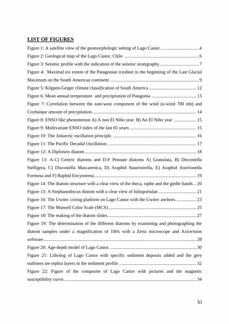

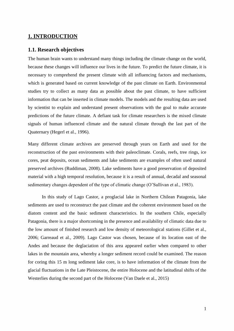


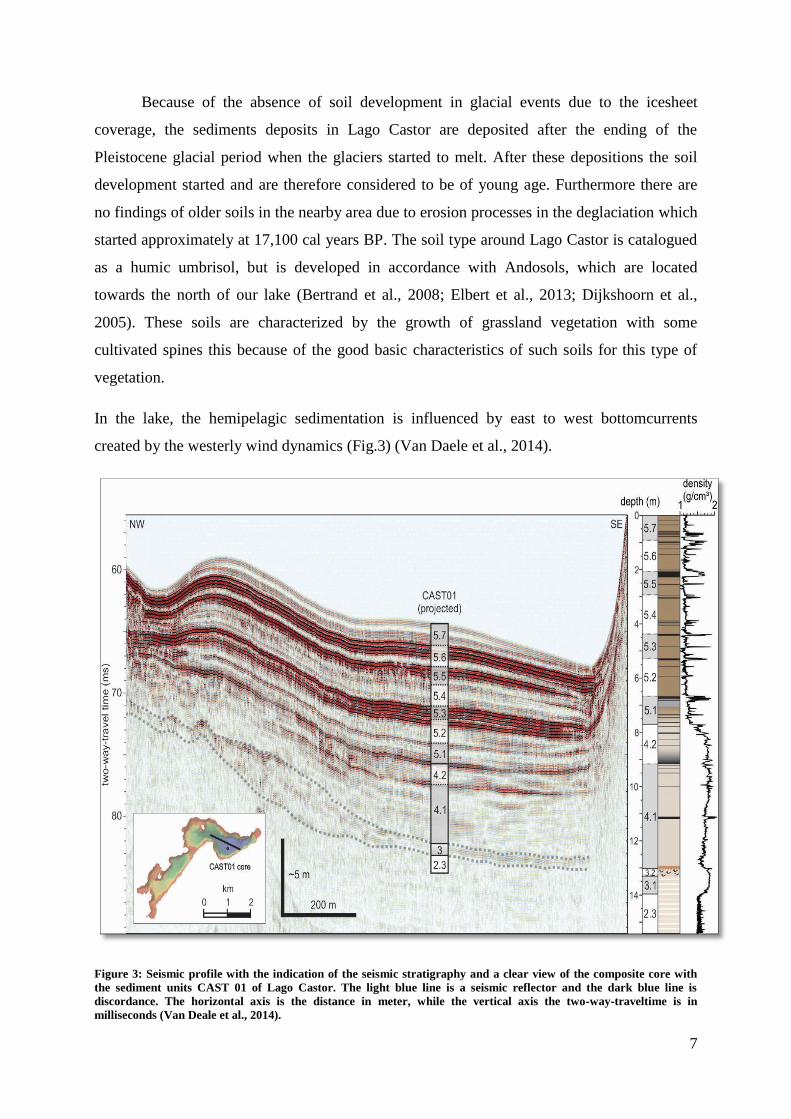


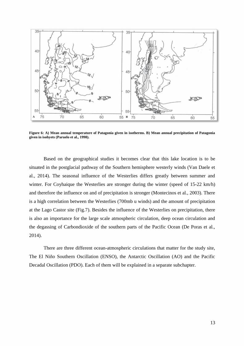
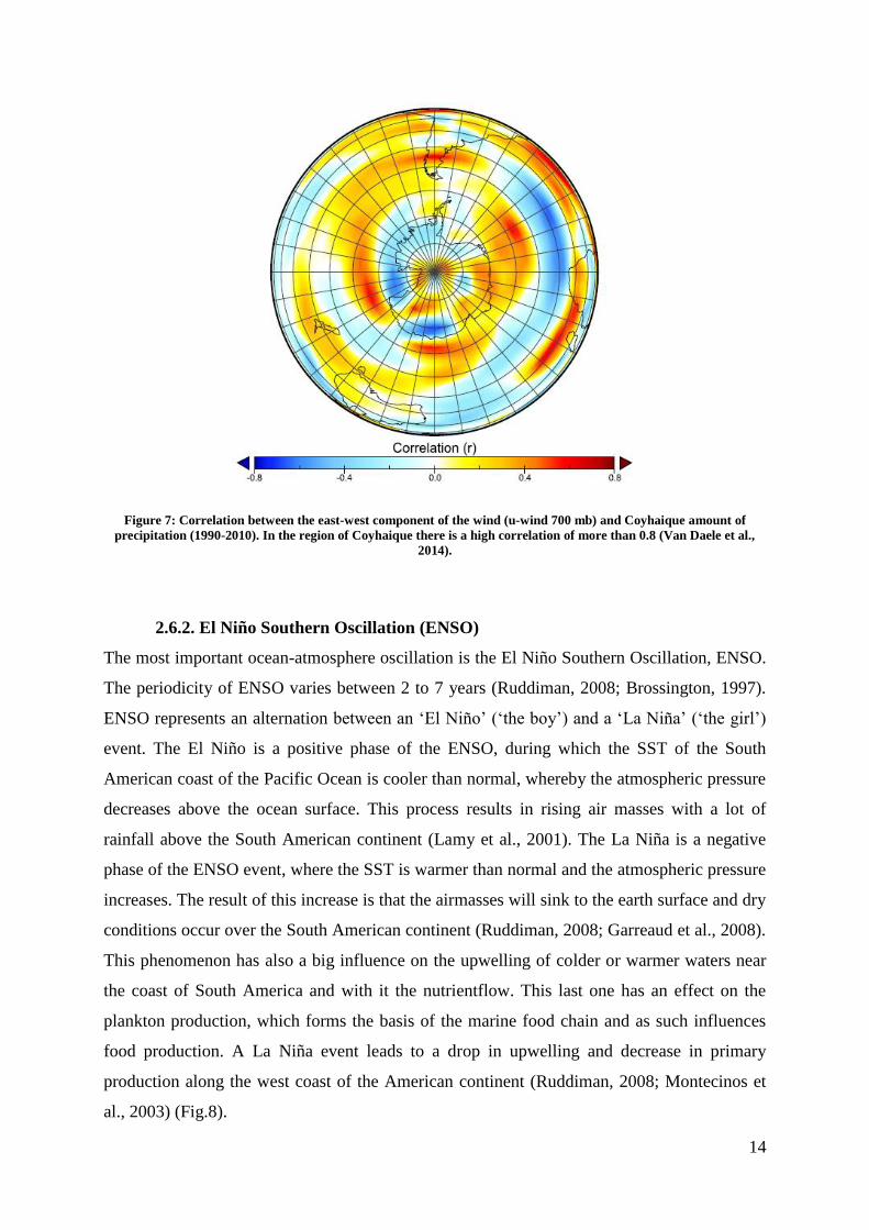

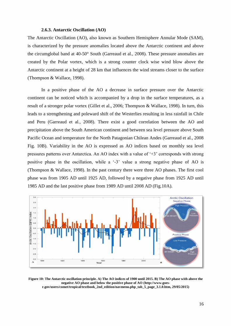


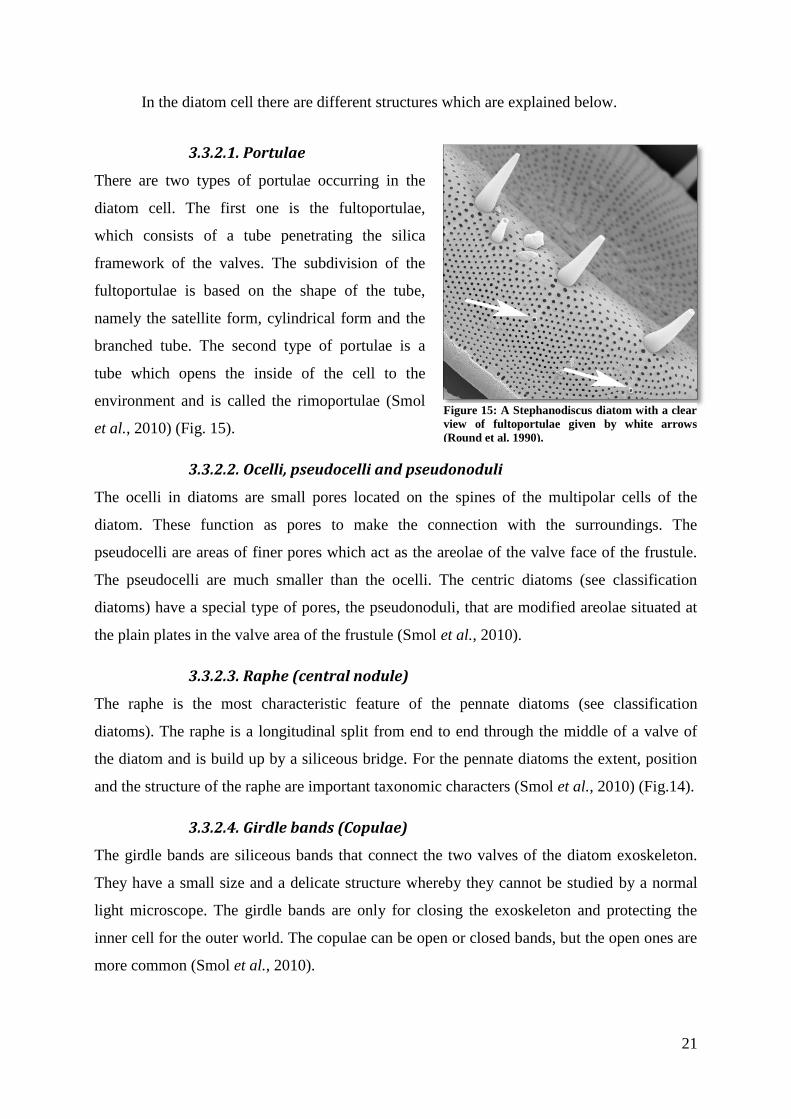


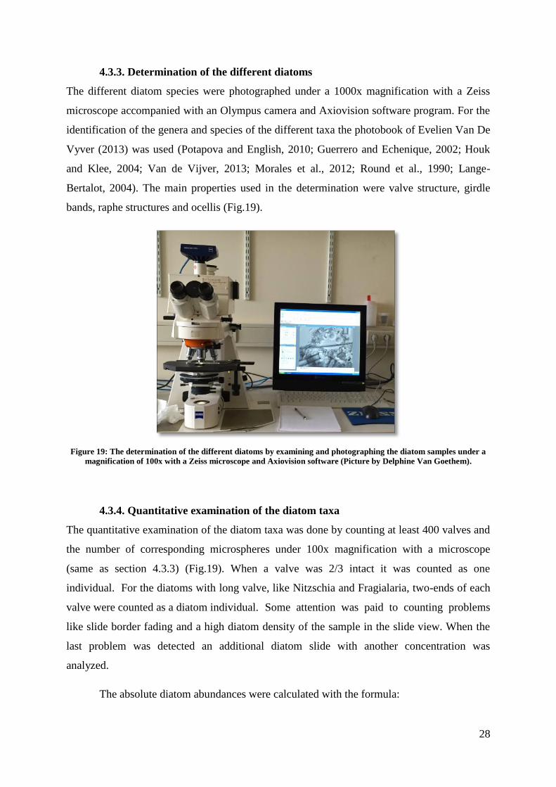


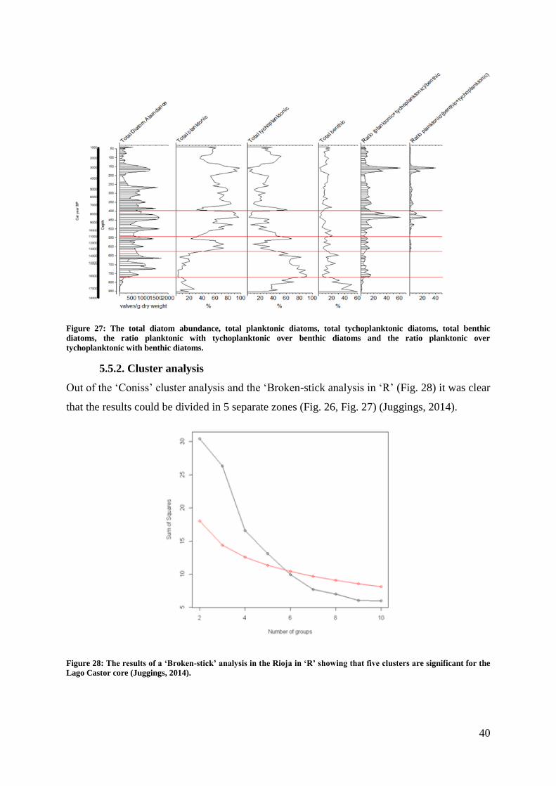
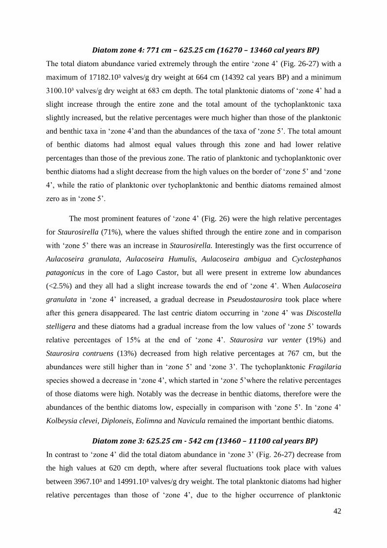


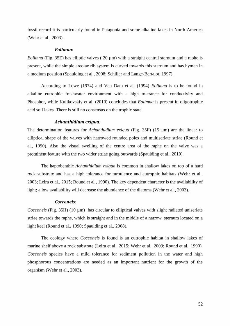


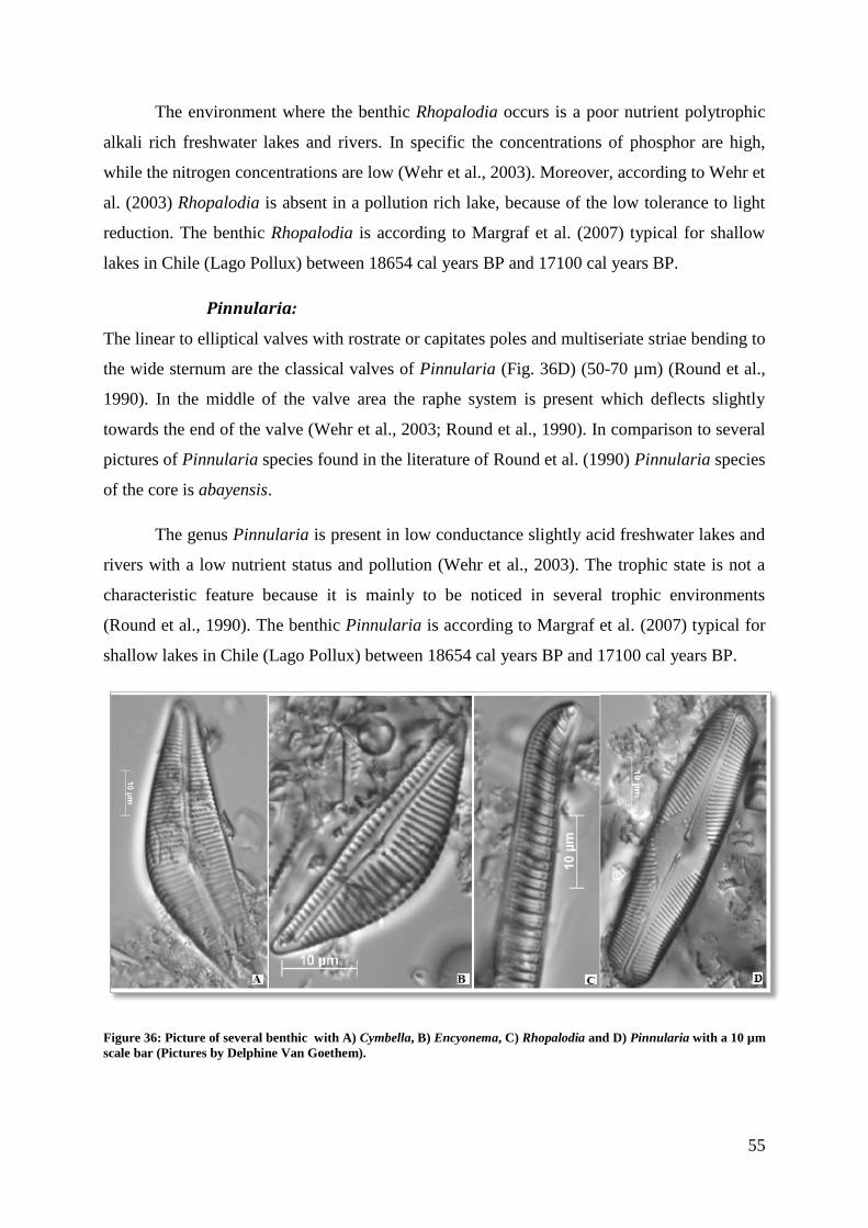
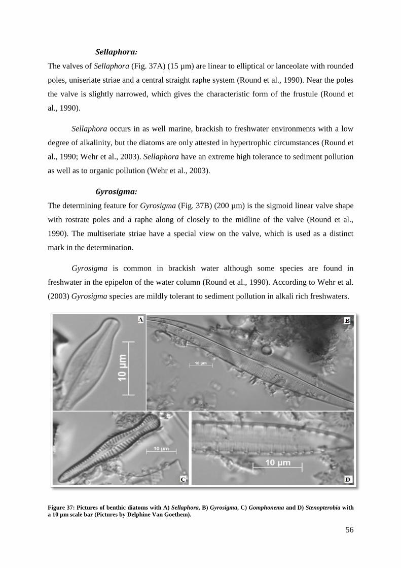


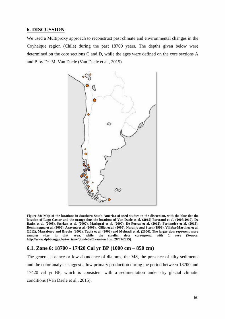


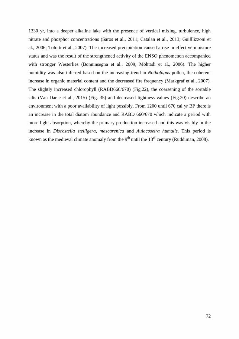


![Flash - Online Coach / eCoach4u...Communicatieadviseur, Copywriter, D], Web-developer. Artistiek Praktisch Creatief beroep waarbij originaliteit, kunst, cultuur of vindingrijkheid](https://static.documents.pub/doc/80x56/5f1069057e708231d448f923/flash-online-coach-ecoach4u-communicatieadviseur-copywriter-d-web-developer.jpg)


