A Differential Geometric Approach to Multiple View Geometry …sastry//pubs/OldSastryALL/Ma... ·...

A Differential Geometric Approach to Multiple ViewGeometry in Spaces of Constant Curvature

Yi MaElectrical & Computer Engineering DepartmentUniversity of Illinois at Urbana-Champaign1406 West Green Street, Urbana, IL 61801Tel: (217)-244-0871 Email: [email protected]

December 11, 2001

Abstract. Based upon an axiomatic formulation of vision system in a general Riemannianmanifold, this paper provides a unified framework for the study of multiple view geometryin three dimensional spaces of constant curvature, including Euclidean space, spherical space,and hyperbolic space. It is shown that multiple view geometry for Euclidean space can be inter-preted as a limit case when (sectional) curvature of a non-Euclidean space approaches to zero.In particular, we show that epipolar constraint in the general case is exactly the same as thatknown for the Euclidean space but should be interpreted more generally when being appliedto triangulation in non-Euclidean spaces. A special triangulation method is hence introducedusing trigonometry laws from Absolute Geometry. Based on a common rank condition, wegive a complete study of constraints among multiple images as well as relationships among allthese constraints. This idealized geometric framework may potentially extend extant multipleview geometry to the study of astronomical imaging where the effect of space curvature is nolonger negligible, e.g., the so-called “gravitational lensing” phenomenon, which is currentlyactive study in astronomical physics and cosmology.

Keywords: Multiple view geometry, spaces of constant curvature, gravitational lensing, epipo-lar constraint, multilinear constraint, algebraic and geometric dependency, triangulation.

1. Introduction

Classic multiple view geometry in a three dimensional Euclidean space ��

(�� with its standard inner product as metric) has been extensively studiedfor the past two decades. A commonly adopted mathematical model for apin-hole camera can be described as:

�� (1)

In this equation, � � �� (the group of �� real matrices of determinant1) is the so-called calibration matrix, � � �� is a standard projectionmatrix, and �� is a homogeneous representation for a Euclideanmotion (denoted by ��) with a rotation �� (the group of�� rotation matrices of determinant 1) and a translation � �� w.r.t. the

c� 2001 Kluwer Academic Publishers. Printed in the Netherlands.

IJCV_kluwer.tex; 11/12/2001; 12:59; p.1

2 Yi Ma

coordinate frame at time � � �:

� �

��

��

��

��

�� (2)

Then �� is the image at time � (in ho-

mogeneous coordinates) of a point � � ��

� (also in ho-mogeneous coordinates). Apparently, � differs from �� by an arbitrarypositive scalar �� . In the literature, sometimes the above equation iswritten as:

��

The fundamental problem for multiple view geometry is then to study howto recover from multiple images �� of a set of points: the camera motion�� and the 3-D coordinates of the points ��.

A widely adopted approach to study this problem is a three-stage stratifica-tion through a projective and then an affine reconstruction (Faugeras, 1995).That is, instead of directly dealing with the Euclidean motion group ��,one introduces two intermediate cases where �� is modified by a projec-tive transformation �� in the group �� or an affine transformation ��in �� .� Respectively, the camera model (1) becomes:

��

or �� (3)

Multiple view geometry for these two camera models has been well estab-lished in the literature (see (Faugeras, 1995; Hartley and Zisserman, 2000)for details). Exercising the same philosophy, we here may further consider amore generalized camera model:

�� (4)

where �� belongs to � which could be any (Lie) subgroup embedded in�� . The reader should be aware that there is a difference between thismodel (4) and the above stratification model (3). For (4), the transformationfrom one camera frame to another can be an arbitrary element in �. Butfor (3) there is essentially only one global projective or affine transforma-tion which acts on all camera coordinate frames simultaneously. Betweencamera frames the transformation is typically not a free projective or affinetransformation.

Certainly, the Euclidean group �� and affine group �� are twocandidates for such �. However, as we will soon see, there are other sub-groups embedded in �� which are not necessarily subgroups of �� nor ��. It is then important to quest:

IJCV_kluwer.tex; 11/12/2001; 12:59; p.2

A Differential Geometric Approach 3

(i) Whether these groups (other than ��) also represent meaningfulvision problems? Are these problems of any practical applications?

On the other hand, conceptually there is obvious limitation for all threegroups �� and �� : they only allow us to study visionin linear spaces (Euclidean �

� or Projective ��) in which light rays travel

straight lines. Hence, multiple view geometry developed so far is based on adefault assumption: the underlying space is essentially a Euclidean space �� .Mathematically, it is then natural to ask:

(ii) If the Euclidean assumption on the underlying space is removed, canwe still study vision or multiple view geometry, and how?

In order to answer this question, we need clearly understand what are all thehidden assumptions which have essentially enabled the development of mul-tiple view geometry so far and how these assumptions can be re-formulatedin a more general form so as to accommodate cases of non-Euclidean spaces.

In this paper, we attempt to provide a definite answer to questions (i)and (ii), which are two questions in fact deeply related. Basically, we willshow that, under certain assumptions, it is possible to generalize multipleview geometry to non-Euclidean spaces by choosing for � in the model (4)subgroups of �� other than �� and �� . From this group the-oretic viewpoint, most results that we have obtained for the Euclidean spacehave their natural extensions to the non-Euclidean case. The Euclidean case inprinciple can be interpreted as an extreme case of the non-Euclidean multipleview geometry. We hope that such a generalization not only captures essentialgeometric characteristics of any imaging system but also provides a unifiedmathematical framework in which we may gain a deeper understanding ofunderlying principles of multiple view geometry in general.

This paper aims to provide a theoretic treatment of multiple view ge-ometry from a differential geometric point of view. Since the geometry ofnon-Euclidean spaces is a well established subject (Kobayashi and Nomizu,1996; Wolf, 1984), we here try not to over address it and only to take whateverresults available to serve our own purpose. Although main techniques in thispaper involve only linear algebra and matrix (Lie) groups, a background indifferential geometry (especially in Riemannian geometry and Lie groups)will certainly improve your appreciation of some general concepts and specialsubjects to be introduced below. Now that we are developing a multiple viewgeometry for non-Euclidean spaces in parallel to that known for Euclideanspace, references for relevant facts for the Euclidean case will be given alongthe development. In case we miss, we point the reader to the book (Hart-ley and Zisserman, 2000), which gives a rather complete and comprehensivesummary of Euclidean multiple view geometry.

IJCV_kluwer.tex; 11/12/2001; 12:59; p.3

4 Yi Ma

2. Vision and Imaging in Riemannian Manifolds

Not until Einstein’s theory of general relativity, non-Euclidean geometry, orRiemannian geometry in general, is more of a pure mathematical creationrather than a geometry of physical meaning. According to general relativity,any physical space is in fact described by a Riemannian manifold and itscurvature is attributed to the distribution of mass in the space. In such a space,light travels the so-called geodesic, i.e. the curve of minimal distance amongall those connecting two given points. Such a curve is in general “bent” bythe field of gravity. If the density of mass is small, the space has almost zerocurvature hence can be approximately assumed to be a Euclidean space �� .Geodesics in this space are then nothing but the straight lines.

2.1. GRAVITATIONAL LENSING

The effect of non-zero space curvature on astronomical imaging has only re-cently been demonstrated by modern deep space telescopes, e.g., the Hubbletelescope.� Below is an example image released by NASA:�

Figure 1. Explanation: Gravity can bend light. Almost all of the bright objects in this HubbleSpace Telescope image are galaxies in the cluster known as Abell 2218. The cluster is somassive and so compact that its gravity bends and focuses the light from galaxies that liebehind it. As a result, multiple images of these background galaxies are distorted into faintstretched out arcs - a simple lensing effect analogous to viewing distant street lamps through aglass of wine. The Abell 2218 cluster itself is about 3 billion light-years away in the northernconstellation Draco.

This phenomenon is referred to as “gravitational lensing” in astronomicalphysics or cosmology. Illustratively, it can be explained by Figure 2.� Thereare a vast body of literature and images on gravitational lenses, for examplesee (Schneider, Ehlers and Falco, 1992).

IJCV_kluwer.tex; 11/12/2001; 12:59; p.4


Figure 2. Albert Einstein predicted that the gravitational field of a massive galaxy would bendlight traveling to Earth from distant quasars. This is what is called “gravitational lensing”,since the intervening galaxy acts as a lens to focus the image of the distant quasar to a newlocation. Gravitational lensing can produce multiple images, rings, or arcs, depending on thedistribution of mass in the galaxy and the Earth-galaxy-quasar geometry.

2.2. AN AXIOMATIC FORMULATION

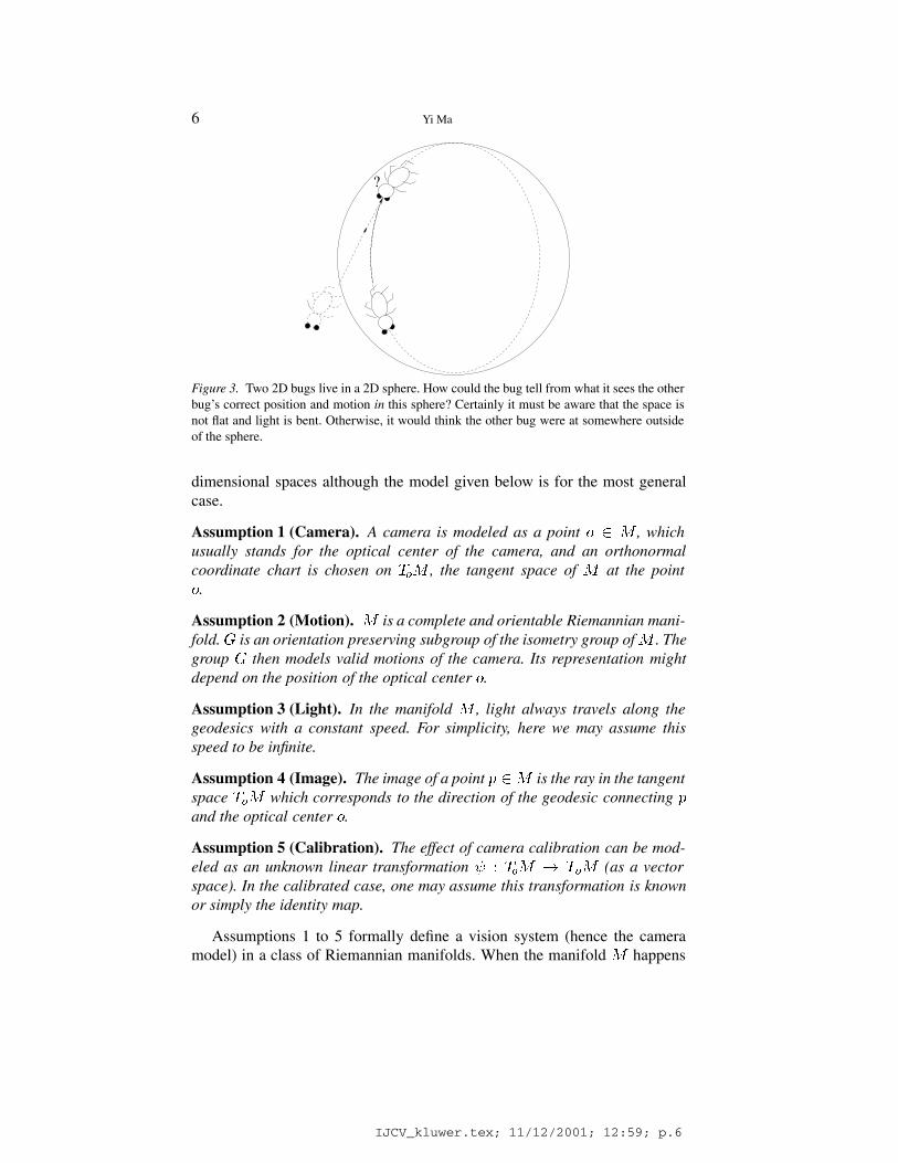
In this paper, instead of studying the physical nature of gravitational lensingin real-world scenarios, we will however consider a more idealistic situation.The idealization will essentially allow us to gain a clear understanding ofgeometric laws which govern imaging and vision in any space of non-zerocurvature. Now, out of curiosity, let us first imagine an intelligent creatureliving in a sphere �

� as illustrated in Figure 3 – the simplest ideal exampleof a 2 dimensional non-Euclidean space with a constant curvature. Unlikein a Euclidean space, light now travels great circles of the sphere instead ofstraight lines. Then what kind of multiple view geometry the creature wouldhave developed? To answer this question, we need to put ourselves in theshoes of this creature and try to understand what are the basic elements thata vision system in such a space must consist of. In this section, we give anaxiomatic formulation of these basic elements. Although the proposed math-ematical model seems to be given in a rather abstract manner, it is indeeda natural generalization of the conventional camera model in the Euclideanspace �� . Such a generalization allows us to fully discover the geometricnature of any vision system in a very concise and precise way, as we will seein later sections.

Let us consider a (connected) Riemannian manifold �� , i.e. a dif-ferentiable manifold equipped with a positive definite symmetric 2-form as its metric. If the reader is not familiar with differential geometry, he orshe may simply replace �� by the Euclidean space �� with its standardinner product metric. In this paper, we will be mostly interested in three

IJCV_kluwer.tex; 11/12/2001; 12:59; p.5

6 Yi Ma

?

Figure 3. Two 2D bugs live in a 2D sphere. How could the bug tell from what it sees the otherbug’s correct position and motion in this sphere? Certainly it must be aware that the space isnot flat and light is bent. Otherwise, it would think the other bug were at somewhere outsideof the sphere.

dimensional spaces although the model given below is for the most generalcase.

Assumption 1 (Camera). A camera is modeled as a point � � � , whichusually stands for the optical center of the camera, and an orthonormalcoordinate chart is chosen on �� , the tangent space of � at the point�.

Assumption 2 (Motion). � is a complete and orientable Riemannian mani-fold. � is an orientation preserving subgroup of the isometry group of � . Thegroup � then models valid motions of the camera. Its representation mightdepend on the position of the optical center �.

Assumption 3 (Light). In the manifold � , light always travels along thegeodesics with a constant speed. For simplicity, here we may assume thisspeed to be infinite.

Assumption 4 (Image). The image of a point � �� is the ray in the tangentspace �� which corresponds to the direction of the geodesic connecting �and the optical center �.

Assumption 5 (Calibration). The effect of camera calibration can be mod-eled as an unknown linear transformation � �� (as a vectorspace). In the calibrated case, one may assume this transformation is knownor simply the identity map.

Assumptions 1 to 5 formally define a vision system (hence the cameramodel) in a class of Riemannian manifolds. When the manifold � happens

IJCV_kluwer.tex; 11/12/2001; 12:59; p.6


to be the Euclidean space �� , the so obtained model is exactly equivalent

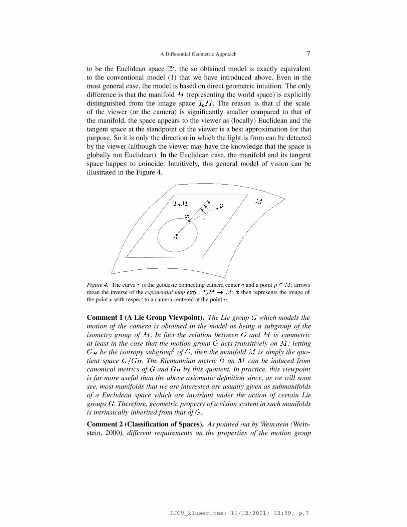
to the conventional model (1) that we have introduced above. Even in themost general case, the model is based on direct geometric intuition. The onlydifference is that the manifold � (representing the world space) is explicitlydistinguished from the image space �� . The reason is that if the scaleof the viewer (or the camera) is significantly smaller compared to that ofthe manifold, the space appears to the viewer as (locally) Euclidean and thetangent space at the standpoint of the viewer is a best approximation for thatpurpose. So it is only the direction in which the light is from can be detectedby the viewer (although the viewer may have the knowledge that the space isglobally not Euclidean). In the Euclidean case, the manifold and its tangentspace happen to coincide. Intuitively, this general model of vision can beillustrated in the Figure 4.

�

��

�

�

�

Figure 4. The curve � is the geodesic connecting camera center � and a point � �� ; arrowsmean the inverse of the exponential map �� ; � then represents the image ofthe point � with respect to a camera centered at the point �.

Comment 1 (A Lie Group Viewpoint). The Lie group � which models themotion of the camera is obtained in the model as being a subgroup of theisometry group of � . In fact the relation between � and � is symmetricat least in the case that the motion group � acts transitively on � : letting�� be the isotropy subgroup� of �, then the manifold � is simply the quo-tient space �� . The Riemannian metric on � can be induced fromcanonical metrics of � and �� by this quotient. In practice, this viewpointis far more useful than the above axiomatic definition since, as we will soonsee, most manifolds that we are interested are usually given as submanifoldsof a Euclidean space which are invariant under the action of certain Liegroups �. Therefore, geometric property of a vision system in such manifoldsis intrinsically inherited from that of �.

Comment 2 (Classification of Spaces). As pointed out by Weinstein (Wein-stein, 2000), different requirements on the properties of the motion group

IJCV_kluwer.tex; 11/12/2001; 12:59; p.7

8 Yi Ma

� may determine the type of manifold that � must be. For example, if werequire � act transitively on the frame bundle� of � , it can be shown that �must be spaces of constant curvature (Kobayashi and Nomizu, 1996). A lessrestrictive requirement on � is to allow that the optical axis of the camera canpoint to any direction at any point of � (but the camera may not be able torotate arbitrarily around the axis). In this case, � corresponds to the so-callsymmetric spaces of rank 1. One can further relax the Assumption 2 so that �does not have to be a subgroup of the isometry group of � . Then � can beany Riemannian manifold. Little is known how to study geometric propertiesof symmetric spaces from a vision point of view much less for Riemannianmanifolds in general. Vision theory for general Riemannian manifolds is outof the scope of this paper. For the remaining of this paper, we will focus onlyon the spaces of constant curvature and demonstrate how to generalize theextant multiple view geometry for Euclidean space to those non-Euclideanspaces.

3. Multiple View Geometry in Spaces of Constant Curvature

Can the abstract model introduced in the preceding section be of any use?In this section we will demonstrate that, using this model, one can actuallyextend extant multiple view geometry developed for the Euclidean space to alarger class of spaces: the spaces of constant curvature. In particular, we willshow that the epipolar geometry has no peculiar meaning to Euclidean space.It is also true for more general spaces. In a similar fashion, dependency amongmultilinear constraints can be uniformly established for the entire class ofspaces of constant curvature.

Spaces of constant curvature are Riemannian manifolds with constant sec-tional curvature. In differential geometry, they are also referred to as ba-sic space forms. A Riemannian manifold of constant curvature is said tobe spherical, hyperbolic, or flat (or locally Euclidean) as the sectional cur-vature is positive, negative, or zero, respectively. See Figure 5. Geometry

�

�

�

Euclidean Spherical HyperbolicFigure 5. Three basic space forms: Euclidean, spherical and hyperbolic. Conventionally onlymultiple view geometry in the first type of spaces has been studied.

IJCV_kluwer.tex; 11/12/2001; 12:59; p.8


about spaces of constant curvature is also called absolute geometry, namedby one of the co-founders of non-Euclidean geometry: Janos Bolyai (Hsiang,1995). For the rest of this paper, we will try to develop a vision theory forthese spaces, as a natural generalization of the extant vision theory for 3dimensional (3-D) Euclidean space. More specifically,

We try to identify all the geometric relationships (or laws) that governmultiple images of an object in a space of constant curvature, from whicha reconstruction of the object and camera locations can be achieved.

We will focus on 3 dimensional spherical and hyperbolic spaces since theEuclidean case has been well understood. On the other hand, as shown inAppendix A, the Euclidean case can always be viewed as a limit case of thegeneral theory.

3.1. HOMOGENEOUS REPRESENTATION OF SPACES OF CONSTANT

CURVATURE

Geometric properties of � dimensional spaces of constant curvatures havebeen well studied in differential geometry (as an important case of symmetricspaces), e.g., see (Kobayashi and Nomizu, 1996). In the rest of this section,we briefly review some of the main results which serve for our purposes. Themain goal is to establish necessary mathematical basis for the derivation ofthe projection model (23) in the next section. However, if the reader is notfamiliar with differential geometry or Lie groups, this section (i.e. Section3.1) can be skipped at first read as long as the reader is willing to take forgranted the three propositions developed in this section and later the cameramodel (23) as a result of them.

The first proposition which characterizes the 3 dimensional space of con-stant curvatures follows directly from a more general statement about � di-mensional spaces, see Theorem 3.1 in Chapter V of (Kobayashi and Nomizu,1996) :

Proposition 1 (Three Dimensional Spaces of Constant Curvature). Let��

� be the coordinate system of �� and � be the hyper-surfaceof �� defined by:

�� (�: a nonzero constant). (5)

Let � be the Riemannian metric of � obtained by restricting the followingsecond order differential form to � : �� . Then:

1. � is a 3 dimensional space of constant curvature with sectional curva-ture ��.

2. The group � of linear transformations of �� leaving the quadratic form�� invariant acts transitively on � as the group ofisometry of � .

IJCV_kluwer.tex; 11/12/2001; 12:59; p.9

10 Yi Ma

3. If � � �, then � is isometric to a sphere of a radius��. If � � �, then

� consists of two mutually isometric connected hyperbolic surfaces in�� , each of which is diffeomorphic to �� .

Now let � be the � � � matrix associated to the quadratic form defining

� : � �

��

�. The isometry group � of � is given as a subgroup of

�� that preserves this quadratic form:

� ��

��

��

Any element � � � then has the form:

� �

��

��

�� (6)

with � � �� and the conditions:

� �� (7)

The isotropy group �� of � which leaves the origin of a coordinate frame(or usually the center of the camera frame) � � �� fixed isisomorphic to the orthogonal group ��:�

��

� ��

��

��

� (8)

As we have discussed before, the manifold � can then be identified with thequotient space �� .�

It follows that the Lie algebra � of the group � (as a Lie group) is the setof the matrices of the form:

�

�! "#� �

��

�� (9)

where ! � �� " � �� and # � �� satisfy the conditions:

!� � ! � � "� �# � �� (10)

Let � be the linear subspace of the Lie algebra � of � consisting of matrices

of the form:�

� "#� �

�� with " # � �� and " � �# � �. Let � be the

Lie algebra of �� as a subspace of � which consists of matrices of the form:�! ��

�� with ! � �� and !� � ! � �. Then we have a canonical

decomposition:

� � ��

IJCV_kluwer.tex; 11/12/2001; 12:59; p.10


It is direct to check the following relations between the subspaces hold:

�� (11)

where �� stands for Lie bracket.� Let � be the vertical tangent subspaceof � and � be the horizontal tangent subspace. Then according to Theorem11.1 in Chapter II of Kobayashi (Kobayashi and Nomizu, 1996), this decom-position gives a canonical connection on the principle bundle �� which in turn induces constant sectional curvature �� on �� .

The canonical decomposition of the Lie algebra � of � results in a de-composition of the group � into two basic actions. One is the rotation arounda fixed point, characterized by the subgroup �� or the subalgebra �; theother is the translation along geodesics of the manifold � which is obviouslyrelated to the subalgebra �. Denote the quotient map from � to �� as$ � � �� . Let � �� be the exponential map from � to �.�� Thenaccording to Theorem 3.2 in Chapter XI of (Kobayashi and Nomizu, 1996),we have:

Proposition 2 (Characterization of Geodesics). Consider the three dimen-sional space of constant curvature �� as above. For each % � �,$�� %�� %� � � is a geodesic starting from � and, conversely,every geodesic from � is of this form.

Now let �� be the subset of � consisting of all the matrices of the form� ��%� with % � �:

�� %� � �

�� % � �� (12)

Then �� corresponds to the so-called transvection on � , an analogy totranslation in the Euclidean space. Notice that in general �� is not a sub-group of � (although it is in the Euclidean case) since its representationdepends on the base point �. On the other hand, the isotropy subgroup �� of� corresponds to rotation on � . As in the Euclidean case, for a “rigid bodymotion” on � , it is natural to consider the rotation is in the special orthogonalgroup �� instead of the full orthogonal group ��. One of the reasonsfor only considering �� is that it preserves the orientation of the space.

First notice that, as in the Euclidean case, the transvection set �� of theisometry group � acts transitively on a space � of constant curvature.��

Then for any � � �, there exists �� such that �� , i.e.�� fixes the origin �. So �� , the isotropy group of �. We call thiselement �� . It then follows that the group � is equal to:

� � �� (13)

This is the so-called Cartan decomposition. Hence for any motion � � � inthe space � , it can always be written as the (matrix) product of a transvection

IJCV_kluwer.tex; 11/12/2001; 12:59; p.11

12 Yi Ma

�� and a rotation ��:

� � �� (14)

where �� is of the form (8). We now determine the general expression for�� %�.

According to Proposition 2, any geodesic connecting a point � � ��

� �� to the origin � has the form: � � � ��%� � � for some % � �.Without loss of generality, we may assume that % has the form:

% �

�� "

"� ��

��

�� (15)

for some vector " � �� . To simply the notation, define & � " and a vector

� � "�& � �� of unit length. Here, we use the notation � to represent

a translational (or more precisely, transvectional) vector. We may extend thefunctions �� and �� to analytic functions defined on the entire complexplane � :

��'� ��

�(�)� )�� '� �

�

��)� � )�� ' � � � (16)

Also define * �� . Then through direct calculation of the exponen-

tial of the matrix % , we get:

� ��%� �

��

��

�� &*� �� *�� &*��

* ��&*�� &*�

� (17)

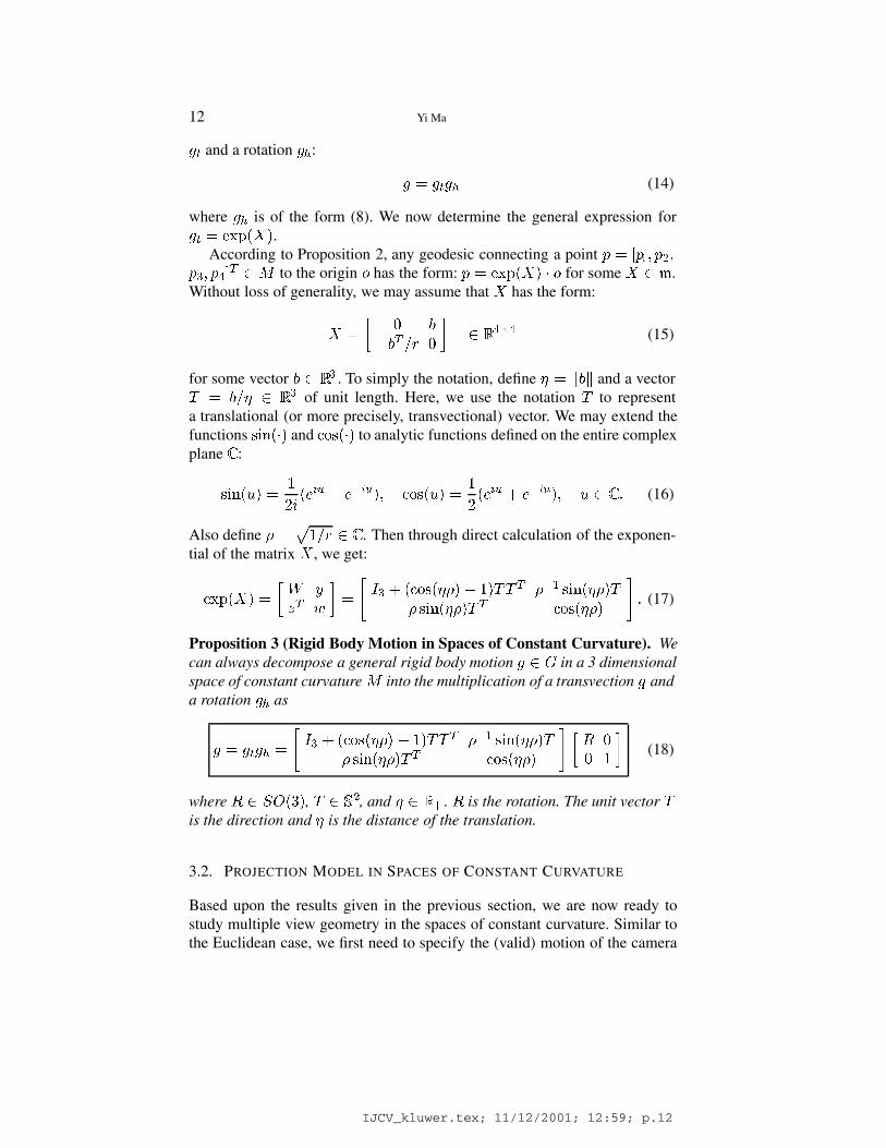
Proposition 3 (Rigid Body Motion in Spaces of Constant Curvature). Wecan always decompose a general rigid body motion � � � in a 3 dimensionalspace of constant curvature � into the multiplication of a transvection �� anda rotation �� as

� � ��

�� &*� �� *�� &*��

* ��&*�� &*�

� ��

�(18)

where � ��, � � ��, and & � �� . is the rotation. The unit vector �is the direction and & is the distance of the translation.

3.2. PROJECTION MODEL IN SPACES OF CONSTANT CURVATURE

Based upon the results given in the previous section, we are now ready tostudy multiple view geometry in the spaces of constant curvature. Similar tothe Euclidean case, we first need to specify the (valid) motion of the camera

IJCV_kluwer.tex; 11/12/2001; 12:59; p.12


and the projection model of the camera, i.e. how a 2 dimensional image isformed in spaces of constant curvature. Basically, we will formally establishthe fact that the camera model for a three dimensional space � of constantcurvature does fit in the general camera model (4) introduced before:

�� (19)

where �� is a rigid body motion on � as explicitly represented by Proposi-tion 3.

A point �, in a space � of constant curvature, can be represented inhomogeneous coordinates as � � ��

� � �� which satisfies thequadratic form: �� with �� the sectional curvature of� . Then under the motion �� of the camera, thehomogeneous coordinates of the point � (with respect to the camera frame)satisfy the transformation:

�� (20)

Notice that, with this representation, the point � � �� is alwaysin � . We then call the point � the origin of � . Without loss of generality,this origin is always identified with the center of the camera. So when theorigin moves, the coordinates of any point � in � change according to (20).

Now consider the geodesic connecting the origin � � �� to �.According to Propositions 2 and 3, we have:

� � � ��%� � � �

�� &*� �� *�� &*��

* ��&*�� &*�

��

��

�*�� &*��

��&*�

��

� � (21)

Therefore, the unit vector � is equal to:

� ��

��

� ��

This is exactly the unit tangent vector of � at the origin � pointing in thedirection of the point �. Or in other words, the geodesic connecting the originto the point � � ��

� � � has its tangent vector at the origin as� � �� given in the above.

Combining Assumption 4 and the above discussion, the image of a point� at time � can then be any vector � � �� on the ray �+� � + � ��.Therefore, in homogeneous coordinates, the image � of the point � differsfrom the vector ��

� by an unknown scalar � � �� . Still

IJCV_kluwer.tex; 11/12/2001; 12:59; p.13

14 Yi Ma

define the standard projection matrix � � �� as before. We then

have the relationship:

�� (22)

We call the scalar �� the scale of the point � with respect to the image ��at time �. � is different from & which is exactly the geodesic distance from �to �. They are related by

� � *�� &*��

Then both the scale � and & encode the depth information of the point �.Furthermore, if the calibration of the camera is unknown, the transformation� �� in Assumption 5 can be represented by a non-singular� � � matrix � since �� is isomorphic to �

� as a vector space. Then theabove model for the camera is modified to:

�� (23)

where �� is a rigid body motion on � (as we have claimed inthe beginning of this section).

3.3. GEOMETRY AND RECONSTRUCTION FROM PAIRWISE VIEWS

In this section, we study the relationship among two images of a point � �� subject to a rigid body motion of a camera in a space � of constantcurvature. According to the Cartan decomposition (Proposition 3), we knowthat a rigid body motion of the camera can always be expressed in the form:� � �� . The transvection part �� and rotation part ��respectively have the forms:

�� %� �

��

� ��

� ��

� (24)

where % � � � �� and expressions for � � ��

and � � � are given by (17). Then the projection model (23) becomes

�� (25)

3.3.1. Epipolar Constraints in Spaces of Constant CurvatureWe first assume that the camera is calibrated, i.e. � � ��. Denote the imagesof � � ��

� before and after a rigid body motion � as ��

and �� , respectively. Then according to (23) or the equation above wehave: �� and �� . They yield:

��

�� (26)

IJCV_kluwer.tex; 11/12/2001; 12:59; p.14


We in this paper use �' to denote the skew symmetric matrix associated to avector ' � �� such that �', � '� , for any , � �� .

In the Euclidean case, (26) would exactly give the well-known bilinearepipolar constraint. As noticed, in the general case, the role of essential matrixis replaced by ��. We need to study the structure of this matrix. Accordingto (17), we have:

� � �� &*� �� *�� &*�� (27)

Notice that we always have �� . Suppose ��&*� �� . Then (26)yields:

��

�� &*� ��

�� (28)

This is exactly the well-known bilinear epipolar constraint. Here we see thatthis constraint holds for all spaces of constant curvature. The same as in theEuclidean case, we call � �� the essential matrix. As a summary of theabove discussion, we have the following theorem:

Theorem 1 (Calibrated Epipolar Constraint). Consider a rigid body mo-tion of a camera in a space � of constant curvature. If � � �

� is the vectorassociated to the direction of the translation and � �� the rotation,then the images �� and �� of a point � �� before and after themotion satisfy the epipolar constraint:

�� (29)

Corollary 1 (Uncalibrated Epipolar Constraint). If the camera has an un-known calibration described by a non-singular matrix � � �� , the epipo-lar constraint in the above theorem becomes:

��

�� (30)

The matrix - � �� is called fundamental matrix as in the Eu-clidean case.

In the Euclidean case, the epipolar constraint essential states the fact thatthe two optical centers and the 3-D point � being observed are coplanar. An-other way to say this is that these three points form a triangle, which in turndetermines a plane. Then in the more general cases, the epipolar constraintsimply states the common fact that the two optical centers and the 3-D point� being observed must form a “geodesic triangle”. This is illustrated in Figure6.

IJCV_kluwer.tex; 11/12/2001; 12:59; p.15

16 Yi Ma

��

)�)�

�

��

� � �

��

��

�

Figure 6. Geodesic triangle formed by two optical centers �� and a point � in the scene.�� are the two images of the point �. �� are the corresponding epipoles.

Comment 3 (Periodic Geodesics). The condition ��&*� �� is equivalentto the condition that the translation � �� in the Euclidean case. The reasonis when ��&*� � �, we have � ��%� � ��, i.e. the motion is equivalent tothe identity transformation on � . In spaces of constant curvature, we mayhave ��&*� � � without � � �. This occurs only when the curvature � ispositive, i.e. the space is spherical. If so, let & � �.$

�� . � � � � � � ,

we then have ��&*� � ��.$� � �. This implies that a translation ofdistance �$

�� along the geodesics (big circles) in a spherical space of radius�

� is equivalent to the identity transformation – you travel back to the initialposition by circling around the globe once. One can easily verify this on a 2dimensional sphere �� or a circle ��.

As in the Euclidean case, using the epipolar constraint, the essential ma-trix � �� can be estimated (up to a scale) from more than eight imagecorrespondences �� in general positions using linear ornonlinear estimation schemes. The rotation matrix and the translation vec-tor � can further be recovered from decomposing the essential matrix (see(Ma, Kosecka and Sastry, 1999; Maybank, 1993) for the details). In the un-calibrated case, the fundamental matrix - is first recovered and the unknowncalibration � can be solved from the well-known Kruppa’s equations (Ma,Vidal, Kosecka and Sastry, 1999) or other self-calibration methods.

3.3.2. Triangulation Using Absolute TrigonometryKnowing the motion parameters � � �, the next problem is how to recon-struct the scale information from images, which includes the scale � of thepoint � with respect to its image �, the distance of the translational motionalong � and, if possible, the constant curvature �� of the space � . But wewill soon see, not both the curvature and the scales can be uniquely deter-mined from image measurements. We here first demonstrate the main ideasfor two calibrated images.

IJCV_kluwer.tex; 11/12/2001; 12:59; p.16


To simplify the notation, in this section, we assume that the image � ofa point � is always normalized, i.e. � � � (in the Euclidean case, thiscorresponds to the so-called spherical projection). Suppose the distance from� to the optical center � is & � �� . Then the homogeneous coordinate of � isgiven in terms of � and & by:

� �

�*�� &*��

��&*�

��

� � (31)

Consequently, the scale � of � with respect to � is given by � � *�� &*�.To differentiate from the scale �, the distance quantity & will be called thedepth of the point � with respect to the image �.

Let &� and &� be the depths of the point � with respect its two images�� and �� taken by the camera at two positions, respectively. Suppose thecamera motion � � � is specified by the rotation � ��, the transla-tion direction � � �

� and the distance of translation � (as in the precedingsection). Then the first equation in (26) yields:

*�� &�*�� *� ��

�*�� &�*��

��&�*�*�� *�� (32)

This is the coordinate transformation formula in spaces of constant curva-ture.

Comment 4. Although seemingly a little complicated, the above equation isno more than a natural generalization of the Euclidean coordinate transfor-mation formula which people are familiar with. Notice that when the curva-ture �� goes to zero, so does * �

��. Since

��

��&�*� � � ��

*�� &�*� � &� (33)

in the Euclidean case (32) simply becomes:

�� (34)

That it, in the limit case, the scale � and the depth & are the same; and theequation (32) gives rise to the familiar Euclidean coordinate transformationformula. Naturally, to reconstruct structure in spaces of constant curvature,the equation (32) has to be exploited instead.

Notice that equation (32) is homogeneous in the scale of *. Since thequantities &� &� and � are all multiplied with *, they can only be determinedwith respect to an arbitrary scale of *. Thus in the case of spaces of con-stant curvature, we may normalize everything with respect to the scale of thecurvature: if � � �, let * � �; if � � �, let * � ( �

��. That is, now

IJCV_kluwer.tex; 11/12/2001; 12:59; p.17

18 Yi Ma

the space � has constant sectional curvature of either �� or �. Then (32)respectively becomes:

��&��

� � ��&��

��&�� * � ��

��&��

� � ��&��

��&�� * � (�

These two equations correspond to coordinate transformations in (normal-ized) spherical and hyperbolic spaces, respectively.

Proposition 4. In a space of constant curvature, the curvature of the space isnot recoverable from multiple images unless the distance between points areknown a priori.

From the preceding section, we know and � can be estimated fromepipolar constraints. The problem left is to reconstruct &� &� and �. Supposethat the two optical centers of the camera are �� and ��. A geodesic triangleis formed by the three points �� , see Figure 7. The angle � is given by

&�&�

�

�

��

�� /

0

Figure 7. Geodesic triangle formed by two optical centers �� and a point � in the scene.For this triangle, we have � � �� and � �.

the angle between the two vectors �� and �� ; / is given by the angle be-tween �� and � . Unlike the Euclidean case, we here cannot directly computethe angle 0 from � / since the sum of ��/�0 is not necessarily $ in thecase of a Riemannian manifold. According to the Gauss-Bonnet Theorem:

��/ � 0 $ � 1 � area��/0� (35)

since here the space has a constant Gauss curvature 1 � �� after normal-ization.

The problem of determining lengths &� &� � from such a triangle is usu-ally referred to as triangulation as in the Euclidean case (Hartley and Sturm,1997). In the Euclidean case, one may directly use above coordinate trans-formation formula (34) to formulate linear least square type of objective

IJCV_kluwer.tex; 11/12/2001; 12:59; p.18


functions for estimating depths & and � (Ma, Kosecka and Sastry, 1999).However, in the non-Euclidean case, such objective functions are much morecomplicated in the unknown & and � for obvious reasons.

In stead of directly solving for all the unknown variables simultaneously,let us first try to identify the minimum number of constraints on such atriangle based on the well-known trigonometry in spaces of constant curva-ture. They are the so-called Bolyai’s law of sine and law of cosine (in thecase of absolute geometry), which are summarized in (Hsiang, 1995). Definefunctions:

2��

�� * � � �� * � (

3��

�� * � � �� * � (�

The next proposition follows from (Hsiang, 1995) as a special case:

Proposition 5 (Laws of Absolute Trigonometry). Consider a geodesic tri-angle ��/0 in a space � of constant curvature ��, and let ! " # be thelengths of the opposite sides of angles � / 0 respectively. Then we have:

1. Bolyai’s law of sine:

��

2�!��

��/�

2�"��

��0�

2�#� (36)

2. Bolyai’s law of cosine:

2�!�2�"� ��0� � 3�#� 3�!�3�"�

2�"�2�#� �� 3�!� 3�"�3�#� (37)

2�#�2�!� ��/� � 3�"� 3�#�3�!��

In our case only the quantities �� /� �� /� in the aboveequations (36) and (37) are known to us. Either the sine law or the cosinelaw gives only two independent algebraic constraints on three unknowns! � &� " � &�, # � �. Hence it is in general impossible to uniquelydetermine &� &� �.�� Like the Euclidean case, this corresponds to the well-known fact that the structure can only be reconstructed up to a universal scale.Hence without loss of generality, we can further normalize the distance � oftranslation such that

2�� or equivalently 3�� (38)

The cosine law gives ��0� � �� /� and so we know ��0�too. Consequently the depths &� &� are given by:

2�&��

��0� 2�&��

��/�

��0�(39)

IJCV_kluwer.tex; 11/12/2001; 12:59; p.19

20 Yi Ma

from the sine law since 2�� .

3.4. GEOMETRY AND RECONSTRUCTION FROM MULTIPLE VIEWS

It is already known that in the Euclidean case, 4 images of a point satisfycertain multilinear constraints besides the bilinear epipolar constraints. Sim-ilar constraints exist in the case of spaces of constant curvature. We heregive a complete study of those constraints through the use of the so-calledrank condition. Relationships among different types of constraints can alsobe easily revealed this way.

Suppose �� ( � � � � � � 4 are 4 images of the same point � with

respect to the camera at 4 different positions (or vantage points). Suppose therelative motion between the (�� and �� positions is �� ( � � � � � � 4.Let �� ( � � � � � � 4 be the scales of � w.r.t. the images �� ( �� 4. Then we have the following equation:��

�� ...

.... . .

...� � � � � ��

��

��...

��

��

��

...��

�� (40)

Let us call the matrix �� as the (�� projection matrix.

Without loss of generality, we may always assume that the first projectionmatrix �� is of the standard form ��

�� .�� In general the (��

projection matrix is of the form:

�� (41)

where � � are given in (27). For simplicity, we call the first three columnsof �� as 5�

�� and the last column as 6�

�� . Now

define a so-called multiple view matrix �� to be

��

��5�� 6��5�� 6�

......��5�� 6�

�� (42)

The superscript ! in �� indicates absolute geometry. Similar to the Eu-clidean case (Ma, et. al., 2001), in spaces of constant curvature, we alsohave:

Theorem 2 (Multiview Rank Condition). Consider 4 images �� of a point � in a space � of constant curvature. The multiple view matrix�� defined above satisfies

� � rank�� (43)

IJCV_kluwer.tex; 11/12/2001; 12:59; p.20


The proof is essentially the same as in the Euclidean case (Ma, et. al.,2001). For the same reasons as in the Euclidean case, it is straightforward tosee that non-trivial constraints given by the above rank condition are eitherbilinear or trilinear in the image coordinates ��’s:��

��6�5�� 6�� 5�

� 5��6�� (44)

As we see, the bilinear type gives exactly the epipolar constraint we derivedbefore (30).

Corollary 2 (Linear Relationships among Multiple Views of a Point). Forany given 4 images corresponding to a point � � � relative to 4 cameraframes, that the matrix �� is of rank no more than � yields the following:

1. Any algebraic constraint among the 4 images can be reduced to onlythose involving � and � images at a time. Formulae of these bilinearand trilinear constraints are given in (44) respectively. There is no otherrelationship among point features in more than three views.

2. For given 4 images of a point, all the triple-wise trilinear constraintsalgebraically imply all pairwise bilinear constraints, except in the degen-erate case in which the pre-image � lies on the geodesic through opticalcenters �� for some (.

It is also easy to see that the kernel of the multiple view matrix �� is

��

��

�� (45)

where �� is exactly the scale of the point � relative to the first camera frame.Hence the multiple view matrix associated to 4 images exactly capturesthe scale (or depth) information (of a point) that is missing in a single im-age but encoded in multiple ones. The kernel of �� is unique except whenrank�� , i.e. �� . The latter corresponds to a rare configurationwhere all camera centers �� and the point � lie on the same geodesic.We hence have the following statement regarding a geometric interpretationof the multiple view matrix:

Corollary 3 (Uniqueness of the Pre-image). Given 4 vectors on the imageplanes with respect to 4 camera frames, they correspond to the same pointin the 3-D space � if the rank of the �� matrix is 1. If its rank is 0, the pointis determined up to the geodesic where all the camera centers must lie on.

This is illustrated in Figure 8. The reader may have been aware that aboveresults are very much consistent with what we have known in multiple viewgeometry for the Euclidean space. The rank conditions on the multiple view

IJCV_kluwer.tex; 11/12/2001; 12:59; p.21

22 Yi Ma

��

&�

��

��

��

��

��

rank�� rank�� Figure 8. Two cases corresponding to the two rank values of ��. Left: a generic case; Right:a degenerate case.

matrix also applies to line or plane features in the Euclidean case. We shouldtherefore expect a similar story holds in the general case. We here omit thedetail for simplicity.

From the above study, we see that the distinction of multiple view geome-try between Euclidean and non-Euclidean spaces is very subtle. They all obeythe same projection model:

�� (46)

except that the internal structure of the projection matrix �� may bedifferent. This has therefore revealed a very interesting and important fact:The same set of parameters for the projection matrices

��

��

��...

��

��

��

......

��

�� (47)

can have different interpretations. They are all geometrically meaningful. Forexample, we know the above � can be interpreted as the projection matricesof an uncalibrated camera with constant calibration � moving in a spaceof constant curvature. It can also be interpreted as an uncalibrated camerawith time-varying calibration �� moving in a Euclidean space. Then �

and �� become the rotation and translation of the camera motion. Hence

essentially

Corollary 4 (Equivalence of Imaging Systems). Taking images of an ob-ject in a non-Euclidean space is equivalent to taking images of (the sameobject) in a Euclidean space (probably at a different set of vantage points) andintroducing on each image an unknown linear transformation that depends onthe vantage point.

IJCV_kluwer.tex; 11/12/2001; 12:59; p.22


According to this, reconstruction of a 3 dimensional scene from multipleimages in general is ambiguous. It only becomes well-conditioned if we havesufficient a priori knowledge on the space, the camera calibration, or thecamera motion.

This extra ambiguity and complexity in recovering the projection ma-trix �� make the problem of obtaining a global recon-struction from multiple images of multiple points much harder in the non-Euclidean case. For instance, conventional projective factorization and strat-ification methods (Hartley and Zisserman, 2000) designed for the Euclideancase no longer apply to the non-Euclidean case even in the simplest case� � � . However, factorization methods based on the above rank condition(43) work just the same, see (Ma, et. al., 2001). We here omit the detail forsimplicity.

4. Extensions and Applications to Spaces of Non-constant Curvature

We all know light travels a path of the shortest distance. However, in general,“a path of the shortest distance” does not necessarily mean a straight line. Forinstance, it is well-known in physics that when light or seismic wave travelsacross inhomogeneous media, its trajectory is bent according to the Snell’slaw of sine, as shown in Figure 9:

� ��7� � constant (48)

where 7 is the incidence angle and � is the index of refraction. � is typ-ically the ratio #�, between the speed of light in vacuum and that in themedia. Figure 9 demonstrates two cases when � is piecewise constant orvaries smoothly. The latter case usually occurs when light travels througha depth of sea water with different mineral density or seismic waves throughthe earth. Geometrically we now know that the reason for such refractioncan be explained as a different distribution of material introduces a different(Riemannian) metric to the space. Such metric in general induces a non-zero(sectional) curvature to the space and makes it no longer Euclidean. Nonethe-less, the light always travels the shortest distance with respect to the newmetric – the Snell’s law simply describes what these shortest distance pathsare in some special cases. Hence the geometric framework developed in thispaper can certainly be used to unify the study of vision and imaging problemsassociated to these phenomena. For instance, restriction of the multiple viewgeometry introduced in this paper to a 2 dimensional spherical space can beused to locate the center of earthquake (on the surface of earth) by observingseismic waves from multiple observation posts far away.

This paper only studies a rather idealistic case when the sectional curva-ture of the space is constant in all directions. Such an idealization undoubtly

IJCV_kluwer.tex; 11/12/2001; 12:59; p.23

24 Yi Ma

1

2

�� 7�

7��

�� 7�� 7�� 7�� constant

normalnormal

Figure 9. Snell’s law of sine. Left: A ray of light travels through two different media; Right: Aray of light travels through a media with an index of refraction � as an increasing continuousfunction of the depth �.

will limit its application to real-world situations. However, it is an importantconceptual step towards any further development of more realistic imag-ing and vision models for non-Euclidean spaces which are of much morepractical importance. For example, in the case of gravitational lensing (seeFigure 2), the earth-galaxy-quasar geometry can be approximated as a spaceof piece-wise constant curvature as shown in Figure 10.

� � � � � ��

earth galaxy quasar

Figure 10. An approximate space model for the earth-galaxy-quasar geometry. Around thelarge galaxy, the space has a non-zero curvature due to the gravitation of a large mass.

As one may have recognized that essentially the camera model for a spaceof non-zero curvature is to allow a non-Euclidean motion (described by thegroup �) from one camera frame to another. A similar scenario arises whenmultiple images of a dynamical scene are considered. Although it is shownin (Kun, Fossum and Ma, 2001) that a dynamical scene can usually be em-bedded in a higher dimensional Euclidean space, the transformation betweenprojection matrices is typically non-Euclidean, which is imposed not by acurvature but by the nature of dynamics in the scene. Therefore, the proposedstudy of the more generalized model (4) other than the conventional ones (3)becomes necessary again when one wants to generalize classic multiple viewgeometry to dynamical scenes.

IJCV_kluwer.tex; 11/12/2001; 12:59; p.24


5. Conclusions

In this paper, we have generalized basic results in multiple view geometryfor Euclidean space to spaces of constant curvature. A uniform treatment ispossible because a unified homogeneous representation of these spaces existsand the isometry groups of these spaces are naturally embedded in �� .Consequently, multiple view geometry for spaces of constant curvature is re-markably similar to that for Euclidean space. In particular, epipolar constraintremains exactly the same and so do conditions for dependency among multi-linear constraints. This allows us to extend most motion recovery algorithmspreviously developed for Euclidean space to spherical and hyperbolic spaceswith little change. As for the triangulation problem, the three dimensionalstructure can only be reconstructed up to a universal scale, the same as theEuclidean case. Moreover, without knowing the scale, the curvature of thespace cannot be recovered from image measurements at all – only its signcan be detected.

When the sectional curvature of a Riemannian manifold in all directions isapproximately the same, it can be locally modeled as one of the space formsstudied in this paper. The multiple view geometry that we have developedmay provide a good approximation to the vision problem in such a manifold.However, it remains a question whether results such as epipolar constraint stillgeneralize to more general classes of Riemannian manifolds (for example,symmetric spaces of rank 1); and how the triangulation method needs to bemodified. At this point, little is known about vision beyond spaces of constantcurvature. It remains an open problem for future investigation.

As we have illustrated before, a general theory of multiple view geometryin general Riemannian manifolds can be useful for seismic or astronomicalpurposes, where typically the curvature of a space can no longer be neglecteddue to either a large scale or a lack of homogeneousness in spatial property.However, there has not yet been much effort to study geometric propertiesof such spaces (or manifolds) from a vision perspective much less we knowabout vision in a space-time where relativity plays a significant role, i.e. whenthe speed of light can no longer be assumed to be infinite. In any case, a largepart of relationships among vision, motion, and space is yet to be investigatedin a more general geometric setting.

IJCV_kluwer.tex; 11/12/2001; 12:59; p.25

26 Yi Ma

Appendix

A. Euclidean Space as a Space of Constant Curvature

Proposition 1 requires the curvature parameter � �� hence only the sphericaland hyperbolic spaces were considered. However, the Euclidean case can beregarded as the limit case when � goes to infinite, i.e. the sectional curvature�� goes to zero.

When � ��, a point in �� which satisfies the quadratic form (5) alwayshas the form ��

� � �� . This is just the homogeneous represen-

tation of the 3 dimensional Euclidean space �� , see (Murray, Li and Sastry,1994). Then the condition (7) has become:

�� (49)

Thus the group � is just the Euclidean group ��. In particular, the specialEuclidean group �� with elements:

� �

� ��

��

��

with � �� and � � �� is an orientation-preserving subgroup of theEuclidean group � � ��. As we already know, �� represents the rigidbody motion in � � �

� .When � � �, the Lie algebra 8)�� of �� or )�� of �� then has

the form given in (9) with the condition # � �. In robotics literature (Murray,Li and Sastry, 1994), an element of this Lie algebra is usually represented astwist:

�

� �9 ,� �

��

��

where 9 , � �� and �9 is the skew-symmetric matrix associated with 9 ��9� 9� 9��

� such that �9, � 9 � , �, � �� :

�9 �

�� 9� 9�

9� � 9�

9� 9� �

�� (50)

According to Proposition 2, a geodesic in �� is given by the form:

� �

��

�� ,� �

��

�� ,��

��

�� (51)

which is exactly a translation in the direction of ,.From the above discussion, the Euclidean space can be treated as a limit

case of general spaces of constant curvature characterized by Proposition 1.Because of this, the vision theory for Euclidean space should also be a limitcase of vision theory for general spaces of constant curvature.

IJCV_kluwer.tex; 11/12/2001; 12:59; p.26


Acknowledgements

The author likes to thank Professor Alan Weinstein of the Mathematics de-partment at UC Berkeley for his insightful comments on geometric propertiesof symmetric spaces.

Notes

� �� is the group of all non-singular �� real matrices; �� is the group

of �� matrices of the form

��

� �

�with �� and ��

�� .

� Nasa news: http://science.nasa.gov/newhome/headlines/ast14may99 1.htm� Source: http://antwrp.gsfc.nasa.gov/apod/ap980111.html� Source: http://science.nasa.gov/newhome/headlines/ast14may99 1.htm� A subgroup of which fixes a point of � .� A frame bundle is the set of all coordinate frames associated to each point of the manifold

� .� For a general symmetric space, � is not necessarily the full orthogonal group but it is

for spaces of constant curvature.� In fact, the orthonormal frame bundle of � is isomorphic to as a principle � bundle.� A Lie algebra of a Lie group is the tangent space of the group at its identity element.

� A Lie bracket of two matrices �� is defined as �� .�� An exponential of a matrix � � �� is defined as

��

� � � � � �

��

� � � � � �

When� belongs to a Lie algebra of a matrix Lie group , then this exponential map coincideswith the one defined for as a Riemannian manifold with its canonical metric if there existsone.�� In the hyperbolic case, � acts at least transitively on each one of the two disconnected

hyperbolic surfaces. That is enough for our purpose here.�� In fact, there is a family of infinitely many solutions.�� By doing so, we essentially choose the first camera frame to be the reference.�� In the Euclidean case, these constraints are also sometimes referred as bifocal and trifocal

tensorial constraints in the Computer Vision literature.

References

Faugeras, O. Stratification of three-dimensional vision: projective, affine, and metricrepresentations. Journal of the Optical Society of America, 12(3):465–84, 1995.

Huang, K. Fossum, R., and Ma, Y. Generalized rank conditions in multiple view geometrywith applications to dynamical scenes. submitted to European Conference on ComputerVision, 2002.

Hartley, R. and Sturm, P. Triangulation. Computer Vision and Image Understanding,68(2):146–57, 1997.

IJCV_kluwer.tex; 11/12/2001; 12:59; p.27

28 Yi Ma

Hartley, R. and Zisserman, A. Multiple View Geometry in Computer Vision. CambridgeUniversity Press, 2000.

Heyden, A. and Astrom, K. Algebraic properties of multilinear constraints. MathematicalMethods in Applied Sciences, 20(13):1135–62, 1997.

Hsiang, W.-Y. Absolute geometry revisited, Center for Pure and Applied Mathematics,University of California at Berkeley. PAM-628, 1995.

Kobayashi, S. and Nomizu, T. Foundations of Differential Geometry: Volume I and Volume II.John Wiley & Sons, Inc., 1996.

Ma, Y., Kosecka, J. and Sastry, S. Optimization criteria and geometric algorithms for motionand structure estimation. accepted by International Journal of Computer Vision, 2001.

Ma, Y., Huang, K., Vidal, Rene, Kosecka, J. and Sastry, S. Rank conditions on the multipleview matrix. submitted to International Journal of Computer Vision , 2001.

Ma, Y., Vidal, R., Kosecka, J. and Sastry, S. Kruppa’s equation revisited: its degeneracy andrenormalization. In Proceedings of ECCV, Dublin, Ireland, 2000.

Maybank, S. Theory of Reconstruction from Image Motion. Springer-Verlag, 1993.Murray, R., Li, Z. and Sastry, S. A Mathematical Introduction to Robotic Manipulation. CRC

press Inc., 1994.Schneider, P., Ehlers, J., and Falco, E.E. (ed.), Gravitational Lenses. Springer-Verlag, Berlin,

1992.Weinstein, A. Mathematics Department, UC Berkeley. Personal communications, 2000.Wolf, J. A. Spaces of Constant Curvature. Publish or Perish, Inc., 5th edition, 1984.

IJCV_kluwer.tex; 11/12/2001; 12:59; p.28


List of Figures

1 Explanation: Gravity can bend light. Almost all of the brightobjects in this Hubble Space Telescope image are galaxies inthe cluster known as Abell 2218. The cluster is so massiveand so compact that its gravity bends and focuses the lightfrom galaxies that lie behind it. As a result, multiple imagesof these background galaxies are distorted into faint stretchedout arcs - a simple lensing effect analogous to viewing distantstreet lamps through a glass of wine. The Abell 2218 clus-ter itself is about 3 billion light-years away in the northernconstellation Draco. 4

2 Albert Einstein predicted that the gravitational field of a mas-sive galaxy would bend light traveling to Earth from distantquasars. This is what is called “gravitational lensing”, sincethe intervening galaxy acts as a lens to focus the image ofthe distant quasar to a new location. Gravitational lensing canproduce multiple images, rings, or arcs, depending on the dis-tribution of mass in the galaxy and the Earth-galaxy-quasargeometry. 5

3 Two 2D bugs live in a 2D sphere. How could the bug tellfrom what it sees the other bug’s correct position and motionin this sphere? Certainly it must be aware that the space is notflat and light is bent. Otherwise, it would think the other bugwere at somewhere outside of the sphere. 6

4 The curve � is the geodesic connecting camera center � anda point � � � ; arrows mean the inverse of the exponentialmap � � �� ; � then represents the image of thepoint � with respect to a camera centered at the point �. 7

5 Three basic space forms: Euclidean, spherical and hyperbolic.Conventionally only multiple view geometry in the first typeof spaces has been studied. 8

6 Geodesic triangle formed by two optical centers �� and apoint � in the scene. �� are the two images of the point �.)� )� are the corresponding epipoles. 16

7 Geodesic triangle formed by two optical centers �� and apoint � in the scene. For this triangle, we have ! � &� " � &�and # � �. 18

8 Two cases corresponding to the two rank values of ��. Left:a generic case; Right: a degenerate case. 22

IJCV_kluwer.tex; 11/12/2001; 12:59; p.29

30 Yi Ma

9 Snell’s law of sine. Left: A ray of light travels through twodifferent media; Right: A ray of light travels through a me-dia with an index of refraction � as an increasing continuousfunction of the depth �. 24

10 An approximate space model for the earth-galaxy-quasar ge-ometry. Around the large galaxy, the space has a non-zerocurvature due to the gravitation of a large mass. 24

IJCV_kluwer.tex; 11/12/2001; 12:59; p.30

Date post:	20-Jul-2018
Category:	Documents
Upload:	doankhue
View:	213 times
Download:	0 times

A Differential Geometric Approach to Multiple View Geometry …sastry//pubs/OldSastryALL/Ma... ·...

Documents