Mathematical Models and Methods in Applied Sciences Vol. 24, No. 1 (2014) 67–111 c World Scientific Publishing Company DOI: 10.1142/S0218202513500474 A DIFFUSE INTERFACE MODEL FOR ELECTROWETTING WITH MOVING CONTACT LINES RICARDO H. NOCHETTO Department of Mathematics and Institute for Physical Science and Technology, University of Maryland, College Park, MD 20742, USA [email protected]ABNER J. SALGADO ∗ Department of Mathematics, University of Maryland, College Park, MD 20742, USA [email protected]SHAWN W. WALKER Department of Mathematics and Center for Computation and Technology, Louisiana State University, Baton Rouge, LA 70803, USA [email protected]Received 24 December 2011 Revised 24 December 2012 Accepted 8 February 2013 Published 31 May 2013 Communicated by Ph. G. Ciarlet We introduce a diffuse interface model for the phenomenon of electrowetting on dielec- tric and present an analysis of the arising system of equations. Moreover, we study discretization techniques for the problem. The model takes into account different mate- rial parameters on each phase and incorporates the most important physical processes, such as incompressibility, electrostatics and dynamic contact lines; necessary to properly reflect the relevant phenomena. The arising nonlinear system couples the variable density incompressible Navier–Stokes equations for velocity and pressure with a Cahn–Hilliard type equation for the phase variable and chemical potential, a convection diffusion equa- tion for the electric charges and a Poisson equation for the electric potential. Numerical ∗ Corresponding author 67
Received 24 December 2011Revised 24 December 2012Accepted 8 February 2013
Published 31 May 2013Communicated by Ph. G. Ciarlet
We introduce a diffuse interface model for the phenomenon of electrowetting on dielec-tric and present an analysis of the arising system of equations. Moreover, we studydiscretization techniques for the problem. The model takes into account different mate-rial parameters on each phase and incorporates the most important physical processes,such as incompressibility, electrostatics and dynamic contact lines; necessary to properlyreflect the relevant phenomena. The arising nonlinear system couples the variable densityincompressible Navier–Stokes equations for velocity and pressure with a Cahn–Hilliardtype equation for the phase variable and chemical potential, a convection diffusion equa-tion for the electric charges and a Poisson equation for the electric potential. Numerical
The term electrowetting on dielectric refers to the local modification of the surfacetension between two immiscible fluids via electric actuation. This allows for changeof shape and wetting behavior of a two-fluid system and, thus, for its manipulationand control.
The existence of such a phenomenon was originally discovered by Lippmann,47
more than a century ago (see also Refs. 7, 52, 11 and 66). However, only recentlyhas electrowetting found a wide spectrum of applications, specially in the realm ofmicro-fluidics.22,23,35 One can mention, for example, reprogrammable lab-on-chipsystems,45,61 auto-focus cell phone lenses,12 colored oil pixels and video speed smartpaper.40,59,60 In Ref. 44, the reverse electrowetting process has been proposed asan approach to energy harvesting.
From the examples presented above, it becomes clear that it is very important forapplications to have a better understanding of this phenomenon and it is necessaryto obtain reliable computational tools for the simulation and control of these effects.The computational models must be complete enough, so that they can reproducethe most important physical effects, yet sufficiently simple that it is possible toextract from them meaningful information in a reasonable amount of computingtime. Several works have been concerned with the modeling of electrowetting. Theapproaches include experimental relations and scaling laws,42,72 empirical models,49
studies concerning the dependence of the contact angle31,64 or the shape of thedroplet51,24 on the applied voltage, lattice Boltzmann methods5,4 and others. Ofrelevance to our present discussion are the works Refs. 74, 73, 27 and 30. To thebest of our knowledge, Refs. 74 and 73 are the first papers where the contact linepinning was included in an electrowetting model. On the other hand, the modelsof Refs. 27 and 30 are the only ones that are intrinsically three-dimensional and donot assume any special geometric configuration. They have the limitation, however,that they assume the density of the two fluids to be constant and they apply ano-slip boundary condition to the fluid-solid interface, thus limiting the movementof the droplet.
The purpose of this work is to propose and analyze an electrowetting model thatis intrinsically three-dimensional; it takes into account that all material parametersare different in each of the fluids; and it is derived (as long as this is possible) fromphysical principles. To do so, we extend the diffuse interface model of Ref. 27. Themain additions are the fact that we allow the fluids to have different densities —thus leading to a variable density Cahn–Hilliard Navier–Stokes system — and thatwe treat the contact line movement in a thermodynamically consistent way, namely
October 23, 2013 15:48 WSPC/103-M3AS 1350047
Electrowetting 69
using the so-called generalized Navier boundary condition (see Refs. 58 and 57).We must mention however, that to be able to analyze the model, we must intro-duce a simplification on the generalized Navier boundary condition, which basicallyamounts to an additional regularization, see Sec. 2.3 for details. In addition, we pro-pose a (phenomenological) approach to contact line pinning and study stability andconvergence of discretization techniques. In this respect, our work also differs fromRefs. 27 and 30, since our approach deals with a practical fully discrete scheme, forwhich we derive a priori estimates and convergence results. We extend the numer-ical scheme developed and analyzed in Ref. 62 to our electrowetting model andshow (under certain conditions) its stability. As this reference shows, the methodpossesses excellent mass conservation properties, so that our approach to electrowet-ting does so as well. Finally, under the classical assumption that the mesh size hand the regularization parameter δ satisfy h = O(δ), we present several numericalsimulations.
Through private communication we have become aware of the following recentcontributions: discretization schemes for the model proposed in Ref. 27 are studiedin Ref. 43; the models of Refs. 27 and 30 have been extended, using the techniquesof Ref. 1, in Refs. 26 and 36 where discretization issues are also discussed.
This work is organized as follows. In Sec. 1.1 we introduce the notation andsome preliminary assumptions necessary for our discussion. Section 2 describes themodel that we shall be concerned with and its physical derivation. A formal energyestimate and a formal weak formulation of our problem is shown in Sec. 3. Theenergy estimate shown in this section serves as a basis for the precise definitionof our notion of solution and the proof of its existence. The details of this areaccounted for in Sec. 4. In Sec. 5 we discuss discretization techniques for our problemand present some numerical experiments aimed at showing the capabilities of ourmodel: droplet splitting and coalescence as well as contact line movement. Finally,in Sec. 6, we briefly discuss convergence of the discrete solutions to solutions of asemi-discrete problem.
1.1. Notation and preliminaries
Figure 1 shows the basic configuration for the electrowetting on dielectric prob-lem.22,23 We use the symbol Ω to denote the domain occupied by the fluid and Ω
for the fluid and dielectric plates, thus, Ω ⊂ Ω. In this manner, we assume thatΩ and Ω are convex, bounded connected domains in Rd, for d = 2 or 3, with C0,1
boundaries. The boundary of Ω is denoted by Γ and ∂Ω = ∂Ω\Γ,n stands forthe outer unit normal to Γ. We denote by [0, T ] with 0 < T <∞ the time intervalof interest. For any vector valued function w : Ω → Rd that is smooth enough soas to have a trace on Γ, we define the tangential component of w as
wτ |Γ := w|Γ − (w|Γ · n)n, (1.1)
and, for any scalar function f, ∂τf := (∇f)τ .
October 23, 2013 15:48 WSPC/103-M3AS 1350047
70 R. H. Nochetto, A. J. Salgado & S. W. Walker
Fig. 1. The basic configuration of an electrowetting on dielectric device. The solid black regiondepicts the dielectric plates and the white region denotes a droplet of one fluid (say water), whichis surrounded by another (air). We denote by Ω the fluid domain, by Γ its boundary, by Ω theregion occupied by the fluids and the plates and by ∂Ω := ∂Ω\Γ.
We will use standard notation for spaces of Lebesgue integrable functionsLp(Ω), 1 ≤ p ≤ ∞ and Sobolev spaces Wm
p (Ω) 1 ≤ p ≤ ∞, m ∈ N0.2 Vectorvalued functions and spaces of vector valued functions will be denoted by boldfacecharacters. For S ⊂ Rd, by 〈· , ·〉S we denote, indistinctly, the L2(S)- or L2(S)-innerproduct. If no subscript is given, we assume that the domain is Ω. If S ⊂ Rd−1,then the inner product is denoted by [· , ·]S and if no subindex is given, the domainmust be understood to be Γ. We define the following spaces:
H1 (Ω) := v ∈ H1(Ω) : v|∂Ω = 0, (1.2)
normed by
‖v‖H1
:= ‖∇v‖L2(Ω)
and
V := v ∈ H1(Ω) : v · n|Γ = 0, (1.3)
which we endow with the norm
‖v‖2V := ‖∇v‖2
L2 + ‖vτ‖2L2(Γ).
Clearly, for these norms, they are Hilbert spaces.To take into account the fact that our problem will be time-dependent we intro-
duce the following notation. Let E be a normed space with norm ‖ · ‖E . The spaceof functions ϕ : [0, T ] → E such that the map (0, T ) t → ‖ϕ(t)‖E ∈ R is Lp-integrable is denoted by Lp(0, T, E) or Lp(E). To discuss the time discretization ofour problem, we introduce a time-step ∆t > 0 (for simplicity assumed constant)and let tn = n∆t for 0 ≤ n ≤ N := T/∆t . For any time-dependent function, ϕ,we denote ϕn := ϕ(tn) and the sequence of values ϕnN
n=0 is denoted by ϕ∆t. Forany sequence ϕ∆t we define the time-increment operator d by
dϕn := ϕn − ϕn−1 (1.4)
and the time average operator (·) by
ϕn :=12(ϕn + ϕn−1). (1.5)
October 23, 2013 15:48 WSPC/103-M3AS 1350047
Electrowetting 71
On sequences ϕ∆t ⊂ E we define the norms
‖ϕ∆t‖22(E) := ∆t
N∑n=0
‖ϕn‖2E,
‖ϕ∆t‖∞(E) := max0≤n≤N
‖ϕn‖E,
‖ϕ∆t‖2h1/2(E) :=
N∑n=1
‖dϕn‖2E ,
which are, respectively, discrete analogues of the L2(E), L∞(E) andH1/2(E) norms.When dealing with energy estimates of time discrete problems, we will make,without explicit mention, repeated use of the following elementary identity
2a(a− b) = a2 − b2 + (a− b)2. (1.6)
2. Model Derivation
In this section we briefly describe the derivation of our model. The procedure usedto obtain it is quite similar to the arguments used in Refs. 27, 58 and 1 and itfits into the general ideological framework of so-called phase-field models.6,41 Inphase-field methods, sharp interfaces are replaced by thin transitional layers wherethe interfacial forces are now smoothly distributed and, thus, there is no need toexplicitly track interfaces.
2.1. Diffuse interface model
To develop a phase-field model, we begin by introducing a so-called phase fieldvariable φ and an interface thickness δ. The phase field variable acts as a markerthat will be almost constant (in our case ±1) in the bulk regions, and will smoothlytransition between these values in an interfacial region of thickness δ. Having intro-duced the phase field, all the material properties that depend on the phase are slavevariables and defined as
Ψ(φ) =Ψ1 − Ψ2
2arctan
(φ
δ
)+
Ψ1 + Ψ2
2, (2.1)
where Ψi are the values on each of the phases.
Remark 2.1. (Material properties) Relation (2.1) is not the only possible defi-nition of the phase dependent quantities. For instance, Ref. 69 proposes to use alinear average between the bulk values. This approach has the advantage that thederivative of a phase-dependent field with respect to the phase (expressions thatcontain such quantities appear repeatedly) is constant, which greatly simplifies thecalculations. However, this definition cannot be guaranteed to stay in the physicalrange of values which might lead to, say, a vanishing density or viscosity. On the
October 23, 2013 15:48 WSPC/103-M3AS 1350047
72 R. H. Nochetto, A. J. Salgado & S. W. Walker
other hand, Ref. 48 proposes to use a harmonic average which guarantees that pos-itive quantities stay bounded away from zero. In this work, we will assume that,with the exception of the permittivity ε, (2.1) is the way the slave variables aredefined, which has the advantage that guarantees that the field stays within thephysical bounds. Any other definition with this property is equally suitable for ourpurposes.
We model the droplet and surrounding medium as an incompressible Newtonianviscous two-phase fluid, so that its behavior is governed by the variable densityincompressible Navier–Stokes equations. The equation of conservation of momen-tum can be written in several forms. We chose the one proposed by Guermondand Quartapelle (Ref. 37, see also Refs. 67 and 69) because its nonlinear termpossesses a skew symmetry property similar to the constant density Navier–Stokesequations,
where σ =√ρ and ρ is the density of the fluid and depends on the phase field;
u is the velocity of the fluid; p is the pressure; η is the viscosity of the fluid anddepends on φ;S(u) = 1
2 (∇u+∇uᵀ) is the symmetric part of the gradient and F arethe external forces acting on the fluid.
Remark 2.2. (Convective terms) The reader might wonder what is the purposeof writing the material derivative as in (2.2a). The advantages are twofold. First,as noticed in Ref. 37, we recover the fundamental skew-symmetry of the convectiveterms, i.e. ∫
Ω
(ρv · ∇w +
12∇ · (ρv)w
)w = 0, (2.3)
for all vector fields v,w such that v ·n = 0, irrespective of the fact that the densityρ is not constant. In other words, we reproduce a key property of homogeneousflows. This is important for the analysis of the system. Second, notice that thisidentity holds even for nonsolenoidal fields. This is important with regard to dis-cretization, where we do not have solenoidal fields. The interested reader is referredto Ref. 17 where, for the standard Cahn–Hilliard Navier–Stokes problem, a numer-ical simulation illustrates the loss of stability that might occur if this modificationis not accounted for.
The phase field can be thought of as a scalar that is convected by the flow.Hence its motion is described by
φt + ∇ · (φu) = −∇ · Jφ, (2.4)
for some flux field Jφ which will be found later.
October 23, 2013 15:48 WSPC/103-M3AS 1350047
Electrowetting 73
To model the interaction between the applied voltage and the fluid, we introducethe charge density q. Another possibility, not explored here, is to introduce ionconcentrations, thus leading to a Nernst–Planck Poisson-like system, see Refs. 30,65, 55 and 54. In this respect the reader is referred also to Ref. 26, where the authorsshow that if, in such a system, we consider only three species carrying charges 0,+1and −1, respectively, we can obtain the equations for charge density that we derivebelow. The electric displacement field D is defined in Ω. The evolution of thesetwo quantities is governed by Maxwell’s equations, i.e.
∇ ·D = q, Dt + qu + JD = 0, (2.5)
for some flux JD. Notice that we assume the magnitude of the velocity of the fluidis negligible in comparison with the speed of light, and that the frequency of voltageactuation is sufficiently small, so that magnetic effects can be ignored. Taking thetime derivative of the first equation and substituting in the second we obtain
qt + ∇ · (qu) = −∇ · JD. (2.6)
To close the system, we must prescribe boundary conditions, determine theforce F exerted on the fluid, and find constitutive relations for the fluxes Jφ andJD. We are assuming the solid walls are impermeable, therefore if n is the normalto Γ, u · n = 0 on Γ and J · n = 0 for any flux J. To find the rest of the boundaryconditions, F and relations for the fluxes, we denote the surface tension betweenthe two phases by γ and define the Ginzburg–Landau double well potential by
W(ξ) =
(ξ + 1)2, ξ < −1,
14(1 − ξ2)2, |ξ| ≤ 1,
(ξ − 1)2, ξ > 1.
Remark 2.3. (The Ginzburg–Landau potential) The original definition, given byCahn and Hilliard, of the potential is logarithmic. See, for instance, Ref. 34. Thisway, the potential becomes infinite if the phase field variable is out of the range[−1, 1], thus guaranteeing that the phase field variable φ stays within that range.This is difficult to treat both in the analysis and numerics and hence practitionershave used the Ginzburg–Landau potential c(1 − ξ2)2, for some c > 0. We go onestep further and restrict the growth of the potential to quadratic away from therange of interest. With this restriction Caffarelli and Muller,20 have shown uniformL∞-bounds on the solutions of the Cahn–Hilliard equations (which as we will seebelow the phase field must satisfy). This has also proved useful in the numericaldiscretization of the Cahn–Hilliard and Cahn–Hilliard Navier–Stokes equations, seeRefs. 68, 67 and 62.
Finally, we introduce the interface energy density function, which describes theenergy due to the fluid-solid interaction. Let θs be the contact angle that, at equi-librium, the interface between the two fluids makes with respect to the solid walls
October 23, 2013 15:48 WSPC/103-M3AS 1350047
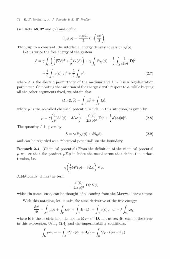
74 R. H. Nochetto, A. J. Salgado & S. W. Walker
(see Refs. 58, 32 and 62) and define
Θfs(φ) =cos θs
2sin(πφ
2
).
Then, up to a constant, the interfacial energy density equals γΘfs(φ).Let us write the free energy of the system
E = γ
∫Ω
(δ
2|∇φ|2 +
1δW(φ)
)+ γ
∫Γ
Θfs(φ) +12
∫Ω
1ε(φ)
|D|2
+12
∫Ω
ρ(φ)|u|2 +λ
2
∫Ω
q2, (2.7)
where ε is the electric permittivity of the medium and λ > 0 is a regularizationparameter. Computing the variation of the energy E with respect to φ, while keepingall the other arguments fixed, we obtain that
〈DφE, φ〉 =∫
Ω
µφ+∫
Γ
Lφ,
where µ is the so-called chemical potential which, in this situation, is given by
µ = γ
(1δW ′(φ) − δ∆φ
)− ε′(φ)
2ε(φ)2|D|2 +
12ρ′(φ)|u|2. (2.8)
The quantity L is given by
L = γ(Θ′fs(φ) + δ∂nφ), (2.9)
and can be regarded as a “chemical potential” on the boundary.
Remark 2.4. (Chemical potential) From the definition of the chemical potentialµ we see that the product µ∇φ includes the usual terms that define the surfacetension, i.e.
γ
(1δW ′(φ) − δ∆φ
)∇φ.
Additionally, it has the term
− ε′(φ)2ε(φ)2
|D|2∇φ,
which, in some sense, can be thought of as coming from the Maxwell stress tensor.
With this notation, let us take the time derivative of the free energy:
dE
dt=∫
Ω
µφt +∫
Γ
Lφt +∫
Ω
E ·Dt +∫
Ω
ρ(φ)u · ut + λ
∫Ω
qqt,
where E is the electric field, defined as E := ε−1D. Let us rewrite each of the termsin this expression. Using (2.4) and the impermeability conditions,∫
Ω
µφt = −∫
Ω
µ∇ · (φu + Jφ) =∫
Ω
∇µ · (φu + Jφ).
October 23, 2013 15:48 WSPC/103-M3AS 1350047
Electrowetting 75
Using (2.5) ∫Ω
E ·Dt = −∫
Ω
E · (qu + JD).
For the boundary term, we introduce the material derivative at the boundaryφ = φt + uτ∂τφ and rewrite∫
Γ
Lφt =∫
Γ
L(φ− uτ∂τφ).
Notice that σ(σu)t = ρut + 12ρtu, so that using (2.2), and integrating by parts, we
obtain∫Ω
ρ(φ)u · ut =∫
Ω
F · u − 12
∫Ω
ρ(φ)t|u|2 +∫
Γ
η(S(u) · n) · uτ −∫
Ω
η|S(u)|2.
Finally, using (2.6) and the impermeability condition (qu + JD) · n|Γ = 0,
λ
∫Ω
qqt = −λ∫
Ω
q∇ · (qu + JD) = λ
∫Ω
∇q · (qu + JD).
With the help of these calculations, we find that the time-derivative of the freeenergy can be rewritten as
E = −∫
Ω
µ∇φ · u +∫
Ω
Jφ · ∇µ+∫
Γ
L(φ− uτ∂τφ) −∫
Ω
E · (qu + JD)
+∫
Ω
F · u − 12
∫Ω
ρ′(φ)φt|u|2 +∫
Γ
η(S(u) · n) · uτ −∫
Ω
η|S(u)|2
+λ
2
∫Ω
u · ∇(q2) + λ
∫Ω
∇q · JD. (2.10)
From (2.10), we can identify the power of the system, i.e. the time derivativeof the work W of internal forces, upon collecting all terms having a scalar productwith the velocity u,
W =∫
Ω
F · u −∫
Ω
µ∇φ · u −∫
Ω
qE · u +λ
2∇(q2) · u − 1
2
∫Ω
ρ′(φ)φtu · u.
We assume that the system is closed, i.e. there are no external forces. This impliesthat W ≡ 0 and we obtain an expression for the forces F acting on the fluid,
F = µ∇φ+ qE +12ρ′(φ)φtu −∇
(λ
2q2).
Using the first law of thermodynamics
dE
dt=
dW
dt− T dS
dt,
October 23, 2013 15:48 WSPC/103-M3AS 1350047
76 R. H. Nochetto, A. J. Salgado & S. W. Walker
where the absolute temperature is denoted by T and the entropy by S, we canconclude that
T S =∫
Ω
η|S(u)|2 −∫
Ω
E · JD +∫
Ω
Jφ · ∇µ+ λ
∫Ω
∇q · JD
+∫
Γ
η(S(u) · n) · uτ +∫
Γ
L(φ− uτ∂τφ).
To find an expression for the fluxes we introduce, in the spirit of Onsager,53,58 adissipation function Φ. Since this must be a positive-definite function on the fluxes,the simplest possible expression for a dissipation function is quadratic and diagonalin the fluxes, e.g.
Φ =12
∫Ω
1M
|Jφ|2 +α
2
∫Γ
φ2 +12
∫Ω
1K
|JD|2 +12
∫Γ
β|uτ |2,
where all the proportionality constants, in principle, can depend on the phase φ.Here, M is known as the mobility, K the conductivity and β the slip coefficient.Using Onsager’s relation
Remark 2.5. (Constitutive relations) Definitions (2.11) can also be obtained bysimply saying that the constitutive relations of the fluxes depend linearly on thegradients, which is implicitly postulated in the form of the dissipation function Φ.
Since, in practical settings, there is an externally applied voltage (which is goingto act as the control mechanism) we introduce a potential V and then the electricfield is given by E = −∇V with V = V0 on ∂Ω, where V0 is the voltage applied.
To summarize, we obtain the following system of equations for the phase variableφ and the chemical potential µ,
In addition, we have the equation for the electric charges q,qt + ∇ · (qu) = ∇ · [K(φ)∇(λq + V )], in Ω,
K(φ)∇(λq + V ) · n = 0, on Γ,(2.14)
and voltage V , −∇ · (ε(φ)∇V ) = qχΩ, in Ω,
V = V0, on ∂Ω,
∂nV = 0, on ∂Ω ∩ Γ,
(2.15)
where
ε(φ) = ε(φ)χΩ + εDχΩ\Ω,
with εD being the value of the permittivity on the dielectric plates Ω\Ω, so εD isconstant there.
Remark 2.6. (Generalized Navier boundary condition) In (2.13), the boundarycondition for the tangential velocity is known as the generalized Navier boundarycondition (GNBC), and it is aimed at resolving the so-called contact line paradoxof the movement of a two-phase fluid on a solid wall. The reader is referred to,for instance, Refs. 57, 58 and 32 for a discussion of its derivation. Another remedyfor the paradox is discussed in Ref. 41 by considering Navier–Stokes coupled to aCahn–Hilliard–van der Waals phase-field model. Through an analytic solution andasymptotic analysis, they show that their model allows for a moving contact lineeven with no-slip conditions for the velocity.
Another type of GNBC has been developed in Refs. 70 and 71 which proposesan “interface formation” model (Shikhmurzaev model). Extra equations are intro-duced to model variable surface tension (with an equation of state) and is cou-pled to a slip boundary condition (see Ref. 50 for numerical simulations of thismodel in a microscopic region near the contact line). An asymptotic analysis of the
October 23, 2013 15:48 WSPC/103-M3AS 1350047
78 R. H. Nochetto, A. J. Salgado & S. W. Walker
Shikhmurzaev model is given in Refs. 13 and 14, but raises an issue of a “missingboundary condition.”
Despite the large controversy and discussion around the validity of this boundarycondition, see for instance Refs. 19 and 71, we shall take the GNBC as given andwill not discuss its applicability and/or consequences here.
Remark 2.7. (Galilean invariance) As discussed in Refs. 3 and 1 (Remark 2.2),the term 1
2ρ′(φ)|u|2 is not an objective scalar, which makes our model not frame
invariant. This basically amounts to choosing a frame of reference and, consequently,should not be seen as a serious limitation of our approach. In contrast, it is notcompletely clear how to carry out an analysis of, for instance, the frame indifferentmodel presented in Ref. 1.
2.2. Nondimensionalization
Here we present appropriate scalings so that we may write Eqs. (2.12)–(2.15) in non-dimensional form. Table 1 shows some typical values for the material parametersappearing in the model (see also Ref. 46). Consider the following scalings:
u = u/Us (choose Us), x = x/Ls (choose Ls), t = t/ts,
ts = Ls/Us, µ = µ/µs, µs = γ/Ls,
q = q/qs, qs = Vs/λ, V = V/Vs, (choose Vs),
ε = ε/εs, δ = δ/Ls, M = M/Ms,
K = K/Ks, Ca =ηsUs
γ, Re =
ρsUsLs
ηs,
We =ρsU
2s Ls
γ, Bo =
εsV2s
Lsγ, IE =
ρsU2s
qsVs,
SP =γ
α/ts, MO =
γMs
L2sUs
, KO =VsKs
LsqsUs,
CH =qsL
2s
Vsεs,
where Ca is the capillary number, Re is the Reynolds number, We is the Webernumber, Bo is the electrowetting Bond number, IE is the ratio of fluid forces toelectrical forces, SP is the ratio of surface tension to “phase field forces,” MO is a(non-dimensional) mobility coefficient, KO is a conductivity coefficient, and CH isan electric charge coefficient.
Let us now make the change of variables. To simplify notation, we drop thetildes, and consider all variables and differential operators as non-dimensional. Thefluid equations read:
D(ρu)Dt
− 1Re
∇ · (ηS(u)) + ∇p =1
Weµ∇φ− 1
IEq∇(V + q) +
12ρ′(φ)φtu, in Ω,
∇ · u = 0, in Ω,
u · n = 0, on Γ,
βuτ + ηS(u)nτ =1
Ca(Θ′
fs(φ) + δ∂nφ)∂τφ, on Γ.
The phase-field equations change to (again dropping the tilde)φt + u · ∇φ = MO∇ · (M(φ)∇µ), in Ω,
Performing the change of variables on the charge transport equation givesqt + ∇ · (qu) = KO∇ · (K(φ)∇(q + V )), in Ω,
n · ∇(q + V ) = 0, on Γ.
October 23, 2013 15:48 WSPC/103-M3AS 1350047
80 R. H. Nochetto, A. J. Salgado & S. W. Walker
Lastly, for the electrostatic equation we obtain−∇ · (ε(φ)∇V ) = CHqχΩ, in Ω,
V = V0/Vs, on ∂Ω,
∂nV = 0, on ∂Ω ∩ Γ,
where ε(φ) has been normalized by εs.To alleviate the notation, for the rest of our discussion we will set all the nondi-
mensional groups (Ca,Re,We,Bo, IE, SP,MO,KO and CH) to one. If needed, thedependence of the constants on all these parameters can be traced by following ourarguments. Moreover, we must note that if a simplification of this model is desired,then these scalings must serve as a guide to decide which effects are dominant.
2.3. Tangential derivatives at the boundary
As we can see from (2.12) and (2.13), our model incorporates tangential derivativesof the phase variable φ at the boundary Γ. Unfortunately, in the analysis, we are notcapable of dealing with these terms. Therefore, we propose some simplifications.
The first possible simplification is simply to ignore the terms that contain thistangential derivative; see Ref. 27. However, it is our feeling that the presence ofthem is important, specially in dealing with the contact angle in the GNBC.
A second possibility would be to add an ad hoc term of the form ∆Γφ on theboundary condition for the phase variable, where by ∆Γ we denote the Laplace–Beltrami operator on Γ. A similar approach has been followed, in a somewhatdifferent context, for instance, by Pruss et al.56 and Cherfils et al.21 However, thiscondition might lead to lack of conservation of φ, which is an important feature ofphase field models based on the Cahn–Hilliard equation.
Finally, the approach that we propose is to recall that, in principle, the phasefield variable must be constant in the bulk of each of the phases and so ∂τφ ≈ 0there. Moreover, in the sharp interface limit this tangential derivative must be aDirac measure supported on the interface. Therefore we define a function
ψ(φ) =1Ls
1δe−
φ22δ , where δ is non-dimensional, (2.16)
and replace all the instances of ∂τφ by ψ(φ). We are aware that this is a majorassumption in our model. However, as we mentioned above, it is not possible tocarry out any analysis if we leave such terms without modification. It is of nosurprise then that, to the best of our knowledge, there is no existence results forsystems with an unmodified GNBC.
2.4. Contact line pinning
Simply put, the contact line pinning (hysteresis) is a frictional effect that occursat the three-phase contact line, and is rather controversial. We refer the reader toRefs. 74 and 73 for an explanation about its origins and possible dependencies. Let
October 23, 2013 15:48 WSPC/103-M3AS 1350047
Electrowetting 81
us here only mention that, macroscopically, the pinning force has a threshold valueand, thus, it should depend on the stress at the contact line. It is important to takeinto account contact line pinning since, as observed in Refs. 74 and 73, it is crucialfor capturing the true time scales of the problem.
We propose a phenomenological approach to deal with this effect. From theGNBC,
βuτ + ηS(u)nτ = γ(Θ′fs(φ) + δ∂nφ)ψ(φ),
we can see that, to recover no-slip conditions, one must set the slip coefficient βsufficiently large. On the contrary, when β is small, one obtains an approximation offull slip conditions. A simple dimensional argument then shows that β = η, where has the dimensions of inverse length. Therefore, we propose the slip coefficient tohave the following form
β = η(φ)(φ,S), (2.17)
with
(φ,S) =C
Ls
1δ, |φ| > 1
2,
1δ, |φ| ≤ 1
2, and |S(u)nτ | Tp,
1, |φ| ≤ 12, and |S(u)nτ | ≈ Tp,
where C is a (phenomenological) constant and δ is the non-dimensional transitionlength. For the purposes of analysis, we face the same difficulties in this expression asin Sec. 2.3. Therefore, we will use this to model pinning in the numerical examples,but leave it out of the analysis.
Let us illustrate the effect of introducing such a term by means of a numericalexample. We implemented the method of Ref. 62 and a variation of it for the slipcoefficient β defined as in (2.17). We consider the evolution of a bubble on aninclined plane under the action of gravity. The material parameters are ρ1/ρ2 =50, η1/η2 = 10,M1 = M2 = 10−2, α = 10−3, γ = 10 and θs = 90. For the casewithout pinning we set β1 = β2 = 1.5 and C = 1.5 for the pinning case. The timestep is set to ∆t = 5× 10⁻⁴. The mesh is adaptively refined near the interface andit is such that the local mesh size away from the interface is about 10−2 and nearit 8× 10⁻³. The interface thickness is δ = 10−2. Figure 2 shows the evolution every0.002 time units until t = 2.2× 10⁻². Notice that, although there is movement, thedynamics are indeed slowed down when compared to the case of no pinning. This,evidently, needs further investigation which we defer to a future work.
Remark 2.8. (Contact line pinning penalization) We essentially model pinning bya penalty approach. Thus, it does not exactly capture the pinning phenomena, i.e.a droplet getting stuck in a configuration with contact angles different from theequilibrium angles determined by the classic Young’s equation. Instead, it only acts
October 23, 2013 15:48 WSPC/103-M3AS 1350047
82 R. H. Nochetto, A. J. Salgado & S. W. Walker
Fig. 2. (Color online) Evolution of a droplet under the action of gravity with and without pinning.Colors represent the droplet with pinning as in (2.17) whereas the black solid line shows theposition of the interface without pinning. The material parameters are ρ1/ρ2 = 50, η1/η2 =10, M1 = M2 = 10−2, α = 10−3, γ = 10, θs = 90, β1 = β2 = C = 1.5. The interface thicknessis δ = 10−2. The configuration is shown for times t = 0 and then every 0.002 time units untilt = 2.2 × 10⁻².
as an additional retarding force to the contact line motion. However, the GNBCdoes allow for contact angle hysteresis when the droplet is in motion as was shownby a formal argument in Ref. 58 when using the GNBC.
3. Formal Weak Formulation and Formal Energy Estimate
In this section we obtain a weak formulation for problem (2.12)–(2.15) and show aformal energy estimate, which serves as an a priori estimate and the basic relationon which our existence theory is based. We mention that Ref. 15 considers a coupledCahn–Hilliard and Navier–Stokes model with different densities (see Ref. 16 forsimulations of their model and comparisons with experiments). However, they couldonly show local existence of a very unique regular solution; existence of weakersolutions was left open in Ref. 15.
The derivation of our formal weak formulation is on the basis of energy argu-ments. The main novelty in our approach is that we do not need to assume that thedensity is constant nor that the density contrast is small. This is possible thanks tothe way we have written the convective term in (2.2a), since this allows us to useidentity (2.3). See Remark 2.2 for more details.
3.1. Formal weak formulation
To obtain a weak formulation of the problem, we begin by multiplying the firstequation of (2.12) by φ, the second by µ and integrating in Ω. After integration byparts, taking into account the boundary conditions, we arrive at
〈φt, φ〉 + 〈u · ∇φ, φ〉 + 〈M(φ)∇µ,∇φ〉 = 0 (3.1a)
October 23, 2013 15:48 WSPC/103-M3AS 1350047
Electrowetting 83
and
〈µ, µ〉 =γ
δ〈W ′(φ), µ〉 + γδ〈∇φ,∇µ〉 − 1
2〈ε′(φ)|∇V |2, µ〉 +
12〈ρ′(φ)|u|2, µ〉
+α[φt + uτψ(φ), µ] + γ[Θ′fs(φ), µ]. (3.1b)
Multiply the first equation of (2.13) by w such that w · n|Γ = 0, the second by pand integrate in Ω. Integration by parts on the first equation, in conjunction withthe boundary conditions and (2.16), yields
Let W be a function that equals zero on ∂Ω. Multiply the equation for the electricpotential (2.15) by W , integrate in Ω to obtain
〈ε(φ)∇V,∇W 〉Ω = 〈q,W 〉. (3.4)
Given the way the model has been derived, it is clear that an energy estimatemust exist. Before we obtain it, let us show a comparison result a la Gronwall.
Lemma 3.1. (Gronwall) Let f, g, h, w : [0, T ] → R be measurable and positivefunctions such that
f(t)2 +∫ t
0
g(s)ds ≤ h(t) +∫ t
0
f(s)w(s)ds, ∀ t ∈ [0, T ]. (3.5)
October 23, 2013 15:48 WSPC/103-M3AS 1350047
84 R. H. Nochetto, A. J. Salgado & S. W. Walker
Then
sups∈[0,T ]
f(s)2 +12
∫ T
0
g(s)ds ≤ 4 sups∈[0,T ]
h(s) + 4T∫ T
0
w2(s)ds, ∀ t ∈ [0, T ].
Proof. Take, in (3.5), t = t0, where
t0 = argmaxf(s) : s ∈ [0, T ],
then
f(t0)2 +∫ t0
0
g(s)ds ≤ maxs∈[0,T ]
h(s) + f(t0)∫ t0
0
w(s)ds
≤ maxs∈[0,T ]
h(s) +12f(t0)2 +
(∫ T
0
w(s)ds
)2
.
Canceling the common factors, applying the Cauchy–Schwarz inequality on theright and taking the supremum on the left-hand side we obtain the result.
Remark 3.1. (Exponential in time estimates) The main advantage of usingLemma 3.1 to obtain a priori estimates, as opposed to a standard argument invok-ing Gronwall’s inequality, is that we can avoid exponential dependence on the finaltime T .
The following result provides the formal energy estimate.
Theorem 3.1. (Stability) If there is a solution to (2.12)–(2.15), then it must sat-isfy the following estimate:
sups∈(0,T ]
∫Ω
[12ρ(φ)|u|2 +
λ
4q2 + γ
(δ
2|∇φ|2 +
1δW(φ)
)]+∫
Ω
14ε(φ)|∇V |2
+ γ
∫Γ
Θfs(φ)
+∫ T
0
∫Ω
[η(φ)|S(u)|2 +M(φ)|∇µ|2
+K(φ)|∇(λq + V )|2] +∫
Γ
[β(φ)|uτ |2 + α|φt + uτψ(φ)|2]
≤∫
Ω
[12ρ(φ)|u|2 + q2 + γ
(δ
2|∇φ|2 +
1δW(φ)
)+
12|V0|2
]+∫
Ω
(ε(φ)|∇V |2 + εM |∇V0|2
)+ γ
∫Γ
Θfs(φ) ∣∣∣∣
t=0
+ sups∈[0,T ]
∫Ω
εM |∇V0|2 +∫
Ω
1λ|V0|2(t)
+ cT∫ T
0
[∫Ω
εM |∇V0,t|2 +4λ
∫Ω
|V0,t|2], (3.6)
where c does not depend on T .
October 23, 2013 15:48 WSPC/103-M3AS 1350047
Electrowetting 85
Proof. We first deal with the Navier–Stokes and Cahn–Hilliard equations in a wayvery similar to Theorem 3.1 of Ref. 62. Set w = u in (3.2a) and notice that⟨
Integrate in time over [0, t], with 0 < t < T and integrate by parts the right-handside. Repeated applications of the Cauchy–Schwarz inequality give us∫
Ω
[12ρ(φ)|u|2 +
λ
4q2 + γ
(δ
2|∇φ|2 +
1δW(φ)
)]+∫
Ω
14ε(φ)|∇V |2
+ γ
∫Γ
Θfs(φ) ∣∣∣∣
t
+∫ t
0
∫Ω
[η(φ)|S(u)|2 +M(φ)|∇µ|2
+K(φ)|∇(λq + V )|2] +∫ t
0
∫Γ
[β(φ)|uτ |2 + α|φt + uτψ(φ)|2]
≤∫
Ω
[12ρ(φ)|u|2 + q2 + γ
(δ
2|∇φ|2 +
1δW(φ)
)]+∫
Ω
ε(φ)|∇V |2
+ γ
∫Γ
Θfs(φ) ∣∣∣∣
t=0
+∫
Ω
εM (|∇V0|2(t) + |∇V0|2(0))
+∫
Ω
[1λ|V0|2(t) +
12|V0|2(0)
]+ c
∫ t
0
∫Ω
εM |∇V0,t|2 +4λ
∫Ω
|V0,t|21/2
×[λ
4
∫Ω
q2 +∫
Ω
14ε(φ)|∇V |2
]1/2
,
where εM is the maximal value of the function ε(φ).Finally, if we set
f(t) =∫
Ω
[12ρ(φ)|u|2 +
λ
4q2 + γ
(δ
2|∇φ|2 +
1δW(φ)
)]+∫
Ω
14ε(φ)|∇V |2 + γ
∫Γ
Θfs(φ)
(t),
g(t) =∫
Ω
[η(φ)|S(u)|2 +M(φ)|∇µ|2 +K(φ)|∇(λq + V )|2]
+∫
Γ
[β(φ)|uτ |2 + α|φt + uτψ(φ)|2]
(t),
October 23, 2013 15:48 WSPC/103-M3AS 1350047
Electrowetting 87
h(t) =∫
Ω
[12ρ(φ)|u|2 + q2 + γ
(δ
2|∇φ|2 +
1δW(φ)
)]+∫
Ω
ε(φ)|∇V |2 + γ
∫Γ
Θfs(φ) ∣∣∣∣
0
+∫
Ω
εM (|∇V0|2(t) + |∇V0|2(0)) +∫
Ω
[1λ|V0|2(t) +
12|V0|2(0)
],
w(t) =∫
Ω
εM |∇V0,t|2 +4λ
∫Ω
|V0,t|21/2
,
then an application of Lemma 3.1 gives the desired estimate.
4. The Fully Discrete Problem and Its Analysis
In this section we introduce a spacetime discrete problem that is used to approxi-mate the electrowetting problem (3.1)–(3.4). Using this discrete problem, and theresult of Theorem 3.1, we will prove that a time-discrete version of our problemalways has a solution. Moreover, in Sec. 5, we will base our numerical experimentson a variant of the problem defined here.
The fully discrete problem that we present below uses a backward Euler tech-nique to handle time discretization and finite-element-like techniques for space. Inthis respect our approach differs from, for instance Refs. 27, 15 and 30, where thereis no time discretization and the space discretization is usually handled via a spe-cial basis consisting of eigenfunctions of the underlying (linearized) operators. Ourapproach, although makes the analysis more complicated, is motivated by the factthat, in principle, it is possible to implement our fully discrete problem. There-fore, the results of this section provide convergence of a fully practical numericalscheme.
The particular structure of the fully discrete problem is such that, again usingenergy arguments, an analogue of Theorem 3.1 can be obtained. Being that weare now in finite dimension, this a priori estimate guarantees, via a fixed pointargument, the existence of solutions.
4.1. Definition of the fully discrete problem
To discretize in time, as discussed in Sec. 1.1, we divide the time interval [0, T ]into subintervals of length ∆t > 0. Recall that the time increment operator d wasintroduced in (1.4) and the time average operator (·) in (1.5).
To discretize in space, we introduce a parameter h > 0 and let Wh ⊂H1
(Ω),Qh ⊂ H1(Ω),Xh ⊂ V and Mh ⊂ L2R=0(Ω) be finite dimensional subspaces.
We require the following compatibility condition between the spaces Wh and Qh:
Wh|Ω ∈ Qh, ∀Wh ∈ Wh. (4.1)
October 23, 2013 15:48 WSPC/103-M3AS 1350047
88 R. H. Nochetto, A. J. Salgado & S. W. Walker
Moreover, we require that the pair of spaces (Xh,Mh) satisfies the so-called LBBcondition (see Refs. 33, 18 and 28), that is, there exists a constant c independentof h such that
c‖ph‖L2 ≤ supvh∈Xh
∫Ωph∇ · vh
‖vh‖H1, ∀ ph ∈ Mh. (4.2)
Finally, we assume that if Y is any of the continuous spaces and Yh the correspond-ing subspace, then h1 < h2 implies Yh2 ⊂ Yh1 . Moreover, the family of spacesYhh>0, is “dense in the limit.” In other words, for every h > 0 there is a contin-uous operator Ih : Y → Yh such that when h→ 0
‖y − Ihy‖Y → 0, ∀ y ∈ Y.
The space Wh will be used to approximate the voltage; Qh the charge, phasefield and chemical potential; and Xh,Mh the velocity and pressure, respectively.Finally, to account for the boundary conditions on the voltage, we denote
Wh(V k+10 ) = Wh + V k+1
0 .
Remark 4.1. (Finite elements) The introduced spaces can be easily constructedusing, for instance, finite elements, see Refs. 33, 18, 28 and 25 for details. Thecompatibility condition (4.1) can be easily attained. For instance, one can requirethat the mesh is constructed in such a way that for all cells K in the triangulation Th,
K ∩ Ω = ∅ ⇔ K ∩ (Ω\Ω) = ∅,
and the polynomial degree of the space Qh is no less than that of Wh. Finally, weremark that the nestedness assumption is done merely for convenience.
h be suitable approximations of the initialcharge, phase field and velocity, respectively.
Time Marching: For 0 ≤ n ≤ N − 1 we compute
(V n+1h , qn+1
h , φn+1h , µn+1
h ,un+1h , pn+1
h ) ∈ Wh(V n+10 ) × Q3
h × Xh × Mh,
that solve:
〈ε(φn+1h )∇V n+1
h ,∇Wh〉Ω = 〈qn+1h ,Wh〉, ∀Wh ∈ Wh, (4.3)⟨
dqn+1h
∆t, rh
⟩− 〈qn
hun+1h ,∇rh〉
+ 〈K(φnh)∇(λqn+1
h + V n+1h ),∇rh〉 = 0, ∀ rh ∈ Qh, (4.4)
October 23, 2013 15:48 WSPC/103-M3AS 1350047
Electrowetting 89
⟨dφn+1
h
∆t, φh
⟩+ 〈un+1
h · ∇φnh , φh〉
+ 〈M(φnh)∇µn+1
h ,∇φh〉 = 0, ∀ φh ∈ Qh (4.5)
〈µn+1h , µh〉 =
γ
δ〈W ′(φn
h) + Adφn+1h , µh〉 + γδ〈∇φn+1
h ,∇µh〉
− 12〈E(φn+1
h , φnh)|∇V n+1
h |2, µh〉 +12〈ρ′(φn
h)unh · un+1
h , µh〉
+α
[dφn+1
h
∆t+ un+1
hτ ψ(φnh), µh
]+ γ[Θ′
fs(φnh) + Bdφn+1
h , µh]
∀ µh ∈ Qh, (4.6)
where we introduced
E(ϕ1, ϕ2) =∫ 1
0
ε′(sϕ1 + (1 − s)ϕ2)ds, (4.7)
⟨ρ(φn+1
h )un+1h − ρ(φn
h)unh
∆t,wh
⟩+ 〈ρ(φn
h)unh · ∇un+1
h ,wh〉
+12〈∇ · (ρ(φn
h)unh)un+1
h ,wh〉 + 〈η(φnh)S(un+1
h ),S(wh)〉 − 〈pn+1h ,∇ ·wh〉
+ [β(φnh)un+1
hτ ,whτ ] + α[un+1hτ ψ(φn
h),whτψ(φnh)]
= 〈µn+1h ∇φn
h ,wh〉 − 〈qnh∇(λqn+1
h + V n+1h ),wh〉
+12
⟨ρ′(φn
h)dφn+1
h
∆tun
h ,wh
⟩− α
[dφn+1
h
∆t,whτψ(φn
h)]
∀wh ∈ Xh, (4.8a)
〈ph,∇ · un+1h 〉 = 0, ∀ ph ∈ Mh. (4.8b)
Remark 4.2. (Stabilization parameters) Notice that, in (4.6), we have introducedtwo stabilization parameters, namely A and B. Their purpose is twofold. First,they will allow us to treat the nonlinear terms explicitly while still being able tomaintain stability of the scheme, see Proposition 4.1 below. Second, when studyingconvergence of this problem, the presence of these terms will allow us to obtainfurther a priori estimates on discrete solutions which, in turn, will help in passing tothe limit, see Theorem 6.1. We must mention that, this way of writing nonlinearitiesis related to the splitting of the energy into a convex and concave part proposed inRef. 75. See also Refs. 68 and 67.
Remark 4.3. (Derivative of the permittivity) Notice that (4.7), i.e. the definitionof the term E , is a highly nonlinear function of its arguments (unless ε is of avery specific type). As the reader has seen in the derivation of the energy law(Theorem 3.1), the treatment of the term involving the derivative of the permittivity
October 23, 2013 15:48 WSPC/103-M3AS 1350047
90 R. H. Nochetto, A. J. Salgado & S. W. Walker
is subtle. In the fully discrete setting this is additionally complicated by the factthat we need to deal with quantities at different time layers. The reason to writethe derivative of the permittivity in this form is that
E(ϕ1, ϕ2) =
ε(ϕ1) − ε(ϕ2)ϕ1 − ϕ2
, ϕ1 = ϕ2,
ε′(ϕ1), ϕ1 = ϕ2,
which will allow us to obtain the desired cancellations.
The following subsections will be devoted to the analysis of problem (4.3)–(4.8).For convenience, we define
φnh :=
dφnh
∆t+ un
hτψ(φn−1h ).
4.2. A priori estimates and existence
Let us show that, if problem (4.3)–(4.8) has a solution, it satisfies a discrete energyinequality similar to the one stated in Theorem 3.1. To do this, we first require thefollowing formula, whose proof is straightforward.
Lemma 4.1. (Summation by parts) Let fnm−1n=0 and gnm−1
n=0 be sequences andassume f−1 = g−1 = 0. Then we have
m−1∑n=0
(dgn)fn = fm−1gm−1 −m−2∑n=0
gn(dfn+1). (4.9)
Proposition 4.1. (Discrete stability) Assume that the stabilization parameters Aand B are chosen so that
A ≥ 12
supξ∈R
W ′′(ξ), B ≥ 12
supξ∈R
Θ′′fs(ξ). (4.10)
The solution to (4.3)–(4.8), if it exists, satisfies the following a priori estimate
h ≡ 0 for convenience in writing (4.11). The constantc depends on the constants γ, δ, α, the data of the problem u0
h, φ0h, q
0h, V0,∆t and T,
but it does not depend on the discretization parameters h or ∆t, nor the solution ofthe problem.
October 23, 2013 15:48 WSPC/103-M3AS 1350047
Electrowetting 91
Proof. We repeat the steps used to prove Theorem 3.1, i.e. set wh = 2∆tun+1h in
(4.8a), ph = pn+1h in (4.8b), φh = 2∆tµn+1
h in (4.5), µh = −2dφn+1h in (4.6) and
rh = 2∆t(λqn+1h +V n+1
h ) in (4.4). To treat the time-derivative terms in the discretemomentum equation, we use the identity
2un+1h · (ρ(φn+1
h )un+1h − ρ(φn
h)unh)
= ρ(φn+1h )|un+1
h |2 − ρ(φnh)|un
h |2 + ρ(φnh)|dun+1
h |2;
see Refs. 38 and 39. To obtain control on the explicit terms involving the derivativesof the Ginzburg–Landau potential W and the surface energy density Θfs , noticethat, for instance,
W(φn+1h ) −W(φn
h) = W ′(φnh)dφn+1
h +12W ′′(ξ)(dφn+1
h )2,
for some ξ. Choosing the stabilization constant according to (4.10) (cf. Refs. 68, 67,69 and 62), we deduce that∫
Ω
(W ′(φnh) + Adφn+1
h )dφn+1h ≥
∫Ω
dW(φn+1h ).
Adding (4.4)–(4.8) yields,
d‖σ(φn+1h )un+1
h ‖2L2 + ‖σ(φn
h)dun+1h ‖2
L2 + λ(d‖qn+1h ‖2
L2 + ‖dqn+1h ‖2
L2)
+ γδ(d‖∇φn+1h ‖2
L2 + ‖∇dφn+1h ‖2
L2) +2γδ
∫Ω
dW(φn+1h )
+ 2γ∫
Γ
dΘfs(φn+1h ) + 2∆t
[∥∥∥√η(φnh)S(un+1
h )∥∥∥2
L2
+∥∥∥√β(φn
h)un+1hτ
∥∥∥2
L2(Γ)+∥∥∥√M(φn
h)∇µn+1h
∥∥∥2
L2
+∥∥∥√K(φn
h)∇(λqn+1h + V n+1
h )∥∥∥2
L2+ α
∥∥∥∥dφn+1h
∆t+ un+1
hτ ψ(φnh)∥∥∥∥2
L2(Γ)
]+ 2〈dqn+1
h , V n+1h 〉 ≤ 〈E(φn+1
h , φnh)|∇V n+1
h |2, dφn+1h 〉. (4.12)
Take the difference of (4.3) at time-indices n+ 1 and n to obtain
〈d(ε(φn+1h )∇V n+1
h ),∇Wh〉Ω = 〈dqn+1h ,Wh〉,
and set Wh = 2(V n+1h − V n+1
0 ). In view of (1.6) we have
2d(ε(φn+1h )∇V n+1
h ) · ∇V n+1h
= d(ε(φn+1h )|∇V n+1
h |2) + ε(φnh)|∇dV n+1
h |2 + d(ε(φn+1h ))|∇V n+1
h |2,
October 23, 2013 15:48 WSPC/103-M3AS 1350047
92 R. H. Nochetto, A. J. Salgado & S. W. Walker
whence
d∥∥∥√ε(φn+1
h )∇V n+1h
∥∥∥2
L2(Ω)+∥∥∥√ε(φn
h)∇dV n+1h
∥∥∥2
L2(Ω)
+∫
Ω
dε(φn+1h )|∇V n+1
h |2
= 2〈dqn+1h , V n+1
h 〉 − 2〈dqn+1h , V n+1
0 〉
+ 2〈d(ε(φn+1h )∇V n+1
h ),∇V n+10 〉Ω . (4.13)
Add (4.12) and (4.13). Notice that, since the permittivity is assumed constanton Ω\Ω, on the left-hand side of the resulting inequality we have the followingterm: ∫
Ω
(dε(φn+1h ) − E(φn+1
h , φnh)dφn+1
h )|∇V n+1h |2 = 0,
where we used the definition of E , see (4.7) and Remark 4.3. Therefore, we obtain
d‖σ(φn+1h )un+1
h ‖2L2 + ‖σ(φn
h)dun+1h ‖2
L2 + λ
(d‖qn+1
h ‖2L2 +
12‖dqn+1
h ‖2L2
)+ γδ(d‖∇φn+1
h ‖2L2 + ‖∇dφn+1
h ‖2L2) +
2γδ
∫Ω
dW(φn+1h )
+ d∥∥∥√ε(φn+1
h )∇V n+1h
∥∥∥2
L2(Ω)+∥∥∥√ε(φn
h)∇dV n+1h
∥∥∥2
L2(Ω)
+ 2γ∫
Γ
dΘfs(φn+1h ) + 2∆t
[∥∥∥√η(φnh)S(un+1
h )∥∥∥2
L2
+∥∥∥√β(φn
h)un+1hτ
∥∥∥2
L2(Γ)+∥∥∥√M(φn
h)∇µn+1h
∥∥∥2
L2
+∥∥∥√K(φn
h)∇(λqn+1h + V n+1
h )∥∥∥2
L2+ α
∥∥∥∥dφn+1h
∆t+ un+1
hτ ψ(φnh)∥∥∥∥2
L2(Γ)
]≤ −2〈dqn+1
h , V n+10 〉 + 2〈d(ε(φn+1
h )∇V n+1h ),∇V n+1
0 〉Ω . (4.14)
Summing (4.14) for n = 0, . . . ,m − 1, using summation by parts (4.9) (setµ0
h ≡ 0, V 0h ≡ 0), applying the Cauchy–Schwarz and weighted Young’s inequality,
we obtain the result.
Remark 4.4. (Compatibility) Notice that condition (4.1) is needed to obtain thestability estimate, otherwise 2∆t(λqn+1
h + V n+1h ) would not be an admissible test
function for (4.4).
The a priori estimate (4.11) allows us to conclude that, for all h > 0 and ∆t > 0,problem (4.3)–(4.8) has a solution.
October 23, 2013 15:48 WSPC/103-M3AS 1350047
Electrowetting 93
Theorem 4.1. (Existence) Assume that the discrete spaces satisfy assumptions(4.1) and (4.2), the stabilization parameters A,B are chosen as in Proposition 4.1.Then, for all h > 0 and ∆t > 0, problem (4.3)–(4.8) has a solution. Moreover, anysolution satisfies estimate (4.11).
Proof. The idea of the proof is to use the “method of a priori estimates” at eachtime step. In other words, for each time step we define a map Ln+1 in such a waythat a fixed point of Ln+1, if it exists, is a solution of our problem. Then, with theaid of the previously shown a priori estimates we show that Ln+1 does indeed havea fixed point.
We proceed by induction in the discrete time and assume that we have shownthat the problem has a solution up to n. For each n = 0, . . . , N − 1, we define
Notice that a fixed point of Ln+1 is precisely a solution of the discrete prob-lem (4.3)–(4.8).
To show the existence of a fixed point we must prove that:
• The operator Ln+1 is well defined.• If there is a X = (Vh, qh, φh, µh,uh, ph) for which X = ωLn+1X , for some ω ∈
[0, 1], then
‖X‖ ≤M, (4.21)
where M > 0 does not depend on X or ω.
Then, an application of the Leray–Schauder theorem29,76 will allow us to conclude.Moreover, since a fixed point of Ln+1 is precisely a solution of our problem, Propo-sition 4.1 gives us the desired stability estimate for this solution.
Let us then proceed to show these two points:
The operator Ln+1 is well defined : Clearly, for any given φh, and qh, the system(4.15)–(4.16) is positive definite and, thus, there are unique Vh and qh. Havingcomputed Vh and qh we then notice that (4.19) and (4.20) are nothing but a discreteversion of a generalized Stokes problem. Assumption (4.2) then shows that there isa unique pair (uh, ph). To conclude, use (Vh, qh, uh, ph) as data in (4.17) and (4.18).The fact that this linear system has a unique solution can then be seen, for instance,by noticing that the system matrix is positive definite.
Bounds on the operator : Notice, first of all, that one of the assumptions of the Leray–Schauder theorem is the compactness of the operator for which we are looking fora fixed point. However, this is trivial since the spaces we are working on are finitedimensional. Let us now show the bounds noticing that, at this stage, we do notneed to obtain bounds that are independent of h,∆t or the solution at the previousstep. This will be a consequence of Proposition 4.1. Let us then assume that forsome X = (Vh, qh, φh, µh,uh, ph) we have X = ωLn+1X . Notice, first of all, thatif ω = 0 then X = 0 and the bound is trivial. If ω ∈ (0, 1], the existence of suchelement can be identified with replacing, in (4.15)–(4.20), (Vh, qh, φh, µh, uh, ph)by ω−1(Vh, qh, φh, µh,uh, ph). Having done that, set wh = 2∆tuh in (4.19), rh =2∆t(λqh +Vh) in (4.16), φh = 2∆tµh in (4.17) and µh = 2(φh −φn
h) in (4.18). Nextwe observe that, by induction, the equation has a solution at the previous time step,therefore there are functions that satisfy (4.3) for time n. Multiply this identity by
October 23, 2013 15:48 WSPC/103-M3AS 1350047
Electrowetting 95
ω and subtract it from (4.15). Arguing as in the proof of Proposition 4.1 we see thatcondition (4.10) implies that to obtain the desired bound we must prove estimatesfor the terms
〈ρ′(φnh)un
huh, φnh〉, 〈µh, φ
nh〉, 〈qn
h , Vh〉,
which are, in a sense, the price we are paying for not being fully implicit. All theseterms are linear X and, thus, can be easily bounded by taking into account that weare in finite dimensions and that the estimates need not be uniform in h and ∆t.
5. Numerical Experiments
In this section we present a series of numerical examples aimed at showing the capa-bilities of the model we have proposed and analyzed. The implementation of all thenumerical experiments has been carried out with the help of the deal.II library9,8
and the details will be presented in Ref. 63. In all the numerical experiments the,classical and necessary, scaling h = O(δ) holds. This is standard for phase field mod-els. In addition, as the experiments conducted in Ref. 62 show the fluid componentof our solution procedure possesses good mass conservation properties.
Let us briefly describe the discretization technique. Its starting point is prob-lem (4.3)–(4.8) which, being a nonlinear problem, we linearize with time-lagging ofthe variables. Moreover, for the Cahn–Hilliard Navier–Stokes part we employ thefractional time-stepping technique developed in Ref. 62. In other words, at eachtime step we know
(V nh , q
nh , φ
nh , µ
nh,u
nh, p
nh, ξ
nh ) ∈ Wh(V n
0 ) × Q3h × Xh × M2
h,
with ξ0h := 0 and, to advance in time, solve the following sequence of discrete andlinear problems:
Step 1 (Potential). Find V n+1h ∈ Wh(V n+1
0 ) that solves:
〈ε(φnh)∇V n+1
h ,∇Wh〉Ω = 〈qnh ,Wh〉, ∀Wh ∈ Wh.
Step 2 (Charge). Find qn+1h ∈ Qh that solves:⟨
dqn+1h
∆t, rh
⟩− 〈qn
hunh,∇rh〉 + 〈K(φn
h)∇(λqn+1h + V n+1
h ),∇rh〉 = 0, ∀ rh ∈ Qh.
Step 3 (Phase Field and Chemical Potential). Find φn+1h , µn+1
h ∈ Qh thatsolve:⟨
dφn+1h
∆t, φh
⟩+ 〈un
h · ∇φnh , φh〉 + 〈M(φn
h)∇µn+1h ,∇φh〉 = 0, ∀ φh ∈ Qh,
October 23, 2013 15:48 WSPC/103-M3AS 1350047
96 R. H. Nochetto, A. J. Salgado & S. W. Walker
〈µn+1h , µh〉 =
γ
δ〈W ′(φn
h) + Adφn+1h , µh〉 + γδ〈∇φn+1
h ,∇µh〉
− 12〈ε′(φn
h)|∇V n+1h |2, µh〉 +
12〈ρ′(φn
h)|unh|2, µh〉
+ α
[dφn+1
h
∆t+ un
hτψ(φnh), µh
]+ γ[Θ′
fs(φnh) + Bdφn+1
h , µh],
∀ µh ∈ Qh.
Step 4 (Velocity). Define ph = pn
h + ξnh , then find un+1
h ∈ Xh such that⟨ρ(φn+1
h )un+1h − ρ(φn)un
h
∆t,wh
⟩+ 〈ρ(φn
h)unh · ∇un+1
h ,wh〉
+12〈∇ · (ρ(φn
h)unh)un+1
h ,wh〉 + 〈η(φnh)S(un+1
h ),S(wh)〉 − 〈ph,∇ · wh〉
+ [β(φnh)un+1
hτ ,whτ ] + α[un+1hτ ψ(φn
h),whτψ(φnh)]
= 〈µn+1h ∇φn
h ,wh〉 − 〈qnh∇(λqn+1
h + V n+1h ),wh〉
+12
⟨ρ′(φn
h)dφn+1
h
∆tun
h,wh
⟩− α
[dφn+1
h
∆t,whτψ(φn
h)]
∀wh ∈ Xh.
Step 5 (Penalization and Pressure). Finally, ξn+1h and pn+1
h are computed via
〈∇ξn+1h ,∇ph〉 = −
∆t〈∇ · un+1
h , ph〉, ∀ ph ∈ Mh,
where := minρ1, ρ2 and
pn+1h = pn
h + ξn+1h .
Remark 5.1. (CFL) A variant of the subscheme used to solve for the Cahn–Hilliard Navier–Stokes part of our problem was proposed in Ref. 62 and shown tobe unconditionally stable. In that reference, however, the equations for the phasefield and velocity are coupled via terms of the form 〈un+1
h · ∇φnh , φh〉. If we adopt
this approach, coupling Steps 2 and 3, and assume that the permittivity does notdepend on the phase, it seems possible to show that this variant of the schemedescribed above is stable under
∆t ≤ cδh.
On the other hand, if we work with full time-lagging of the variables, then it ispossible to show that the scheme is stable under the, quite restrictive, assumptionthat
∆t ≤ cδ2h2.
To assess how extreme these conditions are one must remember that, in practice, itis necessary to set h = O(δ). Nevertheless, computations show that these conditions
October 23, 2013 15:48 WSPC/103-M3AS 1350047
Electrowetting 97
are suboptimal and just a standard CFL condition is necessary to guarantee stabilityof the scheme.
5.1. Movement of a droplet
The first example aims at showing that, indeed, electric actuation can be used tomanipulate a two-fluid system. The fluid occupies the domain Ω = (−5, 5) × (0, 1)and above and below there are dielectric plates of thickness 1/2, so that Ω =(−5, 5)× (−1/2, 3/2). A droplet of a heavier fluid shaped like half a circle of radius1/2 is centered at the origin and initially at rest. To the right half of lower platewe apply a voltage, so that
V0 = V00χD, D =
(x, y) ∈ R2 : x ≥ 0, y = −12
.
The density ratio between the two fluids is ρ1/ρ2 = 100, the viscosity ratioη1/η2 = 10 and the surface tension coefficient is γ = 50. The conductivity ratio isK1/K2 = 10 and the permittivity ratio ε1/ε2 = 5 and εD/ε2 = 100. We have set themobility parameter to be constant M = 10−2 and α = 10−3. The slip coefficient istaken constant β = 10, and the equilibrium contact angle between the two fluids isθs = 120. The interface thickness is δ = 5×10⁻² and the regularization parameterλ = 0.5. The applied voltage is V00 = 20.
The time-step is set constant and ∆t = 10−3. The initial mesh consists of5364 cells with two different levels of refinement. Away from the two-fluid interfacethe local mesh size is about 0.125 and, near the interface, the local mesh size isabout 0.03125. As required in deal.II, the degree of nonconformity of the mesh isrestricted to 1, i.e. there is only one hanging node per face. Every 10 time-steps themesh is coarsened and refined using as, heuristic, refinement indicator the L2-normof the gradient of the phase field variable φ. The number of coarsened and refinedcells is such that we try to keep the number of cells constant.
The discrete spaces are constructed with finite elements with equal polynomialdegree in each coordinate direction and
deg Wh = 1, deg Qh = 2, deg Xh = 2, deg Mh = 1,
that is the lowest order quadrilateral Taylor–Hood element. No stabilization isadded to the momentum conservation equation, nor the convection diffusion equa-tion used to define the charge density.
Figure 3 shows the evolution of the interface. Notice that, other than adaptingthe mesh so as to resolve the interfacial layer, no other special techniques are appliedto obtain these results. As expected, the applied voltage creates a local variation inthe value of the surface tension between the two fluids, which in turn generates aforcing term that drives the droplet. The observed results are robust with respect totime and space discretization, in the sense that further mesh refinement or reductionof the time step lead to no significant variation of the result.
October 23, 2013 15:48 WSPC/103-M3AS 1350047
98 R. H. Nochetto, A. J. Salgado & S. W. Walker
Fig. 3. (Color online) Movement of a droplet under the action of an external voltage. The materialparameters are ρ1/ρ2 = 100, η1/η2 = 10, γ = 50, K1/K2 = 10, ε1/ε2 = 5, εD/ε2 = 100, M =10−2, α = 10−3, β = 10, θs = 120, δ = 5 × 10⁻², λ = 0.5 and V00 = 20. The interface is shown attimes 0, 0.2, 0.4, 0.6, 0.8, 1.0, 1.2 and 1.4. Colored lines are used to represent the iso-values of thevoltage. The black dotted line is the position of the interface at the beginning of the computations.
5.2. Splitting of a droplet
One of the main arguments in favor of diffuse interface models is their ability tohandle topological changes automatically. The purpose of this numerical simulationis to illustrate this by showing that, using electrowetting, one can split a dropletand, thus, control fluids. Initially a drop of heavier material occupies
Sρ2 =
(x, y) ∈ R2 :x2
2.52+
y2
0.52= 1.
October 23, 2013 15:48 WSPC/103-M3AS 1350047
Electrowetting 99
Fig. 4. (Color online) Splitting of a droplet under the action of an external voltage. The materialparameters are ρ1/ρ2 = 100, η1/η2 = 10, γ = 50, K1/K2 = 10, ε1/ε2 = 5, εD/ε2 = 100, M =10−2, α = 10−3, β = 10, θs = 120, δ = 5 × 10⁻², λ = 0.5 and V00 = 20. The interface is shownat times 0, 0.25, 0.5, 0.75, 1.0, 1.25, 1.5, 1.75, 2.0, 2.25, 2.5, 2.75, 3.0, 3.25 and 3.5. Colored lines areused to represent the iso-values of the voltage. The black dotted line is the position of the interfaceat the beginning of the computations.
The material parameters are the same as in Sec. 5.1. To be able to split the droplet,the externally applied voltage is such that
D =
(x, y) ∈ R2 : |x| ≥ 32, y = −1
2
.
Figure 4 shows the evolution of the system. Notice that, other than adapting themesh so as to resolve the interfacial layer, nothing else is done and the topologicalchange is handled without the necessity to detect it or to adapt the time-step.Again, the observed results are robust with respect to time and space discretization.In addition, we have plotted in Fig. 5 the velocity field during the evolution. It isinteresting to notice that the velocity is rather small near the zone where the break-up occurs, as the evolution is being driven by the local change of surface tensioncaused by the applied voltage.
5.3. Merging of two droplets
To finalize let us show an example illustrating the merging of two droplets of thesame material via electric actuation. The geometrical configuration is the same asin Sec. 5.2. In this case, however, there are initially two droplets of heavier material,
October 23, 2013 15:48 WSPC/103-M3AS 1350047
100 R. H. Nochetto, A. J. Salgado & S. W. Walker
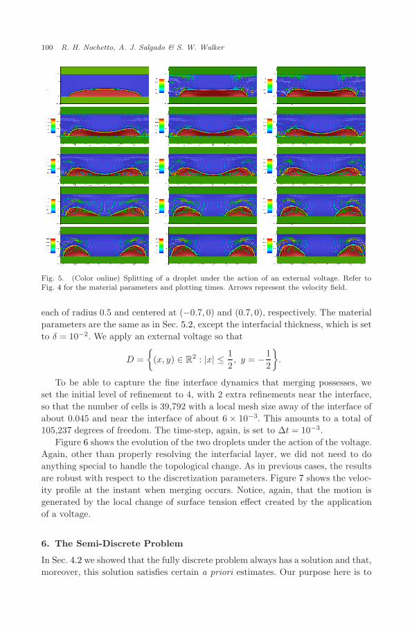
Fig. 5. (Color online) Splitting of a droplet under the action of an external voltage. Refer toFig. 4 for the material parameters and plotting times. Arrows represent the velocity field.
each of radius 0.5 and centered at (−0.7, 0) and (0.7, 0), respectively. The materialparameters are the same as in Sec. 5.2, except the interfacial thickness, which is setto δ = 10−2. We apply an external voltage so that
D =
(x, y) ∈ R2 : |x| ≤ 12, y = −1
2
.
To be able to capture the fine interface dynamics that merging possesses, weset the initial level of refinement to 4, with 2 extra refinements near the interface,so that the number of cells is 39,792 with a local mesh size away of the interface ofabout 0.045 and near the interface of about 6 × 10⁻³. This amounts to a total of105,237 degrees of freedom. The time-step, again, is set to ∆t = 10−3.
Figure 6 shows the evolution of the two droplets under the action of the voltage.Again, other than properly resolving the interfacial layer, we did not need to doanything special to handle the topological change. As in previous cases, the resultsare robust with respect to the discretization parameters. Figure 7 shows the veloc-ity profile at the instant when merging occurs. Notice, again, that the motion isgenerated by the local change of surface tension effect created by the applicationof a voltage.
6. The Semi-Discrete Problem
In Sec. 4.2 we showed that the fully discrete problem always has a solution and that,moreover, this solution satisfies certain a priori estimates. Our purpose here is to
October 23, 2013 15:48 WSPC/103-M3AS 1350047
Electrowetting 101
Fig. 6. (Color online) The material parameters are ρ1/ρ2 = 100, η1/η2 = 10, γ = 50, K1/K2 =10, ε1/ε2 = 5, εD/ε2 = 100, M = 10−2, α = 10−3, β = 10, θs = 120, δ = 10−2, λ = 0.5 andV00 = 20. The interface is shown at times 0, 1, 2, 3, 3.3, 3.4, 3.5, 4, 5 and 5.5. Colored lines are usedto represent the iso-values of the voltage. The black dotted line is the position of the interface atthe beginning of the computations.
October 23, 2013 15:48 WSPC/103-M3AS 1350047
102 R. H. Nochetto, A. J. Salgado & S. W. Walker
Fig. 7. (Color online) Merging of two droplets under the action of an externally applied voltage.Refer to Fig. 6 for material parameters. The interface is shown at the instant when merging occurs.Arrows represent the velocity field.
pass to the limit for h → 0 so as to show that a semi-discrete (that is continuousin space and discrete in time) version of our electrowetting model always has asolution.
Let us begin by defining the semi-discrete problem. Given initial data and anexternal voltage, we find:
Remark 6.1. (Permittivity) Notice that, in our definition of solution, the testfunction for Eq. (6.4) needs to be bounded. This is necessary to make sense of theterm
〈E(φn+1, φn)|∇V n+1|2, µ〉,
since E is bounded by construction and V n+1 ∈ H1(Ω). The authors of Ref. 27 useda similar choice of test functions and showed, using different techniques, existenceof a solution for their model of electrowetting in the case when the permittivity isphase-dependent.
Since the solution to the fully discrete problem (4.3)–(4.8) exists for all values ofh > 0 and satisfies uniform bounds, one expects the sequence of discrete solutions toconverge, in some topology, and that the limit is a solution of problem (6.1)–(6.5).The following result shows that this is indeed the case.
Theorem 6.1. (Existence and stability) For all ∆t > 0, problem (6.1)–(6.5) has asolution. Moreover, this solution satisfies an energy estimate, analogous to (4.11),where the constant c might depend on ∆t and the data of the problem, but not onthe solution.
Proof. Theorem 4.1 shows the existence, for every h > 0, of a solution to thefully discrete problem (4.3)–(4.8) which, moreover, satisfies estimate (4.11). Thisestimate implies that, for every n, as h→ 0:
• W(φnh) remains bounded in L1(Ω). Since the modified Ginzburg–Landau poten-
tial is a quadratic function of its argument, this implies that there is a subse-quence, again labeled by φn
h , that converges weakly in L2(Ω).• ∇φn
h remains bounded in L2. This, together with the previous observation, givesus a subsequence that converges weakly in H1(Ω) and strongly in L2(Ω).
• The strong L2-convergence of φnh implies that the convergence is almost every-
where and, since all the material functions are assumed continuous, the coeffi-cients also converge almost everywhere.
October 23, 2013 15:48 WSPC/103-M3AS 1350047
104 R. H. Nochetto, A. J. Salgado & S. W. Walker
• There is a subsequence of un+1h that converges weakly in V and strongly in L2(Ω).
• A subsequence of V nh − V n
0 converges weakly in H1 (Ω) and hence strongly in
L2(Ω).• There is a subsequence of qn+1
h that converges weakly in L2(Ω). Moreover, weknow that K(φn
h)∇(λqn+1h + V n+1
h ) converges weakly. By the a.e. convergence ofthe coefficients and the L2-weak convergence of ∇V n+1
h we conclude that ∇qn+1h
must converge weakly and, thus, the convergence is weak in H1(Ω) and strongin L2(Ω).
• The quantity φn+1h = dφn+1
h
∆t + un+1hτ ψ(φn
h) remains bounded in L2(Γ), whichimplies that there is a subsequence of φn+1
h that converges weakly in L2(Γ).• ∇µn
h remains bounded in L2(Ω). Moreover, setting µh = 1 in (4.6) and theobservations given above, imply
|〈µn+1h , 1〉| ≤
∣∣∣∣γδ 〈W ′(φkh) + Adφk+1
h , 1〉 +12〈ρ′(φn
h)unh ,u
n+1h 〉
+α[φk+1h , 1] + γ[Θ′
fs(φnh) + Bdφn+1
h , 1]∣∣∣∣ ≤ c,
which shows that∫Ωµn+1
h remains bounded and, thus, µnh remains bounded in
H1(Ω) and so there is a subsequence that converges weakly inH1(Ω) and stronglyin L2(Ω).
• Finally, we use the compatibility condition (4.2) and the discrete momentumEq. (4.8a) to obtain an estimate on the pressure pn+1
h ,
c‖pn+1h ‖L2 ≤ 1
∆t‖ρ(φn
h)‖L∞‖dun+1h ‖L2 +
1∆t
‖dρ(φn+1h )‖L∞‖un+1
h ‖L2
+ ‖ρ(φnh)‖L∞‖un
h‖H1‖un+1h ‖H1 + ‖ρ′(φn
h)‖L∞‖∇φnh‖L2
×‖unh‖H1‖un+1
h ‖H1 + ‖η(φnh)‖L∞‖S(un+1
h )‖L2
+ ‖β(φnh)‖L∞‖un+1
h ‖V + α‖ψ(φnh)‖L∞(Γ)‖φn+1
h ‖L2(Γ)
+ ‖µn+1h ‖H1‖∇φn
h‖L2 + ‖qn+1h ‖H1‖∇(λqn+1
h + V n+1h )‖L2
+1
∆t‖ρ′(φn
h)‖L∞‖dφn+1h ‖L2‖un
h‖V ≤ c
∆t,
which, for a fixed and positive ∆t, implies the existence of a L2-weakly convergentsubsequence.
It remains to show that this limit is a solution of (6.1)–(6.5):
Equation (6.1). Notice that if we show that, as h → 0, the sequence V n+1h con-
verges to V n+1 strongly in H1 (Ω), then the a.e. convergence of the coefficients
October 23, 2013 15:48 WSPC/103-M3AS 1350047
Electrowetting 105
implies
〈ε(φn+1h )∇V n+1
h ,∇W 〉Ω → 〈ε(φn+1)∇V n+1,∇W 〉Ω . (6.6)
Let us then show the strong convergence by an argument similar to that of [Ref. 27,p. 2778]. For any function V ∈ H1
(Ω), we introduce the elliptic projectionPhV ∈ Wh(V ) as the solution to
〈∇PhV,∇Wh〉Ω = 〈∇V,∇Wh〉Ω , ∀Wh ∈ Wh(0).
It is well known that PhV → V strongly in H1 (Ω). Given that ε is uniformly
bounded,
c‖∇(V n+1h − V n+1)‖2
L2 ≤ 〈ε(φn+1h )∇(V n+1
h − V n+1),∇(V n+1h − V n+1)〉Ω
= 〈ε(φn+1h )∇V n+1
h ,∇(PhVn+1 − V n+1)〉Ω
+ 〈ε(φn+1h )∇V n+1
h ,∇(V n+1h − PhV
n+1)〉Ω
+ 〈ε(φn+1h )∇V n+1,∇(V n+1 − V n+1
h )〉Ω
= I + II + III .
Let us estimate each of the terms separately. Since the coefficients are boundedand the sequence ∇V n+1
h is uniformly bounded in L2(Ω), the strong convergenceof PhV
n+1 shows that I → 0. For II we use the equation, namely
II = 〈ε(φn+1h )∇V n+1
h ,∇(V n+1h − PhV
n+1)〉Ω = 〈qn+1h , V n+1
h − PhVn+1〉 → 0
since qn+1h converges strongly in L2(Ω). Finally, notice that the last term can be
rewritten as
III = 〈(ε(φn+1h )]] − ε(φn+1)∇V n+1,∇(V n+1 − V n+1
h )〉Ω
+ 〈ε(φn+1)∇V n+1,∇(V n+1 − V n+1h )〉Ω .
The uniform boundedness of ∇V n+1h in L2(Ω) implies that, for the first term, it
suffices to show that (ε(φn+1h ) − ε(φn+1))∇V n+1 → 0 in L2(Ω), which follows
from the Lebesgue dominated convergence theorem. For the second term, use theweak convergence of ∇V n+1
h . This, together with the strong L2-convergence of qn+1h
implies that the limit solves (6.1).
Equation (6.2). The strong L2-convergence of qn+1h implies that 1
∆tdqn+1h →
1∆tdq
n+1 strongly in L2(Ω). Using the compact embeddings H1(Ω) L4(Ω) andV L4(Ω), we see that
〈qnhun+1
h ,∇r〉 → 〈qnun+1,∇r〉, ∀ r ∈ H1(Ω),
as h → 0. The term K(φnh)∇(λqn+1
h + V n+1h ) can be treated as in (6.6). These
observations imply that the limit solves (6.2).
October 23, 2013 15:48 WSPC/103-M3AS 1350047
106 R. H. Nochetto, A. J. Salgado & S. W. Walker
Equation (6.3). The strong L2-convergence of un+1h , the weak H1-convergence of
φn+1h and an argument similar to (6.6) imply that the limit solves (6.3).
Equation (6.4). The smoothness of W and the fact that its growth is quadraticimply
|〈W ′(φnh) −W ′(φn), µ〉| ≤ max
ϕ|W ′′(ϕ)|‖φn
h − φn‖L2‖µ‖L2 → 0.
A similar argument and the embedding H1(Ω) L2(Γ) can be used to show con-vergence of Θ′
fs(φnh). Since ρ is a bounded smooth function,
〈ρ′(φnh)un
h · un+1h , µ〉 → 〈ρ′(φn)un · un+1, µ〉.
The strong L2-convergence of ∇V n+1h implies that
〈E(φn+1h , φn
h)|∇V n+1h |2, µ〉 → 〈E(φn+1, φn)|∇V n+1|2, µ〉,
where it is necessary to have µ ∈ L∞(Ω). To conclude that (6.4) is satisfied bythe limit, it is left to show that φn+1
h converges strongly in L2(Γ). We know thatφn+1
h converges weakly in L2(Γ). On the other hand, 1∆tdφ
n+1h converges strongly
in L2(Γ),un+1hτ converges strongly in L2(Γ) and ψ(φn
h) converges a.e. in Γ.
Equations (6.5). Clearly, (6.5b) is satisfied. To show that (6.5a) holds, notice that
〈ρ(φn+1h )un+1
h − ρ(φn+1)un+1,w〉
= 〈ρ(φn+1h )(un+1
h − un+1),w〉 + 〈(ρ(φn+1h ) − ρ(φn+1))un+1,w〉 → 0.
Since we assume that ψ is smooth and the slip coefficient β is smooth and dependsonly on the phase field, but not on the stress (as opposed to Sec. 2.4), we can getconvergence of the terms [β(φn
h)un+1hτ ,wτ ] and [un+1
hτ ψ(φnh),wτψ(φn
h)], respectively.The advection term can be treated using standard arguments and thus we will notgive details here. The terms
〈µn+1h ∇φn
h,w〉, 〈qnh∇(λqn+1
h + V n+1h ),∇w〉,
can be treated using arguments similar to the ones given before. The term⟨ρ′(φn
h)dφn+1
h
∆tun
h,w⟩,
can be easily shown to converge since all terms converge strongly. The convergenceof the term [
dφn+1h
∆t,wτψ(φn
h)],
follows again from the compact embeddingH1(Ω) L2(Γ). Finally, the convergenceof the viscous stress term follows the lines of the proof of (6.6).
To conclude, we notice that we do not need to reprove estimates similar to (4.11).These are uniformly valid, in h, for all terms in the sequence and, therefore, valid
October 23, 2013 15:48 WSPC/103-M3AS 1350047
Electrowetting 107
for the limit. Moreover, if one wanted to obtain an energy estimate by repeatingthe arguments used to obtain Proposition 4.1 it would be necessary first to obtainuniform L∞ bounds on the sequence dφh,∆t, since one of the steps in the proofrequires setting µh = 2dφn+1
h .
Remark 6.2. (Limit ∆t → 0) We are unable to pass to the limit when ∆t → 0for several reasons. First, the estimates on the pressure depend on the time-stepand getting around this would require finer estimates on the time derivative of thevelocity, this is standard for Navier–Stokes. In addition, the terms⟨
ρ′(φn)dφn+1
∆tun,w
⟩,
⟨dρ(φn+1)
∆tun+1,w
⟩,
would require finer estimates on the time derivative of the phase field which wehave not been able to show. It might be possible, however, to circumvent thesetwo restrictions by defining the weak solution to the continuous problem with anunconstrained formulation for the momentum equation (i.e. solution and test func-tions in V) and modifying the Cahn–Hilliard equations to their “viscous version”,in other words suitably adding a term of the form φt. We will not pursue thisdirection.
7. Conclusions and Perspectives
Some possible directions for future work would be to extend the analysis by passingto the limit as ∆t → 0, or investigate the phenomenological pinning model morethoroughly. It would also be interesting to look at the use of open boundary con-ditions on ∂Ω, which is more physically correct for some electrowetting devices.As far as we know, this is an open area of research in the context of phase-fieldmethods. Other extensions of the model could include the transport of surfactant atthe liquid–gas interface, though this would make the model more complicated. Wewant to emphasize that our model gives physically reasonable results when mod-eling actual electrowetting systems, and so could be used within an optimizationframework for improving device design.
Concerning numerics, an important issue that has not been addressed is howto actually solve the discretized systems. Even in the fully uncoupled case, thepresence of the dynamic boundary condition in the Cahn–Hilliard system (Step 2in the scheme of Sec. 5) makes this problem extremely ill-conditioned and standardpreconditioning techniques (for instance the one in Ref. 10) inapplicable.
Acknowledgments
This material is based on work supported by NSF grants CBET-0754983 and DMS-0807811. A.J.S. is also supported by an AMS-Simons Grant.
October 23, 2013 15:48 WSPC/103-M3AS 1350047
108 R. H. Nochetto, A. J. Salgado & S. W. Walker
References
1. H. Abels, H. Garcke and G. Grun, Thermodynamically consistent, frame indifferentdiffuse interface models for incompressible two-phase flows with different densities,Math. Models Methods Appl. Sci. 22 (2012) 1150013.
2. R. A. Adams and J. J. F. Fournier, Sobolev Spaces, 2nd edn., Pure and AppliedMathematics, Vol. 140 (Academic Press, 2003).
3. H. W. Alt, The entropy principle for interfaces. Fluids and solids, Adv. Math. Sci.Appl. 19 (2009) 585–663.
4. H. Aminfar and M. Mohammadpourfard, Lattice Boltzmann method for electrowet-ting modeling and simulation, Comput. Methods Appl. Mech. Engrg. 198 (2009)3852–3868.
5. H. Aminfar and M. Mohammadpourfard, Lattice Boltzmann simulation of dropletbase electrowetting, Int. J. Comput. Fluid Dyn. 24 (2010) 143–156.
6. D. M. Anderson, G. B. McFadden and A. A. Wheeler, Diffuse-interface methods influid mechanics, Annu. Rev. Fluid Mech. 30 (1998) 139–165.
7. D. Aronov, M. Molotskii and G. Rosenman, Electron-induced wettability modifica-tion, Phys. Rev. B 76 (2007) 035437.
8. W. Bangerth, R. Hartmann and G. Kanschat, deal. II Differential Equations AnalysisLibrary, Technical Reference, http://www.dealii.org.
9. W. Bangerth, R. Hartmann and G. Kanschat, deal. II — A general-purpose object-oriented finite element library, ACM Trans. Math. Softw. 33 (2007) 24/1–24/7.
10. E. Bansch, P. Morin and R. H. Nochetto, Preconditioning a class of fourth orderproblems by operator splitting, Numer. Math. 118 (2011) 197–228.
11. B. Berge, Electrocapillarite et mouillage de films isolants par l’eau (including anenglish translation), C. R. Acad. Sci. Paris, Ser. II 317 (1993) 157–163.
12. B. Berge and J. Peseux, Variable focal lens controlled by an external voltage: Anapplication of electrowetting, Euro. Phys. J. E 3 (2000) 159–163.
13. J. Billingham, On a model for the motion of a contact line on a smooth solid surface,Euro. J. Appl. Math. 17 (2006) 347–382.
14. J. Billingham, Gravity-driven thin-film flow using a new contact line model, IMA J.Appl. Math. 73 (2008) 4–36.
15. F. Boyer, Nonhomogeneous Cahn–Hilliard fluids, Ann. Inst. H. Poincare Anal. NonLineaire 18 (2001) 225–259.
16. F. Boyer, A theoretical and numerical model for the study of incompressible mixtureflows, Computers & Fluids 31 (2002) 41–68.
17. F. Boyer, C. Lapuerta, S. Minjeaud, B. Piar and M. Quintard, Cahn–Hilliard/Navier–Stokes model for the simulation of three-phase flows, Transp. Porous Media 82 (2010)463–483.
18. F. Brezzi and M. Fortin, Mixed and Hybrid Finite Element Methods (Springer-Verlag,1991).
19. G. C. Buscaglia and R. F. Ausas, Variational formulations for surface tension, capil-larity and wetting, Computer Methods Appl. Mech. Engrg. 200 (2011) 3011–3025.
20. L. A. Caffarelli and N. E. Muler, An L∞ bound for solutions of the Cahn–Hilliardequation, Arch. Rational Mech. Anal. 133 (1995) 129–144.
21. L. Cherfils, M. Petcu and M. Pierre, A numerical analysis of the Cahn–Hilliardequation with dynamic boundary conditions, Disc. Contin. Dyn. Syst. 27 (2010)1511–1533.
22. S. K. Cho, H. Moon, J. Fowler, S.-K. Fan and C.-J. Kim, Splitting a liquid droplet forelectrowetting-based microfluidics, in International Mechanical Engineering Congressand Exposition (ASME Press, 2011).
October 23, 2013 15:48 WSPC/103-M3AS 1350047
Electrowetting 109
23. S. K. Cho, H. Moon and C.-J. Kim, Creating, transporting, cuttingand merging liquiddroplets by electrowetting-based actuation for digital microfluidic circuits, J. Micro-electromech. Syst. 12 (2003) 70–80.
24. P. Ciarlet, Jr. and C. Scheid, Electrowetting of a 3D drop: Numerical modelling withelectrostatic vector fields, M2AN Math. Model. Numer. Anal. 44 (2010) 647–670.
25. P. G. Ciarlet, The Finite Element Method for Elliptic Problems (North-Holland, 1978).26. F. Klingbeil, E. Campillo-Funollet and G. Grun, On modeling and simulation of elec-
trokinetic phenomena in two-pahse flow with general mass densities, in preparation,2011.
27. C. Eck, M. Fontelos, G. Grun, F. Klingbeil and O. Vantzos, On a phase-field modelfor electrowetting, Interfaces Free Bound. 11 (2009) 259–290.
28. A. Ern and J.-L. Guermond, Theory and Practice of Finite Elements, Applied Math-ematical Sciences, Vol. 159 (Springer-Verlag, 2004).
29. L. C. Evans, Partial Differential Equations, Graduate Studies in Mathematics, Vol. 19(Amer. Math. Soc., 1998).
30. M. A. Fontelos, G. Grun and S. Jorres, On a phase-field model for electrowetting andother electrokinetic phenomena, SIAM J. Math. Anal. 43 (2011) 527–563.
31. M. A. Fontelos and U. Kindelan, A variational approach to contact angle saturationand contact line instability in static electrowetting, Quart. J. Mech. Appl. Math.62 (2009) 465–479.
32. J.-F. Gerbeau and T. Lelievre, Generalized Navier boundary condition and geometricconservation law for surface tension, Comput. Methods Appl. Mech. Engrg. 198 (2009)644–656.
33. V. Girault and P.-A. Raviart, Finite Element Methods for Navier–Stokes Equations.Theory and Algorithms, Springer Series in Computational Mathematics (Springer-Verlag, 1986).
34. H. Gomez and T. J. R. Hughes, Provably unconditionally stable, second-ordertime-accurate, mixed variational methods for phase-field models, J. Comput. Phys.230 (2011) 5310–5327.
35. J. Gong, S. K. Fan and C. J. Kim, Portable digital microfluidics platform with activebut disposable lab-on-chip, in 17th IEEE Int. Conf. Micro Electro Mechanical Systems(MEMS) (IEEE Press, 2004), pp. 355–358.
36. G. Grun and F. Klingbeil, Two-phase flow with mass density contrast: Stable schemesfor a thermodynamic consistent and frame-indifferent diffuse interface model, inpreparation.
37. J.-L. Guermond and L. Quartapelle, A projection FEM for variable density incom-pressible flows, J. Comput. Phys. 165 (2000) 167–188.
38. J.-L. Guermond and A. Salgado, A splitting method for incompressible flows withvariable density based on a pressure Poisson equation, J. Comput. Phys. 228 (2009)2834–2846.
39. F. Guillen-Gonzalez and J. V. Gutierrez-Santacreu, Unconditional stability and con-vergence of fully discrete schemes for 2D viscous fluids models with mass diffusion,Math. Comput. 77 (2008) 1495–1524.
40. R. A. Hayes and B. J. Feenstra, Video-speed electronic paper based on electrowetting,Nature 425 (2003) 383–385.
41. D. Jacqmin, Contact-line dynamics of a diffuse fluid interface, J. Fluid Mech.402 (2000) 57–88.
42. D. Kamiya and M. Horie, Electrowetting on silicon single-crystal substrates, ContactAngle, Wettability and Adhesion 2 (2002) 507–520.
43. F. Klingbeil, On convergent schemes for dynamic electrowetting, in preparation.
October 23, 2013 15:48 WSPC/103-M3AS 1350047
110 R. H. Nochetto, A. J. Salgado & S. W. Walker
44. T. Krupenkin and J. A. Taylor, Reverse electrowetting as a new approach to high-power energy harvesting, Nat. Commun. 2 (2011) 2011/08/23/online.
45. J. Lee, H. Moon, J. Fowler, T. Schoellhammer and C.-J. Kim, Electrowetting andelectrowetting-on-dielectric for microscale liquid handling, Sensors and Actuators, A-Phys. 95 (2002) 259–268.
46. Ed. D. R. Lide, Handbook of Chemistry and Physics, 82nd edn. (CRC Press, 2002).47. G. Lippmann, Relations entre les phenomenes electriques et capillaires, Ann. Chim.
Phys. 5 (1875) 494–549.48. C. Liu and J. Shen, A phase field model for the mixture of two incompressible fluids
and its approximation by a Fourier-spectral method, Phys. D 179 (2003) 211–228.49. H.-W. Lu, K. Glasner, A. L. Bertozziand and C.-J. Kim, A diffuse-interface model for
electrowetting drops in a Hele–Shaw cell, J. Fluid Mech. 590 (2007) 411–435.50. J. Monnier, A. M. Benselama and I. Cotoi, Flow patterns in the vicinity of triple
line dynamics arising from a local surface tension model, Int. J. Multiscale Comput.Engrg. 5 (2007) 417–434.
51. J. Monnier, P. Witomski, P. Chow-Wing-Bom and C. Scheid, Numerical model-ing of electrowetting by a shape inverse approach, SIAM J. Appl. Math. 69 (2009)1477–1500.
52. F. Mugele and J. Baret, Electrowetting: From basics to applications, J. Phys.: Con-dens. Matter 17 (2005) R705–774.
53. L. Onsager, Reciprocal relations in irreversible processes. I, Phys. Rev. 37 (1931)405–426.
54. A. Prohl and M. Schmuck, Convergent discretizations for the Nernst–Planck–Poissonsystem, Numer. Math. 111 (2009) 591–630.
55. A. Prohl and M. Schmuck, Convergent finite element for discretizations of the Navier–Stokes–Nernst–Planck–Poisson system, M2AN Math. Model. Numer. Anal. 44 (2010)531–571.
56. J. Pruss, R. Racke and S. Zheng, Maximal regularity and asymptotic behavior ofsolutions for the Cahn–Hilliard equation with dynamic boundary conditions, Ann.Mat. Pura Appl. (4 ) 185 (2006) 627–648.
57. T. Qian, X.-P. Wang and P. Sheng, Molecular hydrodynamics of the moving contactline in two-phase immiscible flows, Commun. Comput. Phys. 1 (2006) 1–52.
58. T. Qian, X.-P. Wang and P. Sheng, A variational approach to moving contact linehydrodynamics, J. Fluid Mech. 564 (2006) 333–360.
59. T. Roques-Carmes, R. A. Hayes, B. J. Feenstra and L. J. M. Schlangen, Liquid behav-ior inside a reflective display pixel based on electrowetting, J. Appl. Phys. 95 (2004)4389–4396.
60. T. Roques-Carmes, R. A. Hayes, B. J. Feenstra and L. J. M. Schlangen, A physicalmodel describing the electro-optic behavior of switchable optical elements based onelectrowetting, J. Appl. Phys. 96 (2004) 6267–6271.
61. F. Saeki, J. Baum, H. Moon, J.-Y. Yoon, C.-J. Kim and R. L. Garrell, Electrowettingon dielectrics (ewod): Reducing voltage requirements for microfluidics, Polym. Mater.Sci. Engrg. 85 (2001) 12–13.
62. A. J. Salgado, A diffuse interface fractional time-stepping technique for incompressibletwo-phase flows with moving contact lines, M2AN Math. Model. Numer. Anal. (2012),DOI:10.1051/m2an/2012047.
63. A. J. Salgado, A general framework for the implementation of multiphysics and mul-tidomain problems using the deal.II library, Arch. Numer. Softw. 2012, accepted.
64. C. Scheid and P. Witomski, A proof of the invariance of the contact angle in elec-trowetting, Math. Comput. Model. 49 (2009) 647–665.
October 23, 2013 15:48 WSPC/103-M3AS 1350047
Electrowetting 111
65. M. Schmuck, Analysis of the Navier–Stokes–Nernst–Planck–Poisson system, Math.Models Methods Appl. Sci. 19 (2009) 993–1015.
66. B. Shapiro, H. Moon, R. Garrell and C.-J. Kim, Equilibrium behavior of sessile dropsunder surface tension, applied external fieldsand material variations, J. Appl. Phys.93 (2003) 5794–5811.
67. J. Shen and X. Yang, Energy stable schemes for Cahn–Hilliard phase-field model oftwo-phase incompressible flows, Chin. Ann. Math. Ser. B 31 (2010) 743–758.
68. J. Shen and X. Yang, Numerical approximations of Allen–Cahn and Cahn–Hilliardequations, Disc. Contin. Dyn. Syst. 28 (2010) 1669–1691.
69. J. Shen and X. Yang, A phase-field model and its numerical approximation for two-phase incompressible flows with different densities and viscosities, SIAM J. Sci. Com-put. 32 (2010) 1159–1179.
70. Y. D. Shikhmurzaev, The moving contact line on a smooth solid surface, Int. J.Multiphase Flow 19 (1993) 589–610.
71. Y. D. Shikhmurzaev, Capillary Flows with Forming Interfaces (Chapman &Hall/CRC, 2008).
72. J. Song, R. Evans, Y.-Y. Lin, B.-N. Hsu and R. Fair, A scaling model forelectrowetting-on-dielectric microfluidic actuators, Microfluidics and Nanofluidics7 (2009) 75–89.
73. S. W. Walker, A. Bonito and R. H. Nochetto, Mixed finite element method for elec-trowetting on dielectric with contact line pinning, Interfaces Free Bound. 12 (2010)85–119.
74. S. W. Walker, B. Shapiro and R. H. Nochetto, Electrowetting with contact linepinning: Computational modeling and comparisons with experiments, Phys. Fluids21 (2009) 102103.
75. S. M. Wise, C. Wang and J. S. Lowengrub, An energy-stable and convergentfinite-difference scheme for the phase field crystal equation, SIAM J. Numer. Anal.47 (2009) 2269–2288.
76. E. Zeidler, Nonlinear Functional Analysis and its Applications. I (Springer-Verlag,1986). Fixed-point theorems, Translated from German by Peter R. Wadsack.