Queueing Systems 50, 371–400, 2005 c 2005 Springer Science + Business Media, Inc. Manufactured in The Netherlands. A Diffusion Approximation for a GI/GI/1 Queue with Balking or Reneging AMY R. WARD [email protected]School of Industrial and Systems Engineering, Georgia Institute of Technology, Atlanta, GA 30332-0205, USA PETER W. GLYNN [email protected]Department of Management Science & Engineering, Stanford University, Stanford, CA 94305, USA Received 31 October 2003; Revised 7 January 2005 Abstract. Consider a single-server queue with a renewal arrival process and generally distributed processing times in which each customer independently reneges if service has not begun within a generally distributed amount of time. We establish that both the workload and queue-length processes in this system can be approximated by a regulated Ornstein-Uhlenbeck (ROU) process when the arrival rate is close to the processing rate and reneging times are large. We further show that a ROU process also approximates the queue-length process, under the same parameter assumptions, in a balking model. Our balking model assumes the queue-length is observable to arriving customers, and that each customer balks if his or her conditional expected waiting time is too large. Keywords: deadlines, reneging, balking, impatience, GI/GI/1-GI queue, Ornstein-Uhlenbeck process, regulated diffusion, reflected diffusion 1. Introduction Queueing models in which customers may renege, or abandon the system before receiv- ing service, arise in many diverse applications domains. For example, in the multi-billion dollar call center industry, impatient customers often hang-up before reaching a service agent. Furthermore, in the manufacturing context, customer order cancellation was one factor in the $2.2 billion component inventory write-off of Cisco Systems in the third quarter of 2001 [2]. Finally, in the networking context, certain packets of data (for ex- ample, location data in wireless networks) lose their value unless transmitted or received within a given time interval. In the case of a call center, it is tempting to assume a purely exponential model. However, the work of Brown et al. [5] that analyzes a data set consisting of over 1,200,000 calls to a bank call center concludes that service times follow a lognormal distribution and reneging times are not exponential. Hence it is desirable to obtain performance
A Diffusion Approximation for a GI/GI/1 Queuewith Balking or Reneging
AMY R. WARD [email protected] of Industrial and Systems Engineering, Georgia Institute of Technology, Atlanta,GA 30332-0205, USA
PETER W. GLYNN [email protected] of Management Science & Engineering, Stanford University, Stanford, CA 94305, USA
Received 31 October 2003; Revised 7 January 2005
Abstract. Consider a single-server queue with a renewal arrival process and generally distributed processingtimes in which each customer independently reneges if service has not begun within a generally distributedamount of time. We establish that both the workload and queue-length processes in this system can beapproximated by a regulated Ornstein-Uhlenbeck (ROU) process when the arrival rate is close to theprocessing rate and reneging times are large. We further show that a ROU process also approximates thequeue-length process, under the same parameter assumptions, in a balking model. Our balking modelassumes the queue-length is observable to arriving customers, and that each customer balks if his or herconditional expected waiting time is too large.
Queueing models in which customers may renege, or abandon the system before receiv-ing service, arise in many diverse applications domains. For example, in the multi-billiondollar call center industry, impatient customers often hang-up before reaching a serviceagent. Furthermore, in the manufacturing context, customer order cancellation was onefactor in the $2.2 billion component inventory write-off of Cisco Systems in the thirdquarter of 2001 [2]. Finally, in the networking context, certain packets of data (for ex-ample, location data in wireless networks) lose their value unless transmitted or receivedwithin a given time interval.
In the case of a call center, it is tempting to assume a purely exponential model.However, the work of Brown et al. [5] that analyzes a data set consisting of over 1,200,000calls to a bank call center concludes that service times follow a lognormal distributionand reneging times are not exponential. Hence it is desirable to obtain performance
372 WARD AND GLYNN
measure approximations for queueing models with reneging in the most general frame-work possible.
The main contribution of this paper is to show that a regulated Ornstein-Uhlenbeck(ROU) process plays a similar role in the context of queues with reneging or balking asdoes regulated Brownian motion (RBM) in the setting of conventional queues. Specifi-cally, we show that a ROU arises as a heavy traffic diffusion limit for the queue-lengthand workload processes when the customer arrival rate is close to the service rate andreneging times are large; see Theorems 1, 2, 3, and 4. This extends the work of Wardand Glynn [23], where heavy-traffic limits for a single-server queue with reneging weredeveloped in a purely exponential setting.
We develop our limit theorems via a result for the offered waiting time process.The offered waiting time process consists of the workload of all customers in the queuethat will eventually reach the server. This process differs from the observed workloadprocess, which consists of the workload of all customers in the queue—regardless ofwhether or not they eventually renege. We show that the behavior of both of theseprocesses is identical in the heavy-traffic diffusion limit; see Theorems 1 and 2.
Our limit theorems show the behavior of the derivative of the deadline distributionfunction at the point zero is important. In particular, it is this value that controls thestrength of the linear state-dependence in the limiting ROU process.
The remainder of this paper is organized as follows. We conclude this sectionwith a review of relevant literature. In Section 2, we formulate our balking and renegingmodels, and provide stability conditions. In Section 3, we establish the weak convergenceof the diffusion scaled offered waiting time and workload processes. We then show theweak convergence of the diffusion scaled queue-length processes in both our renegingand balking models in Section 4. Finally, in Section 5, we provide a simulation studyshowing the mean of an appropriate ROU process provides a good approximation to thesteady-state mean queue-length in a reneging or balking model.
1.1. Literature review
Palm [18] introduced reneging as a means of modeling the behavior of telephone switch-board customers more than 60 years ago. Later, for a purely exponential model, Anckerand Gafarian [3] explicitly computed stationary probabilities for the number of cus-tomers in the system. Such explicit expressions are not possible for GI/GI/1 modelswith generally distributed reneging times. It is true that expressions for many steady-state performance measures of interest can be written in terms of the limiting distributionof the work seen by an arbitrary arrival to the system (assuming the limit distributionexists); see Stanford [22] and Baccelli, Boyer, and Hebuterne [4]. However, this limitdistribution is given in the form of an integral equation, which may be difficult to solve.
The situation for obtaining explicit expressions for transient performance mea-sures is hopeless. Even for purely exponential models, computations for transient per-formance measures generally involve numerical procedures to invert transforms, asshown in Whitt [25]. Hence it is desirable to develop diffusion approximations (with
GI/GI/1 GI QUEUES 373
analytically tractable steady-state and transient behavior) for the queue-length and work-load processes in systems with reneging. Ward and Glynn [23] show a ROU process wellapproximates an M/M/1 queue with exponential reneging when the arrival rate is close tothe processing rate and the reneging rate is small. For a queue with many servers, Poissonarrivals, and exponential processing and reneging, Garnett, Mandelbaum, and Reiman[12] develop a different diffusion approximation as the number of servers grows largein the Halfin-Whitt regime. For a many server queue with a general reneging distribu-tion having Poisson arrivals and exponential processing times, Mandelbaum and Zeltyn[17] analyze the robustness of a linear relationship between customer abandonmentprobability and average waiting time observed in telephone call center data.
For models with general distributions, Coffman, Puhalskii, Reiman, and Wright[9] conjecture the appropriate diffusion limit for a system with reneging operating un-der a processor-sharing discipline when the arrival rate is large. Doytchinov, Lehoczky,and Shreve [10] establish the heavy traffic limit for a GI/GI/1 system with generallydistributed customer reneging times operating under the earliest-deadline-first queuediscipline. In the case of constant deadlines (but a renewal arrival process and gen-eral service time distribution), Plambeck, Kumar, and Harrison [19], devise input andscheduling controls that are asymptotically optimal in the heavy-traffic limit regime.
2. Balking and reneging models
Our goal in this paper is to develop performance measure approximations for a classof GI/GI/1 queueing models with either reneging or balking. For all our models, weassume the server works at rate 1 under the FIFO discipline. The model primitives arethree independent sequences of non-negative, mean 1, i.i.d. random variables {ui : i ≥1}, {vi : i ≥ 1} and {wi : i ≥ 1}, which are all defined on a common probability space(�,F, P). For a given inter-arrival rate ρ and mean deadline time m, the inter-arrivaltime between the (i −1)st and i th customer is ρ−1ui , the service time of the ith customeris vi , and the maximum time the customer will wait for processing is di ≡ mwi . Fort > 0, the renewal process
A(t) = max{i ≥ 0 : u1 + · · · + ui ≤ ρt}
represents the cumulative number of arrivals in the first t time units, while the renewalprocess
S(t) = max{i ≥ 0 : v1 + · · · + vi ≤ t}
represents the number of customers processed in the first t units of server busy time.
374 WARD AND GLYNN
2.1. Evolution equations
In our reneging model, all customers initially join the queue. However, if the ith customer,who arrives at time
ti ≡i∑
j=1
ρ−1u j ,
must wait longer than di time units to reach the server, he departs at time ti + di withoutreceiving service. As observed by Baccelli, Boyer, and Hebuterne [4], for such a system,the time a served customer waits for service depends only on the processing times ofthe “non-reneging” customers in the queue at his arrival time. In other words, customersthat eventually renege from the queue do not contribute to the delay served customersexperience. We track the waiting time an arriving customer would experience at timet > 0 using the offered waiting time process
V (t) =A(t)∑
i=1
vi 1{V (t−i ) < di } − B(t), (2.1)
where B(t) ≡ ∫ t0 1{V (s) > 0}ds is the cumulative busy time.
The offered waiting time process differs from the process that measures the totalprocessing time of all the customers in the system at each point in time. We call thisprocess the observed workload process and define it to be
W (t) = V (t) +A(t)∑
i=1
vi 1{V (t−i ) ≥ di and ti ≤ t < ti + di }. (2.2)
We also desire to track the number of customers in the system over time, includingboth reneging and non-reneging customers. By looking at the offered waiting timeprocess at each customer arrival time, we can count the cumulative number of arrivalsthat eventually receive service,
∑A(t)i=1 1{V (t−
i ) < di }, and the number of customerscurrently in queue that eventually renege,
∑A(t)i=1 1{V (t−
i ) < di and ti ≤ t < ti + di }.Counting the cumulative number of departing customers requires more work becauseprocessing times are associated with customers, and so we must first determine theindices of served jobs. Let π (i) denote the index of the ith served job for i ≥ 1. Thesystem starts empty so that π (1) = 1. For i ≥ 2 we define π (i) recursively as
π (i) = min{n > π (i − 1) : V (t−n ) < dn}.
Then, the cumulative number of departures that have received service before time t is
S(t) = max
{i ≥ 0 :
i∑
j=1
vπ ( j) ≤ t
}.
GI/GI/1 GI QUEUES 375
Finally, the queue-length at time t is
Q(t) =A(t)∑
i=1
1{V (t−i ) < di } +
A(t)∑
i=1
1{V (t−i ) ≥ di and ti ≤ t < ti + di } − S(B(t)).
(2.3)
The offered waiting time process also arises as the workload process for a systemin which each customer balks if at his arrival time the offered waiting time exceeds hisdeadline. Such a balking assumption is realistic for models in which the processing timeof each customer in the queue is known. However, customer processing times often arenot observable, meaning the above balking model does not apply. In the case that queuelengths are observable (but customer processing times are not), one reasonable balkingmodel formulation assumes each customer joins the queue if the customer’s conditionalexpected waiting time at his arrival time exceeds his deadline. The queue-length processin this system is
Q B(t) =A(t)∑
i=1
1{Q B(t−i ) − 1 < di } − S(BB(t)), (2.4)
where BB(t) = ∫ t0 1{Q B(s) > 0}ds is the cumulative busy time in the balking system.
It is useful for our analysis to represent the offered waiting time process in termsof a stochastic integral and the following two martingales:
{(Mv(i) ≡
i∑
j=1
(v j − 1)1{V (t−j ) < d j },Fi
), i ≥ 0
}
and{(
Md(i) ≡i∑
j=1
1{V (t−j ) ≥ d j } − E[1{V (t−
j ) ≥ d j } |F j−1],Fi
), i ≥ 0
},
where
Fi = σ ((u1, v1, w1), . . . (ui , vi , wi ), ui+1) ⊂ F .
Our definition of Fi implies
P(V (t−i ) ≥ di |Fi−1) = F
(V (t−
i )
m
), i = 1, 2, . . . ,
376 WARD AND GLYNN
almost surely, where F is the cdf of w1, because V (t−i ) is Fi−1-measurable and wi is
independent of Fi−1. A little algebra shows
V (t) +A(t)∑
i=1
F
(V (t−
i )
m
)= A(t) + Mv(A(t)) − Md(A(t)) − t + I (t),
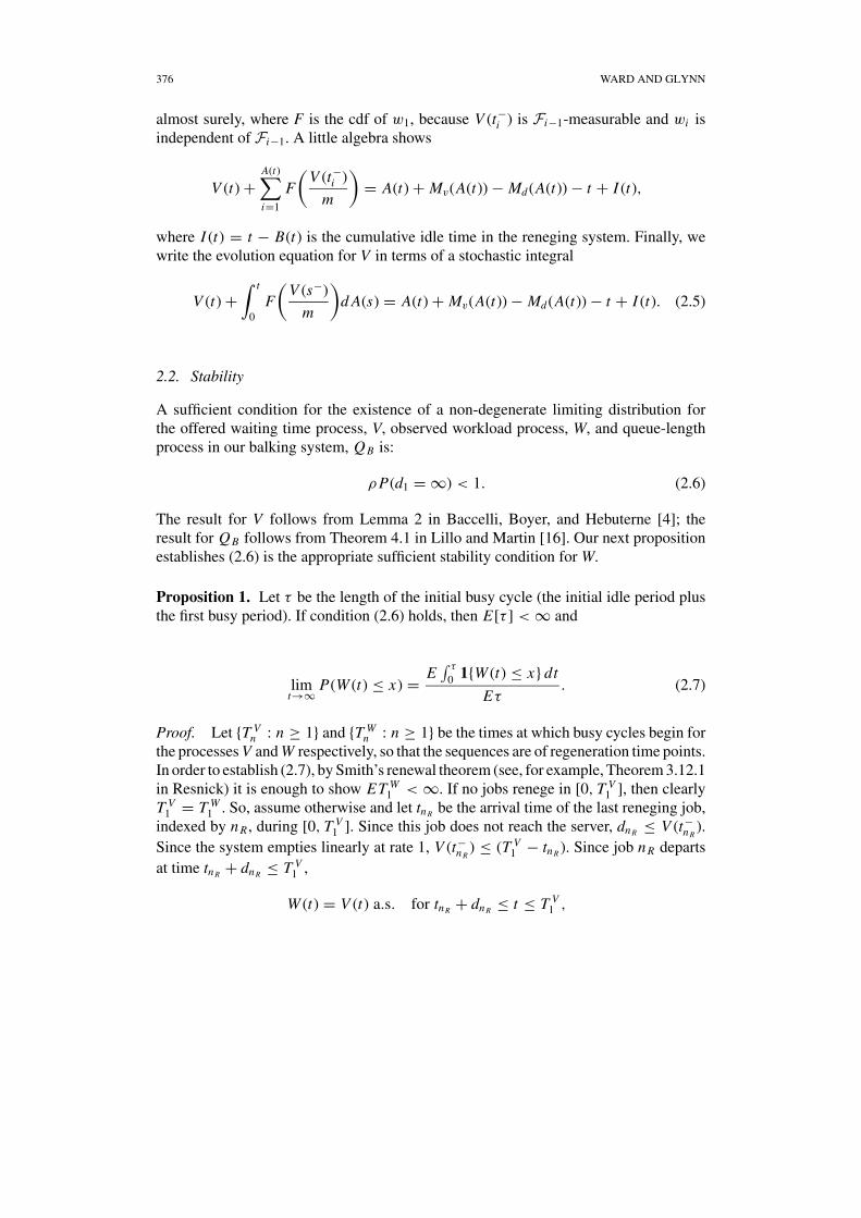
where I (t) = t − B(t) is the cumulative idle time in the reneging system. Finally, wewrite the evolution equation for V in terms of a stochastic integral
V (t) +∫ t
0F
(V (s−)
m
)d A(s) = A(t) + Mv(A(t)) − Md(A(t)) − t + I (t). (2.5)
2.2. Stability
A sufficient condition for the existence of a non-degenerate limiting distribution forthe offered waiting time process, V, observed workload process, W, and queue-lengthprocess in our balking system, Q B is:
ρ P(d1 = ∞) < 1. (2.6)
The result for V follows from Lemma 2 in Baccelli, Boyer, and Hebuterne [4]; theresult for Q B follows from Theorem 4.1 in Lillo and Martin [16]. Our next propositionestablishes (2.6) is the appropriate sufficient stability condition for W.
Proposition 1. Let τ be the length of the initial busy cycle (the initial idle period plusthe first busy period). If condition (2.6) holds, then E[τ ] < ∞ and
limt→∞ P(W (t) ≤ x) = E
∫ τ
0 1{W (t) ≤ x} dt
Eτ. (2.7)
Proof. Let {T Vn : n ≥ 1} and {T W
n : n ≥ 1} be the times at which busy cycles begin forthe processes V and W respectively, so that the sequences are of regeneration time points.In order to establish (2.7), by Smith’s renewal theorem (see, for example, Theorem 3.12.1in Resnick) it is enough to show ET W
1 < ∞. If no jobs renege in [0, T V1 ], then clearly
T V1 = T W
1 . So, assume otherwise and let tnR be the arrival time of the last reneging job,indexed by nR , during [0, T V
1 ]. Since this job does not reach the server, dnR ≤ V (t−nR
).Since the system empties linearly at rate 1, V (t−
nR) ≤ (T V
1 − tnR ). Since job nR departsat time tnR + dnR ≤ T V
1 ,
W (t) = V (t) a.s. for tnR + dnR ≤ t ≤ T V1 ,
GI/GI/1 GI QUEUES 377
which guarantees T V1 = T W
1 a.s. The consequences of Lemma 2 in Baccelli, Boyer,and Heburterne [4] detailed in Section 3.2 guarantee ET V
1 < ∞, and so ET W1 < ∞
also.
2.3. Heavy traffic conditions
Because obtaining closed-form expressions for performance measures in our balkingand reneging models appears impossible, we perform an asymptotic analysis in heavytraffic. We consider a sequence of systems, indexed by n, in which the arrival rate isρn and mean deadline lengths are mn . Any process or quantity associated with the nthsystem we superscript by n. Then, the random variable dn
i that represents the maximumtime a customer will wait for processing in the nth system has cdf
Fn(x) ≡ P(dn
i ≤ x) = P
(wi ≤ x
mn
)= F
(x
mn
).
Our analysis requires the following assumptions.
Assumption 1 (Heavy Traffic Requirements).
(a) As n → ∞,√
n(ρn − 1) → c, where c is a finite constant.
(b) The variances var(u1) and var(v1) are finite.
(c) The cdf F used to determine a particular customer’s deadline is differentiable about0, and F ′
d(0) < ∞.
We also state the following technicalities. All random variables are defined ona common probability space (�,F, P). Let D([0, ∞), ) be the space of right con-tinuous functions with left limits (RCLL) in having time domain [0, ∞). We en-dow D([0, ∞), ) with the usual Skorokhod J1 topology, and let M denote the Borelσ -algebra associated with the J1 topology. All stochastic processes are measurablefunctions from (�,F, P) into (D([0, ∞), ), M). Suppose {ξ n}∞n=1 is a sequence ofstochastic processes. The notation ξ n ⇒ ξ means that the probability measures in-duced by the ξ n’s on (D([0, ∞), ), M) converge weakly to the probability measure on(D([0, ∞), ), M) induced by the stochastic process ξ . For x ∈ (D([0, ∞), ), M) andt > 0, let
‖x‖t ≡ sup0≤s≤t
|x(s)|
be the uniform norm and note that ξ n converges almost surely (a.s.) to a continuous limitprocess ξ in the J1 topology if and only if the convergence is uniform on compact sets(u.o.c.)
‖ξ n − ξ‖t → 0 a.s.
for every t > 0.
378 WARD AND GLYNN
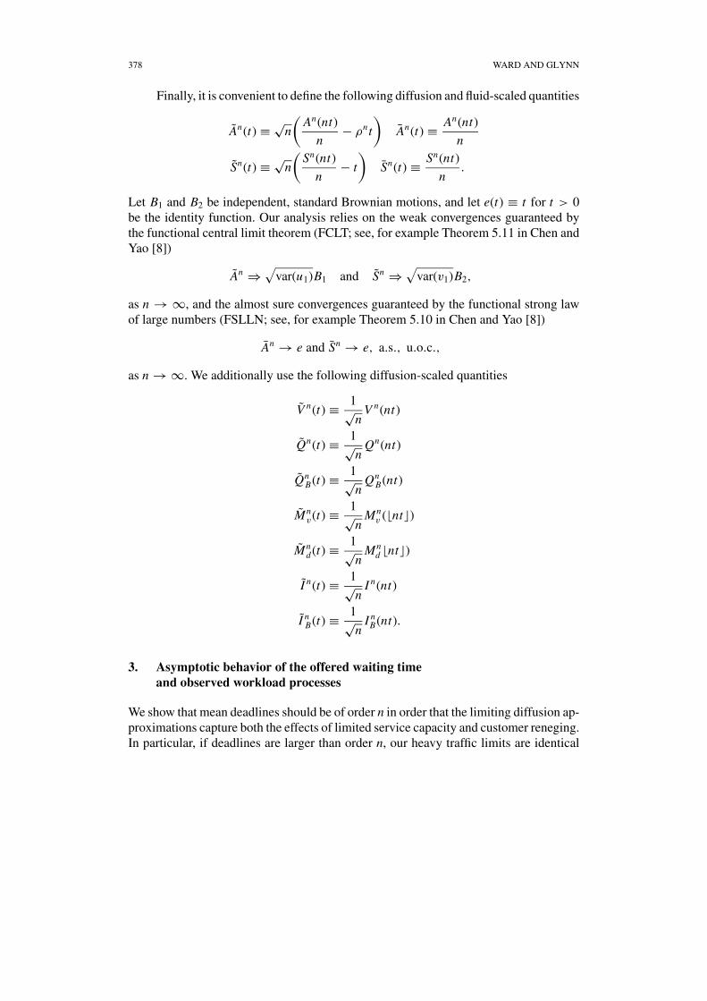
Finally, it is convenient to define the following diffusion and fluid-scaled quantities
An(t) ≡ √n
(An(nt)
n− ρnt
)An(t) ≡ An(nt)
n
Sn(t) ≡ √n
(Sn(nt)
n− t
)Sn(t) ≡ Sn(nt)
n.
Let B1 and B2 be independent, standard Brownian motions, and let e(t) ≡ t for t > 0be the identity function. Our analysis relies on the weak convergences guaranteed bythe functional central limit theorem (FCLT; see, for example Theorem 5.11 in Chen andYao [8])
An ⇒√
var(u1)B1 and Sn ⇒√
var(v1)B2,
as n → ∞, and the almost sure convergences guaranteed by the functional strong lawof large numbers (FSLLN; see, for example Theorem 5.10 in Chen and Yao [8])
An → e and Sn → e, a.s., u.o.c.,
as n → ∞. We additionally use the following diffusion-scaled quantities
V n(t) ≡ 1√n
V n(nt)
Qn(t) ≡ 1√n
Qn(nt)
QnB(t) ≡ 1√
nQn
B(nt)
Mnv(t) ≡ 1√
nMn
v ( nt�)
Mnd(t) ≡ 1√
nMn
d nt�)
I n(t) ≡ 1√n
I n(nt)
I nB(t) ≡ 1√
nI n
B(nt).
3. Asymptotic behavior of the offered waiting timeand observed workload processes
We show that mean deadlines should be of order n in order that the limiting diffusion ap-proximations capture both the effects of limited service capacity and customer reneging.In particular, if deadlines are larger than order n, our heavy traffic limits are identical
GI/GI/1 GI QUEUES 379
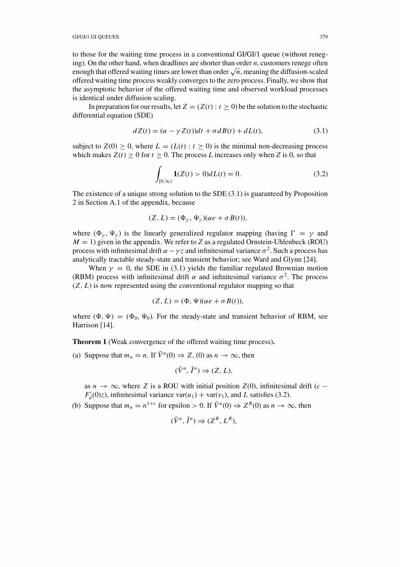
to those for the waiting time process in a conventional GI/GI/1 queue (without reneg-ing). On the other hand, when deadlines are shorter than order n, customers renege oftenenough that offered waiting times are lower than order
√n, meaning the diffusion-scaled
offered waiting time process weakly converges to the zero process. Finally, we show thatthe asymptotic behavior of the offered waiting time and observed workload processesis identical under diffusion scaling.
In preparation for our results, let Z = (Z (t) : t ≥ 0) be the solution to the stochasticdifferential equation (SDE)
d Z (t) = (α − γ Z (t))dt + σd B(t) + d L(t), (3.1)
subject to Z (0) ≥ 0, where L = (L(t) : t ≥ 0) is the minimal non-decreasing processwhich makes Z (t) ≥ 0 for t ≥ 0. The process L increases only when Z is 0, so that
∫
[0,∞)1(Z (t) > 0)d L(t) = 0. (3.2)
The existence of a unique strong solution to the SDE (3.1) is guaranteed by Proposition2 in Section A.1 of the appendix, because
(Z , L) = (γ , γ )(αe + σ B(t)),
where (γ , γ ) is the linearly generalized regulator mapping (having � = γ andM = 1) given in the appendix. We refer to Z as a regulated Ornstein-Uhlenbeck (ROU)process with infinitesimal drift α −γ z and infinitesimal variance σ 2. Such a process hasanalytically tractable steady-state and transient behavior; see Ward and Glynn [24].
When γ = 0, the SDE in (3.1) yields the familiar regulated Brownian motion(RBM) process with infinitesimal drift α and infinitesimal variance σ 2. The process(Z , L) is now represented using the conventional regulator mapping so that
(Z , L) = (, )(αe + σ B(t)),
where (, ) = (0, 0). For the steady-state and transient behavior of RBM, seeHarrison [14].
Theorem 1 (Weak convergence of the offered waiting time process).
(a) Suppose that mn = n. If V n(0) ⇒ Z , (0) as n → ∞, then
(V n, I n) ⇒ (Z , L),
as n → ∞, where Z is a ROU with initial position Z (0), infinitesimal drift (c −F ′
d(0)z), infinitesimal variance var(u1) + var(v1), and L satisfies (3.2).
(b) Suppose that mn = n1+ε for epsilon > 0. If V n(0) ⇒ Z R(0) as n → ∞, then
(V n, I n) ⇒ (Z R, L R),
380 WARD AND GLYNN
as n → ∞, where Z R is a RBM with infinitesimal drift c, infinitesimal variancevar(u1) + var(v1), and L R satisfies (3.2) with Z R substituted for Z .
(c) Suppose that mn = n1−ε for 1 > ε > 1/2. If V n(0) ⇒ 0 as n → ∞, then
V n ⇒ 0,
as n → ∞.
The proof of Theorem 1 uses the following two Lemmas, whose proofs can befound in Section A.2 of the appendix.
Lemma 1. For any t > 0, given ε > 0, there exists K such that for all n
P
(max
j=1,..., nt�1√n
V n(tn,−
j
)> K
)< ε.
Lemma 2. Suppose mn = n p for p > 1/2. Then
Mnd ⇒ 0
as n → ∞.
Proof of Theorem 1.
Part (a): From the pathwise equation for V in (2.5) and our assumption that mn = n,
V n(t) + F ′(0)∫ t
0V n(s)ds = X n(t) + I n(t),
where
X n(t) ≡ An(t) + Mnv( An(t)) + √
n(ρn − 1)t
− Mnd( An(t)) + F ′(0)
∫ t
0V n(s)ds −
∫ t
0
√nF(n−1/2V n(s))d An(s).
Since I n(0) = 0, I n is non-decreasing, I n increases only when V n = 0, and Proposition 2guarantees the uniqueness of the linearly generalized regulator mapping, for � ≡ F ′
d(0),
(V n, I n) = (�, �) (X n). (3.3)
Let B1, B2, and B be standard, independent Brownian motions. By the FCLT,
An ⇒√
var(u1)B1 (3.4)
GI/GI/1 GI QUEUES 381
as n → ∞. Next, observe that
Mnv(t) = 1√
n
nt�∑
j=1
(v j − 1) − 1√n
nt�∑
j=1
(v j − 1)1{
V(tn,−
j
) ≥ dnj
}. (3.5)
By Donsker’s theorem, the first term in (3.5) weakly converges to√
var(v1)B2. Therefore,to show
Mnv ⇒
√var(v1)B2,
it is sufficient to show the second term in (3.5) weakly converges to 0. Let δ > 0 andε > 0. By Lemma 1, we can choose K so that
P
(max
j=1,..., nt�n−1/2V n
(tn,−
j
)> K
)< δ/2. (3.6)
Also, for n large enough,
(18 × 2√
2)2 E |v1 − 1|2 nt�nε2
F
(K√
n
)<
δ
2, (3.7)
since F(n−1/2 K ) → 0 as n → ∞. Finally, the following chain of inequalities
P
(sup
0≤s≤tn−1/2
ns�∑
j=1
(v j − 1)1{
V(tn,−
j
) ≥ dnj
}> ε
)
≤ P
(sup0≤s≤t n−1/2 ∑[ns]
j=1(v j − 1)1{
V(tn,−
j
) ≥ dnj
}> ε
∩ max j=1,..., nt� n−1/2V n(tn,−
j
) ≤ K
)+ δ
2
≤ P
(sup
0≤s≤t
∣∣∣∣∣1√n
ns�∑
j=1
(v j − 1)1{dn
j ≤ √nK
}∣∣∣∣∣ > ε
)+ δ
2
≤ E∣∣ ∑ nt�
j=1(v j − 1)1{dn
j ≤ √nK
}∣∣2
nε2+ δ
2(Kolmogorov’s submartingale inequality)
≤ (18 × 2√
2)2E
∑ nt�j=1(v j − 1)21
{dn
j ≤ √nK
}
nε2+ δ
2(Burkholder’s inequality)
= (18 × 2√
2)2 E(v1 − 1)2 nt�nε2
F
(K√
n
)+ δ
2
≤ δ
2+ δ
2= δ
shows the second term in (3.5) weakly converges to 0. Therefore, Mnv ⇒ √
var(v1)B2
and, by the random time change theorem, since An → e as n → ∞ a.s., u.o.c. by the
382 WARD AND GLYNN
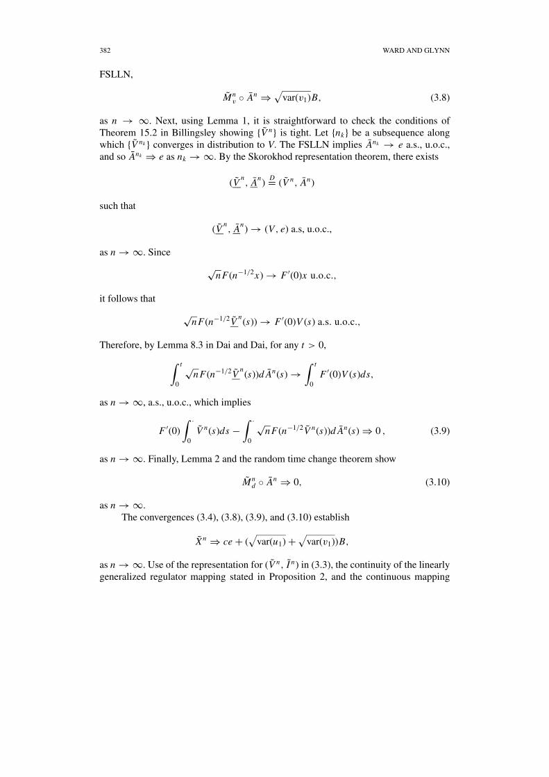
FSLLN,
Mnv ◦ An ⇒
√var(v1)B, (3.8)
as n → ∞. Next, using Lemma 1, it is straightforward to check the conditions ofTheorem 15.2 in Billingsley showing {V n} is tight. Let {nk} be a subsequence alongwhich {V nk } converges in distribution to V. The FSLLN implies Ank → e a.s., u.o.c.,and so Ank ⇒ e as nk → ∞. By the Skorokhod representation theorem, there exists
(Vn, An)
D= (V n, An)
such that
(Vn, An) → (V, e) a.s, u.o.c.,
as n → ∞. Since
√nF(n−1/2x) → F ′(0)x u.o.c.,
it follows that
√nF(n−1/2V
n(s)) → F ′(0)V (s) a.s. u.o.c.,
Therefore, by Lemma 8.3 in Dai and Dai, for any t > 0,
∫ t
0
√nF(n−1/2V
n(s))d An(s) →
∫ t
0F ′(0)V (s)ds,
as n → ∞, a.s., u.o.c., which implies
F ′(0)∫ ·
0V n(s)ds −
∫ ·
0
√nF(n−1/2V n(s))d An(s) ⇒ 0 , (3.9)
as n → ∞. Finally, Lemma 2 and the random time change theorem show
Mnd ◦ An ⇒ 0, (3.10)
as n → ∞.The convergences (3.4), (3.8), (3.9), and (3.10) establish
X n ⇒ ce + (√
var(u1) +√
var(v1))B,
as n → ∞. Use of the representation for (V n, I n) in (3.3), the continuity of the linearlygeneralized regulator mapping stated in Proposition 2, and the continuous mapping
GI/GI/1 GI QUEUES 383
theorem shows (recalling that � = F ′d(0))
(V n, I n) ⇒ (�, �) (ce + (√
var(u1) +√
var(v1))B),
a ROU with infinitesimal drift c − �z and infinitesimal variance var(u1) + var(v1).
Part (b): When mn = n1+ε , the pathwise equation for V in (3.3) can be written as
V n(t) = X n(t) + I n(t),
where
X n(t) ≡ An(t) + Mnv( An(t)) + √
n(ρn − 1)t − Mnd( An(t))
−∫ t
0
√nF(n−1/2−ε V n(s)) d An(s).
Similar to the proof of part (a), by the properties of I n and the uniqueness of theconventional regulator mapping,
(V n, I n) (, ) (X n). (3.11)
For any x ≥ 0,
√nF(n−1/2−εx) → 0,
as n → ∞, and so it is straightforward to use the tightness of V n established in Lemma 1to show
∫ ·
0
√nF(n−1/2−ε V n(s)) d An(s) ⇒ 0.
Identical arguments to those in part (a) show the weak convergences of An, Mnv ◦ An,
and Mnd ◦ An , and so
X n ⇒ ce + (√
var(u1) +√
var(v1))B,
as n → ∞. Therefore, from (3.11), the continuity of the conventional regulator mapping,and the continuous mapping theorem,
(V n, I n) ⇒ (, ) (ce + (√
var(u1) +√
var(v1))B),
a RBM with infinitesimal drift c and infinitesimal variance var(u1) + var(v1).
384 WARD AND GLYNN
Part (c): When mn = n1−ε , the pathwise equation for V in (2.5) can be written as
V n(t) = An(t) + Mnv( An(t)) + √
n(ρn − 1)t − Mnd( An(t))
−∫ t
0
√nF(n−1/2+ε V n(s))d An(s) + I n(t)
≥ 0.
Since, as in the proofs of parts (a) and (b), for B a standard Brownian motion,
An + Mnv ◦ An + √
n(ρn − 1)e − Mnd ◦ An ⇒ ce + (
√var(u1) +
√var(v1))B,
a proper random variable, I n only increases when V n = 0, and for any x ≥ 0,√
nF(n−1/2+εx) → +∞as n → ∞, arguments similar to those in Theorem 2 in Section 3.2 in Reiman [21] show
V n ⇒ 0
as n → ∞.
Our next theorem shows that customers who abandon the system without receivingservice do not influence queueing fluctuations too much. In particular, the limitingbehavior of the workload process is the same regardless of whether or not the workloadof customers who eventually renege is included.
Theorem 2 (Weak convergence of the observed workload process). Theorem 1 holdswith W n replacing V n , and the requirement that ε > 1/6 in part (c).
Proof. From Theorem 1 and the definition of W in (2.2), we must show that for anygiven t, ε, δ > 0, and for dn
i = n pwi with p > 5/6, for large enough n
P
(sup
0≤s≤t
1√n
An(ns)∑
i=1
vi 1{
V n(tn,−i
) ≥ dni and tn
i ≤ ns ≤ tni + dn
i
}> ε
)< δ.
Since the supremum in the above expression occurs at t and n−1 An → e a.s., u.o.c., bythe random time change theorem, it is enough to show, for large n,
P
(1√n
nt�∑
i=1
vi 1{
V n(tn,−i
) ≥ dni and tn
i ≤ nt ≤ tni + dn
i
}> ε
)< δ.
By Lemma 1, we can choose K large enough so that
P
(max
j=1,..., nt�1√n
V n(tn,−
j
)> K
)<
δ
2
GI/GI/1 GI QUEUES 385
for all n, and so
P
(1√n
nt�∑
i=1
vi 1{
V n(tn,−i
) ≥ dni and tn
i ≤ nt ≤ tni + dn
i
}> ε
)
≤ P
(1√n
nt�∑
i=1
vi 1{
V n(tn,−i
) ≥ dni and tn
i ≤ nt ≤ tni + dn
i
}
> ε ∩ maxi=1,..., nt�
1√n
V n(tn,−
j
) ≤ K
)+ δ
2
≤ P
(1√n
nt∑
i=ρnnt−n5/6
vi 1{n p−1/2wi ≤ K } >ε
2
)(3.12)
+ P
(1√n
ρnnt−n5/6∑
i=1
vi 1{nt − √
nK ≤ tni
}>
ε
2
)+ δ
2. (3.13)
To finish the proof, we show terms (3.12) and (3.13) are both less than or equal toδ/4. Since p > 5/6,
√n(ρn − 1) → c < ∞ as n → ∞, F ′
d(0) < ∞, and var(u1) < ∞,we can choose n large enough so that
2K
εn5/6−p(n1/6t(1 − ρn) + 1)
F(n1/2−p K )
n1/2−p K<
δ
4(3.14)
n−1/6 2(t − n−1/6)
ε
(ρnt − n−1/6)E(u1 − 1)2
(1 − n−1/3 Kρn)2<
δ
4. (3.15)
For term (3.12), by Markov’s inequality and (3.14)
(3.12) ≤ 2
ε√
nE
[nt∑
i=ρnnt−n5/6
vi 1{n p−1/2wi ≤ K }]
= 2
ε√
n(nt − ρnnt + n5/6)F(n1/2−p K )
= 2K
εn5/6−p(n1/6t(1 − ρn) + 1)
F(n1/2−p K )
n1/2−p K
<δ
4.
386 WARD AND GLYNN
For term (3.13), by two applications of Markov’s inequality and (3.15),
(3.13) ≤ 2
ε√
nE
[ρnnt−n5/6∑
i=1
vi 1{nt − √
nK ≤ tni
}>
ε
2
]
= 2
ε√
n
ρnnt−n5/6∑
i=1
P
(ρn(nt − √
nK ) ≤i∑
j=1
u j
)
≤ 2
ε√
n(ρnnt − n5/6)P
(ρn(nt − √
nK ) ≤ρnnt−n5/6∑
j=1
u j
)
= 2(ρnnt − n5/6)
ε√
nP
(n5/6 − √
nKρn ≤ρnnt−n5/6∑
j=1
(u j − 1)
)
≤ 2(ρnnt − n5/6)
ε√
n
E( ∑ρnnt−n5/6
j=1 (u j − 1))2
(n5/6 − √nKρn)2
= n−1/6 2(ρnt − n−1/6)
ε
(ρnt − n−1/6)E(u1 − 1)2
(1 − n−1/3 Kρn)2
<δ
4.
4. Asymptotic behavior of the reneging and balking queue-length processes
We first develop a heavy traffic limit theorem for the queue-length process in our renegingmodel that shows a state-space collapse. In particular, the limiting behavior of the queue-length process is close to the offered waiting time (and the observed workload processby use of Theorem 2). We next show that the behavior of the queue-length process inour balking model, in which customer processing times are not observable is identicalin heavy-traffic.
Theorem 3 (Weak convergence of the queue-length process for the reneging model).Theorem 1 holds with Qn replacing V n , and the requirement that ε > 1/6 in part (c).
Proof. We leverage off the weak convergence result for the offered waiting time processin Theorem 1. Our proof is similar to Theorem 4 in Reiman [21], which shows the weakconvergence of the diffusion-scaled queue-length process in a GI/GI/1 queue by usinga weak convergence result for the waiting time process. However, we must account forreneging customers.
Let an(t) be the arrival time of the customer in service at time t in the nth system.If the server is idle, let an(t) = t . Since the service discipline is FIFO, the number ofcustomers currently in queue is less than the number that have arrived after the customers
GI/GI/1 GI QUEUES 387
currently in service plus one, An(t) − An(an(t)) + 1. Additionally, the current queue-length exceeds An(t)− An(an(t)) minus the number of customers that have arrived afterthe one currently in service that will eventually renege, and so
An(t) − An(an(t)) −An(t)∑
i=An(an(t))
1{
V n(tn,−i
) ≥ dni
} ≤ Qn(t) ≤ An(t) − An(an(t)) + 1,
or
|Qn(t) − V n(t)| ≤ |An(t) − An(an(t)) − V n(t)| + 1 +An(t)∑
i=An(an(t))
1{
V n(tn,−i
) ≥ dni
}.
Time and space-scaling the above equation along with some algebra yields
|Qn(t) − V n(t)| ≤ | An(t) − ¯An(an(t))| + n−1/2 + |ρn(V n(an(t)−) − V n(t))|
+ |ρn(√
n(t − an(t)) − V n(an(t)−))| + |V n(t)(ρn − 1)|
+ n−1/2An(nt)∑
i=An(an(nt))
1{
V n(tn,−i
) ≥ dni
}, (4.1)
where an(t) = n−1a(nt).We now argue the right-hand side of (4.1) weakly converges to 0, which is sufficient
to complete the proof. For t ≥ 0 and n ≥ 1, since the server works at rate 1 and thesystem is FIFO,
V n(an(t)−) ≤ t − an(t) ≤ V n(an(t)−) + vAn(an(t)). (4.2)
From Lemma 3 in Iglehart and Whitt [15], for any t ≥ 0
as n → ∞. Since V n ⇒ Z as n → ∞ by Theorem 1 and an(s) ≤ s,
1√n
(V n ◦ an) ⇒ 0, (4.5)
as n → ∞. Together (4.4) and (4.5) imply
an ⇒ e, (4.6)
388 WARD AND GLYNN
as n → ∞. Since An and V n both weakly converge to a continuous limit process,
An − An ◦ an ⇒ 0 and V n − V n ◦ an ⇒ 0, (4.7)
as n → ∞. Since ρn → 1 as n → ∞ and for any t > 0, sup0≤s≤t V n(s) is tight byLemma 1,
V n(ρn − 1) ⇒ 0, (4.8)
as n → ∞. Therefore, by (4.1) and the convergences in (4.4), (4.7), and (4.8), tocomplete the proof, it is sufficient to show
n−1/2An(n·)∑
i=An(an(n·))1{
V n(tn,−i
)< dn
i
} ⇒ 0,
as n → ∞.Since
n−1/2An(nt)∑
i=An(an(nt))
1{
V n(tn,−i
)< dn
i
}
= n−1/2An(nt)∑
i=An(an(nt))
P(V n
(tn,−i
) ≥ dni
)
+ n−1/2An(n·)∑
i=An(an(n·))
(1{
V n(tn,−i
)< dn
i
} − E[1{
V n(tn,−i
) ≥ dni
}∣∣Fi−1])
and arguments similar to Lemma 2 show the second term in the right-hand side of theabove expression weakly converges to 0, to complete the proof, we must show
n−1/2An(n·)∑
i=An(an(n·))P
(V n
(tn,−i
) ≥ dni
) ⇒ 0,
as n → ∞. Given ε and δ, choose K large enough so that
P
(max
j=0,1,..., nt�n−1/2V n
(tn,−
j
)> K
)< δ/2. (4.9)
for all n. (Lemma 1 guarantees such a K exists.) Also, the FSLLN, the fact that p = 1implies n1/2 F(n1/2−p K ) → f (0)K and p > 1 implies n1/2 F(n1/2−p K ) → 0 as n →∞, and the convergence in (4.6) imply we can choose n large enough so that
P
(sup
0≤s≤t( An(s) − An(an(s)))n1/2 F(K n1/2−p) > ε
)< δ/2. (4.10)
GI/GI/1 GI QUEUES 389
From (4.9) and (4.10)
P
((sup
0≤s≤t
1√n
An(ns)∑
i=An(an(ns))
P(V n
(tn,−i
) ≥ dni
))
> ε
)
≤ P
(sup
0≤s≤t( An(s) − An(an(s))
)n1/2 F(K n1/2−p) > ε) + δ/2
< δ.
Part 3 follows as in the proof of Theorem 1 (c) because a little algebra shows
Qn(t) = An(t) − Sn(Bn(t)) + √nt(ρn − 1) − Mn
d( An(t)) + �n(t)
−∫ t
0
√nF
(n−1/2+ε V n(s)
)d An(s) + I n(t),
and√
nF(n−1/2+εx) → +∞ as n → ∞. (Note that we needed p > 5/6 to conclude,similar to the proof of Theorem 2, that �n ⇒ 0 as n → ∞.)
Our final theorem shows the diffusion-scaled queue-length process in our balkingmodel has the same limiting behavior as the observed queue-length process in ourreneging model.
Theorem 4 (Weak convergence of the queue-length process for the balking model).Theorem 1 holds with Qn
B replacing V n .
Proof. Define
MnB(i) ≡
i∑
j=1
1{
QnB
(tn,−i
) − 1 ≥ dni
} − E[1{
QnB
(tn,−i
) − 1 ≥ dni
} ∣∣Fi−1],
and observe that (1) MnB is a martingale and (2) E[1{Qn
B(t−i ) − 1 ≥ dn
i } |Fi−1] =Fn(Qn
B(tn,−i ) − 1). (Recall the definition of Fi at the end of Section 1.1.) Algebraic
manipulations of the pathwise equation for Q B in (2.4) show
QnB(t) +
∫ t
0
√nF
(Q B(ns) − 1
mn
)d An(s) = X n(t) + I n
B(t), (4.11)
where
X nB(t) ≡ An(t) − Sn
(Bn
B(t)) + √
nt(ρn − 1) − MnB( An(t)),
for BnB(t) ≡ n−1 Bn
B(nt), MnB(t) = n−1/2 Mn
B( nt�), and all other scaled quantities areas defined in Section 2.3. We can also write the pathwise equation for Q B in terms of
390 WARD AND GLYNN
the fluid-scaled quantities QnB(t) ≡ n−1 Qn
B(nt), An, Sn, BnB, and I n
B(t) ≡ n−1 I nB(nt) as
follows
QnB(t) = X n
B(t) + I nB(t), (4.12)
where
X nB(t) ≡ An(t) − ρnt − Sn
(Bn
B(t)) + Bn
B(t) + t(ρn − 1)
− n−1An(nt)∑
i=1
1{
Q B(tn,−i
) − 1 ≥ dni
}.
Since I nB and Qn
B satisfy conditions (C1) and (C2) in Section A.1 for � = 0, we canwrite (Qn
B, I nB) using the conventional regulator mapping
(Qn
B, I nB
) = (, )(X n
B
). (4.13)
By the FSLLN, the fact that BnB(t) ≤ t for all n, and the fact that ρn → 1 as
n → ∞, we can conclude
X nB ⇒ 0,
as n → ∞, provided we can show
1
n
An(n·)∑
i=1
1{
Q B(tn,−i
) − 1 ≥ dni
} ⇒ 0, (4.14)
as n → ∞. Let ε > 0, δ > 0, and t > 0. Similar arguments to those in Lemma 1 showthere exists a K such that for all n
P
(max
j=1,..., nt�n−1/2 Qn
B
(tn,−
j
)> K + 1
)<
δ
2. (4.15)
Also, for large enough n, since p ≥ 1/2,
F(K n1/2−p) <δε
2t. (4.16)
Recalling that dni = n pwi , Markov’s inequality, (4.15), and (4.16) show
P
(sup
0≤s≤t
∣∣∣∣∣ n−1ns∑
i=1
1{
Q B(tn,−t
) − 1 ≥ dni
}∣∣∣∣∣ > ε
)
= P
(n−1
nt∑
i=1
1{
QnB
(tn,−i
) − 1 ≥ dni
}> ε
)
GI/GI/1 GI QUEUES 391
≤ P
(1
n
nt∑
i=1
1{
QnB
(tn,−i
) − 1 ≥ dni
}> ε ∩ max
j=1,..., nt�1√n
QnB
(tn,−t
)> K
)+ δ
2
≤∑nt
i=1 E[1{dni ≤ √
nK }]nε
+ δ
2
= t
εF(n1/2−p K ) + δ
2= δ,
which shows (4.14) using the random time change theorem. Since X nB ⇒ 0 as n → ∞,
from (4.13),
(Qn
B, I nB
) ⇒ (0, 0),
as n → ∞, which implies
BnB → e, (4.17)
as n → ∞.By (4.17), the FCLT, the random time change theorem, and an argument similar
to Lemma 2 establishing MnB ⇒ 0,
X nB ⇒ ce +
√var(u1) + var(v1)B
as n → ∞, where B is a standard Brownian motion. Similar arguments to those in theproof of Theorem 1 establish the asymptotic behavior of the integral term
∫ t
0
√nF
(Q B(ns) − 1
mn
)d An(s),
and complete the proof.
5. Proposed approximations and simulation results
Our weak convergence results in Theorems 3 and 4 suggest approximating the queue-length process in either our balking or reneging model with a ROU process. Specifically,consider a system having arrival rate ρ, mean service time 1, and deadline distributionfunction F. We propose to approximate the queue-length process with the ROU Z havinginfinitesimal drift ρ − 1 − F ′(0)z, infinitesimal variance ρvar(u1) + (ρ ∧ 1)var(v1), andsteady-state mean (as given in Proposition 18.3 in Browne and Whitt [6])
Z = E[N
(mρ, b2
ρ
) ∣∣ 0 ≤ N(mρ, b2
ρ
)],
392 WARD AND GLYNN
where N (m, b2) is a normal random variable with mean m and variance b2, and
mρ = ρ − 1
F ′(0)and b2
ρ = ρvar(u1) + (ρ ∧ 1)var(v1)
2F ′(0).
To understand the intuition behind the proposed approximation, first rewrite thequeue-length process evolution equation (2.3) as
For any x ∈ , as n → ∞, nF(n−1x) → F ′(0)x and An → e a.s., u.o.c. When m ≡ nis large (meaning the system has traffic intensity ρ close to 1 and mean deadlines oforder (1 − ρ)−2), for each t > 0, Theorem 3 and the preceding observation suggest
∫ t
0F
(V n(s)
n
)d An(s) =
∫ t
0nF(n−1V n(s))d An(s)
D≈∫ t
0nF(n−1 Qn(s))d An(s)
D≈∫ t
0F ′(0)Qn(s)ds,
where the symbolD≈ denotes approximately equal in distribution. Hence when ρ is close
to 1 and mean deadlines are of order (1 − ρ)−2, for � = F ′(0),
(Q, I )D≈ (�, �) (X ). (5.1)
The FCLT shows for t > 0
A(t) − ρtD≈ √
nB1
(t
n
)D= B1(t)
S(t) − tD≈ B2(t),
where B1 and B2 are two independent zero-mean Brownian motions with infinitesimalvariances ρvar(u1) and var(v1) respectively. The assumption that the cumulative busy
GI/GI/1 GI QUEUES 393
time in [0, t], B(t) is proportional to (ρ ∧ 1)t implies for t > 0
S(B(t)) − B(t)D≈ B2 ((ρ ∧ 1)t).
Therefore, because Lemma 2 and a slight modification of the proof of Theorem 2 shown−1/2εn(·n) ⇒ 0 as n → ∞, the process X can be approximated by a Brownian motionW with drift ρ −1 and variance ρvar(u1)+ (ρ ∧1)var(v1). The representation (5.1) thenestablishes
(Q, I )D≈ (�, �) (W ),
a ROU satisfying the stochastic equation (3.1) with α = ρ−1 and σ 2 = ρvar(u1)+(ρ∧1)var(v1). Observe that when � = 0 (meaning the effects of reneging/balking are notaccounted for in the limiting diffusion), our proposed approximation is a RBM R withinfinitesimal drift ρ − 1, infinitesimal variance ρvar(u1) + (ρ ∧ 1)var(v1), and steadystate mean (for ρ < 1)
R = ρ(var(u1) + var(v1))
2(1 − ρ),
the standard heavy traffic approximation for a conventional GI/GI/1 queue when theprimitive inter-arrival and service time sequences {ui : i ≥ 0} and {vi : i ≥ 0} havemean 1; see Section 6.5 in Chen and Yao [8].
Of course, our proposal to approximate the steady-state mean queue-length withthe ROU steady state mean Z assumes the limit interchange
limt→∞ lim
n→∞ Qn(t)(?)= lim
n→∞ limt→∞ Qn(t)
is valid. Proposition 1 in Ward and Glynn verifies the interchange in a purely exponentialsetting. In general, we conjecture an argument similar to that in Gamarnik and Zeevi[11] verifies the interchange.
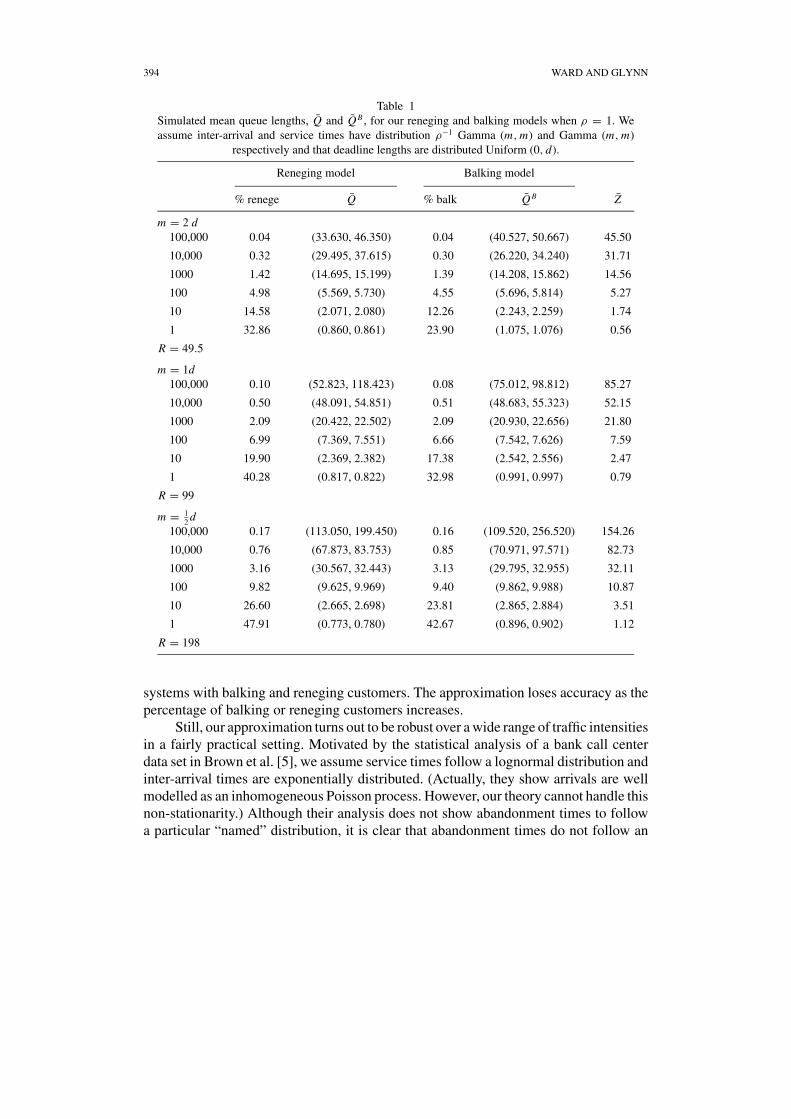
We compare the steady-state of the regulated O-U process Z with the steady-statemean queue-length that results from simulating our reneging and balking models. Forthe simulation results displayed in Tables 1 and 2, we present 95% confidence intervalsfor the mean queue-length found after 5 simulation runs (performed using the Extendsimulation language [1]), each of 500,000 time units. We also present the percent ofreneging and balking customers for both models, averaged over the 5 runs. As onewould expect, the percent of reneging customers is consistently slightly higher than thepercent of balking customers, and so the mean queue-length for the balking queue isgenerally slightly higher than that for the reneging queue with the same parameters.Although this is too fine a difference to evidence itself in our diffusion limits, it makessense to keep this in mind when applying our approximations.
Table 1 shows that under various assumptions on the variability of inter-arrival andservice times, our approximation predicts mean queue-lengths reasonably accurately in
394 WARD AND GLYNN
Table 1Simulated mean queue lengths, Q and Q B , for our reneging and balking models when ρ = 1. Weassume inter-arrival and service times have distribution ρ−1 Gamma (m, m) and Gamma (m, m)
respectively and that deadline lengths are distributed Uniform (0, d).
systems with balking and reneging customers. The approximation loses accuracy as thepercentage of balking or reneging customers increases.
Still, our approximation turns out to be robust over a wide range of traffic intensitiesin a fairly practical setting. Motivated by the statistical analysis of a bank call centerdata set in Brown et al. [5], we assume service times follow a lognormal distribution andinter-arrival times are exponentially distributed. (Actually, they show arrivals are wellmodelled as an inhomogeneous Poisson process. However, our theory cannot handle thisnon-stationarity.) Although their analysis does not show abandonment times to followa particular “named” distribution, it is clear that abandonment times do not follow an
GI/GI/1 GI QUEUES 395
Table 2Simulated mean queue lengths, Q and Q B , for our reneging and balking models. We assumeinter-arrival and service times have distribution ρ−1 Exponential (1) and Lognormal (1, 1)
respectively and that deadline lengths are distributed Uniform (0, 1000).
exponential distribution. We assume deadline times follow a uniform distribution. Table2 shows that our approximation is accurate across traffic intensities ranging between 0.5and 1—much lower than one might guess from our supporting limit theorems.
In many real-world service industry applications of queueing theory (such as callcenters, fast food restaurants, etc.), reneging and/or balking is present. If reneging and/orbalking percentages are small, one might be tempted to model the system as a conven-tional GI/GI/1 queue. In such settings, the appropriate diffusion approximation to thequeue is the RBM R defined a couple paragraphs earlier. Therefore, we take this oppor-tunity to present the mean steady-state queue-length predicted by the RBM R.
It is striking to observe the degree to which small percentages of reneging andbalking customers affect queue-lengths. For most all parameter combinations presentedin Tables 1 and 2, the RBM approximation does not provide reasonable predictions.It is only when d = 100, 000 in Table 1, and when ρ ≤ 0.8 in Table 2 that theRBM approximation is reasonably accurate. This seems to confirm a heuristic that canbe inferred from Theorems 1–4; that when deadline lengths are generally larger than(1 − ρ)−2, the presence of balking or reneging may be effectively ignored. Of course,the safe approach is to always model balking and reneging behavior since this heuristicmay be hard to confirm in practical situations.
A. Appendix
A.1. A regulator mapping with state dependence
For the reader’s convenience, we reproduce results on the existence, uniqueness, andcontinuity of a linearly generalized regulator mapping. For d a positive integer, x ∈D([0, ∞), d) having x(0) ≥ 0, and �, M square matrices of dimension d × d, the
396 WARD AND GLYNN
linearly generalized regulator mapping
(�, �)(x) : D([0, ∞), d) → D([0, ∞), [0, ∞)2d)
is defined by
(�, �)(x) ≡ (z, l),
where
(C1) z(t) + ∫ t0 �z(s)ds = x(t) + Ml(t) ≥ 0 for all t ≥ 0
(C2) l(0) = 0, l is non-decreasing, and∫ ∞
0 z j (t)dl j (t) = 0, j = 1, . . . , J .
Observe that if � is the zero matrix, we have the conventional regulator mapping dis-cussed in Section 7.2 of Chen and Yao [8]. We write , , where = 0 and = 0
to emphasize when we are referring to the conventional regulator mapping.The key to establishing the existence, uniqueness, and Lipschitz continuity of �
and � is understanding the properties of the following integral equation
u(t) = x(t) −∫ t
0�(u)(s)ds. (A.1)
In particular, as in Chen [7], define the mapping M : D([0, ∞), d) → D([0, ∞), d)(which exists uniquely by Lemma 3) by M(x) ≡ u, and observe that conditions (C1)–(C2) are satisfied when
(�, �)(x) = (, )(M(x)). (A.2)
The following Lemma, whose proof can be found in Reed and Ward [20], estab-lishes the basic properties of integral equations having the form (A.1).
Lemma 3. Suppose η : D([0, ∞),Rd) → D([0, ∞),Rd) is Lipschitz continuous.Then for any given x ∈ D([0, ∞),Rd), there exists a unique u ∈ D([0, ∞),Rd) thatsatisfies the integral equation
u(t) = x(t) −∫ t
0n(u)(s)ds, (A.3)
and has initial condition u(0) = x(0). Furthermore, the mappingMη : D([0, ∞),Rd) →D([0, ∞),Rd) defined by Mη(x) ≡ u is Lipschitz continuous.
Using the representation (A.2), Lemma 3, and Theorem 7.2 of Chen and Yao [8],which establishes the existence, uniqueness, and Lipschitz continuity of the mapping(, ), it is immediate to prove the following proposition.
GI/GI/1 GI QUEUES 397
Proposition 2. Suppose M has positive diagonal elements, non-positive off-diagonalelements, and a non-negative inverse. Then, for each x ∈ D([0, ∞), d) having x(0) ≥0, there exists a unique (z, l) satisfying (C1)–(C2). Furthermore, the mappings � and� are Lipschitz continuous.
A.2. Lemma proofs
Proof of Lemma 1. First observe that
P
(max
j=1,..., nt�1√n
V n(tn,−
j
)> K
)≤ P
(sup
0≤s≤t
1√n
V n
((ns)
∑ ns�i=1 ui
ns�)
> K
).
Since the strong law of large numbers establishes for any 0 < s ≤ t∑ ns�
i=1 ui
ns� → 1 a.s.,
by the random time change theorem, for a given ε > 0, it is enough to show there existsK such that
P
(sup
0≤s≤tV n(s) > K
)< ε. (A.4)
Define
R(t) ≡A(t)∑
i=1
vi − B(t).
The process R is the workload process in a conventional GI/GI/1 queue (without reneg-ing), for which the following convergence is known (see, for example, Theorem 1 inSection 3.2 in Reiman [21])
Rn ⇒ Z R, (A.5)
as n → ∞, where Rn(t) = n−1/2 Rn(nt), and Z R is a RBM with infinitesimal drift cand infinitesimal variance var(u1) + var(v1) (as in part (b) of Theorem 1). The weakconvergence in (A.5) implies there exists K such that for all n
P
(sup
0≤s≤tRn(s) > K
)< ε,
which implies (A.4) since R(t) ≥ V (t) for all t ≥ 0.
Proof of Lemma 2. For any given t, ε, δ > 0, we must show
P
(sup
0≤s≤t
∣∣Mnd (s)
∣∣ > ε
)= P
(max
i=1,..., nt�∣∣Mn
d (i)∣∣ > ε
√n
)< δ, (A.6)
398 WARD AND GLYNN
for large enough n. By a generalization of Kolmogorov’s inequality, and by Burkholder’sinequality (see, for example, Corollary 2.1 and Theorem 2.10 in Hall and Heyde [13]),
P
(max
i=1,..., nt�∣∣Mn
d (i)∣∣ > ε
√n
)
≤ E∣∣Mn
d ( nt�)∣∣2
nε2
≤ c
nε2E
[ nt�∑
j=1
(1{
V n(tn,−
j
) ≥ dnj
} − E[1{
V n(tn,−
j
) ≥ dnj
} ∣∣F j−1])2
],
where c is a finite constant-that does not depend on n.Since
(1{
V n(tn,−
j
) ≥ dnj
} − E[1{
V n(tn,−
j
) ≥ dnj
} ∣∣F j−1])2
≤ 1{
V n(tn,−
j
) ≥ dnj
} + E[1{
V n(tn,−
j
) ≥ dnj
} ∣∣F j−1]
and
E[1{
V n(tn,−
j
) ≥ dnj
} + E[1{
V n(tn,−
j
) ≥ dnj
} ∣∣F j−1]] = 2P
(V n
(tn,−
j
) ≥ dnj
),
the inequality
P
(max
i=1,..., nt�∣∣Mn
d (i)∣∣ > ε
√n
)≤ 2c
nε2
nt�∑
j=1
P(V n
(tn,−
j
) ≥ dnj
)(A.7)
holds.By Lemma 1, we can choose K large enough so that for all n
P
(max
j=1,..., nt�1√n
V n(tn,−
j
)> K
)<
δε2
4ct.
Since F is the distribution function of a positive random variable and p > 1/2, we canchoose n large enough so that
F(K n1/2−p) <δε2
4ct.
Therefore, for each j = 1, . . . , nt�,
P(V n
(tn,−
j
) ≥ dnj
) = P
(1√n
V n(t−j ) ≥ n p−1/2w j
)
≤ P(n p−1/2w j ≤ K ) + δε2
4ct
≤ δε2
2ct,
GI/GI/1 GI QUEUES 399
and so, from (A.7)
P
(max
i=1,..., nt�∣∣Mn
d (i)∣∣ > ε
√n
)≤ c2
nε2 nt�δε2
2ct= δ,
as required to complete the proof.
Acknowledgments
We would like to thank Hong Chen, Tom Kurtz and Shane Henderson for helpful dis-cussions relating to the issues discussed in this paper. We would also like to thank DaveKrahl for help with building our simulation models.
References
[1] : 2000, Extend: Professional simulation tools. Imagine That, 6830 Via Del Oro, Suite 230, San Jose,CA 95119, version 5 edition.
[2] : 2002, Cisco: Behind the hype. Business Week.[3] C.J. Ancker and A.V. Gafarian, Queueing with impatient customers who leave at random, Journal of
Industrial Engineering 13 (1962) 84–90.[4] F. Baccelli, P. Boyer and G. Hebuterne, Single-server queues with impatient customers, Adv. Appl.
Prob. 16 (1984) 887–905.[5] L. Brown, N. Gans, A. Mandelbaum, A. Sakov, H. Shen, S. Zeltyn and L. Zhao, Statistical analysis
of a telephone call center: A queueing-science perspective, Working Paper, (2002).[6] S. Browne and W. Whitt, Piecewise-linear diffusion processes, in: Advances in Queueing: Theory,
Methods, and Open Problems, ed. J. Dshalalow (CRC Press, 1995) pp. 463–480.[7] H. Chen, Generalized regulated mapping: Fluid and diffusion limits, Notes prepared for Avi Mandel-
baum, 1990.[8] H. Chen, and D.D. Yao, Fundamentals of Queueing Networks: Performance, Asymptotics, and Opti-
mization (Springer-Verlag, New York, 2001).[9] E. Coffman, A. Puhalskii, M. Reiman and P. Wright, Processor-shared buffers with reneging, Perfor-
mance Evaluation 19 (1994) 25–46.[10] B. Doytchinov, J. Lehoczky and S. Shreve, Real-time queues in heavy traffic with earliest-deadline-first
queue discipline, Annals of Applied Probability 11 (2001) 332–378.[11] D. Gamarnik and A. Zeevi, Validity of heavy traffic steady-state approximations in open queueing
networks, Working Paper, 2004.[12] O. Garnett, A. Mandelbaum and M. Reiman, Designing a call center with impatient customers,
Manufacturing and Service Operations Management 4 (2002) 208–227.[13] P. Hall and C.C. Heyde, Martingale Limit Theory and its Application (Academic Press, Inc., Boston,
1980).[14] J.M. Harrison, Brownian Motion and Stochastic Flow Systems (John Wiley & Sons, New York, 1985).[15] D.L. Iglehart and W. Whitt, Multiple channel queues in heavy traffic, I and II, Adv. Appl. Prob. 2
(1970) 150–177 and 355–364.[16] R. Lillo and M. Martin, Stability in queues with impatient customers, Stochastic Models 17 (2001).[17] A. Mandelbaum and S. Zeltyn, The impact of customers’ patience on delay and abandonment: Some
empirically-driven experiments with the M/M/N + G queue, OR Spectrum 26(3) (2004) 377–411.Special Issue on Call Centers.
400 WARD AND GLYNN
[18] C. Palm, Etude des delais d’attente, Ericson Technics 5 (1937) 37–56.[19] E.L. Plambeck, S. Kumar and J.M. Harrison, A multiclass queue in heavy traffic with throughput time
constraints: Asymptotically optimal dynamic controls, Queueing Systems 39 (2001) 23–54.[20] J. Reed and A.R. Ward, A diffusion approximation for a generalized Jackson network with reneging,
in: Proceedings of the 42nd Annual Allerton Conference on Communication, Control, and Computing,2004.
[21] M.I. Reiman, Some diffusion approximations with state space collapse, in: Lecture Notes in Controland Information Sciences, eds. F. Baccelli and G. Fayolle (Springer, 1984) vol. 60 pp. 209–240.
[22] R.E. Stanford, Reneging phenomena in single channel queues, Mathematics of Operations Research4 (1979) 162–178.
[23] A.R. Ward and P.W. Glynn, A diffusion approximation for a Markovian queue with reneging, QueueingSystems 43 (2003a) 103–128.
[24] A.R. Ward and P.W. Glynn, Properties of the reflected ornstein-uhlenbeck process, Queueing Systems44 (2003b) 109–123.
[25] W. Whitt, Improving service by informing customers about anticipated delays, Management Science45(2) (1999) 192–207.