Full Terms & Conditions of access and use can be found at http://www .tandfonline.com/action/journalIn formation?journalC ode=tprs20 Download by: [IIT Indian Institute of Technology - Mumbai] Date: 29 September 2015, At: 22:22 International Journal of Productio n Research ISSN: 0020-7543 (Print) 1366-588X (Online) Journal homepage: http://www.tandfonline.com/loi/tprs20 A discrete transfer function model to determine the dynamic stability of a vendor managed inventory supply chain S. M. Disney & D. R. Towill T o cite this article: S. M. Disney & D. R. Towill (2002) A discrete transfer function model to determine the dynamic stability of a vendor managed inventory supply chain, International Journal of Productio n Research, 40:1 , 179-204, DO I: 10.1080/0020754 0110072975 T o link to this article: http://dx.doi.org/10.1080/00207540110072975 Published online: 14 Nov 2010. Submit your article to this journal Article views: 414 View related articles Citing articles: 99 View citing articles
A discrete transfer function model to determinethe dynamic stability of a vendor managedinventory supply chain
S. M. Disney & D. R. Towill
To cite this article: S. M. Disney & D. R. Towill (2002) A discrete transfer function model to
determine the dynamic stability of a vendor managed inventory supply chain, International Journal of Production Research, 40:1, 179-204, DOI: 10.1080/00207540110072975
To link to this article: http://dx.doi.org/10.1080/00207540110072975
X …z† system z-transform transfer function multiplied by the
input z-transform transfer function,
Z z-transform operator.
VMI-APIOBPCS terms
AINV Actual INVentory,¬ 1=…1 ‡ Ta†,
AVCON average virtual consumption,
1=…1 ‡ Tq†,
COMRATE completion rate,
CONS consumption or market demand,
DES dispatches,
DINV distributors inventory holding,
dSS incremental change in the re-order point, R,
DWIP Desired Work In Progress,EINV Error in Inventory Holding,
EWIP Error in Work In Progress,
FINV factory inventory,
G gain (distributors re-order point/average consumption),
GIT Goods In Transit,
O order-up-to-point,
ORATE production order rate,
R re-order point,T transport quantity,
Ta consumption averaging time constant,
T · p p estimate of the production lead-time,
Ti inverse of inventory based production control law gain,
TINV target system inventory holding,
Tp the production lead-time in units of sampling intervals,
Tq exponential smoothing constant used at the distributor to
set R,
Tw inverse of WIP based production control law gain,VCON virtual consumption,
WIP Work In Progress.
2. Introduction
This paper is concerned with the analysis of a Vendor Managed Inventory (VMI)
supply chain. We focus on a one supplier, one customer relationship where the
demand levels are deemed to change signi®cantly over time, paying particular atten-
tion to the manufacturer’s production scheduling activities. A VMI system is aproduction and inventory control strategy where stock positions are known through-
out the supply chain for the purposes of setting production and distribution targets.
The z-transform is used to investigate the performance of the VMI system when
coupled with the APIOBPCS (Automatic Pipeline, Inventory and Order Based
Production Control System) production scheduling system (John et al . 1994). This
paper may be regarded as generalizing the approach of Popplewell and Bonney
(1987) and extending it to a two-echelon VMI supply chain. An important distinc-
tion here is the identi®cation (and hence avoidance) of instability in the supply chain.
The VMI scenario is ®rst described, followed by a description of previous work in
the ®eld. A formal description of the VMI system is then presented using causal loop
diagrams, block diagrams and z-transform transfer functions. Important managerial
insights are gained by inspecting the transfer functions. Furthermore, the stability
boundary is established via a novel technique based on the Tustin transformation
(Houpis and Lamont 1985). This boundary is determined as a relationship between
the two important system parameters of pipeline gain and inventory gain. The results
are con®rmed via the simulation of sample stable; critically stable; and unstable
supply chains. Hence, this paper not only con®rms the existence of the instability
problem but also provides guidance on parameter selection to guarantee a stable
response.
3. The VMI concept
VMI is a unique supply chain control strategy as advocated by Christopher
(1992), Holmstro È m, (1998) and Waller et al . (1999). VMI was however, describedin a presentation of a conceptual design of a production control system as far back as
Magee (1958). Magee also obviously regarded z-transforms as a powerful tool, as he
took responsibility for publishing the ®rst work (but sadly un®nished) on production
and inventory control to exploit them by Vassian (1954). The most signi®cant fact
about a VMI supply chain is that customers (we term the customer echelon in the
VMI supply chain as the distributor and the supplier echelon in the VMI supply
chain as the manufacturer for clarity) share inventory information and/or point of
sales data rather than orders with their suppliers. Alternatively, end sales data could
be determined from the net change in inventory levels if the distributor does notdisclose this information via EPOS. In addition, the manufacturer could net-o the
inventory from deliveries and sales if the distributor does not have the ability or
inclination to share inventory informatio n but can share end sales data. This is
usually done electronically. What matters in VMI is the allocation of responsibility
for decision-making and the agreed target setting.
The actual inventory at the distributor is then compared with a re-order point
that has been negotiated between the two parties. This is set to ensure adequate
Customer Service Levels (CSLs), without building up excessive stocks and can be
done via the standard re-order point model, for example see Wilkinson (1996). It
triggers a replenishment order that is delivered to the distributor based on the actual
end consumer sales. The replenishment order is calculated by subtracting the re-
order point from an order-up-to-point . Each party also agrees the order-up-to-
point. Payment is often triggered at this point and funds transferred electronically.
Sometimes payment is only triggered when the end consumer actually buys the
product from the shelf. Either party can do the forecasting of future demand. The
distributors’ stock requirements are updated regularly and based on the forecast to
ensure high CSL and good stock turns. The distributor replenishes this stock.The manufacturer then has to set the production targets. We have elected to do
this using the APIOBPCS structure as analysed in depth by John et al . (1994). It can
be expressed in words as, `Let the production targets be equal to the sum of an
exponentially smoothed (over Ta time units) representation of his perceived demand
(that is actually a sum of the stock adjustments at the distributor and the actual
sales), plus a fraction (1=Ti ) of the inventory error in stock, plus a fraction (1=Tw) of
the WIP error’. This is a generalization of the Popplewell and Bonney (1987) algor-
ithm and an extension to Sterman’s (1989) anchoring and adjustment heuristic as
identi®ed by Naim and Towill (1995) and further exploited by Mason-Jones et al .
(1997). By suitably adjusting parameters, APIOBPCS can be made to mimic a wide
range of industrial ordering scenarios including make-to-stock and make-to-order.
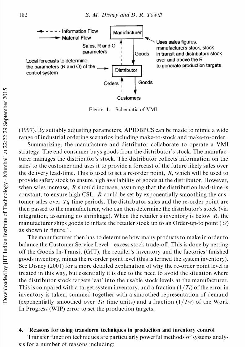
Summarizing, the manufacture and distributor collaborate to operate a VMI
strategy. The end consumer buys goods from the distributor’s stock. The manufac-
turer manages the distributor’s stock. The distributor collects information on the
sales to the customer and uses it to provide a forecast of the future likely sales over
the delivery lead-time. This is used to set a re-order point, R, which will be used to
provide safety stock to ensure high availability of goods at the distributor. However,when sales increase, R should increase, assuming that the distribution lead-time is
constant, to ensure high CSL. R could be set by exponentially smoothing the cus-
tomer sales over Tq time periods. The distributor sales and the re-order point are
then passed to the manufacturer, who can then determine the distributor’s stock (via
integration, assuming no shrinkage). When the retailer’s inventory is below R, the
manufacturer ships goods to in¯ate the retailer stock up to an Order-up-to point ( O)
as shown in ®gure 1.
The manufacturer then has to determine how many products to make in order to
balance the Customer Service Level ± excess stock trade-o. This is done by nettingo the Goods In-Transit (GIT), the retailer’s inventory and the factories’ ®nished
goods inventory, minus the re-order point level (this is termed the system inventory).
See Disney (2001) for a more detailed explanation of why the re-order point level is
treated in this way, but essentially it is due to the need to avoid the situation where
the distributor stock targets `eat’ into the usable stock levels at the manufacturer.
This is compared with a target system inventory, and a fraction (1=Ti ) of the error in
inventory is taken, summed together with a smoothed representation of demand
(exponentially smoothed over Ta time units) and a fraction (1=Tw) of the WorkIn Progress (WIP) error to set the production targets.
4. Reasons for using transform techniques in production and inventory control
Transfer function techniques are particularly powerful methods of systems analy-
sis for a number of reasons including:
. the use of standard forms, which simpli®es benchmarking and promulgation of
of a cash ¯ow, via a shortcut identi®ed in the Laplace domain, and was extended to
the discrete domain by GrubbstroÈ m (1991). The shortcut relies on the fact that the
NPV represented in exponential form has exactly the same structure as the Laplace
transform. Amazingly, the NPV of a cash ¯ow is calculated from the cash ¯ows’
transfer function by simply replacing the complex Laplace variable s with the con-
tinuous interest rate r or, in discrete time, replacing z with 1+the discrete interest
rate, r. In work of direct relevance to this paper Wikner (1994a) has exploited the
NPV transform on an IOBPCS (Towill 1982) model in continuous time. Yinzhong
and Grubbstro È m (1994) consider the application of the z-transform to net present
value problems. In later research at Linko È ping, Grubbstro È m and Wang (2000) have
investigated dierent types of capacity constraints using Input±Output Analysis and
the Laplace transform and Tang (2000) has been investigating the use of Laplace and
z-transforms in production and inventory control and using z-transforms of stoch-
astic demands and lead-times within MRP systems. Grubbstro È m and Tang (2000)highlight how the NPV transform can be used as an evaluation function for the
®nancial implementations of rescheduling.
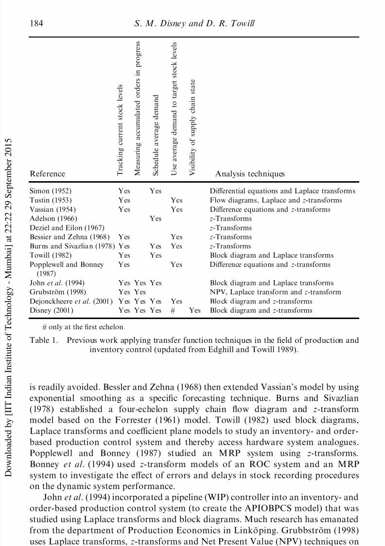
Finally, Dejonckheere et al . (2001) have been using z-transforms to investigate
the Bullwhip performance of common forecasting mechanisms such as moving
averages, exponential smoothing and demand signalling within Order-Up-To
models. Dejonckheere et al . (2000) used z-transforms and Fourier transforms to
design particular ordering decisions to suit particular demand patterns via the
Fourier plot and an optimization procedure to `match’ the frequency response to
the Fourier plot. This may be regarded as supply chain design via the `explicit ®lter’approach following the analytical results by Towill and del Vecchio (1994) and the
conceptual discussion by Towill et al . (2001). Table 1 brie¯y summarizes the histor-
ical development.
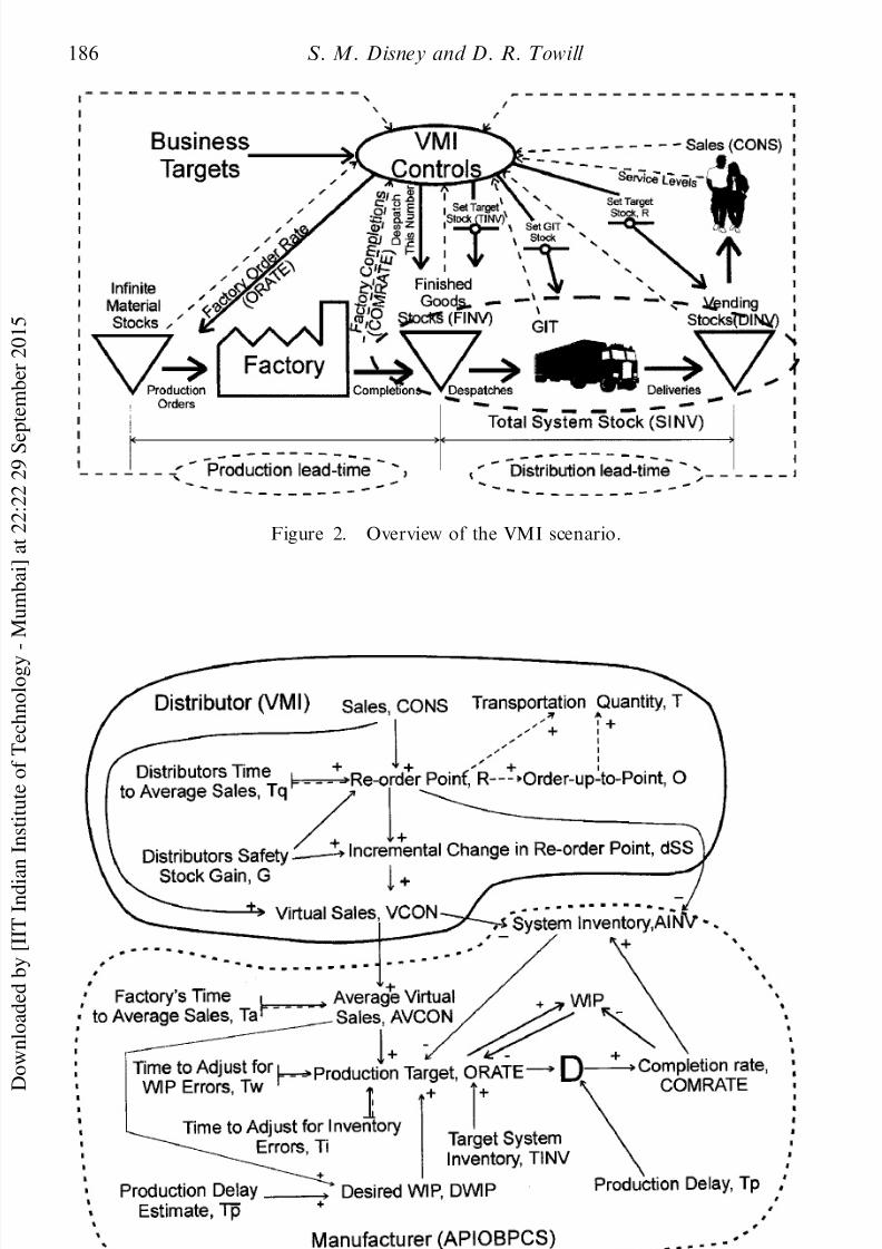
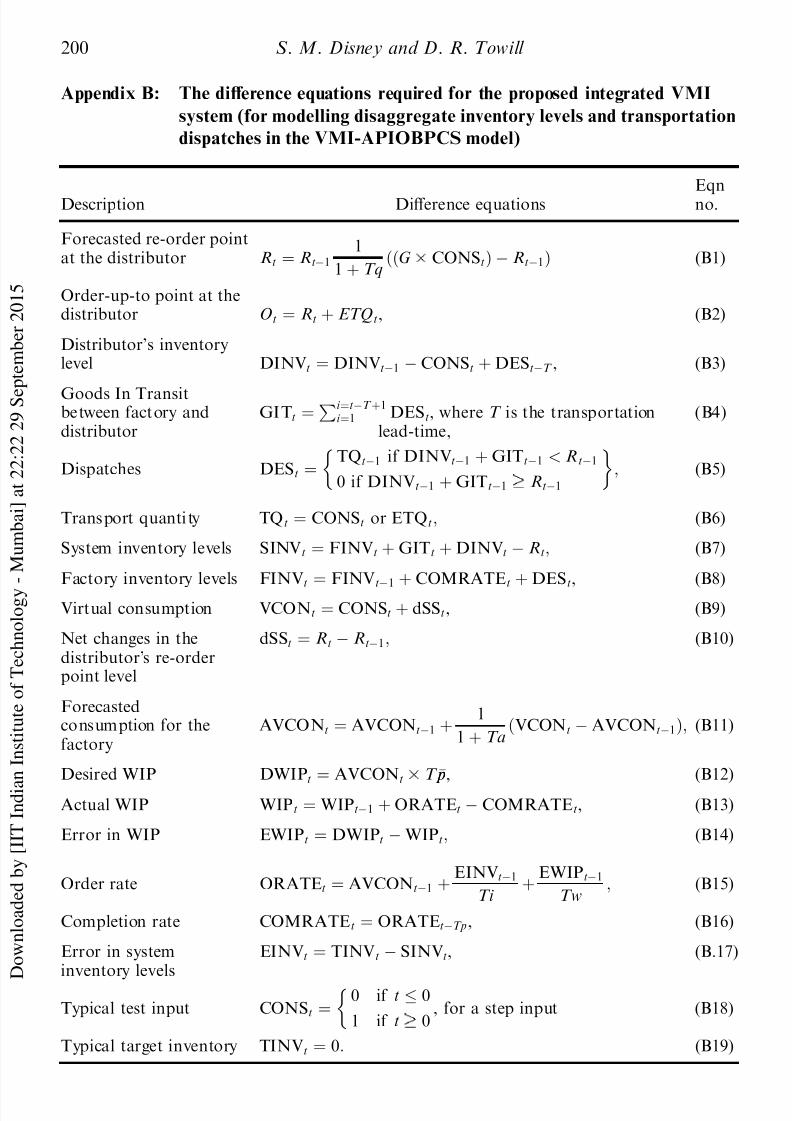
5. Formal description of VMI as an integrated system
Recall that the APIOBPCS structure can be expressed in words as, `Let the
production targets be equal to the sum of an exponentially smoothed representation
of demand (exponentially smoothed over Ta time units), plus a fraction (1=Ti ) of the
inventory error in stock, plus a fraction (1=Tw) of the WIP error’. In a multi-echelon
inventory decision-making environment, the inventory error corresponds to the
desired inventory in the factory minus the actual inventory in the factory.
However, to extend the APIOBPCS model into VMI-APIOBPCS, the manufac-
turer’s ®nished goods now encapsulate the distributor’s inventory, the manufac-
turer’s ®nished goods as well as the stock in transport minus the re-order point.
De®ning the net sum of these three stocks as the system stock, the VMI-APIOBPCS
can be expressed in words as, `Let the production targets be equal to the sum of anexponentially smoothed representation of demand (exponentially smoothed over Ta
time units), plus a fraction (1=Ti ) of the inventory error in system stock, plus a
fraction (1=Tw) of the WIP error’. Figure 2 illustrates the ¯ow of information in
this scenario.
The previous verbal description can now be turned into a causal loop diagram as
shown in ®gure 3. This is particularly useful as a block diagram can be developed, as
shown later in ®gure 4. It should be noted that, as stated above, the average
consumer demand (CONS) is estimated via a ®rst-order exponential smoothing
function. The net change in this estimate, from one time period to the next, is
then added to the consumer demand. This re¯ects the distributors’ eect on the
demand signal in the VMI scenario.
6. Block diagram and z-transform description of VMI-APIOBPCS
It is useful at this stage to describe the individual building blocks of the VMI-APIOBPCS model. Later, we will describe how these blocks are assembled
together.
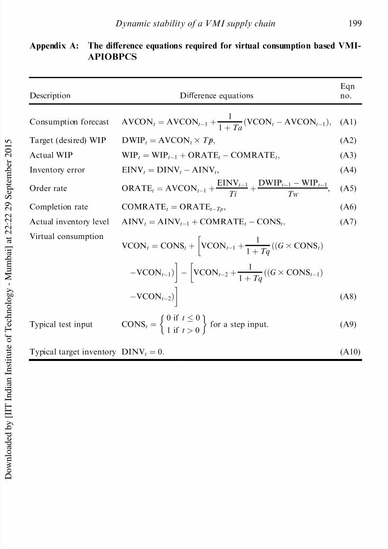
A full description of the dierence equations required is described in Appendix
A. Here, in order to facilitate understanding we will only present the highlights.
6.1. The production delay
A pure time delay for production delay is easily described in the z domain by the
delay operator, z¡Tp . Here, Tp represents the production delay expressed as a mul-
tiple of the sampling interval. The extra unit of time delay in the exponent of theproduction delay in ®gure 4 is used to ensure the proper order of events is obeyed by
the production control system as ®rst outlined by Vassian (1954). It should be noted
that the units of Tp are the same as the sampling interval. For example, if we are
sampling our data system daily, then the production delay should be expressed in
days.
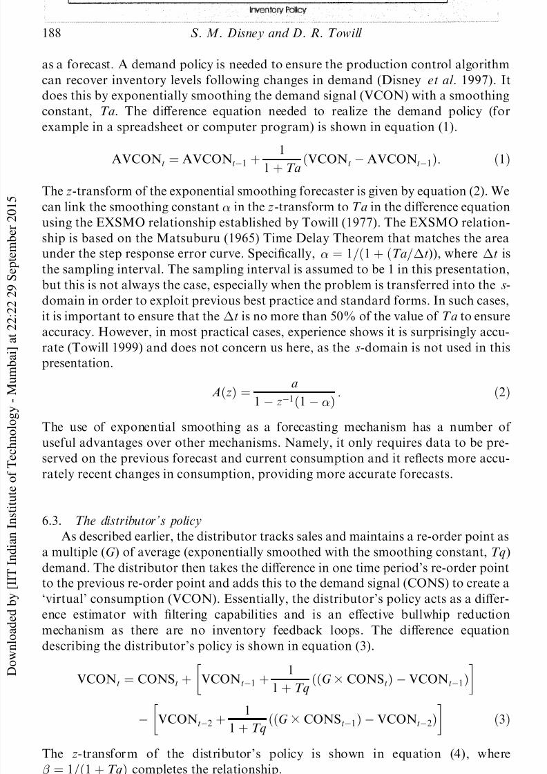
6.2. The demand policy
The demand policy operates at the manufacturers’ echelon. It provides an esti-mate (AVCON) of sales (and stock adjustments Ð to be introduced later) to be used
187Dynamic stability of a VMI supply chain
Figure 4. Block diagram representation of VMI-APIOBPCS.
as a forecast. A demand policy is needed to ensure the production control algorithm
can recover inventory levels following changes in demand (Disney et al . 1997). It
does this by exponentially smoothing the demand signal (VCON) with a smoothing
constant, Ta. The dierence equation needed to realize the demand policy (for
example in a spreadsheet or computer program) is shown in equation (1).
AVCONt ˆ AVCONt¡1 ‡ 1
1 ‡ Ta…VCONt ¡ AVCONt¡1†: …1†
The z-transform of the exponential smoothing forecaster is given by equation (2). We
can link the smoothing constant ¬ in the z-transform to Ta in the dierence equation
using the EXSMO relationship established by Towill (1977). The EXSMO relation-
ship is based on the Matsuburu (1965) Time Delay Theorem that matches the area
under the step response error curve. Speci®cally, ¬ ˆ 1=…1 ‡ …Ta=¢t)), where ¢t is
the sampling interval. The sampling interval is assumed to be 1 in this presentation,but this is not always the case, especially when the problem is transferred into the s-
domain in order to exploit previous best practice and standard forms. In such cases,
it is important to ensure that the ¢t is no more than 50% of the value of Ta to ensure
accuracy. However, in most practical cases, experience shows it is surprisingly accu-
rate (Towill 1999) and does not concern us here, as the s-domain is not used in this
presentation.
A
…z
† ˆ
a
1 ¡ z¡1
…1 ¡ ¬†:
…2
†The use of exponential smoothing as a forecasting mechanism has a number of
useful advantages over other mechanisms. Namely, it only requires data to be pre-
served on the previous forecast and current consumption and it re¯ects more accu-
rately recent changes in consumption, providing more accurate forecasts.
6.3. The distributor’ s policy
As described earlier, the distributor tracks sales and maintains a re-order point asa multiple (G) of average (exponentially smoothed with the smoothing constant, Tq)
demand. The distributor then takes the dierence in one time period’s re-order point
to the previous re-order point and adds this to the demand signal (CONS) to create a
`virtual’ consumption (VCON). Essentially, the distributor’s policy acts as a dier-
ence estimator with ®ltering capabilities and is an eective bullwhip reduction
mechanism as there are no inventory feedback loops. The dierence equation
describing the distributor’s policy is shown in equation (3).
VCONt ˆ CONSt ‡ VCONt¡1 ‡ 1
1 ‡ Tq ……G CONSt† ¡ VCONt¡1†µ ¶¡ VCONt¡2 ‡ 1
1 ‡ Tq……G CONSt¡1† ¡ VCONt¡2†
µ ¶ …3†
The z-transfor m of the distributor’s policy is shown in equation (4), where
System inventory levels are the accumulated sum of the dierence between the
production completion rate and the virtual consumption rate. The dierence equa-
tion required to capture inventory levels is shown in equation (5). The two rates are
converted into the inventory levels in the z domain by the Heaviside Step Function
or the integration term, 1=…1 ¡ z¡1).
AINVt ˆ AINVt¡1 ‡ COMRATEt ¡ V CONt: …5†Information on inventory levels is incorporated into the production order rate
(ORATE). This is achieved by adding a fraction (1=Ti ) of the dierence between
the target inventory level (TINV) and actual inventory level (AINV).
6.5. The pipeline policy
There are signi®cant advantages of incorporating WIP information into theproduction control system as outlined by John et al . (1994), since a stable and
faster response is thereby enabled. Desired work-in-progress (DWIP) levels are set
as a multiple (T · p p) of average virtual consumption (AVCON). T · p p should be set equal
to the production delay, Tp, to ensure inventory levels recover appropriately to
changes in demand, as will be demonstrated later by the Final Value Theorem.
The actual work-in-progress levels (WIP) are calculated as the accumulated sum
of the dierence between production order rate (ORATE) and production comple-
tion rate (COMRATE). The dierence equation required to monitor WIP is shown
in equation (6).
WIPt ˆ WIPt¡1 ‡ ORATEt ¡ COMRATEt: …6†Again, the two rates (ORATE and COMRATE) are translated into the level WIP by
the Heaviside Step Function or the integration term, 1=…1 ¡ z¡1). The pipeline infor-
mation is incorporated into the production order rate by adding a fraction (1=Tw) of
the dierence between desired WIP (DWIP) and actual WIP.
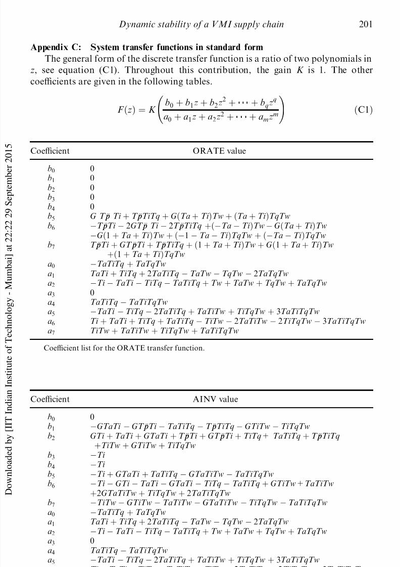
6.6. The block diagram of VMI-APIOBPCS
The block diagram of the VMI-APIOBPCS is shown in ®gure 4. It describes, in a
structured pictorial form, how the individual policies described earlier ®t together to
form the production control system. Manipulating the block diagram, yields `trans-
fer functions’ that describe the relationship between the input (i.e. consumption
(CONS)), and output (i.e. ORATE, COMRATE or AINV) of a system. These z-
domain transfer functions describe completely how the sampled data system behaves
in the time domain.
Of particular interest in the block diagram is the Target systems INVentory
(TINV) and VCON signals. The TINV is a constant that speci®es the desiredsupply chain stock position (i.e. the sum of the Distributor’s stock, the Factory’s
stock and the goods in transit). It should be set by the manufacturer and is a function
of the demand pattern, the distribution lead-time between the two supply chain
echelons (via G), the production and transportation delay, and the desired availabil-
ity at the manufacturer and the distributor. The Virtual CONsumption (VCON)
signal is equal to the actual sales plus net changes in stock at the distributor. If
deliveries were made to the distributor every time period then the VCON would also
be equal to the dispatches between the two echelons. However, the factory does not
have to dispatch goods every time period as the option exists to use less frequent
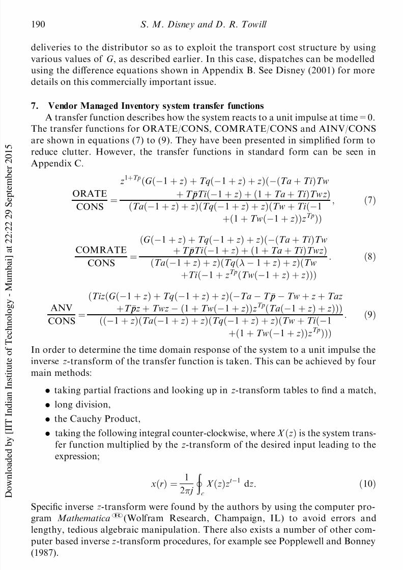
and exploiting L’Hoà pitals’s Rule to ®nd indeterminate solutions where required
shows that ORATE, COMRATE and AINV have an initial value of zero for
VMI-APIOBPCS. This was found also to be the case for APIOPBCS by John et
al . (1994). The ®nal value theorem is a useful tool to determine the long-term tran-
sient behaviour of a transfer function and for the veri®cation of simulations. The
®nal value for ORATE and COMRATE for a stable system is unity, but it can be
very importantly shown that, if the estimate of the production lead-time (T · p p) is not
equal to the actual production lead-time, then there is an oset in ®nal value of the
AINV. Thus, it is important to obtain accurate estimates of Tp. This was also
identi®ed by John et al . (1994) for APIOBPCS. It is for this reason that we suspect
that the Deziel and Eilon (1967) system considers a dierent sequence of events than
the one our model follows. Here, we strictly follow the same order of events as the
popular MIT management game, known as the Beer Game (Sterman 1989), and by
Vassian (1954).
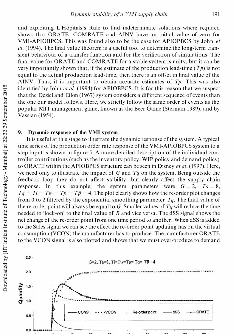
9. Dynamic response of the VMI system
It is useful at this stage to illustrate the dynamic response of the system. A typical
time series of the production order rate response of the VMI-APIOBPCS system to a
step input is shown in ®gure 5. A more detailed description of the individual con-
troller contributions (such as the inventory policy, WIP policy and demand policy)
to ORATE within the APIOBPCS structure can be seen in Disney et al . (1997). Here,
we need only to illustrate the impact of G and Tq on the system. Being outside thefeedback loop they do not aect stability, but clearly aect the supply chain
response. In this example, the system parameters were G ˆ 2, Ta ˆ 8,
Tq ˆ Ti ˆ Tw ˆ Tp ˆ T · p p ˆ 4. The plot clearly shows how the re-order plot changes
from 0 to 2 ®ltered by the exponential smoothing parameter Tq. The ®nal value of
the re-order point will always be equal to G. Smaller values of Tq will reduce the time
needed to `lock-on’ to the ®nal value of R and vice versa. The dSS signal shows the
net change of the re-order point from one time period to another. When dSS is added
to the Sales signal we can see the eect the re-order point updating has on the virtual
consumption (VCON) the manufacturer has to produce. The manufacturer ORATEto the VCON signal is also plotted and shows that we must over-produce to demand
191Dynamic stability of a VMI supply chain
Figure 5. A typical ORATE response to a step input.
dition Ti ˆ Tw, the VMI system will always be robust to end-user intervention. A
similar result can also be found for APIOBPCS. Sample time domain responses
when Ti ˆ Tw to a step input are shown in ®gure 7.
11. Eect of the distribution pattern of the production delay
The general form of a production lag (as opposed to a pure time delay) is shown
in equation (12), (Wikner 1994b). Here, n refers to the order of the production lagand Tp refers to the length of the delay, that is, its pure time delay equivalent
P…z† ˆ nz
Tp…¡1 ‡ z† ‡ nz
n
: …12†
Equation (13) shows the ORATE transfer function derived from the block diagram
if the production delay operator, z¡Tp in ®gure 4 is replaced with the P…z† de®ned by
equation (12) for the case when Tw equals Ti . (Note that the unit delay, z¡1, is still
required to ensure the correct order of events.)
193Dynamic stability of a VMI supply chain
Poles Zeros
Ta
1 ‡ Ta 0
¡1
‡Ti
Ti
Ta‡
T · p p‡
Ti
1 ‡ Ta ‡ Tp ‡ Ti
Tq
1 ‡ Tq
G ‡ Tq
1 ‡ G ‡ Tq
Table 2. Roots of the ORATEtransfer function when Tw ˆ Ti
for VMI-APIOBPCS.
Figure 7. Step response of VMI-APIOBPCS WHEN Tw ˆ Ti
CONS ˆ z…¡Ta ¡ T · p p ¡ Ti ‡ z ‡ Taz ‡ T · p pz ‡ Tiz†…¡G ¡ Tq ‡ z ‡ Gz ‡ Tqz†
…¡Ta ‡ z ‡ Taz†…1 ¡ Ti ‡ Tiz†…¡Tq ‡ z ‡ Tqz† :
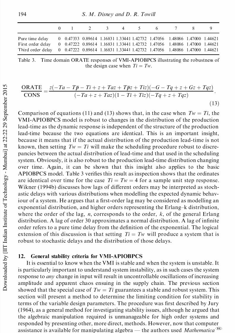
…13†Comparison of equations (11) and (13) shows that, in the case when Tw
ˆTi , the
VMI-APIOBPCS model is robust to changes in the distribution of the production
lead-time as the dynamic response is independent of the structure of the production
lead-time because the two equations are identical. This is an important insight,
because it means that if the actual distribution of the production lead-time is not
known, then setting Tw ˆ Ti will make the scheduling procedure robust to discre-
pancies between the actual distribution of lead-time and that used in the scheduling
system. Obviously, it is also robust to the production lead-time distribution changing
over time. Again, it can be shown that this insight also applies to the basic
APIOBPCS model. Table 3 veri®es this result as inspection shows that the ordinatesare identical over time for the case Ti ˆ Tw ˆ 4 for a sample unit step response.
Wikner (1994b) discusses how lags of dierent orders may be interpreted as stoch-
astic delays with various distributions when modelling the expected dynamic behav-
iour of a system. He argues that a ®rst-order lag may be considered as modelling an
exponential distribution, and higher orders representing the Erlang±k distribution,
where the order of the lag, n, corresponds to the order, k, of the general Erlang
distribution. A lag of order 30 approximates a normal distribution. A lag of in®nite
order refers to a pure time delay from the de®nition of the exponential. The logical
extension of this discussion is that setting Ti ˆ Tw will produce a system that isrobust to stochastic delays and the distribution of those delays.
12. General stability criteria for VMI-APIOBPCS
It is essential to know when the VMI is stable and when the system is unstable. It
is particularly important to understand system instability, as in such cases the system
response to any change in input will result in uncontrollable oscillations of increasing
amplitude and apparent chaos ensuing in the supply chain. The previous section
showed that the special case of Tw ˆ Ti guarantees a stable and robust system. Thissection will present a method to determine the limiting condition for stability in
terms of the variable design parameters. The procedure was ®rst described by Jury
(1964), as a general method for investigating stability issues, although he argued that
the algebraic manipulation required is unmanageabl e for high order systems and
responded by presenting other, more direct, methods. However, now that computer
assistance is available for manipulating algebra Ð the authors used Mathematica1
(Wolfram Research, Champaign, IL) Ð the method will be revisited. This is justi®ed
as it was found that algebraic stability conditions are more easily derived in the last
stage of the methodology presented here.
194 S. M. Disney and D. R. Towill
0 1 2 3 4 5 6 7 8 9
Pure time delay 0 0.47333 0.89614 1.16831 1.33441 1.42732 1.47056 1.48086 1.47000 1.44621
First order delay 0 0.47222 0.89614 1.16831 1.33441 1.42732 1.47056 1.48086 1.47000 1.44621
Third order delay 0 0.47222 0.89614 1.16831 1.33441 1.42732 1.47056 1.48086 1.47000 1.44621
Table 3. Time domain ORATE responses of VMI-APIOBPCS illustrating the robustness of the design case when Ti ˆ Tw.
First, we eliminate all design parameters that do not aect stability. It can be
easily shown that the stability of VMI-APIOBPCS does not depend on Ta, Tq or G
since they appear outside the feedback loops. This result is readily established via
conventional block diagram manipulation (Towill 1970). Note that having selected
stable design parameters, Ta, Tq and G signi®cantly aect the VMI supply chain
response to any particular demand pattern. For subsequent optimization of perform-
ance a procedure based on production adaptation and inventory costs is available
(Disney 2001). Now given that these parameters (Ta, Tq and G) can be set arbitrarily
to inspect stability further, we can choose values that reduce the complexity of the
characteristic equation (G ˆ 0 and Ta ˆ 0 are suitable). In order to avoid solving a
transcendental function it is also necessary to specify a value for Tp, therefore Tp
was set to equal three. T · p p was also set to Tp in order to eliminate inventory osets
over time as proven by John et al . (1994). The ORATE transfer function then
becomes that shown in equation (14),
ORATE
CONS ˆ z3…Ti …3 ‡ Tw†…¡1 ‡ z† ‡ Twz†
Tw ‡ Ti …¡1 ‡ z†…1 ‡ z ‡ z2 ‡ Twz3† : …14†
In order to determine the stability in the z domain it is necessary to inspect each root
to determine if it is outside the unit circle. The problem is that the algebraic solutions
of these high order polynomials involve a very complex mathematical expression
that typically contains lots of trigonometric functions that need inspection. In such
cases, the necessary and sucient conditions to show if the roots lie outside the unit
circle are not easy to determine. Therefore, the Tustin Transformation is taken to
map the z-plane problem into the !-plane. The Tustin transform is shown in equa-
tion (15),
z ˆ ! ‡ 1
¡! ‡ 1: …15†
This changes the problem from determining when the roots lie inside the unit circle
to whether they lie on the left-hand side of the !-plane (Houpis and Lamont 1985).
The !-plane transfer function now becomes equation (16) and the resultant char-acteristic equation (the denominator of the transfer function) is shown in equation
table 5. This is the !-transformed VMI characteristic equation written into the
Routh±Hurwitz Array.
For stability, it is known that a4, a3, ¬1, 1 and ® 1 must all be positive. Inspection
of a4 shows that it is always positive, as it is for a3, ¬1 and ® 1. The case of 1 is more
interesting, as this is the component of the array that can, under certain circum-
stances, become negative. Therefore, in order to determine stability, the relevant
roots of 1 are found for Tw. Plotting this function on the parameter plane yields
®gure 8, which shows the boundary of stability for dierent Tw and Ti for VMI-
APIOBPCS when Tp ˆ T · p p ˆ 3. Figure 8 also highlights six possible designs that are
to be used as test cases of the stability criteria via sample time domain responses to a
unit step input. This result is also true for APIOBPCS. Solving 1 for Ti yields a very
lengthy function but the limiting case of Tw ! 1 (i.e. the stability of IOBPCS)
shows that Ti > 2:24698 also always produces a stable system.
Figure 8 shows the Ti ¡ Tw parameter plane with equation (20) superimposed.Also shown for reference is the Tw ˆ Ti line (the Deziel±Eilon line), which obviously
guarantees a stable APIOBPCS design. The extension to VMI-APIOBPCS is, how-
ever, unique to this paper. We now need to test that our approach utilizing the
Tustin transformation is a good predictor. Hence, for sample values of Tw the
exact step responses of the VMI-APIOBPCS supply chain have been simulated
(see ®gure 9) for stable; critically stable; and unstable designs. These plots con®rm
the theory by clearly identifying the stable region for VMI-APIOBPCS operation. A
196 S. M. Disney and D. R. Towill
s4 a4 a2 a0
s3 a3 a1 0
s2 ¬1 ˆa3a2 ¡ a4a1
a3
¬2 ˆa3 a0 ¡ a4 0
a3
s1 1 ˆ¬1a1 ¡ a3¬2
¬1
2 ˆ 0
s0 ® 1 ˆ 1¬2 ¡ ¬10 1
Table 4. The general Routh±Hurwitz array for afourth-order system.
full-scale optimization methodology for VMI-APIOBPCS is well beyond the scope
of this paper, but is available in Disney (2001). Here, we are concerned with estab-
lishing the stability in the Tw ¡ Ti plane and demonstrating the correctness via
simulation. This has been achieved. In passing, we also note the conservative
nature of the Deziel±Eilon setting of Tw¡
Ti . Furthermore, we have shown an
unexpected bonus to this choice of parameters, namely that the response is then
completely robust to changes in the lead-time distribution.
Therefore the stability conditions for VMI-APIOBPCS and APIOBPCS when
T · p p ˆ Tp ˆ a pure time delay of 3 time units are:
Ti > 2:24698 for Tw ˆ 1 …i:e: no WIP feedback† …20†
or
Tw <¡Ti …¡3 ‡ 4Ti ‡ 2Ti 2† ¡ Ti …¡1 ‡ 2Ti †
1 ‡ 4Ti 2
p 2…1 ¡ Ti ¡ 2Ti 2 ‡ Ti 3† : …21†
14. Conclusions
A VMI-APIOBPCS supply chain has been described using causal loop diagrams,
block diagrams, dierence equations and z-transforms. These have proved to be very
powerful methods for investigating a Vendor Managed Inventor y system. The Final
Value Theorem has demonstrated the importance of obtaining accurate estimates of
the production lead-time, Tp. The time domain behaviour of the system has been
illustrated. It has been shown that if Ti ˆ Tw a stable system that is robust to
changes in the distribution of the production delay is always produced. A procedure
for determining the general stability conditions for VMI-APIOBPCS and
APIOBPCS has also been evaluated by example for the case when T · p p ˆ Tp ˆ 3.
The stability conditions have been presented. The adequacy of the method has been
demonstrated by simulating predicted stable; critically stable and unstable VMI-APIOBPCS designs. Our results con®rm that the predicted instability boundary is
indeed correct. Consequently, the method may be used with con®dence in de®ning
the region in the Tw ¡ Ti parameter plane corresponding to a reasonable stability
margin. Finally, we emphasise the importance of proper timing and matching of the
two feedback loops so as to ensure stable operations. It is thereby shown that the
Deziel±Eilon APIOBPCS setting of Ti ˆ Tw always leads to a conservative design.
Adelson, R. M., 1966, The dynamic behaviour of linear forecasting and scheduling rules.
Operational Research Quarterly, 17(4) 447±462.Aseltine, J . A ., 1958, Transform Methods in Linear System Analysis (York: The Maple Press
Company).Bessler, S. A. and Zehna, P. W., 1968, An application of servomechanisms to inventory.
Navel Research Logistics Quarterly, 15, 137±168.Bissell, C. C., 1996, Control Engineering (London: Chapman & Hall).Bonney, M . C . and Popplewell, K., 1988, Design of production control systems: choice of
systems structure and systems implementation sequence. Engineering Costs and Production Economics, 15, 189±173.
Bonney, M. C., Popplewell, K. and Matoug, M., 1994, Eect of errors and delays in
inventory reporting on production system performance. International Journal of Production Research, 35, 93±105.Burns, J. F. and Sivazlian, B . D ., 1978, Dynamic analysis of multi±echelon supply systems.
Computer and Industrial Engineering, 2, 181±193.Christopher, M., 1992, Logistics and Supply Chain Management: Strategies for Reducing
Costs and Improving Services. (London: Pitman), pp. 166±169.Dejonckheere, J. , Disney, S. M., Lambrecht, M. R. and Towill, D. R., 2000, Matching
your orders to the needs and economies of your supply chain. Proceedings of the 7thEUROMA Conference, Ghent, Belgium, 4±7 June. In R. Van Dierdonck and A.Vereecke (eds), Operations Management ± Crossing Borders and Boundaries: TheChanging Role of Operations, pp. 181±174.
Dejonckheere, J . , Disney, S. M., Lambrecht, M. R. and Towill, D . R ., 2001, Measuringthe bullwhip eect: a control theoretic approach to analyse forecasting inducedBullwhip in order-up-to policies. Working Paper, Cardi University, Wales andLeuven University, Belgium.
Deziel, D . P . and Eilon, S., 1967, A linear production±inventory control rule. TheProduction Engineer, 43, 93±104.
Disney, S. M., 2001, Application of discrete linear control theory to Vendor ManagedInventory. PhD Thesis, Cardi Business School, Cardi University, UK.
Disney, S . M . , Naim, M . M . and Towill, D. R., 1997, Dynamic simulation modeling mod-elling for lean logistics. International Journal of Physical Distribution and Logistics
Management, 27(3), 174±196.
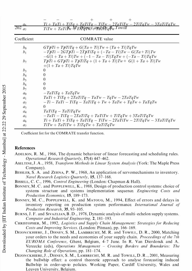
202 S. M. Disney and D. R. Towill
Coecient COMRATE value
b0 GT · p pTi ‡ T · p pTiTq ‡ G…Ta ‡ Ti †Tw ‡ …Ta ‡ Ti †TqTwb1 ¡T · p pTi ¡ 2GT · p pTi ¡ 2T · p pTiTq ‡ …¡Ta ¡ Ti †Tw ¡ G…Ta+Ti †Tw
¡G…1 ‡ Ta ‡ Ti †Tw ‡ …¡1 ¡ Ta ¡ Ti †TqTw ‡ …¡Ta ¡ Ti †TqTwb
Edghill, J. S. and Towill, D. R., 1989, The use of systems dynamics in manufacturingsystems. Trans Inst MC , 11(4), 208±216.
Forrester, J., 1961, Industrial Dynamics (Cambridge, MA: MIT Press).Franklin, G. F., Powell, J. D. and Workman, M. L., 1990, Digital Control of Dynamic
Systems (New York: Addison-Wesley)Grubbstro Èm, R . W ., 1967, On the application of the Laplace Transform to certain economic
problems. Management Science, 13(7), 558±567.Grubbstro Èm, R. W., 1991, A closed-form expression for the net present value of a time±
power cash-¯ow function. Managerial and Decision Economics, 12, 377±381.Grubbstro Èm, R . W ., 1996, Stochastic properties of production±inventory process with
planned production using transform methodology. International Journal of ProductionEconomics, 45, 407±419.
Grubbstro Èm, R. W., 1998, The fundamental equations of MRP theory in discrete time.Working Paper No. 254, Department of Production Economics, LinkoÈ pingUniversity, Sweden.
Grubbstro Èm, R. W. and Tang, O., 2000, Modeling rescheduling activities in a multi-period
production-inventory system. International Journal of Production Economics, 68, 123± 135.
Grubbstro Èm, R. W. and Wang, Z., 2000, Introducing capacity limitations into multi-level,multi-stage production-inventory systems applying input±output/Laplace transformapproach. International Journal of Production Research, 38(17), 4227±4234.
Holmstro Èm, J., 1998, Business process innovation in the supply chain: a case study of imple-menting Vendor Managed Inventory. European Journal of Purchasing and SupplyManagement, 4, 127±131.
Houpis, C . H . and Lamont, G . B ., 1985, Digital Control Systems (New York: McGraw-Hill).John, S. Naim, M. M. and Towill, D. R., 1994, Dynamic analysis of a WIP compensated
decision support system. International Journal of Manufacturing System Design, 1(4),283±297.
Jury, E. I., 1958, Sampled Data Control Systems (New York: Wiley).Jury, E. I.,1964, Theory and Application of the z-Transform Method (New York: Robert E.
Krieger).
Magee, J. F., 1958, Production Planning and Inventory Control (New York: McGraw-Hill),pp. 80±83.
Mason-Jones, R . , Naim, M . M . and Towill, D . R ., 1997, The impact of pipeline control onsupply chain dynamics. International Journal of Logistics Management, 8(2), 47±62.
Matsuburu, M., 1965, On the equivalent deadtime. IEEE Transactions on Automatic
Control , 10, 464±466.McCullen, P. and Towill, D. R., 2000, Practical ways of reducing bullwhip: a case of theGlosuch supply chain. International Journal of Operations Management and Control ,26(10), 24±30.
Naim, M. M. and Towill, D. R., 1995, What’s in the Pipeline? Proceedings of the 2nd International Symposium on Logistics, 11±12 July, pp. 135±142.
Nise, N. S., 1995, Control Systems Engineering (California: Benjamin/Cummings).Popplewell, K. and Bonney, M . C ., 1987, The application of discrete linear control theory
to the analysis of multi-product, multi-level production control system. International Journal of Production Research, 25(1), 45±56.
Simon, H. A., 1952, On the application of servomechanism theory to the study of productioncontrol. Econometrica, 20, 247±268.
Sterman, J., 1989, Modelling managerial behavior: Misperceptions of feedback in a dynamicdecision making experiment. Management Science, 35(3), 321±339.
Tang, O., 2000a, Modelling stochastic lead±times in a production±inventory system using theLaplace transform method. In M. T. Hillery and H. J. Lewis (eds), The 15thInternational Conference on Production Research, ICPR±15 Manufacturing for aGlobal Market, Limerick, Ireland, 9±13 August, 1999, pp. 439±442.
Tang, O. , 2000b, Planning and re-planning within the material requirements planning envir-onment Ð a transform approach. PhD Thesis, Pro®l 16, Linko È ping University, Sweden.
Towill, D. R., 1970, Transfer Function Techniques for Control Engineers (London: Ilie
Towill, D. R., 1977, Exponential smoothing of learning curves. International Journal of Production Research, 15, 1±15.
Towill, D. R., 1982, Dynamic analysis of an inventory and order based production controlsystem. International Journal of Production Research, 20, 369±383.
Towill, D. R., 1999, Fundamental theory of bullwhip induced by exponential smoothingalgorithm. MASTS Occasional Paper No. 61, Cardi University, UK.
Towill, D . R . and Del Vecchio, A., 1994, Application of ®lter theory to the study of supplychain dynamics. Production Planning and Control , 5(1) 82±96.
Towill, D . R . and Yoon, S . S ., 1982, Some features common to inventory system and processcontroller design. Engineering Costs and Production Economics, 6, 225±236.
Towill, D . R . , Lambrecht, M . R . , Disney, S . M . and Dejonckheere, J., 2001, Every supplychain is a ®lter. Proceedings of the 8th EUROMA Conference, Bath, UK, 3±4 June.
Tustin, A., 1953, The Mechanism of Economic Systems (London: William Heinemann).Vassian, H. J., 1954, Application of discrete variable servo theory to inventory control,
Journal of the Operations Research Society of America, 3(3), 272±282.Waller, M. , Johnson, M. E. and Davis, T., 1999, Vendor managed inventory in the retail
supply chain. Journal of Business Logistics, 20(1), 183±203.Wikner, J., 1994a, A discounted cash ¯ow approach in dynamic modelling. Working Paper
220, Department of Production Economics, LinkoÈ ping University, Sweden.Wikner, J., 1994b, Continuous-time dynamic modelling of lead-times. Working Paper 223,
Department of Production Economics, LinkoÈ ping University, Sweden.Wilkinson, S., 1996, Service level and safety stock based on probability. Control , April, 23±
25.Yinzhong, J. and Grubbstro Èm, R.W., 1994, The z-transform in present value analysis:
Utilisation and limitations. Advances in Modelling and Analysis, 19(1), 23±31.