A Distributed Graph Engine for Web Scale RDF Data

Kai Zeng†∗

Jiacheng Yang]∗

Haixun Wang‡ Bin Shao‡ Zhongyuan Wang‡,[

†UCLA ]Columbia University ‡Microsoft Research Asia [Renmin University of China

kzeng@cs.ucla.edu jiachengy@cs.columbia.edu{haixunw, binshao, zhy.wang}@microsoft.com

ABSTRACT

Much work has been devoted to supporting RDF data. Butstate-of-the-art systems and methods still cannot handleweb scale RDF data effectively. Furthermore, many usefuland general purpose graph-based operations (e.g., randomwalk, reachability, community discovery) on RDF data arenot supported, as most existing systems store and index datain particular ways (e.g., as relational tables or as a bitmapmatrix) to maximize one particular operation on RDF data:SPARQL query processing. In this paper, we introduce Trin-ity.RDF, a distributed, memory-based graph engine for webscale RDF data. Instead of managing the RDF data in triplestores or as bitmap matrices, we store RDF data in its na-tive graph form. It achieves much better (sometimes ordersof magnitude better) performance for SPARQL queries thanthe state-of-the-art approaches. Furthermore, since the datais stored in its native graph form, the system can supportother operations (e.g., random walks, reachability) on RDFgraphs as well. We conduct comprehensive experimentalstudies on real life, web scale RDF data to demonstrate theeffectiveness of our approach.

1 Introduction

RDF data is becoming increasingly more available: The se-mantic web movement towards a web 3.0 world is prolif-erating a huge amount of RDF data. Commercial searchengines including Google and Bing are pushing web sitesto use RDFa to explicitly express the semantics of theirweb contents. Large public knowledge bases, such as DB-pedia [9] and Probase [37] contain billions of facts in RDFformat. Web content management systems, which modeldata in RDF, mushroom in various communities all aroundthe world.

Challenges RDF data management systems are facing twochallenges: namely, systems’ scalability and generality. Thechallenge of scalability is particularly urgent. Tremendousefforts have been devoted to building high performance RDF

∗This work is done at Microsoft Research Asia.

Permission to make digital or hard copies of all or part of this work forpersonal or classroom use is granted without fee provided that copies arenot made or distributed for profit or commercial advantage and that copiesbear this notice and the full citation on the first page. To copy otherwise, torepublish, to post on servers or to redistribute to lists, requires prior specificpermission and/or a fee. Articles from this volume were invited to presenttheir results at The 39th International Conference on Very Large Data Bases,August 26th - 30th 2013, Riva del Garda, Trento, Italy.Proceedings of the VLDB Endowment, Vol. 6, No. 4Copyright 2013 VLDB Endowment 2150-8097/13/02... $ 10.00.

systems and SPARQL engines [6, 12, 3, 36, 14, 5, 35, 27].Still, scalability remains the biggest hurdle. Essentially,RDF data is highly connected graph data, and SPARQLqueries are like subgraph matching queries. But most ap-proaches model RDF data as a set of triples, and use RDBMSfor storing, indexing, and query processing. These approachesdo not scale as processing a query often involves a large num-ber of join operations that produce large intermediate re-sults. Furthermore, many systems, including SW-Store [5],Hexastore [35], and RDF-3x [27] are single-machine systems.As the size of RDF data keeps soaring, it is not realis-tic for single-machine approaches to provide good perfor-mance. Recently, several distributed RDF systems, suchas SHARD [29], YARS2 [17], Virtuoso [15], and [20], havebeen introduced. However, they still model RDF data as aset of triples. The cost incurred by excessive join operationsis further exacerbated by network communication overhead.Some distributed solutions try to overcome this limitationby brute-force replication of data [20]. However, this ap-proach simply fails in the face of complex SPARQL queries(e.g., queries with a multi-hop chain), and has a considerablespace overhead (usually exponential).

The second challenge lies in the generality of RDF sys-tems. State-of-the-art systems are not able to support gen-eral purpose queries on RDF data. In fact, most of them areoptimized for SPARQL only, but a wide range of meaningfulqueries and operations on RDF data cannot be expressed inSPARQL. Consider an RDF dataset that represents an en-tity/relationship graph. One basic query on such a graph isreachability, that is, checking whether a path exists betweentwo given entities in the RDF data. Many other queries(e.g., community detection) on entity/relationship data relyon graph operations. For example, random walks on thegraph can be used to calculate the similarity between twoentities. All of the above queries and operations requiresome form of graph-based analytics [34, 28, 22, 33]. Unfor-tunately, none of these can be supported in current RDFsystems, and one of the reasons is that they manage RDFdata in some foreign forms (e.g., relational tables or bitmapmatrices) instead of its native graph form.

Overview of Our Approach We introduce Trinity.RDF,a distributed in-memory RDF system that is capable of han-dling web scale RDF data (billion or even trillion triples).Unlike existing systems that use relational tables (triplestores) or bitmap matrices to manage RDF, Trinity.RDFbuilds on top of a memory cloud, and models RDF datain its native graph form (i.e., representing entities as graphnodes, and relationships as graph edges). We argue thatsuch a memory-based architecture that logically and physi-

265

cally models RDF in native graphs opens up a new paradigmfor RDF management. It not only leads to new optimiza-tion opportunities for SPARQL query processing, but alsosupports more advanced graph analytics on RDF data.

To see this, we must first understand that most graph op-erations do not have locality [23, 31], and rely exclusivelyon random accesses. As a result, storing RDF graphs indisk-based triple stores is not a feasible solution since ran-dom accesses on hard disks are notoriously slow. Althoughsophisticated indices can be created to speed up query pro-cessing, they introduce excessive join operations, which be-come a major cost for SPARQL query processing.

Trinity.RDF models RDF data as an in-memory graph.Naturally, it supports fast random accesses on the RDFgraph. But in order to process SPARQL queries efficiently,we still need to address the issues of how to reduce the num-ber of join operations, and how to reduce the size of inter-mediary results. In this paper, we develop novel techniquesthat use efficient in-memory graph exploration instead ofjoin operations for SPARQL processing. Specifically, we de-compose a SPARQL query into a set of triple patterns, andconduct a sequence of graph explorations to generate bind-ings for each of the triple pattern. The exploration-basedapproach uses the binding information of the explored sub-graphs to prune candidate matches in a greedy manner. Incontrast, previous approaches isolate individual triple pat-terns, that is, they generate bindings for them separately,and make excessive use of costly join operations to com-bine those bindings, which inevitably results in large inter-mediate results. Our new query paradigm greatly reducesthe amount of intermediate results, boosts the query perfor-mance in a distributed environment, and makes the systemscale. We show in experiments that even without a smartgraph partitioning scheme, Trinity.RDF achieves several or-ders of magnitude speed-up on web scale RDF data overstate-of-the-art RDF systems.

We also note that since Trinity.RDF models data as anative graph, we enable a large range of advanced graphanalytics on RDF data. For example, random walks, regu-lar expression queries, reachability queries, distance oracles,community searches can be performed on web scale RDFdata directly. Even large scale vertex-based analytical taskson graph platforms such as Pregel [24] can be easily sup-ported in our system. However, these topics are out of thescope of this paper, and we refer interested readers to theTrinity system [30, 4] for detailed information.

Contributions We summarize the novelty and advantagesof our work as follows.

1. We introduce a novel graph-based scheme for manag-ing RDF data. Trinity.RDF has the potential to sup-port efficient graph-based queries, as well as advancedgraph analytics, on RDF.

2. We leverage graph exploration for SPARQL process-ing. The new query paradigm greatly reduces thevolume of intermediate results, which in turn boostsquery performance and system scalability.

3. We introduce a new cost model, novel cardinality es-timation techniques, and optimization algorithms fordistributed query plan generation. These approachesensure excellent performance on web scale RDF data.

Paper Layout The rest of the paper is organized as fol-lows. Section 2 describes the difference between join oper-ations and graph exploration. Section 3 presents the archi-tecture of the Trinity.RDF system. Section 4 describes howwe model RDF data as native graphs. Section 5 describesSPARQL query processing techniques. Section 6 shows ex-perimental results. We conclude in Section 8.

2 Join vs. Graph Exploration

Joins are the major operator in SPARQL query process-ing. Trinity.RDF outperforms existing systems by orders ofmagnitude because it replaces expensive join operations byefficient graph exploration. In this section, we discuss theperformance implications of the two different approaches.

2.1 RDF and SPARQL

Before we discuss join operations vs. graph exploration, wefirst introduce RDF and SPARQL query processing on RDFdata. An RDF data set consists of statements in the formof (subject, predicate, object). Each statement, also knownas as a triple, is about a fact, which can be interpreted assubject has a predicate property whose value is object. Forexample, a movie knowledge base may contain the followingtriples about the movie “Titanic”:

( T i t an i c , has award , B e s t P i c t u r e )( T i t an i c , c a s t s , L D iCap r i o ) ,( J Cameron , d i r e c t s , T i t a n i c )( J Cameron , wins , Oscar Award ). . .

An RDF dataset can be considered as representing a directedgraph, with entities (i.e. subjects and objects) as nodes, andrelationships (i.e. predicates) as directed edges. SPARQLis the standard query language for retrieving data stored inRDF format. The core syntax of SPARQL is a conjunctiveset of triple patterns called a basic graph pattern. A triplepattern is similar to an RDF triple except that any compo-nent in the triple pattern can be a variable. A basic graphpattern describes a subgraph which a user wants to matchagainst the RDF data. Thus, SPARQL query processing isessentially a subgraph matching problem. For example, wecan retrieve the cast of an award-winning movie directed bya award-winning director using the following query:

Example 1.

SELECT ?movie , ?actor WHERE{?director wins ?award .?director directs ?movie .?movie has_award ?movie_award .?movie casts ?actor .}

SPARQL also contains other language constructs that sup-port disjunctive queries and filtering.

2.2 Using Join Operations

Many state-of-the-art RDF systems store RDF data as a setof triples in relational tables, and therefore, they rely exces-sively on join operations for processing SPARQL queries. Ingeneral, query processing consists of two phases [25]: Thefirst phase is known as the scan phase. It decomposes aSPARQL query into a set of triple patterns. For the queryin Example 1, the triple patterns are ?director wins ?award,?director directs ?movie, ?movie has award ?movie award,and ?movie casts ?actor. For each triple pattern, we scantables or indices to generate bindings. Assuming we are pro-cessing the query against the RDF graph in Figure 1. The

266

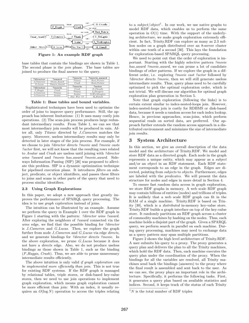
Figure 1: An example RDF graph

base tables that contain the bindings are shown in Table 1.The second phase is the join phase. The base tables arejoined to produce the final answer to the query.

?director ?awardJ Cameron Oscar Award

G Lucas Saturn Award

?director ?movieP Haggis Crash

J Cameron Titanic

J Cameron Avatar

?movie ?movie awardTitanic Best Picture

Crash Best Picture

?movie ?actorCrash D Cheadle

Titanic L Dicaprio

Avatar S Worthington

Star War VI M Hamill

Table 1: Base tables and bound variables.

Sophisticated techniques have been used to optimize theorder of joins to improve query performance. Still, the ap-proach has inherent limitations: (1) It uses many costly joinoperations. (2) The scan-join process produces large redun-dant intermediary results. From Table 1, we can see thatmost intermediary join results will be produced in vain. Af-ter all, only Titanic directed by J Cameron matches thequery. Moreover, useless intermediary results may only bedetected in later stages of the join process. For example, ifwe choose to join ?director directs ?movie and ?movie casts?actor first, we will not know that the resulting rows relatedto Avatar and Crash are useless until joining with ?directorwins ?award and ?movie has award ?movie award. Side-ways Information Passing (SIP) [26] was proposed to allevi-ate this problem. SIP is a dynamic optimization techniquefor pipelined execution plans. It introduces filters on sub-ject, predicate, or object identifiers, and passes these filtersto joins and scans in other parts of the query that need toprocess similar identifiers.

2.3 Using Graph Explorations

In this paper, we adopt a new approach that greatly im-proves the performance of SPARQL query processing. Theidea is to use graph exploration instead of joins.

The intuition can be illustrated by an example. Assumewe perform the query in Example 1 over the RDF graph inFigure 1 starting with the pattern: ?director wins ?award.After exploring the neighbors of ?award connected via thewins edge, we find that the possible binding for ?directoris J Cameron and G Lucas. Then, we explore the graphfurther from node J Cameron and G Lucas via edge directs,and we generate bindings for ?director directs ?movie. Inthe above exploration, we prune G Lucas because it doesnot have a directs edge. Also, we do not produce uselessbindings as those shown in Table 1, such as the binding(P Haggis, Crash). Thus, we are able to prune unnecessaryintermediate results efficiently.

The above intuition is only valid if graph exploration canbe implemented more efficiently than join. This is not truefor existing RDF systems. If the RDF graph is managedby relational tables, triple stores, or disk-based key-valuestores, then we need to use join operations to implementgraph exploration, which means graph exploration cannotbe more efficient than join: With an index, it usually re-quires an O(logN) operation to access the triples relating

to a subject/object1. In our work, we use native graphs tomodel RDF data, which enables us to perform the sameoperation in O(1) time. With the support of the underly-ing architecture, we make graph exploration extremely effi-cient. In fact, Trinity.RDF can explore as many as 2.3 mil-lion nodes on a graph distributed over an 8-server clusterwithin one tenth of a second [30]. This lays the foundationfor exploration-based SPARQL query processing.

We need to point out that the order of exploration is im-portant. Starting with the highly selective pattern ?moviehas award ?movie award, we can prune a lot of candidatebindings of other patterns. If we explore the graph in a dif-ferent order, i.e. exploring ?movie cast ?actor followed by?director directs ?movie, then we will still generate uselessintermediate results. Thus, query plans need to be carefullyoptimized to pick the optimal exploration order, which isnot trivial. We will discuss our algorithm for optimal graphexploration plan generation in Section 5.

Note that graph exploration (following the links) is tocertain extent similar to index-nested-loops join. However,index-nested-loops join is costly for RDBMS or disk-baseddata, because it needs a random access for each index lookup.Hence, in previous approaches, scan-joins, which performsequential reads on sorted data, are preferred. Our ap-proach further extends the random access approach in a dis-tributed environment and minimizes the size of intermediatejoin results.

3 System Architecture

In this section, we give an overall description of the datamodel and the architecture of Trinity.RDF. We model andstore RDF data as a directed graph. Each node in the graphrepresents a unique entity, which may appear as a subjectand/or an object in an RDF statement. Each RDF state-ment corresponds to an edge in the graph. Edges are di-rected, pointing from subjects to objects. Furthermore, edgesare labeled with the predicates. We will present the datastructure for nodes and edges in more detail in Section 4.

To ensure fast random data access in graph exploration,we store RDF graphs in memory. A web scale RDF graphmay contain billions of entities (nodes) and trillions of triples.It is unlikely that a web scale RDF graph can fit in theRAM of a single machine. Trinity.RDF is based on Trin-ity [30], which is a distributed in-memory key-value store.Trinity.RDF builds a graph interface on top of the key-valuestore. It randomly partitions an RDF graph across a clusterof commodity machines by hashing on the nodes. Thus, eachmachine holds a disjoint part of the graph. Given a SPARQLquery, we perform search in parallel on each machine. Dur-ing query processing, machines may need to exchange dataas a query pattern may span multiple partitions.

Figure 2 shows the high level architecture of Trinity.RDF.A user submits his query to a proxy. The proxy generates aquery plan and delivers the plan to all the Trinity machines,which hold the RDF data. Then, each machine executes thequery plan under the coordination of the proxy. When thebindings for all the variables are resolved, all Trinity ma-chines send back the bindings (answers) to the proxy wherethe final result is assembled and sent back to the user. Aswe can see, the proxy plays an important role in the archi-tecture. Specifically, it performs the following tasks. First,it generates a query plan based on available statistics andindices. Second, it keeps track of the status of each Trinity

1N is the total number of RDF triples

267

Figure 2: Distributed query processing framework

machine in query processing by, for example, synchronizingthe execution of each query step. However, each Trinitymachine not only communicates with the proxy. They alsocommunicate among themselves during query execution toexchange intermediary results. All communications are han-dled by a message passing mechanism built in Trinity.

Besides the proxy and the Trinity machines, we also em-ploy a string indexing server. We replace all literals in RDFtriples by their ids. The string indexing server implementsa literal-to-id mapping that translates literals in a SPARQLquery into ids, and an id-to-literal mapping that maps idsin the output back to literals for the user. The mapping canbe either implemented by a separate Trinity in-memory key-value store for efficiency, or by a persistent key-value storeif memory space is a concern. Usually the cost of mappingis negligible compared to that of query processing.

4 Data Modeling

To support graph-based operations including SPARQL querieson RDF data more effectively, we store RDF data in its na-tive graph form. In this section, we describe how we modeland manipulate RDF data as distributed graphs.

4.1 Modeling Graphs

Trinity.RDF is based on Trinity, which is a key-value storein a memory cloud. We then create a graph model on topof the key-value store. Specifically, we represent each RDFentity as a graph node with a unique id, and store it as akey-value pair in the Trinity memory cloud:

(node-id, 〈in-adjacency-list, out-adjacency-list〉) (1)

The key-value pair consists of the node-id as the key, andthe node’s adjacency list as the value. The adjacency listis divided into two lists, one for neighbors with incomingedges and the other for neighbors with outgoing edges. Eachelement in the adjacency lists is a (predicate, node-id) pair,which records the id of the neighbor, and the predicate onthe edge.

Thus, we have created a graph model on top of the key-value store. Given any node, we can find the node-id ofany of its neighbors, and the underlying Trinity memorycloud will retrieve the key-value pair for that node-id. Thisenables us to explore the graph from any given node byaccessing its adjacency lists. Figure 3 shows an example ofthe data structure.

4.2 Graph Partitioning

We distribute an RDF graph across multiple machines, andthis is achieved by the underlying memory cloud, which par-titions the key-value pairs in a cluster. However, due to the

Figure 3: An example of model (1)

characteristics of graphs, we need to look into how the graphis partitioned in order to ensure best performance.

Two factors may have impact on network overhead whenwe explore a graph. The first factor is how the graph ispartitioned. In our system, sharding is supported by theunderlying key-value store, and the default sharding mech-anism is hashing on node-id. In other words, the graph israndomly partitioned. Certainly, sophisticated graph par-titioning methods can be adopted for sharding. However,graph partitioning is beyond the scope of this paper.

The second factor is how we model graphs on top of thekey-value store. The model given by (1) may have poten-tial problems for real-life large graphs. Many real-life RDFgraphs are scale-free graphs whose node degrees follow thepower law distribution. In DBpedia [9], for example, over90% nodes have less than 5 neighbors, while some top nodeshave more than 100,000 neighbors. The model may incur alarge amount of network traffic when we explore the graphfrom a top node x. For simplicity, let us assume none of x’sneighbors resides on the same machine as x does. To visitx’s neighbors, we need to send the node-ids of its neighborsto other machines. The total amount of information we needto send across the network is exactly the entire set of node-ids in x’s adjacency list. For the DBpedia data, in the worstcase, whenever we encounter a top node in graph explo-ration, we need to send 800K data (each node-id is 64 bit)across the network. This is a huge cost in graph exploration.

We take the power law distribution into consideration inmodeling RDF data. Specifically, we model a node x by thefollowing key-value pair:

(node-id, 〈in1, · · · , ink, out1, · · · , outk〉) (2)

where ini and outi are keys to some other key-value pairs:

(ini, in-adjacency-listi) (outi, out-adjacency-listi) (3)

The essence of this model is the following: The key-valuepair (ini, in-adjacency-listi) and the nodes in in-adjacency-listiare stored on the same machine i. In other words, we parti-tion the adjacency lists in model (1) by machine.

The benefits of this design is obvious. No matter howmany neighbors x has, we will send no more than k nids(ini and outi) over the network since each machine i, uponreceiving nidi, can retrieve x’s neighbors that reside on ma-chine i without incurring any network communication. How-ever, for nodes with few neighbors, model (2) is more costlythan model (1). In our work, we use a threshold t to decidewhich model to use. If a node has more than t neighbors, weuse model (2) to map it to the key-value store; otherwise,we use model (1). Figure 4 gives an example with t = 1.Furthermore, in our design, all triples are stored decentral-ized at its subject and object. Thus, update has little costas it only affects a few nodes. However, update is out of thescope of this paper and we omit detailed discussion here.

268

Figure 4: An example of model (2)

4.3 Indexing Predicates

Graph exploration relies on retrieving nodes connected byan edge of a given predicate. We use two additional indicesfor this purpose.

Local predicate indexing We create a local predicate in-dex for each node x. We sort all (predicate, node-id) pairs inx’s adjacency lists first by predicate then by node-id. Thiscorresponds to the SPO or OPS index in traditional RDFapproaches. In addition, we also create an aggregate in-dex to enable us to quickly decide whether a node has agiven predicate and the number of its neighbors connectedby the predicate.

Global predicate indexing The global predicate indexenables us to find all nodes that have incoming or outgoingneighbors labeled by a given predicate. This corresponds tothe PSO or POS index in traditional approaches. Specifi-cally, for each predicate, machine i stores a key-value pair

(predicate, 〈subject-listi, object-listi〉)

where subject-listi (object-listi) consists of all unique sub-jects (objects) with that predicate on machine i.

4.4 Basic Graph Operators

We provide the following three graph operators with whichwe implement graph exploration:

1. LoadNodes(predicate, dir): Return nodes that havean incoming or outgoing edge labeled as predicate.

2. LoadNeighborsOnMachine(node, dir, i): For a givennode, return its incoming or outgoing neighbors thatreside on machine i.

3. SelectByPredicate(nid, predicate): From a given par-tial adjacency list specified by nid, return nodes thatare labeled with the given predicate.

Here, dir is a parameter that specifies whether the pred-icate is an incoming or an outgoing edge. LoadNodes()is straightforward to understand. When it is called, it usesthe global predicate index on each machine to find nodes thathave at least one incoming or outgoing edge that is labeledas predicate.

The next two operators together find specific neighbors fora given node. LoadNeighborsOnMachine() finds a node’sincoming or outgoing neighbors on a given machine. But,instead of returning all the neighbors, it simply returns theini or outi id as given in (2). Then, given the ini or outiid, SelectByPredicate() finds nodes in the adjacency listthat is associated with the given predicate. Certainly, if thenode has less than t neighbors, then its adjacency list is not

distributed, and the two functions simply operate on thelocal adjacency list.

We now use some examples to illustrate the use of theabove 3 operators on the RDF graph shown in Figure 4.LoadNodes(l2, out) finds n2 on machine 1, and n3 on ma-chine 2. LoadNeighborsOnMachine(n0, in, 1) returns thepartial adjacency list’s id in1, and SelectByPredicate(in1, l2)returns n2.

5 Query Processing

In this section, we present our exploration-based approachfor SPARQL query processing.

5.1 Overview

We represent a SPARQL query Q by a query graph G. Nodesin G denote subjects and objects in Q, and directed edgesin G denote predicates. Figure 5 shows the query graphcorresponding to the query in Example 1, and lists the 4triple patterns in the query as q1 to q4.

• q1: (?director wins ?award)

• q2: (?director directs ?movie)

• q3: (?movie has award ?movie award)

• q4: (?movie casts ?actor)

Figure 5: The query graph of Example 1

With G defined, the problem of SPARQL query process-ing can be transformed to the problem of subgraph match-ing. However, as we pointed out in Section 2, existing RDFquery processing and subgraph matching algorithms rely ex-cessively on costly joins, which cannot scale to RDF data ofbillion or even trillion triples. Instead, we use efficient graphexploration in an in-memory key-value store to support fastquery processing. The exploration is conducted as follows:We first decompose Q into an ordered sequence of triplepatterns: q1, · · · , qn. Then, we find matches for each qi,and from each match, we explore the graph to find matchesfor qi+1. Thus, to a large extent, graph exploration acts asjoins. Furthermore, the exploration is carried out on all dis-tributed machines in parallel. In the final step, we gatherthe matchings for all individual triple patterns to the cen-tralized query proxy, and combine them together to producethe final results.

5.2 Single Triple Pattern Matching

We start with matching a single triple pattern. For a triplepattern q, our goal is to find all its matches R(q). Let Pdenote the predicate in q, V denote the variables in q, andB(V ) denote the binding of V . If V is a free variable (notbound), we also use B(V ) to denote all possible values Vcan take. We regard a constant as a special variable withonly one binding.

We use graph exploration to find matches for q. There aretwo ways of exploration: from subject to object (We firsttry to find matches for the subject in q, and then for eachmatch, we find matches for the object in q. We denote thisexploration as −→q ) and from object to subject (We denote

269

this exploration as ←−q ). We use src and tgt to refer to thesource and target of an exploration (i.e., in −→q the src is thesubject, while in ←−q the src is the object).

Algorithm 1 MatchPattern(e)

obtain src, tgt, and predicate p from e (e = −→q or e =←−q )

// On the src side:if src is a free variable then

B(src) =⋃

∀p∈B(P ) LoadNodes(p, dir)

set Mi = ∅ for all i // initialize messages to machine ifor each s in B(src) do

for each machine i donidi = LoadNeighborsOnMachine(s, dir, i)Mi = Mi ∪ (s, nidi)

batch send messages M to all machines

// On the tgt side:for each (s, nid) in M do

for each p in B(P ) doN = SelectByPredicate(nid, p)for each n in N ∩B(tgt) do

R = R ∪ (s, p, n)return R

Algorithm 1 outlines the matching procedure using thebasic operators introduced in Section 4.4. If src is a con-stant, we only need to explore from one node. If src isa variable, we initialize its bindings by calling LoadNodes,which searches the global predicate index to find the matchesfor src. Note that if the predicate itself is a free variable,then we have to load nodes for every predicate. After srcis bound, for each node that matches src and for each ma-chine i, we call LoadNeighborsOnMachine() to find the keynidi. The node’s neighbors on machine i are stored in thekey-value pair with nidi as the key. We then send nidi tomachine i.

Each machine, on receiving the message, starts the match-ing on the tgt side. For each eligible predicate p in B(P ),we filter neighbors in the adjacency list by p by callingSelectByPredicate(). If tgt is a free variable, any neigh-bor is eligible as a binding, so we add (s, p, n) as a matchfor every neighbor n. If tgt is a constant, however, only theconstant node is eligible. As we treat a constant as a spe-cial variable with only one binding, we can uniformly handlethese two cases: we match a new edge only if its target isin B(tgt).

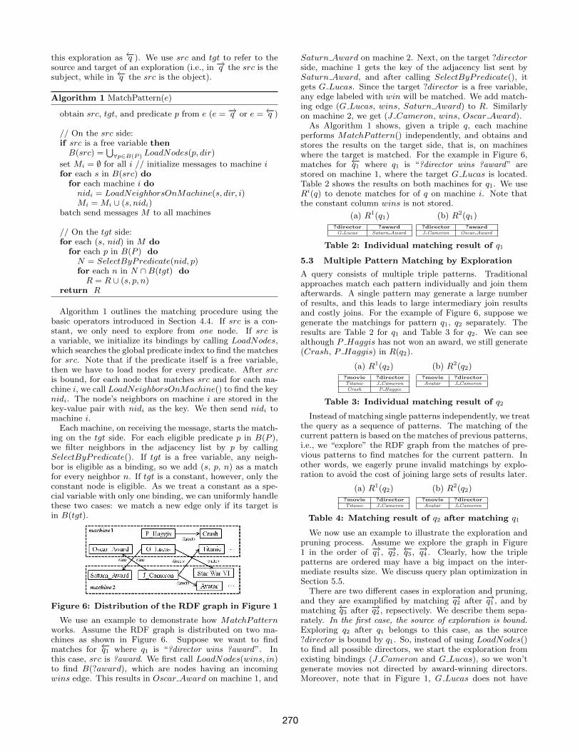
Figure 6: Distribution of the RDF graph in Figure 1

We use an example to demonstrate how MatchPatternworks. Assume the RDF graph is distributed on two ma-chines as shown in Figure 6. Suppose we want to findmatches for ←−q1 where q1 is “?director wins ?award”. Inthis case, src is ?award. We first call LoadNodes(wins, in)to find B(?award), which are nodes having an incomingwins edge. This results in Oscar Award on machine 1, and

Saturn Award on machine 2. Next, on the target ?directorside, machine 1 gets the key of the adjacency list sent bySaturn Award, and after calling SelectByPredicate(), itgets G Lucas. Since the target ?director is a free variable,any edge labeled with win will be matched. We add match-ing edge (G Lucas, wins, Saturn Award) to R. Similarlyon machine 2, we get (J Cameron, wins, Oscar Award).

As Algorithm 1 shows, given a triple q, each machineperforms MatchPattern() independently, and obtains andstores the results on the target side, that is, on machineswhere the target is matched. For the example in Figure 6,matches for ←−q1 where q1 is “?director wins ?award” arestored on machine 1, where the target G Lucas is located.Table 2 shows the results on both machines for q1. We useRi(q) to denote matches for of q on machine i. Note thatthe constant column wins is not stored.

(a) R1(q1)?director ?awardG Lucas Saturn Award

(b) R2(q1)?director ?awardJ Cameron Oscar Award

Table 2: Individual matching result of q1

5.3 Multiple Pattern Matching by Exploration

A query consists of multiple triple patterns. Traditionalapproaches match each pattern individually and join themafterwards. A single pattern may generate a large numberof results, and this leads to large intermediary join resultsand costly joins. For the example of Figure 6, suppose wegenerate the matchings for pattern q1, q2 separately. Theresults are Table 2 for q1 and Table 3 for q2. We can seealthough P Haggis has not won an award, we still generate(Crash, P Haggis) in R(q2).

(a) R1(q2)?movie ?directorTitanic J Cameron

Crash P Haggis

(b) R2(q2)?movie ?directorAvatar J Cameron

Table 3: Individual matching result of q2

Instead of matching single patterns independently, we treatthe query as a sequence of patterns. The matching of thecurrent pattern is based on the matches of previous patterns,i.e., we “explore” the RDF graph from the matches of pre-vious patterns to find matches for the current pattern. Inother words, we eagerly prune invalid matchings by explo-ration to avoid the cost of joining large sets of results later.

(a) R1(q2)?movie ?directorTitanic J Cameron

(b) R2(q2)?movie ?directorAvatar J Cameron

Table 4: Matching result of q2 after matching q1

We now use an example to illustrate the exploration andpruning process. Assume we explore the graph in Figure1 in the order of −→q1 , −→q2 , ←−q3 , −→q4 . Clearly, how the triplepatterns are ordered may have a big impact on the inter-mediate results size. We discuss query plan optimization inSection 5.5.

There are two different cases in exploration and pruning,and they are examplified by matching −→q2 after −→q1 , and bymatching ←−q3 after −→q2 , repsectively. We describe them sepa-rately. In the first case, the source of exploration is bound.Exploring q2 after q1 belongs to this case, as the source?director is bound by q1. So, instead of using LoadNodes()to find all possible directors, we start the exploration fromexisting bindings (J Cameron and G Lucas), so we won’tgenerate movies not directed by award-winning directors.Moreover, note that in Figure 1, G Lucas does not have

270

a directs edge, so exploring from G Lucas will not produceany matching triple. It means we can prune G Lucas safely:There is no need to send the key to its adjacency-list acrossthe network. The results are in Table 4, which containsfewer tuples than Table 3.

In the second case, the target of exploration is bound. Ex-ploring q3 after q2 belongs to this case, as ?movie is boundto {T itanic, Avatar} by −→q2 . We only add results in thisbinding set to the matching results, namely (Best P icture,T itanic). Independently, (Best P icture, Crash) also saties-fies the pattern, but Crash is not in the binding set, soit is pruned. Furthermore, since the previous binding ofAvatar does not match any triple in this round, it is alsosafely pruned from ?movie’s binding. Finally, we incorpo-rate the matches of q3 into the result. As shown in Table 5,it now has three bound variables ?movie, ?director, and?movie award, and contains one row (T itanic, J Cameron,Best P icture) on machine 1 where T itanic is located.

?movie ?director ?movie awardTitanic J Cameron Best Picture

Table 5: Results after incorporating q2 and q3

5.4 Final Join after Exploration

We used two mechanisms to prune intermediate results: abinding is pruned if it cannot reach any bound target, orit cannot be reached from any bound source. Furthermore,once we prune the target (source), we also prune correspond-ing values from the source (target). This greatly reduces thesize of the intermediary results, and does not incur much ad-ditional communication, as shown in the previous example.

However, invalid intermediary results may still remain af-ter the pruning. This is because the pruning of q’s interme-diary results only affects the bindings of q and the immediateneighbors of q. Bindings of other patterns are not consideredbecause otherwise we need to carry all historical bindings inexploration, which incurs big communication cost.

After the exploration finishes, we obtain all the matchesin R. Since R is distributed and may contain invalid results,we gather these results to a centralized proxy and performa final join to assemble the final answer. As we have ea-gerly pruned most of the invalid results in the explorationphase, our join phase is light-weight compared with tradi-tional RDF systems that intensively rely on joins, and wesimply adopt the left-deep join for this purpose.

5.5 Exploration Plan Optimization

Section 5.3 described the query processing for an orderedsequence of triple patterns. The order has significant impacton the query performance. We now describe a cost-basedapproach for finding the optimal exploration plan.

We define an exploration plan as a graph traversal plan,and we denote it as a sequence 〈e1, · · · , en〉, where eachei denotes a directed exploration of a predicate qi in thequery graph, that is, ei = −→qi or ei = ←−qi . The cost ofthe plan is Σicost(ei), where cost(ei), the cost of matching−→qi or ←−qi , is roughly proportional to the size of qi’s results(Section 5.6 will describe cost estimation in more depth).Clearly, the size of qi’s results depends on the matching ofsome qj , j < i. Thus, the total cost depends on the order ofei’s in the sequence.

Naive query plan optimization is costly. There are n! dif-ferent orders for a query graph with n edges, and for each qi,there are two directions of exploration. It is also temptingto adopt the join ordering method in a relational query op-timizer. However, there is a fundamental difference between

our scenario and theirs. In the relational optimizer, laterjoins depend on previous intermediary join results, whilefor us, later explorations depend on previous intermediarybindings. The intermediary join results do not depend onthe order of join, while the intermediary bindings do dependon the order of exploration. For example, consider two plans(1) {−→q1 , −→q2 , ←−q3 , −→q4} and (2) {−→q2 ,−→q3 ,←−q1 ,−→q4}, where the first3 elements are q1, q2, and q3, but in different order. For therelational optimizer (ignore the direction of each qi), the joinresults q1, q2, and q3 are the same no matter how they areordered. But in our case, plan (1) produces {Titanic} andplan (2) produces {Titanic, Crash} for B(?movie), as shownin Table 5. The redundant Crash will makes −→q4 in plan (2)more costly than plan (1).

We now introduce our approach for exploration order op-timization. For a query graph, we find exploration plans forits subgraphs (starting with single nodes), and expand/com-bine the plans until we derive the plan for the entire querygraph. There are two ways to grow a subgraph: expansionand combination. Figure 7(a) depicts an example of expan-sion: we explore to a free variable or a constant and addan edge to the subgraph. The subgraph {q1} is expandedto a larger graph {q1, q2}. Another way to grow a subgraphis that we combine two disjoint subgraphs by exploring anedge starting from one subgraph to the other. Figure 7(b)shows such an example: we combine the subgraph with oneedge q1 with the subplan of q3 by exploring ←−q2 . This way,we construct a larger subgraph from two smaller subgraphs.

(a) Expansion

(b) Combination

Figure 7: Expansion and combination examples

Now, we introduce heuristics for exploration optimization.Let E denote a subgraph, R(E) denote its intermediary joinresults, and B(E) denote the bindings of variables in E . Notethat in our exploration, we compute B(E) only, but notR(E). Furthermore, bindings for some variables in E maycontain redundant values. We define a variable ?c as anexploration point if it satisfies B(c) = ΠcR(E). Intuitively,node ?c is an exploration point if it does not contain anyredundant value, in other words, each of its values mustappear in the intermediary join results R(E). We then adoptthe following heuristics in subgraph expansion/combination.

Heuristic 1. We expand a subgraph from its explorationpoint. We combine two subgraphs by connecting their explo-ration points.

The reason we want to expand/combine at the explorationpoint is because the exploration points do not contain redun-dant values. Hence, they introduce fewer redundant valuesfor other variables in the exploration.

271

After the expansion/combination, we need to determinethe exploration points of the resulting graph. Heuristic 1leads to the following property:

Property 1. We expand a subgraph or combine two sub-graphs through an edge. The two nodes on both ends of theedge are valid exploration points in the new graph.

Proof. For expansion from subgraph E , we start from anexploration point c that satisfies B(c) = ΠcR(E) and explorea new predicate q = c ; c′. Based on our algorithm, wehave ΠcR(e) ⊆ ΠcR(E). Since q /∈ E and c′ /∈ E , we getR(E ∪ q) = R(E) ./c R(q). Thus:

Πc′R(E ∪ q) = Πc′(R(E) ./c R(q))

= Πc′R(q) = B(c′)

which means c′ is an exploration point of E ∪ q. After B(c′)is obtained, the algorithm uses it to prune B(c) so that c’snew binding satisfies B(c) = ΠcR(q). Thus:

ΠcR(E ∪ q) = Πc(R(E) ./c R(q))

= ΠcR(E) ./c ΠcR(q) = ΠcR(q) = B(c)

which means c is a valid exploration point of E∪q. Similarly,we can show Property 1 holds in subgraph combination.

We use dynamic programming (DP) for exploration opti-mization. We use (E , c) to denote a state in DP. We startwith subgraphs of size 1, that is, subgraphs of a single edgeq = u ; v. The states are ({q}, u) and ({q}, v). For theircost, we consider both explorations ←−q and −→q to obtain theminimal cost of reaching the state.

After computing cost for subgraphs of size k, we performexpansion and combination to derive subgraphs of size ≥k+1. Specifically, assuming we are expanding (E , c) throughedge q = c ; v, we reach two states:

(E ∪ {q}, v) and (E ∪ {q}, c) (4)

Let C denote the cost of the state before expansion, and C′

the cost of the state after expansion. We have:

C′ = min{C′, C + cost(−→q )} (5)

Note that: i) We may reach the expanded state in differentways, and we record the minimal cost of reaching the state;ii) C is the cost of state of size ≤ k, which is determinedin previous iterations; iii) If q is in the other direction, i.e.,q = v ; c, then cost(−→q ) above becomes cost(←−q ).

For combining two states (E1, c1) and (E2, c2) where E1 ∩E2 = ∅ through edge q = c1 ; c2, we reach two states:

(E1 ∪ E2 ∪ q, c1) and (E1 ∪ E2 ∪ q, c2) (6)

Let C1 and C2 denote the cost of the two states before com-bination. We update the cost of the combined state to be:

C′ = min{C′, C1 + C2 + cost(−→q )} (7)

We now show the complexity of the DP:

Theorem 1. For a query graph G(V,E), the DP has timecomplexity O(n · |V | · |E|) where n is the number of connectedsubgraphs in G.

Here is a brief sketch-proof: There are n · |V | states in theDP process (each subgraph E can have |E| ≤ |V | nodes),and each update can take at most O(|E|) time.

Theorem 2. Any acyclic query Q with query graph G isguaranteed to have an exploration plan.

We give a brief sketch-proof. Our optimizer resembles theidea of semi-joins although we do not perform join. Bern-stein et al. proved [10] that for any relation in an acyclicquery, there exists a semi-join program that can fully reducethe relation by evaluating each join condition only once. Bymapping each node in G to a relation, and an edge in G toa join condition, we can see that our algorithm can find anexploration plan that evaluates each pattern exactly once.

Discussion. There are two cases we have not consideredformally: i) G is cyclic, and ii) G contains a join on predi-cates. For the first case, our algorithm may not be able tofind an exploration plan. However, we can break a cycle inG by duplicating some variable in the cycle. For example,one heuristic to pick the break point is that we break a cy-cle at node u if it has the smallest cost when we exploreu’s adjacent edges uv1 and uv2 from u; and in the case ofmany cycles, we repeatedly apply this process. The result-ing query graph G′ is acyclic. We can apply our algorithmto search for an approximate plan. For the second case, con-sider a join on predicate (?s ?p ?u), (?x ?p ?y). Here, wecannot explore from the first pattern from bound variables?s or ?u because they are not connected with the secondpattern. To handle this case, after we explore an edge witha variable predicate, we iterate through all unvisited pat-terns sharing the same predicate variable ?p, i.e. (?x ?p ?y),and use LoadNodes to create an initial binding for ?x and?y. This enable us to contine the exploration.

5.6 Cost Estimation

SPARQL selectivity estimation is a challenging task. Stockeret al [32] assumes subject, predicate and object are indepen-dent and the selectivity of each triple is the product of thethree. The result is far from optimal. RDF-3X [25] usestwo approaches: One assumes independence between triplesand relies on traditional join estimation techniques. Theother mines frequent join pathes for large joins and main-tains statistics for these pathes, which is very costly andunfeasible for web-scale RDF data.

We propose a novel estimation method that captures thecorrelation between triples but requires little extra statisticsand data preprocessing. Specifically, we estimate cost(e)where e = −→q or ←−q . In the following, we estimate cost(−→q )only, and the estimation of cost(←−q ) can be obtained in thesame way. Also, we use src and tgt to denote the source andtarget nodes in e. The computation cost of matching q isestimated as the size of the results, namely |R(q)|. Since weoperate in a distributed environment, we model communica-tion cost as well. During exploration, we send bindings andids of adjacency lists across network, so we measure com-munication cost as the binding size of the source node ofthe exploration, i.e. |B(src)|. The final cost(−→q ) is a linearcombination of |R(q)| and |B(src)|.

Now, if we know |B(src)|, we can estimate |R(q)| and|B(tgt)| as

|R(q)| = |B(src)| Cp

Cp(src), |B(tgt)| = |B(src)|Cp(tgt)

Cp(src)

where Cq, Cq(src), Cq(tgt) are the number of triples and con-nected subject/object with predicate p, which can be ob-tained from a single global predicate index look-up. If thepredicate of q is unknown, we consider the average case forall possible predicates. For the case where the source or tar-get of q is constant, we use the local predicate index to geta more accurate estimation.

272

We then derive |B(src)|. For a standalone −→q , we canderive |B(src)| from the global predicate index. When −→q isnot standalone, the binding size of src is affected by relatedpatterns already explored. To capture this correlation, wemaintain a two-dimensional predicate × predicate matrix2.Each cell (i, j) stores four statistics: the number of uniquenodes with predicates pi, pj as its incoming/outgoing edges(4 combinations). When no confusion shall arise, we simplyuse Cpipj to denote the correlation.

As shown in Section 5.5, the query optimizer handles twocases: expansion and combination. In the first case, assumewe expand through a new edge p2 from variable x which isalready connected with p1. Assume the original binding sizeof x is Nx. We have the new binding size N ′

x as

N ′x = Nx

Cp1p2

Cp1

(8)

The second case is combining two edges p1 and p2 on x.Assume the original binding sizes of x with predicate p1 andpredicate p2 are Nx,1 and Nx,2 respectively. We have thenew binding size N ′

x as

N ′x = Nx,1Nx,2

Cp1p2

Cp1Cp2

(9)

For more complex cases in expansion and combinationduring exploration, e.g. expanding a new pattern from asubgraph, or joining two subgraphs, we simply pick the mostselective pair from all pairs of involved predicates.

6 Evaluation

We evaluate Trinity.RDF on both real-life and syntheticdatasets, and compare it against the state-of-the-art central-ized and distributed RDF systems. The results show thatTrinity.RDF is a highly scalable, highly parallel RDF engine.

Systems We implement Trinity.RDF in C#, and deploy iton a cluster, wherein each machine has 96 GB DDR3 RAM,two 2.67 GHz Intel Xeon E5650 CPUs, each with 6 cores and12 threads, and one 40Gb/s InfiniBand Network adaptor.The OS is 64-bit Windows Server 2008 R2 Enterprise withservice pack 1.

We compare Trinity.RDF with centralized RDF-3X [27]and BitMat [8], as well as distributed MapReduce-RDF-3X(a Hadoop-based RDF-3X solution [20]). We deploy thethree systems on machines running 64 bit Linux 2.6.32 usingthe same hardware configuration as used by Trinity.RDF.Just like Trinity.RDF, all of the competitor systems mapliterals to IDs in query processing. But BitMat relies onmanual mapping. For a fair comparison, we measure thequery execution time by excluding the cost of literal/IDmapping. Since all of these three systems are disk-based,we report both their warm-cache and cold-cache time.

Datasets We use two real-life and one synthetic datasets.The real-life datasets are the Billion Triple Challenge 2010dataset (BTC-10) [1] and DBpedia’s SPARQL Benchmark(DBPSB) [2]. The synthetic dataset is the Lehigh Univer-sity Benchmark (LUBM) [16]. We generated 6 datasets ofdifferent sizes using the LUBM data generator v1.7. Wesummarize the statistics of the data and some exemplaryqueries (LUBM queries are also published in [8]) in Table 6

2In many RDF datasets, there is a special predicate rdf:typewhich characterizes the types of entities. Since the numberof entities associated with a certain type varies greatly, wetreat each type as a different predicate.

Dataset #Triples #S/O

BTC-10 3,171,793,030 279,082,615

DBPSB 15,373,833 5,514,599

LUBM-40 5,309,056 1,309,072

LUBM-160 21,347,999 5,259,588

LUBM-640 85,420,588 21,037,012

LUBM-2560 341,888,947 84,202,729

LUBM-10240 1,367,122,031 336,711,191

LUBM-100000 9,956,527,583 2,452,700,932

Table 6: Statistics of datasets used in experiments

BTC-10 S1 S2 S3 S4 S5 S6 S7# of joins 7 5 9 12 6 9 7

DBPSB D1 D2 D3 D4 D5 D6 D7 D8

# of joins 1 1 2 3 3 4 4 5

LUBM L1 L2 L3 L4 L5 L6 L7# of joins 6 1 6 4 1 3 6

Table 7: Statistics of queries used in experiments

and Table 7. All of the queries used in our experiments canbe found online3.

Join vs. Exploration We compare graph exploration (Trin-ity.RDF) with scan-join (RDF-3X and BitMat) on DBPSBand LUBM-160 datasets. The experiment results show thatTrinity.RDF outperforms RDF-3X and BitMat; and moreimportantly, its superiority does not just come from its in-memory architecture, but from the fact that graph explo-ration itself is more efficient than join.

For a fair comparison, we set up Trinity.RDF on a singlemachine, so we have the same computation infrastructurefor all three systems. Specifically, to compare the in-memoryperformance, we set up a 20 GB tmpfs (an in-memory filesystem supported by Linux kernel from version 2.4), anddeploy the database images of RDF-3X and BitMat in thein-memory file system.

The first observation is that managing RDF data in graphform is space-efficient. The database images of LUBM-160and DBPSB in Trinity.RDF are of 1.6G and 1.9G respec-tively, which are smaller or comparable to RDF-3X (2GBand 1.4GB respectively), and are much more efficient thanBitMat (3.6GB and 19GB respectively even without liter-al/ID mapping).

The results on LUBM-160 and DBPSB are shown in Ta-ble 8 and 9. For RDF-3X and BitMat, both in-memoryand on-disk (cold-cache) performances are reported. Trin-ity.RDF outperforms the on-disk performances of RDF-3Xand BitMat by a large margin for all queries: For mostqueries, Trinity.RDF has 1 to 2 orders of magnitude per-formance gain; for some queries, it has 3 orders of magni-tude speed-up. The results from the in-memory performancecomparison are more interesting. Here, since all systems arememory-based, the comparison is solely about graph explo-ration versus scan-join. We can see that the improvementis easily 2-5 fold, and for L4, Trinity.RDF has 3 orders ofmagnitude speed-up. This also shows that, although SIPand semi-join are proposed to overcome the shortcomingsof the scan-join approach, they are not always effective,as shown by L1, L2, L4, D1, D7, etc. Moreover, we varythe complexity of DBPSB queries from 1 join to 5 joins,where Trinity.RDF achieves very stable performance gain.It proves that our query algorithm can effectively find theoptimal exploration order even for complex queries withmany patterns.

We also show that in-memory RDF-3X or BitMat runsslightly better than Trinity.RDF on L2, L3 and D2. Thisis because L2, D2 have very simple structures and few in-termediate results, and Trinity has the overhead due to itsC# implementation.

3http://research.microsoft.com/trinity/Trinity.RDF.aspx

273

L1 L2 L3 L4 L5 L6 L7 Geo. meanTrinity.RDF 281 132 110 5 4 9 630 46RDF-3X (In Memory) 34179 88 485 7 5 18 1310 143BitMat (In Memory) 1224 4176 49 6381 6 51 2168 376RDF-3X (Cold Cache) 35739 653 1196 735 367 340 2089 1271BitMat (Cold Cache) 1584 4526 286 6924 57 194 2334 866

Table 8: Query run-time in milliseconds on the LUBM-160 dataset (21 million triples)

D1 D2 D3 D4 D5 D6 D7 D8 Geo. meanTrinity.RDF 7 220 5 7 8 21 13 28 15RDF-3X (In Memory) 15 79 14 18 22 34 68 35 29BitMat (In Memory) 335 1375 209 113 431 619 617 593 425RDF-3X (Cold Cache) 522 493 394 498 366 524 458 658 482BitMat (Cold Cache) 392 1605 326 279 770 890 813 872 639

Table 9: Query run-time in milliseconds on the DBPSB dataset (15 million triples)

Performance on Large Datasets We experiment on threedatasets, LUBM-10240, LUBM-100000 and BTC-10, to studythe performance of Trinity.RDF on billion scale datasets,and compare it against both centralized and distributedRDF systems. The results are shown in Table 11, 12 and 13.As distributed systems, Trinity.RDF and MapReduce-RDF-3X are deployed on a 5-server cluster for LUBM-10240, a8-server cluster for LUBM-100000 and a 5-server cluster forBTC-10. And we implement the directed 2-hop guaranteepartition for MapReduce-RDF-3X.

BitMat fails to run on BTC-10 as it generates terabytes ofdata for just a single SPO index. Similar issues happen onLUBM-100000. For some datasets and queries, BitMat andRDF-3X fail to return answers in a reasonable time (denotedas “aborted” in our experiment results).

On LUBM-10240 and LUBM-100000, Trinity.RDF getssimilar performance gain over RDF-3X and BitMat as onLUBM-160. Even compared with MapReduce-RDF-3X, Trin-ity.RDF gives surprisingly competitive performance, and forsome queries, e.g. L4-6, Trinity.RDF is even faster. Theseresults become more remarkable if we note that all the LUBMqueries are with simple structures, and MapReduce-RDF-3X specially partitions the data so that these queries canbe answered fully in parallel with zero network communica-tion. In comparison, Trinity.RDF randomly partitions thedata, and has a network overhead. However, data partition-ing is orthogonal to our algorithm and can be easily appliedto reduce the network overhead. This is also evidenced bythe results of L4-6. L4-6 only explore a small set of triples(as shown in Table 14) and incur little network overhead.Thus, Trinity.RDF outperforms even MapReduce-RDF-3X.Moreover, MapReduce-RDF-3X’s partition algorithm incursgreat space overhead. As shown in Table 10, MapReduce-RDF-3X indexes twice as many as triples than RDF-3X andTrinity.RDF do.

LUBM-10240 LUBM-100000 BTC-10

#triple 2,459,450,365 20,318,973,699 6,322,986,673

Overhead 1.80X 2.04X 1.99X

Table 10: The space overhead of MapReduce-RDF-3X compared with the original datasets

The BTC-10 benchmark has more complex queries, somewith up to 13 patterns. In specific, S3, S4, S6 and S7 are notparallelizable without communication in MapReduce-RDF-3X, and additional MapReduce jobs are invoked to answerthe queries. In Table 13, we list separately the time of RDF-3X jobs and MapReduce jobs for MapReduce-RDF-3X. In-terestingly, Trinity.RDF shows up to 2 orders of magnitudespeed-up even over the RDF-3X jobs of MapReduce-RDF-3X. This is probably because MapReduce-RDF-3X divides

a query into multiple subqueries and each subquery pro-duces a much larger result set. This result again provesthe performance impact of exploiting the correlations be-tween patterns in a query, which is the key idea behindgraph exploration.

(a) LUBM group (I) (b) LUBM group (II)

Figure 8: Data scalability

(a) LUBM group (I) (b) LUBM group (II)

Figure 9: Machine scalability

L1 L2 L3 L4 L5 L6 L7

LUBM-160 397 173040 0 10 10 125 7125

LUBM-10240 2502 11016920 0 10 10 125 450721

Table 14: The result sizes of LUBM queries

Scalability To evaluate the scalability of our systems, wecarry out two experiments by (1) scaling the data whilefixing the number of servers, and (2) scaling the numberof servers while fixing the data. We group LUBM queriesinto two categories according to the sizes of their results, asshown in Table 14: (I) Q1, Q2, Q3, Q7. The results of thesequeries increase as the size of the dataset increases. Notethat although Q3 produces an empty result set, it is moresimilar to queries in group (I) as its intermediate result setincreases when the input dataset increases. (II) Q4, Q5,Q6. These queries are very selective, and produce results ofconstant size as the size of dataset increases.

Varying size of data: We test Trinity.RDF running on a3-server cluster on 5 datasets LUBM-40 to LUBM-10240 ofincreasing sizes. The results are shown in Figure 8 (a) and(b). Trinity.RDF utilizes selective patterns to do efficient

274

L1 L2 L3 L4 L5 L6 L7 Geo. meanTrinity.RDF 12648 6018 8735 5 4 9 31214 450RDF-3X (Warm Cache) 36m47s 14194 27245 8 8 65 69560 2197BitMat (Warm Cache) 33097 209146 2538 aborted 407 1057 aborted 5966RDF-3X (Cold Cache) 39m2s 18158 34241 1177 1017 993 98846 15003BitMat (Cold Cache) 39716 225640 9114 aborted 494 2151 aborted 9721MapReduce-RDF-3X (Warm Cache) 17188 3164 16932 14 10 720 8868 973MapReduce-RDF-3X (Cold Cache) 32511 7371 19328 675 770 1834 19968 5087

Table 11: Query run-times in milliseconds for the LUBM-10240 dataset (1.36 billion triples)

L1 L2 L3 L4 L5 L6 L7 Geo. meanTrinity.RDF 176 21 119 0.005 0.006 0.010 126 1.494RDF-3X (Warm Cache) aborted 96 363 0.011 0.006 0.021 548 1.726RDF-3X (Cold Cache) aborted 186 1005 874 578 981 700 633.842MapReduce-RDF-3X (Warm Cache) 102 19 113 0.022 0.016 0.226 51.98 2.645MapReduce-RDF-3X (Cold Cache) 171 32 151 1.113 0.749 1.428 89 13.633

Table 12: Query run-times in seconds for the LUBM-100000 dataset (9.96 billion triples)

pruning. Therefore, Trinity.RDF achieves constant size ofintermediate results and stable performance for group (II)regardless of the increasing data size. For group (I), Trin-ity.RDF scales linearly as the size of the dataset increases,which shows that the network overhead is alleviated by theefficient pruning of intermediate results in graph exploration.

Varying number of machines: We deploy Trinity.RDF inclusters with varying number of machines, and test its per-formance on dataset LUBM-10240. The results are shownin Figure 9 (a) and (b). For group (I), the query time ofTrinity.RDF decrease reciprocally w.r.t. the number of ma-chines. which testifies that Trinity.RDF can efficiently uti-lize the parallelism of a distributed system. Moreover, al-though more partitions increase the amount of intermediatedata delivered across network, our storage model effectivelybounds this overhead. For group (II), due to selective querypatterns, the intermediate results are relatively small. Us-ing more machines does not improve the performance, butagain the performance is very stable and is not impacted bythe extra network overhead.

7 Related Work

Tremendous efforts have been devoted to building high per-formance RDF management systems [12, 36, 14, 5, 35, 27,26, 8, 7, 17]. State-of-the-art approaches can be classifiedinto two categories:

Relational Solutions Most existing RDF systems use arelational model to manage RDF data, i.e. they store RDFtriples in relational tables, and use RDBMS indexing to tunequery processing, which aim solely at answering SPARQLqueries. SW-Store [5] exploits the fact that RDF data hasa small number of predicates. Therefore, it vertically parti-tions RDF data (by predicates) into a set of property tables,maps them onto a column-oriented database, and buildssubject-object index on each property table; Hexastore [35]and RDF-3x [27] manage all triples in a giant triple table,and build indices of all six combinations (SPO, SOP, etc.).

The relational model decides that SPARQL queries areprocessed as large join queries, and most prior systems relyon SQL join optimization techniques for query processing.RDF-3x [27], which is considered the fastest existing sys-tem, proposed sophisticated bushy-join planning and fastmerge join for query answering. However, this approachrequires scanning large fraction of indexes even for veryselective queries. Such redundancy overhead quickly be-comes a bottleneck for billion triple datasets and/or com-plex queries. Several join optimization techniques are pro-posed. SIP (sideways information passing) is a dynamic

optimization technique for pipelined execution plans [26]. Itintroduces filters on subject, predicate, or object identifiers,and passes these filters to other joins and scans in differ-ent parts of the operator tree that need to process similaridentifiers. This introduces opportunities to avoid some un-necessary index scans. BitMat [8] uses a matrix of bitmapsto compress the indexes, and use lightweight semi-join op-erations on compressed data to reduce the intermediate re-sult before actually joining. However, these optimizationsdo not solve the fundamental problem of the join approach.In comparison, our exploration-based approach is radicallydifferent from the join approach.

Graph-based Solutions Another direction of research in-vestigated the possibility of storing RDF data as graphs [18,7, 11]. Many argued that graph primitives besides patternmatching (SPARQL queries) should be incorporated intoRDF languages, and several graph models for advanced ap-plications on RDF data have been proposed [18, 7]. Thereare several non-distributed implementations, including onethat builds an in-memory graph model for RDF data us-ing Jena, and another that stores RDF as a graph in anobject-oriented database [11]. However, both of them aresingle-machine solutions with limited scalability. A relatedresearch area is subgraph matching [13, 40, 19, 39] but mostsolutions rely on complex indexing techniques that are oftenvery costly, and do not have the scalability to process webscale RDF graphs.

Recently, several distributed RDF systems [17, 15, 29,20, 21] have been proposed. YARS2 [17], Virtuoso [15] andSHARD [29] hash partition triples across multiple machinesand parallelize the query processing. Their solutions arelimited to simple index loop queries and do not support ad-vanced SPARQL queries, because of the need to ship dataaround. Huang et al. [20] deploy single-node RDF systemson multiple machines, and use the MapReduce frameworkto synchronize query execution. It partitions and aggres-sively replicates the data in order to reduce network com-munication. However, for complex SPARQL queries, it hashigh time and space overhead, because it needs additionalMapReduce jobs and data replication. Furthermore, Husainet at [21] developed a batch system solely relying on MapRe-duce for SPARQL queries. It does not provide real-timequery support. Yang et al. [38] recently proposed a graphpartition management strategy for fast graph query process-ing, and demonstrate their system on answering SPARQLqueries. However, their work focuses on partition optimiza-tion but not on developing scalable graph query engines.Further, the partitioning strategy is orthogonal to our so-

275

S1 S2 S3 S4 S5 S6 S7 Geo. meanTrinity.RDF 12 10 31 21 23 33 27 21RDF-3X (Warm Cache) 108 8407 27428 62846 32 260 238 1175RDF-3X (Cold Cache) 5265 23881 41819 91140 1041 3065 1497 8101MapReduce-RDF-3X (Warm Cache w/o MapReduce) 132 8 4833 6059 24 1931 2732 453MapReduce-RDF-3X (Cold Cache w/o MapReduce) 2617 661 13755 18712 801 4347 7950 3841MapReduce-RDF-3X (MapReduce) N/A N/A 39928 39782 N/A 33699 33703 36649

Table 13: Query run-times in milliseconds for BTC-10 dataset (3.17 billion triples)

lution and Trinity.RDF can apply their algorithm on datapartitioning to achieve better performance.

8 Conclusion

We propose a scalable solution for managing RDF data asgraphs in a distributed in-memory key-value store. Our queryprocessing and optimization techniques support SPARQLqueries without relying on join operations, and we reportperformance numbers of querying against RDF datasets ofbillions of triples. Besides scalability, our approach also hasthe potential to support queries and analytical tasks thatare far more advanced than SPARQL queries, as RDF datais stored as graphs. In addition, our solution only utilizesbasic (distributed) key-value store functions and thus canbe ported to any in-memory key-value store.

9 References

[1] Billion Triple Challenge.http://challenge.semanticweb.org/.

[2] DBpedia SPARQL Benchmark (DBPSB).http://aksw.org/Projects/DBPSB.

[3] Jena. http://jena.sourceforge.net.[4] Trinity.

http://research.microsoft.com/en-us/projects/trinity/.[5] D. J. Abadi, A. Marcus, S. Madden, and K. Hollenbach.

SW-Store: a vertically partitioned DBMS for SemanticWeb data management. VLDB J., 18(2):385–406, 2009.

[6] S. Alexaki, V. Christophides, G. Karvounarakis,D. Plexousakis, and K. Tolle. The ICS-FORTH RDFSuite:Managing Voluminous RDF Description Bases. InSemWeb, 2001.

[7] R. Angles and C. Gutierrez. Querying rdf data from a graphdatabase perspective. In ESWC, pages 346–360, 2005.

[8] M. Atre, V. Chaoji, M. J. Zaki, and J. A. Hendler. Matrix”Bit” loaded: a scalable lightweight join query processor forRDF data. In WWW, pages 41–50, 2010.

[9] S. Auer, C. Bizer, G. Kobilarov, J. Lehmann, R. Cyganiak,and Z. G. Ives. DBpedia: A Nucleus for a Web of OpenData. In ISWC/ASWC, pages 722–735, 2007.

[10] P. A. Bernstein and D.-M. W. Chiu. Using Semi-Joins toSolve Relational Queries. J. ACM, 28(1):25–40, 1981.

[11] V. Bonstrom, A. Hinze, and H. Schweppe. Storing rdf as agraph. In LA-WEB, pages 27–36, 2003.

[12] J. Broekstra, A. Kampman, and F. van Harmelen. Sesame:A Generic Architecture for Storing and Querying RDF andRDF Schema. In ISWC, 2002.

[13] J. Cheng, J. X. Yu, B. Ding, P. S. Yu, and H. Wang. Fastgraph pattern matching. In ICDE, pages 913–922, 2008.

[14] E. I. Chong, S. Das, G. Eadon, and J. Srinivasan. AnEfficient SQL-based RDF Querying Scheme. In VLDB,2005.

[15] O. Erling and I. Mikhailov. Virtuoso: RDF Support in aNative RDBMS. In Semantic Web InformationManagement, pages 501–519. 2009.

[16] Y. Guo, Z. Pan, and J. Heflin. LUBM: A benchmark forOWL knowledge base systems. Journal of Web Semantics,3(2-3):158–182, 2005.

[17] A. Harth, J. Umbrich, A. Hogan, and S. Decker. Yars2: Afederated repository for querying graph structured datafrom the web. In ISWC/ASWC, pages 211–224, 2007.

[18] J. Hayes and C. Gutierrez. Bipartite graphs as intermediatemodel for rdf. In ISWC, 2004.

[19] H. He and A. K. Singh. Graphs-at-a-time: query languageand access methods for graph databases. In SIGMOD, 2008.

[20] J. Huang, D. J. Abadi, and K. Ren. Scalable SPARQLQuerying of Large RDF Graphs. PVLDB, 4(11), 2011.

[21] M. F. Husain, J. P. McGlothlin, M. M. Masud, L. R. Khan,and B. M. Thuraisingham. Heuristics-Based QueryProcessing for Large RDF Graphs Using Cloud Computing.IEEE Trans. Knowl. Data Eng., 23(9):1312–1327, 2011.

[22] J. Lu, Y. Yu, K. Tu, C. Lin, and L. Zhang. An Approach toRDF(S) Query, Manipulation and Inference on Databases.In WAIM, pages 172–183, 2005.

[23] A. Lumsdaine, D. Gregor, B. Hendrickson, and J. W.Berry. Challenges in Parallel Graph Processing. ParallelProcessing Letters, 17(1):5–20, 2007.

[24] G. Malewicz, M. H. Austern, A. J. C. Bik, J. C. Dehnert,I. Horn, N. Leiser, and G. Czajkowski. Pregel: a system forlarge-scale graph processing. In SIGMOD, 2010.

[25] T. Neumann and G. Weikum. RDF-3X: a RISC-styleengine for RDF. PVLDB, 1(1), 2008.

[26] T. Neumann and G. Weikum. Scalable Join Processing onVery Large RDF Graphs. In SIGMOD, 2009.

[27] T. Neumann and G. Weikum. The RDF-3X engine forscalable management of RDF data. VLDB J., 19(1):91–113,2010.

[28] M. Newman and M. Girvan. Finding and evaluatingcommunity structure in networks. Physical review E,69(2):026113, 2004.

[29] K. Rohloff and R. E. Schantz. High-performance, massivelyscalable distributed systems using the MapReduce softwareframework: the SHARD triple-store. In PSI EtA, 2010.

[30] B. Shao, H. Wang, and Y. Li. The Trinity graph engine.Technical Report 161291, Microsoft Research, 2012.

[31] B. Shao, H. Wang, and Y. Xiao. Managing and mining largegraphs: Systems and implementations. In SIGMOD, 2012.

[32] M. Stocker, A. Seaborne, A. Bernstein, C. Kiefer, andD. Reynolds. SPARQL basic graph pattern optimizationusing selectivity estimation. In WWW, 2008.

[33] Z. Sun, H. Wang, H. Wang, B. Shao, and J. Li. Efficientsubgraph matching on billion node graphs. Proceedings ofthe VLDB Endowment, 5(9):788–799, 2012.

[34] H. Wang, H. He, J. Yang, P. S. Yu, and J. X. Yu. DualLabeling: Answering Graph Reachability Queries inConstant Time. In ICDE, page 75, 2006.

[35] C. Weiss, P. Karras, and A. Bernstein. Hexastore: sextupleindexing for semantic web data management. PVLDB,1(1):1008–1019, 2008.

[36] K. Wilkinson, C. Sayers, H. A. Kuno, and D. Reynolds.Efficient RDF Storage and Retrieval in Jena2. In SWDB,pages 131–150, 2003.

[37] W. Wu, H. Li, H. Wang, and K. Zhu. Probase: Aprobabilistic taxonomy for text understanding. InSIGMOD, 2012.

[38] S. Yang, X. Yan, B. Zong, and A. Khan. Towards effectivepartition management for large graphs. In SIGMODConference, pages 517–528, 2012.

[39] F. Zhu, Q. Qu, D. Lo, X. Yan, J. Han, and P. S. Yu.Mining top-k large structural patterns in a massivenetwork. PVLDB, 4(11):807–818, 2011.

[40] L. Zou, L. Chen, and M. T. Ozsu. Distancejoin: Patternmatch query in a large graph database. PVLDB,2(1):886–897, 2009.

276