Abstract Next-generation scientific applicationsfeature complex workflows comprised of many com-puting modules with intricate inter-module de-pendencies. Supporting such scientific workflows
Q. Wu (B) · X. LuDepartment of Computer Science,University of Memphis,Memphis, TN 38152, USAe-mail: [email protected]
Y. GuDept of Management, Marketing,Computer Science, and Information Systems,University of Tennessee at Martin,Martin, TN 38238, USAe-mail: [email protected]
W. Lin · Y. LiuAtmospheric Science Division, Brookhaven NationalLaboratory, Upton, NY 11793, USA
in wide-area networks especially Grids and op-timizing their performance are crucial to thesuccess of collaborative scientific discovery. Wedevelop a Scientific Workflow Automation andManagement Platform (SWAMP), which enablesscientists to conveniently assemble, execute, mon-itor, control, and steer computing workflowsin distributed environments via a unified web-based user interface. The SWAMP architecture isbuilt entirely on a seamless composition of webservices: the functionalities of its own are pro-vided and its interactions with other tools or sys-tems are enabled through web services for easyaccess over standard Internet protocols while be-ing independent of different platforms and pro-gramming languages. SWAMP also incorporatesa class of efficient workflow mapping schemesto achieve optimal end-to-end performance basedon rigorous performance modeling and algorithmdesign. The performance superiority of SWAMPover existing workflow mapping schemes is jus-tified by extensive simulations, and the systemefficacy is illustrated by large-scale experimentson real-life scientific workflows for climate model-ing through effective system implementation, de-ployment, and testing on the Open Science Grid.
Next-generation e-science features complexworkflows comprised of many computingmodules (also referred to as activities, stages,jobs, transformations, or subtasks in differentcontexts) with intricate inter-module executiondependencies. The execution of such scientificworkflows typically involves the invocation ofa large number and wide variety of distributedprograms or tools for collaborative data analysisand knowledge discovery [60], and also requiresthe use of a wide range of expensive and powerfulresources including supercomputers, PC clusters,high-end workstations, experimental facilities,large-screen display devices, high-performancenetwork infrastructures, and massive storagesystems. Typically, these resources are deployedat various research institutes and national labo-ratories, and are provided to users through wide-area network connections that may spanthrough several countries [10, 19, 36, 61], henceinevitably exhibiting an inherent dynamic naturein their availability, reliability, capacity, andstability.
As new computing technologies and network-ing services rapidly emerge, enabling functional-ities are progressing at an ever-increasing pace,unfortunately, so are the dynamics, scale, hetero-geneity, and complexity of the networked comput-ing environment. Supporting large-scale scientificworkflows in distributed heterogeneous networkenvironments is crucial to ensuring the successof mission-critical scientific applications and max-imizing the utilization of massively distributedcomputing and networking resources. However,application users, who are primarily domainexperts, oftentimes need to manually exploitavailable resources, and configure and run theircomputing tasks over networks using softwaretools they are familiar with based on their ownempirical studies, inevitably leading to unsatisfac-tory performance in such diverse and dynamicenvironments.
We propose to develop a Scientific Work-flow Automation and Management Platform
(SWAMP1) to support the distributed execu-tion and management of large-scale scientificworkflows in heterogeneous network environ-ments. Compared to the previous work in [76], wehave made significant and substantial changes toboth the design and implementation of the system:
– The entire SWAMP architecture has beencompletely redesigned and re-implementedusing distributed web services for a seam-less integration instead of individual softwarepackages installed on the user site.
– The workflow execution mode has beenchanged from Condor’s default centralizeddata forwarding mechanism to the distributeddirect inter-module data transfer using Storkfor improved end-to-end performance.
– The previous system employs an extremelysimplified modeling method that uses theprocessor frequency to represent the node’sprocessing power; while the new system takesa rigorous statistical approach that considersa combination of both hardware and softwareproperties to model and predict the perfor-mance of various types of scientific computa-tions with a higher accuracy.
– In addition to the algorithm for delay min-imization in unitary processing applications,the workflow mapping component in the newsystem has incorporated a set of specially-designed algorithms for throughput maximiza-tion in streaming applications.
Within SWAMP, a scientific workflow is mod-eled as a Directed Acyclic Graph (DAG) whereeach vertex represents a computing moduleand each directed edge represents the execu-tion dependency between two adjacent modules.Each module is considered as an autonomous
1A preliminary version of the SWAMP development [76]was published in Proc. of the 6th Int. Workshop on Sys.Man. Tech., Proc., and Serv., in conjunction with IPDPS,Atlanta, GA, April 19, 2010.
Distributed Workflow Management System 369
computing agent: it receives data as input fromone or more preceding modules, executes a pre-defined processing routine on the aggregate inputdata, and sends the results as output to one ormore succeeding modules. We assume that nei-ther can a module start execution until all therequired inputs arrive nor send out the resultsuntil the execution is completed on each dataset.The current version of SWAMP integrates agraphical toolkit based on a unified web interfacefor abstract workflow composition, employs Con-dor/DAGMan [12] for workflow dispatch, andadopts Stork [64] for direct inter-module datatransfer to realize completely distributed execu-tion without centralized data forwarding. The goalof SWAMP is to pool geographically distributedbut Internet connected computing resources to-gether to enable and accelerate the executionof computation-intensive scientific workflows inwide-area networks.
The SWAMP architecture is entirely built on aseamless composition of web services: the func-tionalities of its own are provided and its in-teractions with other tools or systems are facili-tated through web services for easy access overstandard Internet protocols while being indepen-dent of different platforms and programming lan-guages. SWAMP also incorporates a specially-designed mapping engine that automatically mapsabstract workflows to underlying networks toachieve Minimum End-to-end Delay (MED) forunitary (one-time) processing applications andMaximum Frame Rate (MFR) for streaming ap-plications based on real-time network measure-ments and system status monitoring [28, 73]. Thecore of this mapping engine consists of a classof workflow mapping optimization schemes de-veloped through rigorous performance modelingand algorithm design. The performance superior-ity of SWAMP over existing workflow mappingschemes is justified by extensive simulations, andthe system efficacy is illustrated by large-scaleworkflow experiments on a real-life scientific ap-plication for climate modeling through effectivesystem implementation, deployment, and testingon the Open Science Grid [48].
The rest of the paper is organized as follows:In Section 2, we conduct a survey of related work.The SWAMP framework and functional compo-nents are described in Section 3. The performancemodeling and prediction approach is introducedin Section 4. The workflow mapping algorithmsare presented in Section 5. The system implemen-tation details and performance evaluations areprovided in Section 6. We conclude our work inSection 7.
2 Related Work
With the advent of next-generation e-science, aplethora of frameworks and tools have been dev-eloped for generating, refining, and executing sci-entific workflows. Such efforts include P-GRADE[33], Pegasus [15], Kepler [40], Condor/DAGMan[12], Taverna [30], Triana [9], Swift [65], JavaCoG Kit [37], Sedna [71], and SWAMP [76].Each workflow system has its own language, de-sign suite, and software components, and the sys-tems vary widely in their execution models andthe kinds of components they coordinate [14].Some systems attempt to provide general-purposeworkflow functionalities while others are moregeared toward specific applications and are op-timized to support specific component libraries.Google’s MapReduce provides a software frame-work to support distributed computing on clus-ters of computers [13]. Since its primary goalis to process large datasets through a partition-composition approach using the map and reduc-tion operations, MapReduce does not sufficientlymeet the requirement of distributed scientificworkflows that typically consist of different com-putational jobs executed in wide-area networks.
Many existing systems support workflow exe-cution in Grid environments, which provide com-positional programming and execution modelsto enable resource interactions by supplying themechanisms to access, aggregate, and managethe network-based infrastructure of science [32].Such Grid-based scientific applications includeLarge Hadron Collider (LHC) supported by the
370 Q. Wu et al.
Worldwide LHC Computing Grid (WLCG) [72],climate modeling supported by the Earth SystemGrid (ESG) [20], and NASA’s National AirspaceSimulation supported by the Virtual NationalAirspace Simulation (VNAS) Grid [32, 43]. Manyother Grid systems such as Open Science Grid(OSG) [48], ASKALON [21, 66], TeraGrid, andGridCOMP (see [17] for a more complete list)are under rapid development and deployment.These existing workflow or Grid systems havea primary design goal to provide services or in-frastructures for coordinated application interop-eration, distributed job submission, or large datatransfer, but generally there lacks a comprehen-sive workflow solution that integrates workflowmapping schemes to support large-scale scientificapplications for end-to-end performance opti-mization. Furthermore, most systems using abatch scheduler are not inherently capable of sup-porting streaming applications that require com-putational steering, which is a critical activity inexplorative sciences where the parameter valuesof an online simulation or a computing modulemust be changed and determined on a realistictime scale.
Over the years, the workflow mapping prob-lems in heterogeneous network environmentshave been increasingly identified and investigatedby many researchers to facilitate more conve-nient and comprehensive collaborations amongdifferent institutes and domains across wide-areanetworks [6, 8, 16, 31, 55]. Existing workflowmapping algorithms can be roughly classified intothe following five categories [42, 69]: (i) Graph-based methods [11, 44]. Among the traditionalgraph mapping problems in theoretical aspects ofcomputing, subgraph isomorphism is known to beNP-complete while the complexity of graph iso-morphism still remains open. (ii) List schedulingtechniques, in which the most commonly used iscritical path method [34, 41, 54]. (iii) Clustering al-gorithms [6, 24], which assume an unlimited num-ber of processors and thus are not very feasible forpractical use. (iv) Duplication based algorithms[3, 7, 55], most of which are of a prohibitively highcomplexity. (v) Guided random search methodssuch as genetic algorithm [4, 70] and simulatedannealing [59], where additional efforts are often
required to determine an appropriate terminationcondition and usually there is no performanceguarantee.
Most workflow mapping or task schedulingproblems in Grid environments or multiproces-sor systems assume complete networks, homoge-neous resources, and specific mapping constraints.Our work differs from the above efforts in severalaspects: (i) We investigate the workflow map-ping problems for both MED and MFR. (ii) Wetarget computer networks of arbitrary topologywith heterogeneous computer nodes and networklinks. (iii) We consider resource sharing amongmultiple concurrent module executions on thenode or data transfers over the link. (iv) We em-ploy a statistical approach to performance mod-eling and prediction. (v) We build the SWAMPsystem on web services for easy access and en-hanced interoperability across different platforms.(vi) We implement and integrate our mappingoptimization algorithms into the SWAMP systemand test them with real-life scientific workflows onGrids.
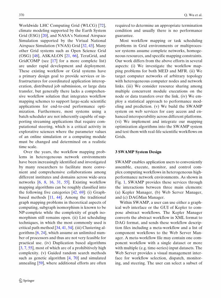
3 SWAMP System Design
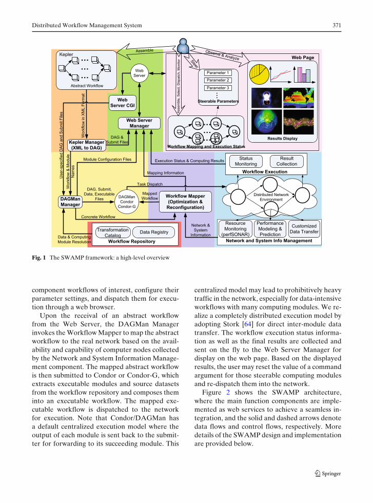
SWAMP enables application users to convenientlyassemble, execute, monitor, and control com-plex computing workflows in heterogeneous high-performance network environments. As shown inFig. 1, SWAMP provides these services throughthe interactions between three main elements:(a) Kepler Manager, (b) Web Server Manager,and (c) DAGMan Manager.
Within SWAMP, a user can use either a graph-ical web interface or the GUI of Kepler to com-pose abstract workflows. The Kepler Managerconverts the abstract workflow in XML format toDAG format, and sends these workflow descrip-tion files including a meta-workflow and a list ofcomponent workflows to the Web Server Man-ager. A meta-workflow file may contain one com-ponent workflow with a single dataset or morewith multiple (e.g. time-series) input datasets. TheWeb Server provides a visual management inter-face for workflow selection, dispatch, monitor-ing, and steering. The user can select a subset of
Distributed Workflow Management System 371
Fig. 1 The SWAMP framework: a high-level overview
component workflows of interest, configure theirparameter settings, and dispatch them for execu-tion through a web browser.
Upon the receival of an abstract workflowfrom the Web Server, the DAGMan Managerinvokes the Workflow Mapper to map the abstractworkflow to the real network based on the avail-ability and capability of computer nodes collectedby the Network and System Information Manage-ment component. The mapped abstract workflowis then submitted to Condor or Condor-G, whichextracts executable modules and source datasetsfrom the workflow repository and composes theminto an executable workflow. The mapped exe-cutable workflow is dispatched to the networkfor execution. Note that Condor/DAGMan hasa default centralized execution model where theoutput of each module is sent back to the submit-ter for forwarding to its succeeding module. This
centralized model may lead to prohibitively heavytraffic in the network, especially for data-intensiveworkflows with many computing modules. We re-alize a completely distributed execution model byadopting Stork [64] for direct inter-module datatransfer. The workflow execution status informa-tion as well as the final results are collected andsent on the fly to the Web Server Manager fordisplay on the web page. Based on the displayedresults, the user may reset the value of a commandargument for those steerable computing modulesand re-dispatch them into the network.
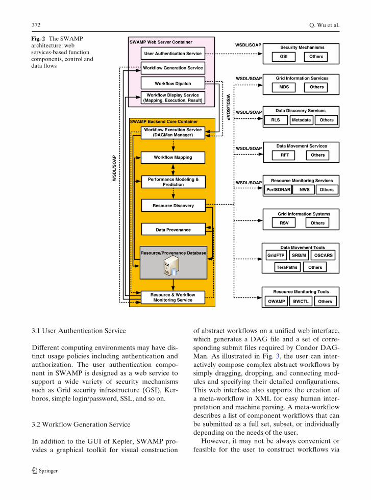
Figure 2 shows the SWAMP architecture,where the main function components are imple-mented as web services to achieve a seamless in-tegration, and the solid and dashed arrows denotedata flows and control flows, respectively. Moredetails of the SWAMP design and implementationare provided below.
372 Q. Wu et al.
Fig. 2 The SWAMParchitecture: webservices-based functioncomponents, control anddata flows
SWAMP Web Server Container
Workflow Display Service (Mapping, Execution, Result)
WSDL/SOAP
SWAMP Backend Core Container
Workflow Execution Service(DAGMan Manager)
WS
DL
/SO
AP
Grid Information Services
Data Discovery Services
Data Movement Services
Metadata
Resource Monitoring Services
Resource Monitoring Tools
PerfSONAR
Others
WSDL/SOAP
WSDL/SOAP
WSDL/SOAP
WSDL/SOAP
Performance Modeling & Prediction
Resource/Provenance Database
Grid Information Systems
Data Movement Tools
GridFTP
TeraPaths
OWAMP BWCTL
SRB/M OSCARS
Others
WS
DL
/SO
AP
Workflow Dipatch
Workflow Generation Service
User Authentication ServiceSecurity Mechanisms
Workflow Mapping
Resource Discovery
Data Provenance
Resource & WorkflowMonitoring Service
MDS Others
Others
Others
Others
Others
RLS
RFT
NWS
OthersGSI
RSV
3.1 User Authentication Service
Different computing environments may have dis-tinct usage policies including authentication andauthorization. The user authentication compo-nent in SWAMP is designed as a web service tosupport a wide variety of security mechanismssuch as Grid security infrastructure (GSI), Ker-boros, simple login/password, SSL, and so on.
3.2 Workflow Generation Service
In addition to the GUI of Kepler, SWAMP pro-vides a graphical toolkit for visual construction
of abstract workflows on a unified web interface,which generates a DAG file and a set of corre-sponding submit files required by Condor DAG-Man. As illustrated in Fig. 3, the user can inter-actively compose complex abstract workflows bysimply dragging, dropping, and connecting mod-ules and specifying their detailed configurations.This web interface also supports the creation ofa meta-workflow in XML for easy human inter-pretation and machine parsing. A meta-workflowdescribes a list of component workflows that canbe submitted as a full set, subset, or individuallydepending on the needs of the user.
However, it may not be always convenient orfeasible for the user to construct workflows via
Distributed Workflow Management System 373
Fig. 3 The web-based workflow generation by dragging, dropping and connecting modules and specifying their detailedconfigurations
the graphical toolkit in the web browser for ap-plications where a large number of modules areinvolved, or a collection of workflows need to begenerated by combining the parameters in a par-ticular way specified by domain experts. SWAMPprovides a workflow generation web service to au-tomatically generate such workflows. The inputsto this web service are partial workflow represen-tations that describe the input files, the executa-bles (workflow components) and their parame-ters, as well as the output files produced by theseexecutables. For example, the workflow structureand module information specified through theweb interface in Fig. 3 can be directly sent tothe web service for automatic workflow genera-tion. This service also requests the informationon datasets from the web interface and avail-able computing resources from the resource andworkflow monitoring service.
The outputs of both interactive and automaticworkflow generations are workflow descriptionfiles in XML format. Scientists are also allowed tocustomize the workflows by modifying the steer-
able parameters through the web interface afterthe workflows are dispatched.
3.3 Workflow Execution Service
The workflow execution component is imple-mented as a web service, which receives the ab-stract workflow description files from its client, i.e.the workflow dispatch component. The workflowexecution service needs to contact resource andworkflow monitoring service to place callbackto the workflow display service for dispatchedworkflows. If the workflow execution service failsto place the callback, it will prevent the workflowfrom dispatching. Otherwise, the workflow execu-tion service proceeds to perform workflow map-ping, generates the desired workflow and job de-scription files, and dispatches the workflows tothe Condor environment. The workflow executionservice serves as a portal to the Condor batchsystem and its main goal is to simplify the processof real workflow submission and execution.
374 Q. Wu et al.
Fig. 4 Condor pool architecture
SWAMP allows users to submit jobs by usinga specified repository that stores all input data aswell as existing output data. A job can also besubmitted using a shared file system to directlyaccess input and output files. In the latter case,the job or module must be able to access the datafiles from any machine, on which it is deployedthrough either NFS or AFS. SWAMP providesaccess to Condor’s own native mechanisms forGrid computing as well as other Grid systems,e.g. through Condor-G when Grid universe jobsare sent to Grid resources utilizing Globus soft-ware for job execution. The Globus Toolkit pro-vides a framework for building Grid systems andapplications.
Figure 4 shows a local Condor pool architec-ture. Each execution node in the SWAMP condorpool accepts a new job only if the load of thesystem is not too high and there is enough mem-
ory available for efficient execution. The jobs aresubmitted to the “schedd” process, which storesthem in a permanent storage and advertises theirneeds. The “startd” process on an execution nodeadvertises its resources to the “collector” process.The “negotiator” process regularly fetches theseadvertisements (ClassAds) from the “collector”and “schedd”, and assigns jobs to execution nodes.For every such association, a shadow and a starterprocess are created and all further communica-tions take place between these two entities.
Figure 5 shows the execution procedure ofSWAMP in Grid environments. In order to sub-mit jobs to Grid resources, the submit machineneeds to apply for a certificate from a trusted Cer-tificate Authority (CA) for authentication. Thesubmit machine with all Grid software installedand configured manages the jobs running on theGrid. Before running jobs on the Grid, we needto ensure that the submit machine is able to ob-tain the correct user proxy, which is presented toremote Grid sites during authentication. Condor-G stages data and submits jobs to the Gatekeeperat a remote Grid site. Globus GRAM on theGatekeeper authenticates users, sends jobs to thelocal resource manager such as Condor, PBS, andFork, and notifies users of job statuses. The exe-cution machines run the jobs and notify the localresource managers of job statuses.
Each workflow supported by SWAMP has anoutput module that runs after all other user mod-ules have completed. The main task of this outputmodule is to send the final output to the Web
Fig. 5 The executionprocedure of SWAMP inGrid environments
Distributed Workflow Management System 375
Server. Instead of creating a separate daemon, weadd this extra job as part of the DAG workflow forfinal output sending to avoid checking the Condorlog files or invoking Condor’s management com-mand in polling mode. In Condor batch system,jobs with higher numerical priority run before jobswith lower numerical priority. To send the finaloutput to the user promptly, the output module isassigned with the highest priority.
3.4 Performance Modeling and Prediction
In order to improve the quality of workflow ex-ecution, we investigate the problem of modelingscientific computations and predicting their exe-cution time based on a combination of both hard-ware and software properties. The performancemodeling and prediction component queries theresource and provenance database to retrieve theinformation of computing resources, datasets andexecutables, or interacts with the resource discov-ery component to collect such information. In thiscomponent, we employ statistical learning tech-niques to estimate the effective computationalpower of a given computer node at any time pointand compute the total number of CPU cyclesneeded for executing a given computational pro-gram on any input data size. The technical detailsof this component are provided in Section 4.
3.5 Workflow Mapping
The efficiency of the SWAMP system largelydepends on the performance of the mappingschemes that map computing workflows to net-work nodes in the Condor pool, which is deter-mined by the Condor job dispatch scheme. Themapping scheme currently employed by the Con-dor scheduler works as a matchmaker of Clas-sAds. Condor schedules job dispatch by match-ing the requests for both machine ClassAds andjob ClassAds. In addition to the Condor pool,SWAMP is capable of mapping workflows onto avariety of target resources such as those managedby Portable Batch System (PBS) [53] and LoadSharing Facility (LSF) [39], with an improvedmapping performance by incorporating a set ofwell-designed mapping schemes into the Condornegotiator daemon.
The workflow mapping component obtains theinformation on computing modules such as the ex-ecutables and data from the resource and prove-nance database, and then converts an abstractworkflow to an executable workflow based onthe prediction of the module execution time usingthe performance modeling and prediction compo-nent. The mapping objective is to select an appro-priate set of computer nodes in the network andassign each computing module in the workflowto one of those selected nodes to achieve MEDfor fast response and MFR for smooth data flow.The workflow mapping algorithms are presentedin Section 5.
3.6 Resource Discovery
The resource discovery component interacts withan extensive set of existing services and systems toacquire information on data, computing and net-working resources, and data movement tools, allof which is stored in the resource and provenancedatabase.
The data discovery process involves two steps:(i) Use data attributes specified by users to querya metadata service, which maps the specified at-tributes into a list of logical file names. (ii) Usethese logical names to query existing registry ser-vices such as the Globus Replica Location Service(RLS) [25] to locate the replicas of the requireddata.
The resource discovery component also com-municates with information services and systemsto discover available computing resources andcorresponding characteristics such as the numberof CPUs, CPU frequency, queueing length, andavailable disk space. Currently supported infor-mation services and systems include Monitoringand Discovery Service (MDS) [45], Resource andSite Validation (RSV) [50], and so on.
This component queries a number of resourcemonitoring services and tools to monitor the sta-tus of the networking resources, including perf-SONAR [52], Network Weather Service (NWS)[46], One-Way Active Measurement Protocol(OWAMP) [47], and Bandwidth Test Controller(BWCTL) [5].
In order to improve the performance of largedata transfer in wide-area networks, the resource
376 Q. Wu et al.
discovery component also queries other infor-mation services to locate and employ the avail-able data movement services and tools, includingGridFTP [26], Reliable File Transfer (RFT) [57],Storage Resource Broker (SRB) [62], StorageResource Management (SRM) [63], On-demandSecure Circuit Advance Reservation System(OSCARS) [49], and TeraPaths [67].
3.7 Data Provenance
The data management in heterogeneous networkssuch as OSG [48] is a key component of thearchitecture and service of the common infrastruc-ture. Large-scale scientific applications have ledto unprecedented levels of data collection, whichmake it very difficult to keep track of the datageneration history. The data provenance compo-nent provides information about the derivationhistory of data starting from its original sources.It enables scientists to verify the correctness oftheir simulations and reproduce them if neces-sary. SWAMP provides provenance informationrelated to workflow module execution by ana-lyzing the log files of the Condor system. Theselog files contain execution information of eachmodule, such as location, time, and output, all ofwhich are stored in the resource and provenancedatabase.
3.8 Resource and Workflow Monitoring Service
The resource and workflow monitoring serviceuses the callback placed by the workflow execu-tion service to trigger the data provenance com-ponent to keep track of the workflow executionprogress. It also queries the resource and prove-nance database to obtain the status informationof the computing resources, and then sends theabove information on the fly to the workflowdisplay service to update the web interface.
3.9 Workflow Display Service
Each workflow eventually generates an output.The ability to view and manage the output dataas soon as it is produced is valuable to usersfor result interpretation. Users can keep track ofthe real time information of workflow mapping,
execution and result through the web interface.The workflow display service component instan-taneously updates the web interface using the in-formation provided by the resource and workflowmonitoring service component. The ability to re-dispatch workflows and return the immediatefeedback allows the user to modify parameters ofany dispatched workflow and re-dispatch individ-ual workflows that require further computation.SWAMP uses coloring convention to indicate theexecution status of a module and supports a tab-ular fashion to show the statistical information ofthe modules and the links.
4 A Statistical Approach to PerformanceModeling and Prediction
Finding a good workflow mapping scheme crit-ically depends on an accurate prediction of theexecution time of each individual module in theworkflow. The time prediction of a scientific com-putation does not have a silver bullet as it isdetermined collectively by several dynamic sys-tem factors including concurrent loads, memorysize, CPU speed, and also by the complexityof the computational program itself. To tacklethe problem of modeling scientific computationsand predicting their execution time, we employ aperformance model that takes into account bothhardware and software properties, which is thenused by the prediction method for predicting orestimating the execution time of a given computa-tional job on any computer.
In [18], Dobber et al. provided a broad sur-vey of existing prediction methods and also pro-posed a Dynamic Exponential Smoothing (DES)method for job runtime prediction on sharedprocessors. All the methods in [18] are solelybased on the statistical analysis of historical run-time measurements of user jobs. Although alsoemploying a statistical method, our performancemodeling and prediction take a fundamentallydifferent approach using benchmark machineswith the main goal to accurately describe the rela-tionship between the runtime of a given scientificcomputation and various system factors includingthe hardware properties of the computing nodeand the software properties of the program. Since
Distributed Workflow Management System 377
these methods are based on different inputs un-der different assumptions, their prediction perfor-mances may not be directly comparable.
Let vector H(t) represent the hardware profileof a given machine that consists of both staticconfiguration and dynamic usage information attime t, defined as:
H(t) = hstatic ∪ hdynamic(t) (1)
where hstatic denotes the set of static propertiesand hdynamic(t) denotes the set of dynamic prop-erties at time point t. Typically, the hardwarespecifications of the machine are considered staticwhile the workloads on the machine are dynamicin nature, therefore resulting in a time-varyinglevel of resource capacity. For convenience, wetabulate in Table 1 the notations used in ourperformance model.
Let Ch represent the ef fective processing (EP)power provided by the available hardware re-sources of the machine. The EP power determinesthe number of usable CPU cycles (i.e. the totalnumber of CPU cycles minus those used for sys-tem overheads and other background workloads).The relationship between the hardware profileand Ch can be described as:
Ch(t) = H(t) · θh + ϑh (2)
Table 1 Notations used in the performance model
Symbol Meaning
H(t) The total hardware resources on the machinein the presence of concurrent workloadsat time point t
hstatic The set of static hardware properties of themachine
hdynamic(t) The set of dynamic hardware properties attime point t
S The set of software properties of thecomputational job
Ch The effective processing powerCs The total number of CPU cycles required
by the computational jobθh The coefficient vector for hardware
estimationθs The coefficient vector for software
estimation
where θh is the coefficient vector of a regressionestimate for hardware profiles, and ϑh denotes theset of regression constants.
Now let us consider the software properties ofthe computational job and estimate the number Cs
of CPU cycles that are needed to execute the job.Similarly, we employ a polynomial regression tocapture the relationship between Cs and the job’ssoftware properties:
Cs = S · θs + ϑs (3)
where S denotes the vector holding the softwareproperties of the program (computational job), θs
is the coefficient vector of a regression estimatefor software properties, and ϑs denotes the set ofregression constants.
Given Ch and Cs, the relationship between theexecution time and the hardware and softwareproperties is still very complicated. We employ anonlinear parametric regression analysis methodto model such complex behaviors. The estimationof the job execution time T(t) on the machine attime point t is given by:
T(t) = f ((Ch(t)θ1 + Csθ2), β) + ϑ, (4)
where θ1 and θ2 are the coefficient vectors of aregression estimate for the hardware and soft-ware properties, respectively. Equation (4) can berewritten in the following form:
T(t) = f (X0) · β ′ + ϑ, (5)
where X0 denotes Ch(t)θ1 + Csθ2. Equation (5) islinear in terms of the explanatory variable β
′, and
the dimension of the vector class estimator is thesame as the dimension of X0.
For a given computational job running on agiven machine, we assume that the available hard-ware resources H(t) on the machine and the jobexecution time T(t) on that machine be distrib-uted by a joint probability distribution PH(t),T(t).Note that the software properties of a computa-tional job remain constant, and therefore the totalnumber of CPU cycles required for running thejob is fixed for a given input data size. Note thatthe actual runtime of some algorithms (especiallyfor optimization purposes) may depend on boththe input size and the input data. Since our sys-tem is focused on scientific applications and the
378 Q. Wu et al.
complexity of scientific computations is largelydetermined by the dimensional parameters andthe number of iterations, our approach is still ap-plicable in most science domains (especially withvolume data processing such as visualization),
Now by using the least squares estimate, wecalculate the execution time estimation error as:
Iθ,ϑ =∫
(T̂(t) − T(t))dPH(t),T(t), (6)
where T̂(t) denotes the actual amount of timetaken. The best estimator for the actual executiontime is given by minimizing (6). In order to obtainthe best estimation, one would need an accuratedistribution PH(t),T(t), which is very hard to find inpractice. The problem may not be tractable if thisdistribution is complex [75].
Let I∗θ,ϑ denote the best estimation given by (6):
I∗θ,ϑ = min(Iθ,ϑ ). (7)
The goal of the estimation is to have a highprobability that the estimation error is withinsome permissible limit ε. Using the result from thesample size estimation [56], we have:
P((Iθ,ϑ − I∗θ,ϑ ) > ε) ≤ 1 − 8
(64eε
ln64eε
)d
e−ε2 k512 ,
(8)
where k is the sample size.As mentioned in [75], the same argument holds
on the estimation bound. Note that this estimationbound does not depend on the form of distributionPH(t),T(t), but the drawback is that it only ensuresthe closeness of the estimation error to the bestpossible linear approximation. It is possible thatthe latter itself may not be unsatisfactory if theunderlying relationship is non-linear.
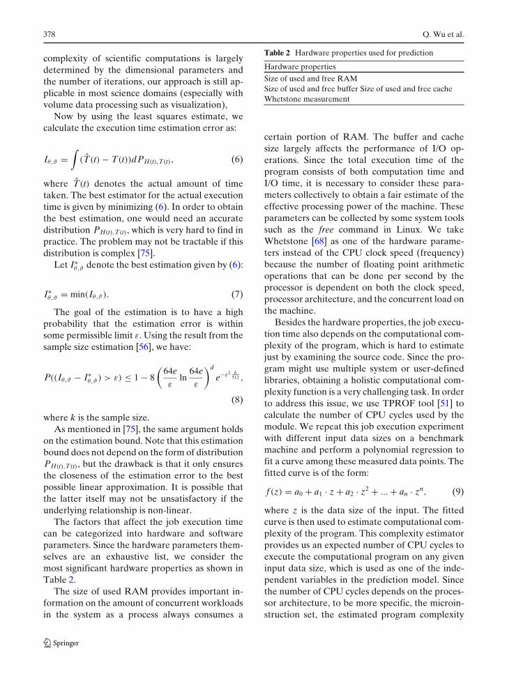
The factors that affect the job execution timecan be categorized into hardware and softwareparameters. Since the hardware parameters them-selves are an exhaustive list, we consider themost significant hardware properties as shown inTable 2.
The size of used RAM provides important in-formation on the amount of concurrent workloadsin the system as a process always consumes a
Table 2 Hardware properties used for prediction
Hardware properties
Size of used and free RAMSize of used and free buffer Size of used and free cacheWhetstone measurement
certain portion of RAM. The buffer and cachesize largely affects the performance of I/O op-erations. Since the total execution time of theprogram consists of both computation time andI/O time, it is necessary to consider these para-meters collectively to obtain a fair estimate of theeffective processing power of the machine. Theseparameters can be collected by some system toolssuch as the free command in Linux. We takeWhetstone [68] as one of the hardware parame-ters instead of the CPU clock speed (frequency)because the number of floating point arithmeticoperations that can be done per second by theprocessor is dependent on both the clock speed,processor architecture, and the concurrent load onthe machine.
Besides the hardware properties, the job execu-tion time also depends on the computational com-plexity of the program, which is hard to estimatejust by examining the source code. Since the pro-gram might use multiple system or user-definedlibraries, obtaining a holistic computational com-plexity function is a very challenging task. In orderto address this issue, we use TPROF tool [51] tocalculate the number of CPU cycles used by themodule. We repeat this job execution experimentwith different input data sizes on a benchmarkmachine and perform a polynomial regression tofit a curve among these measured data points. Thefitted curve is of the form:
f (z) = a0 + a1 · z + a2 · z2 + ... + an · zn, (9)
where z is the data size of the input. The fittedcurve is then used to estimate computational com-plexity of the program. This complexity estimatorprovides us an expected number of CPU cycles toexecute the computational program on any giveninput data size, which is used as one of the inde-pendent variables in the prediction model. Sincethe number of CPU cycles depends on the proces-sor architecture, to be more specific, the microin-struction set, the estimated program complexity
Distributed Workflow Management System 379
needs to be adjusted appropriately on a machinewith a different architecture, for example, by cal-culating and applying the ratio of the requiredCPU cycles for performing the same floating-point operation (flop) between the current ma-chine and the benchmark machine. The predic-tion model is built using a multivariate nonlinearregression function which takes estimated CPUcycles, and hardware parameters shown in Table2 as independent variables and estimates theamount of time module takes on the machine. Theprediction model is of the form:
T = A( f (z))
B(I), (10)
where T is the dependent variable which repre-sents time taken by the executable, I representsthe independent variables. Once its regressionform is determined, f (z) produces a concretevalue for a given input data size z. However,directly using this value (the estimated numberof CPU cycles) may not yield an accurate timeprediction because the actual number of CPUcycles allocated to a job execution may be subjectto a certain variation, for example, due to fre-quent page swapping if the program requires morememory space than what is available. The functionA(·) is in the form of A(x) = p0 + p1 · xk0 + p2 ·xk1 + ... + pn · xkn−1 where p0....pn, k0...kn are realnumbers, and the purpose of using this functionis to capture such variations. Similarly, we use apolynomial function B(·) formed by taking all pos-sible combinations of the independent variables Ito capture the effect of each independent variablewhen acting alone and in combination of otherindependent variables. In the simplest case withtwo dependent variables, x1 and x2, a possibleform of the first order the function B(·) could takeis B(x1, x2) = p0 + p1 · x1 + p2 · v2 + p3 · (v1 · v2).
The estimated computational complexity ofthe module using polynomial regression in (9)does not indicate the inherent parallelism of themodule.
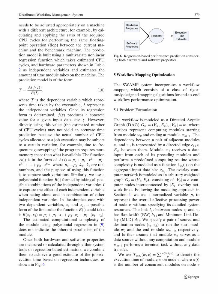
Once both hardware and software propertiesare measured or calculated through either systemtools or regression-based estimators, we combinethem to achieve a good estimate of the job ex-ecution time based on regression techniques, asshown in Fig. 6.
Fig. 6 Regression-based performance prediction consider-ing both hardware and software properties
5 Workflow Mapping Optimization
The SWAMP system incorporates a workflowmapper, which consists of a class of rigor-ously designed mapping algorithms for end-to-endworkflow performance optimization.
5.1 Problem Formulation
The workflow is modeled as a Directed AcyclicGraph (DAG) Gw = (Vw, Ew), |Vw| = m, wherevertices represent computing modules startingfrom module w0 and ending at module wm−1. Thedependency between a pair of adjacent moduleswi and w j is represented by a directed edge ei, j ∈Ew between them. Module w j receives a datainput from each of its preceding modules andperforms a predefined computing routine whosecomplexity is modeled as a function λw j(·) on theaggregate input data size zw j . The overlay com-puter network is modeled as an arbitrary weightedgraph Gc = (Vc, Ec), consisting of |Vc| = n com-puter nodes interconnected by |Ec| overlay net-work links. Following the modeling approach inSection 4, we use a normalized variable pi torepresent the overall effective processing powerof node vi without specifying its detailed systemresources. The link li, j between nodes vi and v j
has Bandwidth (BW) bi, j and Minimum Link De-lay (MLD) di, j. We specify a pair of source anddestination nodes (vs, vd) to run the start mod-ule w0 and the end module wm−1, respectively,and further assume that module w0 serves as adata source without any computation and modulewm−1 performs a terminal task without any datatransfer.
We use Texec(w, v) = ∑ α(t)·δw(t)p to denote the
execution time of module w on node v, where α(t)is the number of concurrent modules on node v
380 Q. Wu et al.
during t, δw(t) = pα(t)t denotes the amount of
partial module execution completed during timeinterval [t, t + t] when α(t) remains unchanged,and λw(zw) = ∑
δw(t) is the total computationalrequirement of module w. We use Ttran(e, l) =∑ β(t)·δe(t)
b + d to denote the data transfer time ofdependency edge e over network link l, where β(t)is the number of concurrent data transfers overlink l during t, δe(t) = b
β(t)t denotes the amountof partial data transfer completed during timeinterval [t, t + t] when β(t) remains unchanged,and ze = ∑
δe(t) is the total data transfer sizeof dependency edge e. Note that computing andnetworking resources could be shared by multi-ple modules and edges that are processing andtransferring different input datasets. Due to thedynamics in concurrent workload on nodes andconcurrent traffic over links, both α(t) and β(t) aretime-varying in nature.
Based on the analytical cost models, we con-sider two performance metrics:
(i) End-to-end Delay (ED), which is the totalcompletion time of the entire workflow fromthe time when a single dataset is fed intothe first module to the time when the finalresult is generated at the last module. Oncea mapping scheme is determined, the ED iscalculated as the total time cost incurred onthe critical path (CP), i.e. the longest path.We denote the set of contiguous modules onthe CP that are allocated to the same nodeas a “group”, and refer to those moduleslocated on the CP as “critical” modules andothers as “branch” or “non-critical” mod-ules. A general mapping scheme divides theCP into q (1 ≤ q ≤ m) contiguous groupsgi, i = 0, 1, · · · , q − 1 of critical modules andmaps them to a network path P of not neces-sarily distinct q nodes, vP[0], vP[1], · · · , vP[q−1]from source vs = vP[0] to destination vd =vP[q−1]. The ED of a mapped workflow isdefined as:
TED(CP mapped to a path P of q nodes
)
= Texec + Ttran =q−1∑i=0
Tgi +q−2∑i=0
Te(gi,gi+1)
=q−1∑i=0
⎛⎝ ∑
j∈gi, j≥1
(∑ α j(t) · δw j(t)
pP[i]
)⎞⎠
+q−2∑i=0
(∑ βe(gi,gi+1)(t) · δe(gi,gi+1)(t)b P[i],P[i+1]
+ dP[i],P[i+1])
, (11)
where e(gi, gi+1) denotes the edge fromgroup gi to gi+1 mapped to link lP[i],P[i+1]between nodes vP[i] and vP[i+1].
(ii) Frame Rate (FR) or throughput, i.e. the in-verse of the global Bottleneck Time (BT)of the workflow. The bottleneck time TBT
could be either on a node or over a link,defined as:
TBT(Gw mapped to Gc)
= maxwi∈Vw,e j,k∈Ew
vi′ ∈Vc,l j′ ,k′ ∈Ec
(Texec(wi, vi′),
Ttran(e j,k, l j′,k′)
)
= maxwi∈Vw,e j,k∈Ew
vi′ ∈Vc,l j′ ,k′ ∈Ec
⎛⎝
∑ αi(t)·δwi (t)pi′
,∑ β j,k(t)·δe j,k (t)
b j′ ,k′ + d j′,k′
⎞⎠ .
(12)
We assume that the inter-module communi-cation cost on the same node is negligible.
Since the execution start time of a module de-pends on the availability of its input datasets, themodules assigned to the same node may not runsimultaneously. The same is also true for concur-rent data transfers over the same network link.The workflow mapping problem with arbitrarynode reuse for MED or MFR is formally definedas follows: Given a DAG-structured computingworkf low Gw = (Vw, Ew) and a heterogeneouscomputer network Gc = (Vc, Ec), we wish to f inda mapping scheme that assigns each computingmodule to a network node such that the mappedworkf low achieves:
MED = minall possible mappings
(TED) , (13)
MFR = maxall possible mappings
(1
TBT
). (14)
Distributed Workflow Management System 381
Note that MED is the minimum sum of timecosts along the CP while MFR is achieved by iden-tifying and minimizing the time TBT on a globalbottleneck node or link among all possible map-pings. We maximize FR to produce the smoothestdata flow in streaming applications when multipledatasets are continuously generated and fed intothe workflow.
5.2 Design of Mapping Algorithms
A workflow mapping scheme must account forthe temporal constraints in the form of execu-tion order of computing modules and spatial con-straints in the form of geographical distribution ofnetwork nodes and their connectivity. The gen-eral DAG mapping problem is known to be NP-complete [2, 22, 35, 38] even on two processorswithout any topology or connectivity restrictions[1], which rules out any polynomial optimal so-lutions. We incorporate two efficient workflowmapping algorithms into the SWAMP system tooptimize workflow performance in terms of MEDand MFR.
For unitary processing applications, we incor-porate into our system an improved RecursiveCritical Path (impRCP) algorithm [74], which re-cursively chooses the CP based on the previousround of calculation and maps it to the networkusing a dynamic programming (DP)-based pro-cedure until the mapping results converge to anoptimal or suboptimal point. For the sake of com-pleteness, we provide a brief summary of thosekey steps in the impRCP algorithm:
1. Assume the network topology to be completewith identical computing nodes and communi-cation links, and determine the initial comput-ing/transfer time cost components.
2. Find the CP of the workflow with initial timecost components using a longest path algo-rithm.
3. Remove the assumption on resource homo-geneity and connectivity completeness, andmap the current CP to the actual networkusing the optimal pipeline mapping algorithmbased on a DP-based procedure for MED witharbitrary node reuse as proposed in [29].
4. Map non-critical modules using A∗ and BeamSearch algorithms.
5. Compute a new CP using updated time costcomponents and calculate the new MED.
Steps 2–5 are repeated until a certain condition ismet, for example, the difference between a newMED resulted from the current mapping and anold MED resulted from the previous mappingis less than a preset threshold. The complexityof impRCP is O(ρ · m · n · |Ew|), where ρ is thepredefined beam width in the BS algorithm, mand |Ew| are the number of modules and edges inthe workflow, respectively, and n is the number ofnodes in the network.
For streaming applications with serial data in-puts, we incorporate into our system a Layer-oriented Dynamic Programming algorithm [27],referred to as LDP, which maps workflows tonetworks by identifying and minimizing the globalBT to achieve the smoothest dataflow. The keyidea of LDP is to first sort a DAG-structuredworkflow in a topological order and then mapcomputing modules to network nodes on a layer-by-layer basis, while taking into considerationboth module dependency in the workflow andnode connectivity in the network. We use a two-dimensional DP table to record the intermediatemapping result at each step where a module ismapped layer-by-layer to a strategically selectednetwork node, where the horizontal coordinatesrepresent the sequence numbers of topologicallysorted modules, and the vertical coordinates rep-resent the labels of nodes starting from the sourcenode vs to the destination node vn−1.
To reduce the search complexity, we proposea Greedy LDP, which selects the best node ineach column that yields the minimum global BTfor mapping the current module, hence fillingone cell only in each column. In Greedy LDP,we recursively calculate the minimum BT of thesub-solution that maps the subgraph (a partialworkflow) consisting of the current module w j
and all the modules before the current layer tothe network until the last module wm−1 is reachedand mapped to the destination vd, which is repre-sented by the right bottom cell in the DP table.The complexity of this algorithm is O(l · n · |Ew|),
382 Q. Wu et al.
where l is the number of layers in the topologicallysorted workflow, n is the number of nodes in thenetwork, and |Ew| is the number of edges in theworkflow.
6 System Implementation and Evaluation
We conduct extensive comparative performanceevaluations based on both simulations and ex-periments through system implementation andreal deployment to illustrate the performancesuperiority of the proposed solution over otherworkflow mapping algorithms and the Condordefault execution model.
6.1 Simulation-based Performance Evaluation
The proposed impRCP and Greedy LDP mappingalgorithms are implemented in C++. For perfor-mance comparison, we also implement three exist-ing algorithms, namely (i) Greedy A∗ [58], whichmaps subtasks onto a large number of sensornodes based on A∗ algorithm, whose complexityis O(m2 + kn(m − k)), where m is the number ofmodules, n is the number of sensor nodes, and
k is the number of modules in the independentset; (ii) Streamline (SL) [2], which maximizes thethroughput of an application by assigning the bestresources to the most needy stages, whose com-plexity is O(mn2), where m is the number of stagesor modules in the dataflow graph and n is thenumber of resources or nodes in the network;and (iii) Greedy, which employs a simple localoptimal search procedure at each mapping step,whose complexity is O(|Ew| · |Ec|), where |Ew| isthe number of edges in the workflow and |Ec|is the number of links in the network. We con-duct an extensive set of mapping experiments forboth MED and MFR using simulation datasetsgenerated by randomly varying the parameters ofworkflows and networks within a suitably selectedrange of values, represented by a four-tuple (m,|Ew|, n, |Ec|): m modules and |Ew| edges in thecomputing workflow, and n nodes and |Ec| linksin the computer network.
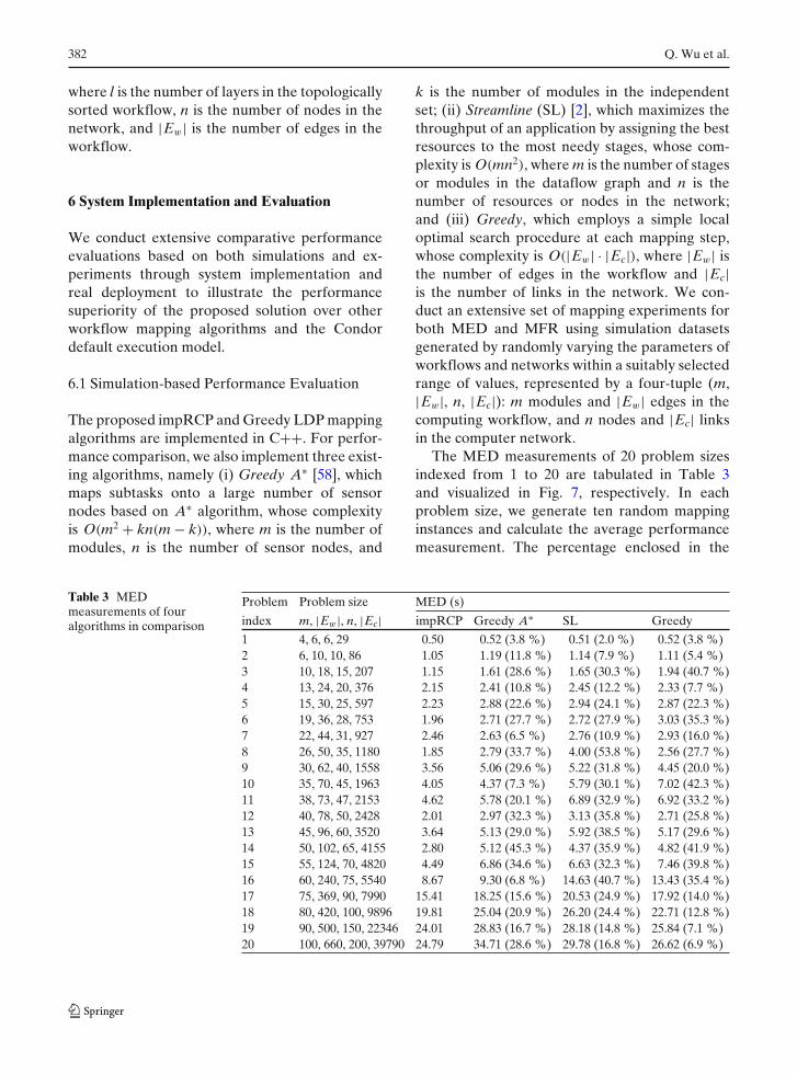
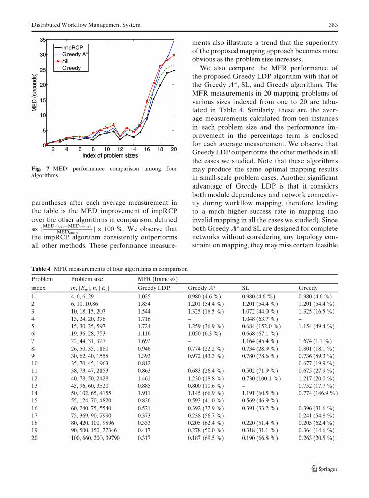
The MED measurements of 20 problem sizesindexed from 1 to 20 are tabulated in Table 3and visualized in Fig. 7, respectively. In eachproblem size, we generate ten random mappinginstances and calculate the average performancemeasurement. The percentage enclosed in the
Table 3 MEDmeasurements of fouralgorithms in comparison
Fig. 7 MED performance comparison among fouralgorithms
parentheses after each average measurement inthe table is the MED improvement of impRCPover the other algorithms in comparison, definedas |MEDothers−MEDimpRCP
MEDothers| × 100 %. We observe that
the impRCP algorithm consistently outperformsall other methods. These performance measure-
ments also illustrate a trend that the superiorityof the proposed mapping approach becomes moreobvious as the problem size increases.
We also compare the MFR performance ofthe proposed Greedy LDP algorithm with that ofthe Greedy A∗, SL, and Greedy algorithms. TheMFR measurements in 20 mapping problems ofvarious sizes indexed from one to 20 are tabu-lated in Table 4. Similarly, these are the aver-age measurements calculated from ten instancesin each problem size and the performance im-provement in the percentage term is enclosedfor each average measurement. We observe thatGreedy LDP outperforms the other methods in allthe cases we studied. Note that these algorithmsmay produce the same optimal mapping resultsin small-scale problem cases. Another significantadvantage of Greedy LDP is that it considersboth module dependency and network connectiv-ity during workflow mapping, therefore leadingto a much higher success rate in mapping (noinvalid mapping in all the cases we studied). Sinceboth Greedy A∗ and SL are designed for completenetworks without considering any topology con-straint on mapping, they may miss certain feasible
Table 4 MFR measurements of four algorithms in comparison
Problem Problem size MFR (frames/s)
index m, |Ew|, n, |Ec| Greedy LDP Greedy A∗ SL Greedy
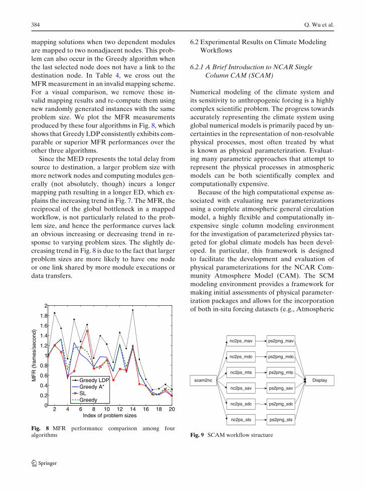
mapping solutions when two dependent modulesare mapped to two nonadjacent nodes. This prob-lem can also occur in the Greedy algorithm whenthe last selected node does not have a link to thedestination node. In Table 4, we cross out theMFR measurement in an invalid mapping scheme.For a visual comparison, we remove those in-valid mapping results and re-compute them usingnew randomly generated instances with the sameproblem size. We plot the MFR measurementsproduced by these four algorithms in Fig. 8, whichshows that Greedy LDP consistently exhibits com-parable or superior MFR performances over theother three algorithms.
Since the MED represents the total delay fromsource to destination, a larger problem size withmore network nodes and computing modules gen-erally (not absolutely, though) incurs a longermapping path resulting in a longer ED, which ex-plains the increasing trend in Fig. 7. The MFR, thereciprocal of the global bottleneck in a mappedworkflow, is not particularly related to the prob-lem size, and hence the performance curves lackan obvious increasing or decreasing trend in re-sponse to varying problem sizes. The slightly de-creasing trend in Fig. 8 is due to the fact that largerproblem sizes are more likely to have one nodeor one link shared by more module executions ordata transfers.
2 4 6 8 10 12 14 16 18 200
0.2
0.4
0.6
0.8
1
1.2
1.4
1.6
1.8
2
Index of problem sizes
MF
R (
fram
es/s
econ
d)
Greedy LDPGreedy A*SLGreedy
Fig. 8 MFR performance comparison among fouralgorithms
6.2 Experimental Results on Climate ModelingWorkflows
6.2.1 A Brief Introduction to NCAR SingleColumn CAM (SCAM)
Numerical modeling of the climate system andits sensitivity to anthropogenic forcing is a highlycomplex scientific problem. The progress towardsaccurately representing the climate system usingglobal numerical models is primarily paced by un-certainties in the representation of non-resolvablephysical processes, most often treated by whatis known as physical parameterization. Evaluat-ing many parametric approaches that attempt torepresent the physical processes in atmosphericmodels can be both scientifically complex andcomputationally expensive.
Because of the high computational expense as-sociated with evaluating new parameterizationsusing a complete atmospheric general circulationmodel, a highly flexible and computationally in-expensive single column modeling environmentfor the investigation of parameterized physics tar-geted for global climate models has been devel-oped. In particular, this framework is designedto facilitate the development and evaluation ofphysical parameterizations for the NCAR Com-munity Atmosphere Model (CAM). The SCMmodeling environment provides a framework formaking initial assessments of physical parameter-ization packages and allows for the incorporationof both in-situ forcing datasets (e.g., Atmospheric
scam2nc
nc2ps_mav
nc2ps_mdc
nc2ps_mts
nc2ps_sav
nc2ps_sdc
nc2ps_sts
ps2png_mav
ps2png_mdc
ps2png_mts
ps2png_sav
ps2png_sdc
ps2png_sts
Display
Fig. 9 SCAM workflow structure
Distributed Workflow Management System 385
scam2nc
nc2ps_mav
nc2ps_sts
ps2png_mav
ps2png_sts
Display
ps2png_sts_remove
nc2ps_mav_remove
nc2ps_sts_remove
ps2png_mav_remove
scam2nc_data
scam2nc_app
scam2nc_submit
scam2nc_remove
nc2ps_mav_data
nc2ps_mav_app
nc2ps_sts_data
nc2ps_sts_app
nc2ps_mav_submit
nc2ps_sts_submit
ps2png_mav_app
ps2png_sts_app
ps2png_sts_submit
ps2png_mav_submit
Fig. 10 SCAM executable workflow structure
Radiation Measurement (ARM) data) and syn-thetic, user-specified, and forcing datasets, to helpguide the refinement of parameterizations underdevelopment. Diagnostic data that are used toevaluate model performance can also be triviallyincorporated. The computational design of theSCM framework allows assessments of both thescientific and computational aspects of the physics
parameterizations for the NCAR CAM becausethe coding structures at the physics module lev-els are identical. This framework has widespreadutilities and helps enrich the pool of researchersworking on the problem of physical parameteriza-tion since few have access to or can afford testingnew approaches in atmospheric GCMs. Anotherstrength of this approach is that it provides a
Fig. 11 SCAM workflow generation
386 Q. Wu et al.
common framework to investigate the scientificrequirements for successful parameterization ofsubgrid-scale processes.
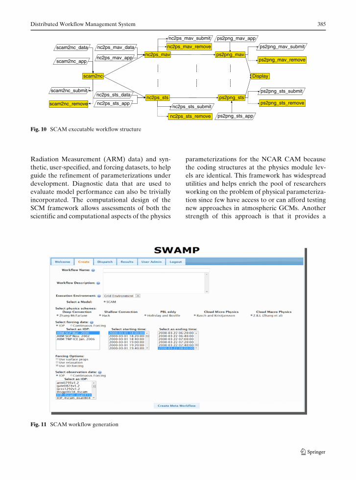
6.2.2 SCAM Workf low Structure
As shown in Fig. 9, we represent SCAM as aworkflow with 14 modules to be executed usingSWAMP in Grid environments with GridFTP-enabled inter-module data transfer. For each com-bination of available physics packages, data to beused, and experiment controls, we treat it as aseparate dispatch of one SCAM workflow. Thereare a dynamic number of workflow dispatchesfor the SCAM experiment depending on differentcombinations.
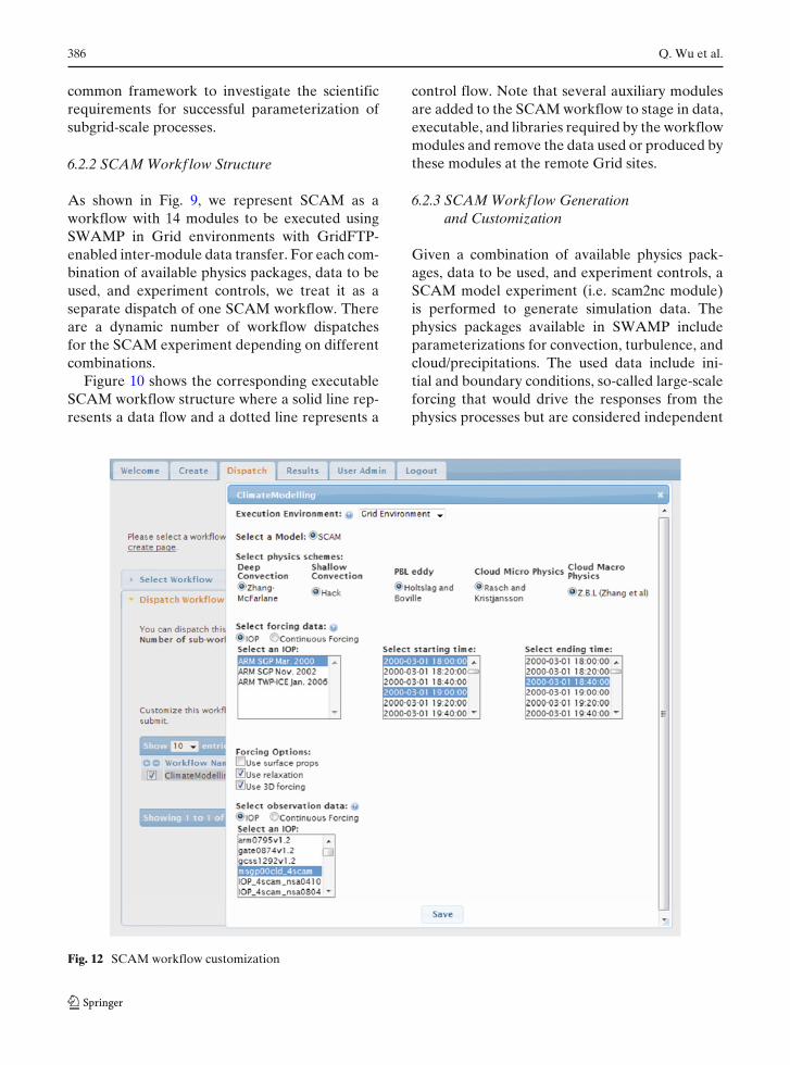
Figure 10 shows the corresponding executableSCAM workflow structure where a solid line rep-resents a data flow and a dotted line represents a
control flow. Note that several auxiliary modulesare added to the SCAM workflow to stage in data,executable, and libraries required by the workflowmodules and remove the data used or produced bythese modules at the remote Grid sites.
6.2.3 SCAM Workf low Generationand Customization
Given a combination of available physics pack-ages, data to be used, and experiment controls, aSCAM model experiment (i.e. scam2nc module)is performed to generate simulation data. Thephysics packages available in SWAMP includeparameterizations for convection, turbulence, andcloud/precipitations. The used data include ini-tial and boundary conditions, so-called large-scaleforcing that would drive the responses from thephysics processes but are considered independent
Fig. 12 SCAM workflow customization
Distributed Workflow Management System 387
. . . Display
nc2ps_mav ps2png_mav
nc2ps_mdc ps2png_mdc
nc2ps_sdc ps2png_sdc
nc2ps_sts ps2png_sts
. . . Display
nc2ps_mav ps2png_mav
nc2ps_mdc ps2png_mdc
nc2ps_sdc ps2png_sdc
nc2ps_sts ps2png_sts
. . . Display
nc2ps_mav ps2png_mav
nc2ps_mdc ps2png_mdc
nc2ps_sdc ps2png_sdc
nc2ps_sts ps2png_sts
100
stre
amin
g da
tase
ts in
tota
l
Control flow
Data flow
. . .
Wor
kflo
w 0
(0th
data
set)
scam2nc
Wor
kflo
w 1
(1th
data
set)
Wor
kflo
w 9
9(9
9th da
tase
t)
scam2nc
scam2nc
. . .
virtual module
virtual module
virtual module
. . .virtual module
virtual module
virtual module
. . .
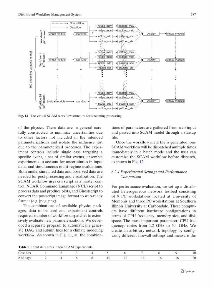
Fig. 13 The virtual SCAM workflow structure for streaming processing
of the physics. These data are in general care-fully constructed to minimize uncertainties dueto other factors not included in the intendedparameterizations and isolate the influence justdue to the parameterized processes. The exper-iment controls include single case targeting aspecific event, a set of similar events, ensembleexperiments to account for uncertainties in inputdata, and simultaneous multi-regime evaluations.Both model simulated data and observed data areneeded for post-processing and visualization. TheSCAM workflow uses csh script as a master con-trol, NCAR Command Language (NCL) script toprocess data and produce plots, and Ghostscript toconvert the postscript image format to web-readyformat (e.g. jpeg, png).
The combinations of available physics pack-ages, data to be used and experiment controlsrequire a number of workflow dispatches to exten-sively evaluate new parameterizations. We devel-oped a separate program to automatically gener-ate DAG and submit files for a climate modelingworkflow. As shown in Fig. 11, all the combina-
tions of parameters are gathered from web inputand passed into SCAM model through a startupfile.
Once the workflow meta file is generated, oneSCAM workflow will be dispatched multiple timesimmediately in a batch mode and the user cancustomize the SCAM workflow before dispatch,as shown in Fig. 12.
6.2.4 Experimental Settings and PerformanceComparison
For performance evaluation, we set up a distrib-uted heterogeneous network testbed consistingof 9 PC workstations located at University ofMemphis and three PC workstations at SouthernIllinois University at Carbondale. These comput-ers have different hardware configurations interms of CPU frequency, memory size, and diskspace. The most important parameter, CPU fre-quency, varies from 1.2 GHz to 3.4 GHz. Wecreate an arbitrary network topology by config-uring different firewall settings and measure the
Table 5 Input data sizes in ten SCAM experiments
Case Idx 1 2 3 4 5 6 7 8 9 10
# of days 2 4 6 8 10 12 14 16 18 20
388 Q. Wu et al.
1 2 3 4 5 6 7 8 9 1012
24
36
48
60
72
Index of problem cases
MF
R (
fram
es/m
inut
e)
Greedy LDPRandomRound RobinGreedy A*
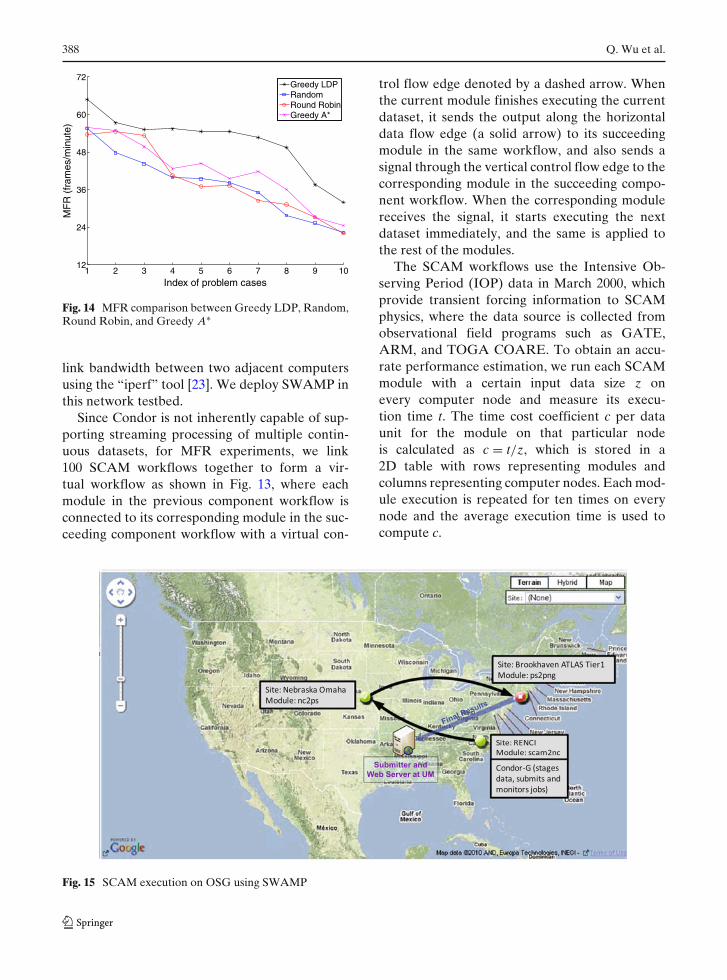
Fig. 14 MFR comparison between Greedy LDP, Random,Round Robin, and Greedy A∗
link bandwidth between two adjacent computersusing the “iperf” tool [23]. We deploy SWAMP inthis network testbed.
Since Condor is not inherently capable of sup-porting streaming processing of multiple contin-uous datasets, for MFR experiments, we link100 SCAM workflows together to form a vir-tual workflow as shown in Fig. 13, where eachmodule in the previous component workflow isconnected to its corresponding module in the suc-ceeding component workflow with a virtual con-
trol flow edge denoted by a dashed arrow. Whenthe current module finishes executing the currentdataset, it sends the output along the horizontaldata flow edge (a solid arrow) to its succeedingmodule in the same workflow, and also sends asignal through the vertical control flow edge to thecorresponding module in the succeeding compo-nent workflow. When the corresponding modulereceives the signal, it starts executing the nextdataset immediately, and the same is applied tothe rest of the modules.
The SCAM workflows use the Intensive Ob-serving Period (IOP) data in March 2000, whichprovide transient forcing information to SCAMphysics, where the data source is collected fromobservational field programs such as GATE,ARM, and TOGA COARE. To obtain an accu-rate performance estimation, we run each SCAMmodule with a certain input data size z onevery computer node and measure its execu-tion time t. The time cost coefficient c per dataunit for the module on that particular nodeis calculated as c = t/z, which is stored in a2D table with rows representing modules andcolumns representing computer nodes. Each mod-ule execution is repeated for ten times on everynode and the average execution time is used tocompute c.
Fig. 15 SCAM execution on OSG using SWAMP
Distributed Workflow Management System 389
Since there are 20 days of IOP data availablein March 2000, we choose a different number ofdays in each experiment to control the input datasize. Table 5 lists the number of days used in tenSCAM workflow experiments.
We run SCAM streaming experiments usingthe data sizes in Table 5 to compare the MFRmeasurements of the proposed Greedy LDP algo-rithm with those of the Random, Round Robin,and Greedy A∗ workflow mapping algorithms.The Random algorithm assigns each SCAM mod-ule to one of the 12 computers on a randombasis while the Round Robin algorithm assignsSCAM modules to the 12 computers in a round-robin manner. The performance curves producedby these four algorithms are plotted in Fig. 14. Weobserve that Greedy LDP outperforms the otherthree algorithms in all the cases we studied. Sincewe use the same workflow structure and mappingscheme for different input data sizes (which is
different from the simulation setting), a largerdata size is more likely to have a longer executiontime, resulting in a smaller MFR, which explainsthe decreasing trend in each curve. We do nothave the performance comparison in the OSGenvironment because the resource information re-quired by the mapping schemes are not availableon OSG, which does not provide detailed node in-formation within each Grid site but only the high-level site information via information services.
6.3 A Real-life Use Case: Climate ModelingWorkflow on Open Science Grid (OSG)
6.3.1 SCAM Workf low Execution on OSG
SWAMP provides a web-based interface to au-tomate and manage the SCAM workflow ex-ecution and uses a special site-level workflow
Fig. 16 A gallery of final images generated by the SCAM workflow executed on OSG using SWAMP
390 Q. Wu et al.
mapper to optimize its end-to-end performanceon OSG.
Figure 15 shows an example mapping of theSCAM workflow onto three OSG sites. In thisexample, DAGMan Manager and Condor-G areinstalled on the submit machine belonging to en-gagement virtual organization at University ofNorth Carolina. Condor-G stages in the executa-bles, libraries and data of all the modules tothe corresponding Grid sites in parallel usingGridFTP and submits the first scam2nc moduleto RENCI site at University of North Carolina.After the scam2nc module completes, Condor-Gstages out its output to the Nebraska Omaha siteat University of Nebraska using GridFTP andsubmits all the nc2ps modules to this site. Atthe same time when all the nc2ps modules arerunning on the Nebraska Omaha site, SWAMPruns scam2nc_submit and scam2nc_remove jobsto transfer the output of scam2nc back to thesubmit machine in order to keep track of thedata provenance and remove all the data usedor produced by scam2nc. When any of the nc2psmodules finishes execution, Condor-G stages outits output to the Brookhaven Atlas Tier1 siteat Brookhaven National Laboratory (BNL) andsubmits the corresponding ps2png module to thissite. At the same time when the ps2png mod-ules are running on the Brookhaven Atlas Tier1site, the SWAMP system runs correspondingnc2ps_submit and nc2ps_remove jobs to transferthe output of nc2ps modules back to the sub-mit machine in order to keep track of the dataprovenance and remove all the data used or pro-duced by nc2ps modules. Condor-G stages out thedata from BNL to the Web Server at Universityof Memphis using GridFTP for display and alsosends those png files back to the submit machinefor data provenance.
6.3.2 Display of SCAM Workf low Results
Each SCAM workflow eventually generates anumber of images. A gallery of final imagesfor one SCAM workflow are provided on theweb interface for a visual examination, as shownin Fig. 16. Also, based on the displayed re-sults, SWAMP enables the user to customize
those steerable computing modules of the SCAMworkflow and re-dispatch them into the Grid.
7 Conclusion
We developed a scientific workflow system basedon web services, SWAMP, for application usersto conveniently assemble, execute, monitor, andcontrol complex computing workflows in hetero-geneous network environments. We proposed twoefficient mapping algorithms, impRCP for MEDand Greedy LDP for MFR, and incorporatedthem into SWAMP for performance optimiza-tion. The system was implemented, deployed, andtested for a real-life scientific application in OpenScience Grid.
We learned a valuable lesson in the real sys-tem implementation that the workflow perfor-mance highly relies on the quality of the mappingscheme, which in turn relies on the accuracy of theperformance modeling and estimation. The time-varying nature of system and network resources’availability makes it very challenging to performan accurate estimation of the execution time ofa module or the transfer time over a link in realnetworks. We will investigate sophisticated costmodels to characterize real-time node and link be-haviors in dynamic network environments. Also,the overhead brought by Stork may counteractthe performance improvement of distributed ex-ecution in small problem sizes, but it is worth theeffort for workflows with large data sizes, whichare common in large-scale scientific applications.
Acknowledgements This research is sponsored by U.S.Department of Energy’s Office of Science under GrantNo. DE-SC0002400 with University of Memphis and GrantNo. DE-SC0002078 with Southern Illinois University atCarbondale. Lin and Liu are supported by the DOEEarth System Modeling (ESM) Program via the FASTERproject. We would like to thank two anonymous reviewersfor their insightful and constructive comments.
References
1. Afrati, F., Papadimitriou, C., Papageorgiou, G.:Scheduling DAGs to minimize time and communi-cation. In: Proc. of the 3rd Aegean Workshop on
Distributed Workflow Management System 391
Computing: VLSI Algorithms and Architectures,pp. 134–138. Springer, Berlin (1988)
2. Agarwalla, B., Ahmed, N., Hilley, D., Ramachandran,U.: Streamline: a scheduling heuristic for streaming ap-plication on the Grid. In: Proc. of the 13th MultimediaComp. and Net. Conf. San Jose, CA (2006)
3. Ahmed, I., Kwok, Y.: On exploiting task duplicationin parallel program scheduling. IEEE Trans. ParallelDistrib. Syst. 9, 872–892 (1998)
5. Bandwidth Test Controller: http://www.internet2.edu/performance/bwctl/. Accessed 1 Aug 2012
6. Boeres, C., Filho, J., Rebello, V.: A cluster-based strat-egy for scheduling task on heterogeneous processors.In: Proc. of 16th Symp. on Comp. Arch. and HPC,pp. 214–221 (2004)
7. Bozdag, D., Catalyurek, U., Ozguner, F.: A task dupli-cation based bottom-up scheduling algorithm for het-erogeneous environments. In: Proc. of the 20th IPDPS(2006)
9. Churches, D., Gombas, G., Harrison, A., Maassen, J.,Robinson, C., Shields, M., Taylor, I., Wang, I.: Prog-ramming scientific and distributed workflow with trianaservices. Concurrency and Computation: Practice andExperience, Special Issue: Workflow in Grid Systems18(10), 1021–1037 (2006). http://www.trianacode.org
10. Climate and Carbon Research Institute: http://www.ccs.ornl.gov/CCR. Accessed 1 Aug 2012
11. Cordella, L., Foggia, P., Sansone, C., Vento, M.: An im-proved algorithm for matching large graphs. In: Proc.of the 3rd Int. Workshop on Graph-based Representa-tions, Italy (2001)
12. DAGMan: http://www.cs.wisc.edu/condor/dagman.Accessed 1 Aug 2012
13. Dean, J., Ghemawat, S.: MapReduce: simplified dataprocessing on large clusters. In: Proc. of 6th Symp.on Operating System Design and Implementation, SanFrancisco, CA (2004)
14. Deelman, E., Gannon, D., Shields, M., Taylor, I.:Workflows and e-Science: an overview of workflowsystem features and capabilities. J. of Future Genera-tion Comp. Sys. 25(5), 528–540 (2009)
15. Deelman, E., Singh, G., Su, M., Blythe, J., Gil, A.,Kesselman, C., Mehta, G., Vahi, K., Berriman, G.B.,Good, J., Laity, A., Jacob, J.C., Katz, D.S.: Pegasus: aframework for mapping complex scientific workflowsonto distributed systems. Sci. Program. 13, 219–237(2005)
16. Dhodhi, M., Ahmad, I., Yatama, A.: An integratedtechnique for task matching and scheduling onto dis-tributed heterogeneous computing systems. JPDC 62,1338–1361 (2002)
17. Distributed computing projects: http://en.wikipedia.org/wiki/List_of_distributed_computing_projects. Ac-cessed 1 Aug 2012
18. Dobber, M., van der Mei, R., Koole, G.: A predictionmethod for job runtimes on shared processors: survey,statistical analysis and new avenues. Perform. Eval.64(7–8), 755–781 (2007)
19. Earth Simulator Center: http://www.jamstec.go.jp/esc.Accessed 1 Aug 2012
20. Earth System Grid (ESG): http://www.earthsystemgrid.org. Accessed 1 Aug 2012
21. Fahringer, T., Prodan, R., Duan, R., Nerieri, F.,Podlipnig, S., Qin, J., Siddiqui, M., Truong, H.-L., Vil-lazon, A., Wieczorek, M.: ASKALON: a Grid appli-cation development and computing environment. In:Proc. of the 6th IEEE/ACM Int. Workshop on GridComp., pp. 122–131 (2005)
22. Garey, M., Johnson, D.: Computers and Intractability:A Guide to the Theory of NP-completeness. Freeman,San Francisco (1979)
23. Gates, M., Warshavsky, A.: Iperf version 2.0.3.http://iperf.sourceforge.net. Accessed 1 Aug 2012
24. Gerasoulis, A., Yang, T.: A comparison of clusteringheuristics for scheduling DAGs on multiprocessors.JPDC 16(4), 276–291 (1992)
25. Globus Replica Location Service: http://www.globus.org/toolkit/data/rls/. Accessed 1 Aug 2012
26. GridFTP: http://www.globus.org/grid_software/data/gridftp.php. Accessed 1 Aug 2012
27. Gu, Y., Wu, Q.: Maximizing workflow throughput forstreaming applications in distributed environments. In:Proc. of the 19th Int. Conf. on Comp. Comm. and Net.,Zurich, Switzerland (2010)
28. Gu, Y., Wu, Q.: Optimizing distributed computingworkflows in heterogeneous network environments.In: Proc. of the 11th Int. Conf. on DistributedComputing and Networking, Kolkata, India, 3–6 Jan2010
29. Gu, Y., Wu, Q., Benoit, A., Robert, Y.: Optimiz-ing end-to-end performance of distributed applicationswith linear computing pipelines. In: Proc. of the 15thInt. Conf. on Para. and Dist. Sys., Shenzhen, China, 8–11 Dec 2009
30. Hull, D., Wolstencroft, K., Stevens, R., Goble, C.,Pocock, M., Li, P., Oinn, T.: Taverna: a tool for buildingand running workflows of services. Nucleic Acids Res34, 729–732 (2006). http://www.taverna.org.uk
31. Ilavarasan, E., Thambidurai, P.: Low complexity per-formance effective task scheduling algorithm for het-erogeneous computing environments. J. Comp. Sci.3(2), 94–103 (2007)
32. Johnston, W.: Computational and data Grids in large-scale science and engineering. J. of Future GenerationComp. Sys. 18(8), 1085–1100 (2002)
33. Kacsuk, P., Farkas, Z., Sipos, G., Toth, A., Hermann,G.: Workflow-level parameter study management inmulti-Grid environments by the P-GRADE Grid por-tal. In: Int. Workshop on Grid Computing Enviorn-ments (2006)
38. Lewis, T., EI-Rewini, H.: Introduction to Parallel Com-puting. Prentice Hall, New York (1992)
39. Load Sharing Facility: http://www.platform.com/workload-management/high-performance-computing/lp.Accessed 1 Aug 2012
40. Ludäscher, B., Altintas, I., Berkley, C., Higgins, D.,Jaeger-Frank, E., Jones, M., Lee, E., Tao, J., Zhao,Y.: Scientific workflow management and the Keplersystem. Concurrency and Computation: Practice andExperience 18(10), 1039–1605 (2006)
41. Ma, T., Buyya, R.: Critical-path and priority basedalgorithms for scheduling workflows with parametersweep tasks on global Grids. In: Proc. of the 17th Int.Symp. on Computer Architecture on HPC, pp. 251–258(2005)
42. McCreary, C., Khan, A., Thompson, J., McArdle, M.:A comparison of heuristics for scheduling DAGs onmultiprocessors. In: Proc. of the 8th ISPP, pp. 446–451(1994)
43. McDermott, W., Maluf, D., Gawdiak, Y., Tran,P.: Airport simulations using distributed computa-tional resources. J. Defense Soft. Eng. 16(6), 7–11(2003)
44. Messmer, B.: Efficient graph matching algorithms forpreprocessed model graphs. PhD thesis, Institute ofComputer Science and Applied Mathematics, Univer-sity of Bern (1996)
45. Monitoring and Discovery System (MDS): http://www.globus.org/toolkit/mds/. Accessed 1 Aug 2012
46. Network weather service: http://nws.cs.ucsb.edu.Accessed 1 Aug 2012
47. One-Way Active Measurement Protocol: http://www.internet2.edu/performance/owamp/. Accessed 1 Aug2012
48. Open Science Grid: http://www.opensciencegrid.org.Accessed 1 Aug 2012
49. OSCARS: On-demand Secure Circuits and Ad-vance Reservation System: http://www.es.net/oscars.Accessed 1 Aug 2012
50. OSG Resource and Site Validation: http://vdt.cs.wisc.edu/components/osg-rsv.html. Accessed 1 Aug 2012
51. Performance Inspector: http://perfinsp.sourceforge.net.Accessed 1 Aug 2012
53. Portable Batch System: http://www.pbsworks.com/.Accessed 1 Aug 2012
54. Rahman, M., Venugopal, S., Buyya, R.: A dynamic crit-ical path algorithm for scheduling scientific workflowapplications on global Grids. In: Proc. of the 3rdIEEE Int. Conf. on e-Sci. and Grid Comp., pp. 35–42(2007)
55. Ranaweera, A., Agrawal, D.: A task duplication basedalgorithm for heterogeneous systems. In: Proc. ofIPDPS, pp. 445–450 (2000)
56. Rao, N.S.V.: Vector space methods for sensor fusionproblems. Opt. Eng. 37(2), 499–504 (1998)
57. Reliable File Transfer: http://www-unix.globus.org/toolkit/docs/3.2/rft/index.html. Accessed 1 Aug 2012
58. Sekhar, A., Manoj, B., Murthy, C.: A state-space searchapproach for optimizing reliability and cost of execu-tion in distributed sensor networks. In: Proc. of Int.Workshop on Dist. Comp., pp. 63–74 (2005)
59. Shroff, P., Watson, D., Flann, N., Freund, R.: Geneticsimulated annealing for scheduling data-dependenttasks in heterogeneous environments. In: Proc. ofHeter. Comp. Workshop, pp. 98–104 (1996)
60. Singh, M., Vouk, M.: Scientific workflows: scientificcomputing meets transactional workflows. In: Proc. ofthe NSF Workshop on Workflow and Process Automa-tion in Information Systems: State-of-the-Art and Fu-ture Directions, pp. 28–34. Univ. Georgia, Athens, GA(1996)
61. Spallation Neutron Source: http://neutrons.ornl.gov,http://www.sns.gov. Accessed 1 Aug 2012
62. Storage Resource Broker (SRB): http://www.sdsc.edu/srb/index.php/Main_Page. Accessed 1 Aug 2012
63. Storage Resource Management (SRM): https://sdm.lbl.gov/srm-wg/. Accessed 1 Aug 2012
64. Stork: http://www.cct.lsu.edu/∼kosar/stork/index.php.Accessed 1 Aug 2012
65. Swift: http://www.ci.uchicago.edu/swift/main/.Accessed 1 Aug 2012
66. Taylor, I.J., Deelman, E., Gannon, D.B., Shields, M.(eds.): Workflows for e-Science: Scientific Workflowsfor Grids. Springer, Berlin Heidelberg New York (2007)
67. TeraPaths: https://www.racf.bnl.gov/terapaths.Accessed 1 Aug 2012
68. The Whetstone Benchmark: http://www.roylongbottom.org.uk/whetstone.htm. Accessed 1 Aug 2012
69. Topcuoglu, H., Hariri, S., Wu, M.: Performanceeffective and low-complexity task scheduling for het-erogeneous computing. IEEE TPDS 13(3), 260–274(2002)
70. Wang, L., Siege, H., Roychowdhury, V., Maciejewski,A.: Task matching and scheduling in heterogeneouscomputing environments using a genetic-algorithm-based approach. JPDC 47, 8–22 (1997)
71. Wassermann, B., Emmerich, W., Butchart, B.,Cameron, N., Chen, L., Patel, J.: Workflows fore-Science: Scientific Workflows for Grids, ChapterSedna: A BPEL-based Environment for VisualScientific Workflow Modeling, pp. 427–448. Springer,London (2007)
72. Worldwide LHC Computing Grid (WLCG):http://lcg.web.cern.ch/LCG. Accessed 1 Aug 2012
73. Wu, Q., Gu, Y.: Optimizing end-to-end performanceof data-intensive computing pipelines in heterogeneousnetwork environments. J. Parallel Distrib. Comput.71(2), 254–265 (2011)
74. Wu, Q., Gu, Y., Liao, Y., Lu, X., Lin, Y., Rao, N.:Latency modeling and minimization for large-scale
scientific workflows in distributed network envi-ronments. In: The 44th Annual Simulation Sym-posium (ANSS11), Part of the 2011 Spring Simu-lation Multiconference (SpringSim11), Boston, MA,4–7 Apr 2011
75. Wu, Q., Rao, N.S.V.: On transport daemons for smallcollaborative applications over wide-area networks. In:Proc. of the 24th IEEE Int. Performance Computing
and Communications Conf., pp. 159–166, Phoenix, AZ,7–9 Apr 2005
76. Wu, Q., Zhu, M., Lu, X., Brown, P., Lin, Y., Gu,Y., Cao, F., Reuter, M.: Automation and manage-ment of scientific workflows in distributed networkenvironments. In: Proc. of the 6th Int. Workshopon Sys. Man. Tech., Proc., and Serv., Atlanta, GA,19 Apr 2010